Article

New Expressions to Apply the Variation Operation Strategy in Engineering Tools Using Pumps Working as Turbines

by
Frank A Plua
1,
Francisco-Javier Sánchez-Romero
2,
Victor Hidalgo
3,
P. Amparo López-Jiménez
4 and
Modesto Pérez-Sánchez
4,*
1
Civil and Environmental Engineering Department, Escuela Politécnica Nacional, Quito 170525, Ecuador
2
Rural and Agrifood Engineering Department, Universitat Politècnica de València, 46022 Valencia, Spain
3
Mechanical Engineering Department, Escuela Politécnica Nacional, Quito 170525, Ecuador
4
Hydraulic and Environmental Engineering Department, Universitat Politècnica de València, 46022 Valencia, Spain
*
Author to whom correspondence should be addressed.
Mathematics 2021, 9(8), 860; https://doi.org/10.3390/math9080860
Submission received: 26 February 2021 / Revised: 9 April 2021 / Accepted: 12 April 2021 / Published: 14 April 2021
(This article belongs to the Special Issue Applications of Mathematical Models in Engineering)

Abstract

:
The improvement in energy saving aspects in water systems is currently a topic of major interest. The utilization of pumps working as turbines is a relevant strategy in water distribution networks consisting of pressurized pipes, using these machines to recover energy, generate green energy and reduce leakages in water systems. The need to develop energy studies, prior to the installation of these facilities, requires the use of simulation tools. These tools should be able to define the operation curves of the machine as a function of the flow rate. This research proposes a new strategy to develop a mathematics model for pumps working as turbines (PATs), considering the modified affinity laws. This proposed model, which can be input into hydraulic simulation tools (e.g., Epanet, WaterGems), allows estimation of the head, efficiency, and power curves of the PATs when operating at different rotational speeds. The research used 87 different curves for 15 different machines to develop the new model. This model improves the results of the previously published models, reducing the error in the estimation of the height, efficiency, and power values. The proposed model reduced the errors by between 30 and 50% compared to the rest of the models.

1. Introduction

Mathematical models have been a very useful tool to improve the management of water networks [1]. These models improved both pressurized systems [2], as well as free surface channels [3], improving their management and behavior in steady and unsteady flows. Some of these models were focused on the integration of the management into the new sustainability challenges of the infrastructures [4].
The improvement of the sustainability has been analyzed in water systems from different points of view, such as leakage reduction [5], minimizing consumed energy in pump systems [6], and quality parameters in the water supply [7], among others. One of these strategies has been the use of pumps working as turbines (PATs). These machines replace the pressure reduction valves, taking advantage of the excess of energy in the pressurized water systems [8]. A PAT is a pump which works in reverse mode and it is cheaper than classical turbines of the same small size [9]. When this machine operates in this mode, it generates energy. The efficiency of these machines is lower than traditional turbines and its hydraulic efficiency value is between 0.6 and 0.7 [10]. The global efficiency is between 0.5 and 0.6 when all the electromechanical equipment (electric and electronic devices) is considered. The traditional machines are classified as action (e.g., Pelton, Turgo, among others) and reaction (Francis, Kaplan, among others), as described in [11]. In contrast, the PATs are pumps, and, therefore, their classification depends on the specific velocity (i.e., radial, mixed, or axial machines) [12,13].
Previously, different investigations were published in which the use and analysis of PATs focused on analyzing the theoretical energy recovery [11] as well as the duty point of these machines, when information about the manufacturer was not known [12]. When the curves are not known, the head, efficiency, and power curves (these curves are called characteristic curves of the PATs) should be estimated when the pump is used in turbine mode. These expressions are defined by the following equations:
H 0 = A + B Q 0 + C Q 0 2
η 0 = E 4 Q 0 4 + E 3 Q 0 3 + E 2 Q 0 2 + E 1 Q 0 + E 0
P 0 = P 4 Q 0 4 + P 3 Q 0 3 + P 2 Q 0 2 + P 1 Q 0 + P 5
where H 0 is the recovered head in nominal rotational speed in m w.c. (water column); Q 0 is the flow rate in m3/s; A ,   B ,   a n d   C are the coefficients, which define the head curve of the PAT; η 0 is the efficiency of the machine for each flow (non-dimensional); E 4 ,   E 3 ,   E 2 ,   E 1 ,   a n d   E 0 are the coefficients, which define the efficiency curve; P 0 is the generated power in kW; P 4 ,   P 3 ,   P 2 ,   P 1 ,   a n d   P 5 are the coefficients, defining the power curve of the machine.
The head curve enables the determination of the recovered head as a function of the flow. The efficiency curve determines the efficiency of the machine according to the circulating flow; finally, the power curve establishes the generated power by the machine for each flow value. Previous references demonstrated the possibility to estimate these curves by use of non-dimensional parameters [14]. This estimation should be developed using non-dimensional parameters and they are head number (h), flow number (q), efficiency number (e), and torque number (b) [15]. The different non-dimensional parameters, which are used to regulate the machines by variation of the rotational speed, are the following:
q = Q i Q B E P
h = H i H B E P
e = η i η B E P
p = P i P B E P = q h e
where q ,   h ,   e ,   a n d   p are the flow, head, efficiency, and power coefficients; Q i is any flow value of the PAT in m3/s; H i is the head for Q i according to the head curve in m w.c.; η i is the efficiency of the machine when the flow is Q i ; P i is the effective power for Q i ; Q B E P , H B E P , P B E P , and η B E P refer to the best efficiency point (BEP) of the machine, which define the best efficiency head (BEH) when the rotational speed is changed.
In line with this, the reduction of the uncertainties by estimating the characteristic curves with respect to their known behavior as pumps has been an objective of different studies [16]. Different semiempirical methods have been published, proposing polynomial expressions to estimate the PAT curves, when the machine operates with constant rotational speed [10,12,17,18]. The development of these mathematical expressions was crucial to improve the characterization of the PATs and the energy models to analyze the energy recovery.
However, the flow rate changes over time in the different pipes of the water networks due to the demands of the users. Therefore, the energy analyses are not maximized when they consider PATs, if they work under constant rotational speed. To increase energy recovery, different strategies have been published in which the energy maximization was reached when the machine operated at different rotational speeds, called the variable operation strategy (named VOS) [19]. The variation of the rotational speed is crucial to reach the best efficiency values in the water systems, and it is the focus of new challenges in hydropower systems also applied to Francis turbines [20]. Furthermore, when the rotation speed changes, it is necessary to introduce knowledge of PAT curves into mathematical models, which analyze energy recovery in water systems. The lack of mathematical expressions makes it difficult to improve energy estimates when applying the VOS strategy in the modeling of water systems [14].
In recent years, some researchers have published different methods which allow water managers and companies to estimate the characteristic curves of PATs, avoiding the experimental tests when developing preliminary energy studies. Efficiency and head curves operating without variation of rotational speed were described in [21,22]. The analysis of PAT curves was carried out using other methods, which proposed expressions considering specific speed as well as the best efficiency point [23,24,25]. These methods did not consider the variation in the rotational speed, which is of paramount importance to reach the maximization of the recovered energy [26].
A step forward was taken in 2014, when some researchers analyzed the variation in rotational speed through experimental tests to improve the maximization of energy recovery. Research described in [12] proposed empirical expressions using four different tested machines in 2016. These equations should only be considered when the specific speed is between 120 and 162 (m, kW). In 2018, two PATs were tested and they were used to define other expressions, which could estimate the characteristic curves when the best efficiency point was known [27]. Research published in [28] studied the efficiency, power, and head curves in one PAT, which was installed in water pressurized systems in 2020. All studies used between one and four machines [12,14,27,28]. The low number of machines reduces the applicability of the proposed expressions, when other machines are used. To solve this issue, the present research goes one step further, using 87 different tested characteristic curves (i.e., head, efficiency, and power) of the majority of hydraulic machines, which have been published in previous references.
New empirical expressions are here proposed. These expressions could be used by modelers, who could improve their energy analysis when they apply the VOS strategy in water systems. Previous research has conducted similar analyses to define the characteristic curves of the machine [12,14,27,28]. They used non-dimensional numbers (i.e., q, h, e, and p), which are calculated at the best efficiency point. These values were used to propose functions, which depended on the ratio of the rotational speed of the machine to modify the affinity laws. This proposal improves the use of PATs in the simulation tools. It will enable the reduction of the uncertainty in the previous energy analysis when the use of PATs is considered in a real case study. The proposed expressions reduced the error indexes when they were compared with the other published methods, as well as increasing the validity range. Furthermore, these expressions are based on fifteen different machines, which had 87 different curves, increasing the number of experimental curves.

2. Materials and Methods

2.1. Methodology

The methodology proposed herein is focused on obtaining some particular empiric expressions, which allow water managers to develop tools for modeling PATs in water systems, when they operate at variable rotational speed. The strategy is based on the knowledge of the operation curves (head, efficiency, and power) at nominal speed [29]. The proposed method is based on classical expressions of the hydraulic machines, proposing a strategy to modify them by the affinity laws.
The main objective of the strategy is to propose an empirical expression that allows water managers to introduce management tools to simulate the different scenarios under the VOS operation. Furthermore, the method will reduce the errors when the characteristic curves are estimated in variable velocity conditions. To achieve this, different steps were proposed to derive the new expressions considering the modification of the affinity laws of hydraulic machines. [30]. Finally, the method was validated with the different tested machines. Figure 1 shows the different proposed steps. These steps are the following:
  • Obtaining experimental characteristic curves of the PATs. The characteristic curves (i.e., head, efficiency, and power curve) were made available for the different machines using experimental data which were published by other researchers. Both the nominal curve and the curves for different rotational speeds were digitized using Equations (1)–(3).
  • Definition of the dimensionless values of the curve to apply the affinity laws. This is developed using the previously defined equations (Equations (4)–(8)). When the affinity laws are applied, the congruence parabola is defined by the following equation [29]:
    H P C = H 0 Q 0 2 Q j 2 = k A L Q j 2
    where Q j is the new flow rate in m3/s in which the machine has to operate. H P C is a parabola, which has the same efficiency at each point. This consideration is theoretical, since (in practice) it is only acceptable for values around +/−20% of the best efficiency point of the machine [29]. This variation in the rotational speed of the machine is defined by the ratio between the rotational speed ( n j ) of the machine to reach the value ( Q j ) and the nominal rotational speed ( n 0 ). This ratio between n j and n 0 is called α .
The affinity laws are expressions which define points similar to each other under conditions of restricted similarity, neglecting the stresses due to viscosity. These expression are defined by the following expressions [29]:
Q 1 Q 0 = n 1 n 0 = α
H 1 H 0 = ( n 1 n 0 ) 2 = α 2
P 1 P 0 = ( n 1 n 0 ) 3 = α 3
where Q 1 is the flow under the new conditions of rotational speed ( n 1 ) in m3/s; H 1 is the head under the new conditions in m w.c.; P 1 is the shaft power under the new conditions in kW.
When affinity laws are applied for different rotational speeds, the variable operation strategy (VOS) can be defined between ratios of α m i n and α m a x .
When affinity laws are applied, the dimensionless parameters are:
q = α
h = α 2
e = 1
p = α 3
Applying the affinity laws, k A L ,   B E H is defined by the following expression, considering that the ratio h q 2 = 1 (if the classical affinity laws is applied ideally):
k A L , B E H = A Q B E P 2 + B Q B E P + C
3.
Once the dimensionless parameters ( q ,   h ,   e ,   a n d   p ) are defined, the best efficiency curve (BEH) of the machine is determined. BEH is the curve which establishes the recovered head for each flow, maximizing efficiency and changing the rotation speed of the machine. This curve is defined in [27].
4.
When the BEH is known for each machine, the ratio h / q 2 is defined for the different values, using the experimental data as well as the regression of the different head and efficiency curves. This parameter is defined for each rotational speed of the machine. The rotational speed varies between the α m i n and α m a x of the VOS. The operation area is defined by the maximum and minimum rotational speed, determined by the tested machine.
5.
In [27,31], variations of the affinity laws are proposed, where the flow ratio ( Q / Q 0 ) is a function that depends on α ; taking into account this modification of the affinity laws, the corresponding parameter k A L for the modified affinity laws (MOAL) can be defined when the affinity laws are modified by the following expression:
k M O A L , B E H = h q 2 ( A Q B E P 2 + B Q B E P + C )
6.
The value of the k M O A L ,   B E H coefficient is defined for the different rotational speeds of the machine, determining the cut-off point with the hypothetical head surface and machine efficiency (Figure 2).
Once the k M O A L ,   B E H is defined using Q B E P and H B E P , k M O A L is extended for different values of Q 0 , defining the k M O A L , i for each rotational speed and the intersection points with head and efficiency areas are calculated. These points are Q 0 , H 0 , η 0 , Q i , α j , H i , α j and η i , α j (Figure 3a,b). The values of these parameters enable definition of the new non-dimensional values, which will define the functions of the modified affinity laws. Each of these points is calculated considering the intersection point for each rotational speed curve. The new non-dimensional parameters are defined by the following expressions:
q i , j = Q i , α j Q i , 0
h i , j = H i , α j H i , 0
η i , j = η i , α j η i , 0
7.
Once the non-dimensional parameters for the different rotational speeds are defined, the regression expressions are proposed. These functions depend on rotational speed ( α ), which is a significant variable [31] when the non-dimensional parameters are defined (i.e., h ,   q ,   a n d   e ). Moreover, different expressions are also proposed considering the ratio Q / Q B E P . This parameter is considered since it measures the gap between the flow value and the flow for the best efficiency point. The incorporation of this parameter will improve the regression coefficient of the expressions, as well as reducing the errors. The modified affinity laws are then defined according to different expressions:
H = h ( A + B Q q + C ( Q q ) 2 )
η = e   ( E 4 ( Q q ) 4 + E 3 ( Q q ) 3 + E 2 ( Q q ) 2 + E 1 ( Q q ) + E 0 )
P = p   ( P 4 ( Q q ) 4 + P 3 ( Q q ) 3 + P 2 ( Q q ) 2 + P 1 ( Q q ) + P 5 )
Ten different functions ( F i ) were proposed, in order to be analyzed and obtain the best one to estimate the behavior of the machine when it operates at variable rotational speed. Table 1 shows the proposed functions in which the different coefficients ( β i ) are calculated as a function on the analyzed F i . This analysis proposes six polynomial functions and four exponential expressions.
8.
This step is related to the previous step and concerns the recalculation of the coefficients β i considering the values of all the tested machines q i , j , m ,   h i , j , m ,   a n d   e i , j , m . The sub-index “m” refers to each tested machine.
9.
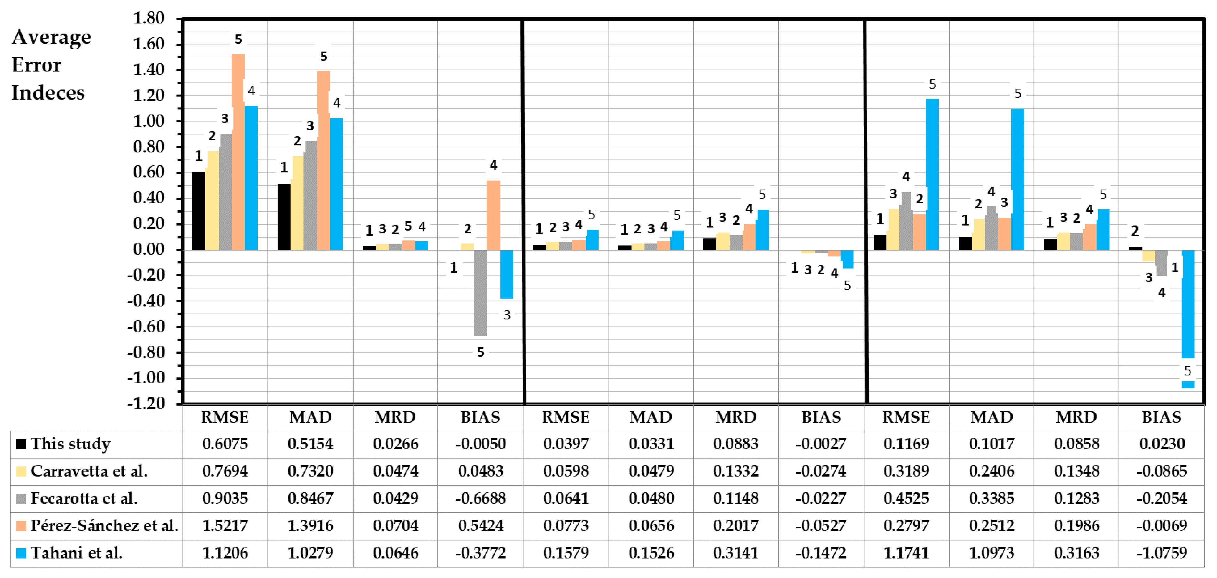
Having the coefficients for the different functions ( F i ) as well as the non-dimensional parameters ( i . e . ,   h ,   q ,   e , h q 2 , h e q 2 ) defined, the errors of the proposed functions by MOAL are calculated. The error indices considered were root mean square error (RMSE), mean absolute deviation (MAD), the mean relative deviation (MRD), and BIAS:
(a)
RMSE. This error index measures the error between the empirical expression and experimental values. When RMSE is zero, this value indicates a perfect fit. It is defined by (24):
R M S E = i = 1 x [ O i P i ] 2 x
where O i are the estimated values; P i the experimental values, and x is the number of observations.
(b)
MAD. This index measures the average of the errors in the estimated values, using the absolute differences between estimated and experimental values. The perfect fit is defined when MAD is zero, and it is defined by the following expression (25):
M A D = 1 x 1 x | O i P i |
(c)
MRD. This index considers the weight of the error to the variable value. If MRD is zero, this value indicates a perfect fit. Formally, it is defined as follows (26):
M R D = 1 x | O i P i | / P i x
(d)
BIAS. The index considers the variable tendency, analyzing whether the estimated values are greater (negative value) or smaller (positive value) than experimental values. It is defined by the following expression (27):
B I A S = i = 1 N [ O i P i ] x
If the error values are acceptable and the goodness of the expressions is correct, the best expression is chosen in order to be applied. The best expression should set low error values, and it should consider a smaller number of variables.

2.2. Materials

The proposed methodology was applied using different experimental machines. As indicated, 15 PATs were used in this research, as shown in Table 2. The experimental database was developed from different consulted studies. These PATs were tested considering different rotation speeds (Table 3), which allowed interpolation of the different experimental values among rotation speeds. The specific speed ( n s t ) of the used machines was between 5 and 50 rpm. n s t is defined as:
n s t = n 0 P 0 1 2 H 0 5 4
Table 2 also shows the number of experimental curves (RS) which were tested considering different rotational speeds for each machine, the number of interpolated curves used, as well as the number of used points to develop the regression and database analysis. The analysis of the 87 tested curves for different PATs, which operated on different rotational speeds, enabled us to obtain 10,949 interpolated parabolas, as well as 56,450 work points, to develop the surface (Q, H, α ; Figure 2).

3. Results

3.1. Proposed Function Models

Once the experimental data from the referred 15 tested PATs were analyzed, the β i coefficients were determined for the different non-dimensional parameters (i.e., q ,   h ,   e ,   p ,   h / q 2 ,   h e / q 2 ). Table 3 shows the different values of coefficients β i for each proposed function ( F i ) to model the non-dimensional parameters ( N P ). Table 3 also shows the regression coefficient (R2).
The goodness of these models was measured according to the different error indexes, which were described previously in the Methodology section by Equations (21)–(23). The different dimensionless parameters proposed for each machine and rotation speed were determined, defining the error rates for the ten different functions of the model. Table 4 shows the error values for each index, as well as its ranking compared among the ten functions. This table determines the average values of the error indexes, since these errors were calculated for each rotational speed in each tested machine (87 curves). BIAS shows the absolute value, in order to know the magnitude of this error in case of oversize or undersize of a variable (i.e., H ,   η ,   a n d   P ).
Table 4 shows the average error values for each FM. These errors values enable us to decide the best function model for each dimensionless parameter (i.e., h, q, e, and p). When the error analysis was developed, the best function model (FM) was F6 for h and e dimensionless parameters. Although different FMs could be used, F6 considered both rotational speed as well as the ratio Q Q B E P . The use of this ratio is interesting since it measures the distance between Q and Q B E P . This is an important difference, since it allows water managers to fix the operation range of flow in order for the affinity laws to be applied [29].
When non-parameter p was analyzed, the F7 function also was chosen since it only considered one variable ( α ), yielding good results in the estimation of the PATs curve. F7 was used to determine the power curve directly by expression (23). However, when water managers wish to determine the power curve by the use of Q, H, and η , they should use the F6 function.

3.2. Error Distribution Compared to Rotational Speed

Once F6 was chosen, the error of the modified affinity laws was compared with all tested curves. All error indexes were calculated for head, efficiency, and power.
When head was analyzed, the MRD was smaller than 0.05, with a cumulated frequency equal to 91%. The maximum value was 0.089. In head values, RMSE was smaller than 0.6 in 57 compared curves and BIAS was smaller than 0.25 in 49 compared curves.
When efficiency was compared, RMSE was smaller than 0.035 in 58% of the comparisons and it was smaller than 0.07 in 88% of the comparisons. When MRD was checked, it was smaller than 0.15, showing a BIAS value smaller than 0.069 in 92% of the cases.
When the error values for the power curve using the F6 function model were analyzed, RMSE was smaller than 0.2 (72% cumulated frequency). When MAD was analyzed, similar values were obtained. MAD was lower than 0.17, and the MRD was smaller than 0.2 in 90% of the samples.
However, when the errors of F7 were analyzed for the power curve, they showed the best approach. Figure 4 shows the error values for the power curve using the F7 expression. RMSE was analyzed (Figure 4a), and it was smaller than 0.18 (70% of cumulated frequency). This value was smaller than 0.09 in 51 cases. Moreover, when the α value was observed, smaller values were located between 0.8 and 1.2, reaching a minimum around 0.9.
When MAD was analyzed (Figure 4b), similar values were obtained. In this case, MAD values were smaller than 0.16 (92% of cumulated frequency). When MRD was analyzed (Figure 4c), this value was smaller than 0.2 in 94% of the samples. This value had a value of 65% of cumulated frequency for values lower than 0.07. Finally, BIAS had good accuracy, showing values lower than 0.1 in 85% of the sample. In all cases, the minimum errors were reached when the machine operated using α rates between 0.8 and 1.2, being the minimum for values near 0.9.

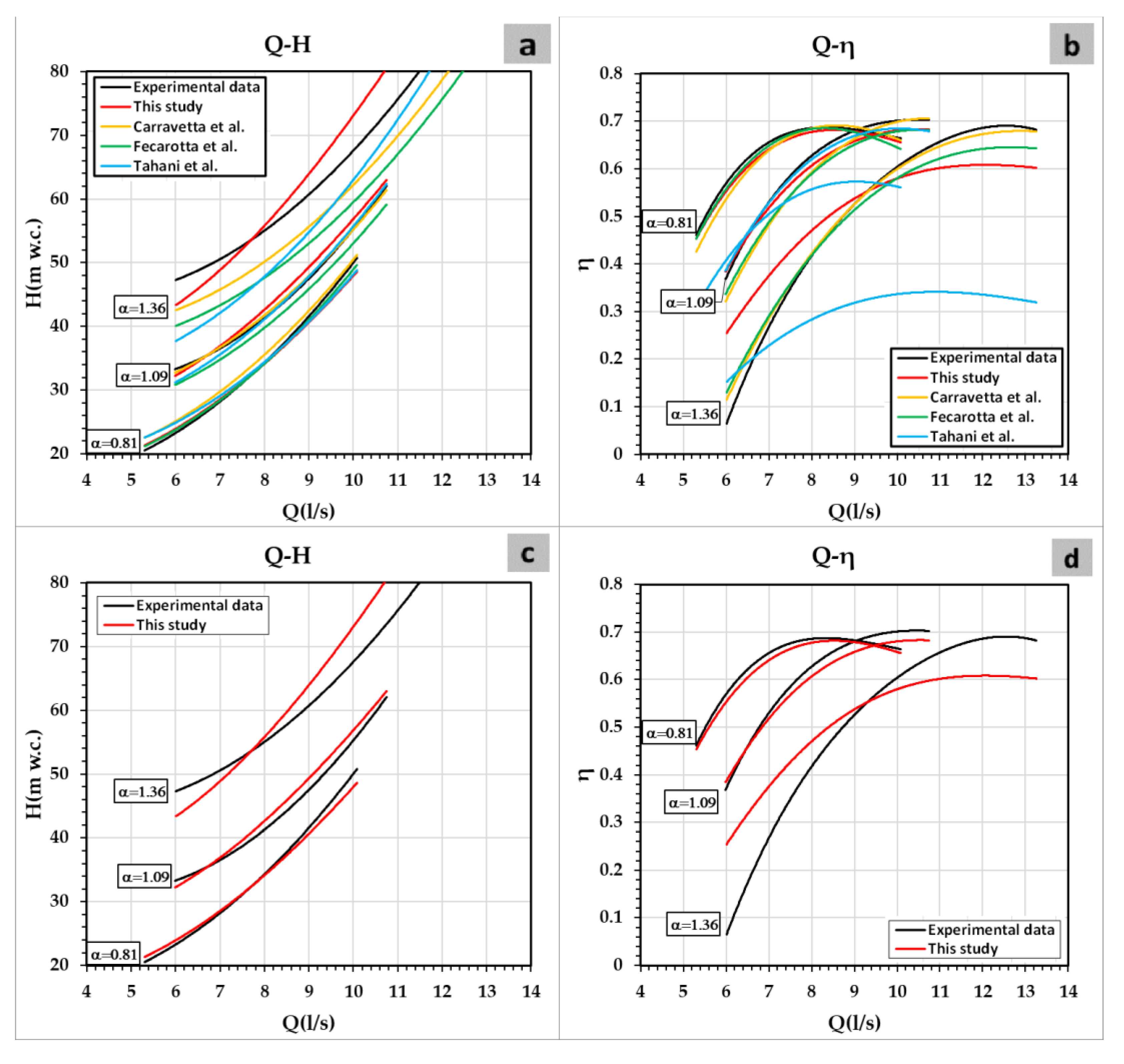
3.3. Proposed Functions vs. Other Published Functions

Once the relative errors of the selected function model (F6) were compared for each rotational speed of the different tested machine in the different proposed functions of head, efficiency, and power, the proposed expressions were compared with other expressions which have already been published in the literature.
This research proposes the following particular functions to define the characteristic curves of the machine according to expressions (21)–(23). The model F6 was chosen when head and efficiency curves should be estimated. F6 showed the lowest errors compared to the rest of the models. Moreover, this model contained the variation of the rotational speed ( α ) as well as the use of the ratio Q/QBEP, enabling us to measure the closeness to BEP. To calculate the power, F7 was chosen since it had the minimum error values, and it uses a simpler expression. The final expressions proposed herein are:
q = 0.1525 ( α Q Q B E P ) + 0.1958 ( Q Q B E P ) 2 0.0118 ( Q Q B E P ) 0.6429 α 2 + 1.8489 α 0.2241
h = 0.31070 ( α Q Q B E P ) + 0.3172 ( Q Q B E P ) 2 0.0546 ( Q Q B E P ) + 0.242 α 2 + 1.1708 α 0.3426
e = 0.8271 ( α Q Q B E P ) 0.3187 ( Q Q B E P ) 2 0.1758 ( Q Q B E P ) 1.035 α 2 + 1.1815 α + 0.5019
p = α 2.4762 ;
q = α 0.7439
The comparison concerns the model proposed in this research and four published proposals that are shown in Table 5.
Figure 5 shows the different values for error, when head, efficiency, and power were estimated using the proposed model (in black color, “this study”) and the rest of the published models. In all cases, the present proposed model presented the best results.
When head curve was analyzed, the error indexes (RMSE, MAD, and MRD) were reduced between 20 and 45% compared to the second-best model (Carravetta et al.). The BIAS value for this characteristic curve was −0.005, compared to the second-best model (0.048). Similar values were shown when the efficiency curve was compared. When efficiency errors were compared, RMS, MAD, and MRD were reduced by 33% compared to the second-best model, while BIAS was ten times lower than the second-best model. Finally, when the power errors were checked using the F7 model, the error indexes were reduced between 36 and 63% compared to the second-best model. Only when BIAS was checked, the second-best value was observed. Moreover, the F6 model was also compared to the rest of the proposed models for the power curve. This model (F6) showed good accuracy and the error indexes were 0.2209 (RMSE), 0.1884 (MAD), 0.0823 (MRD), and −0.097 (BIAS). All values were better than the second-best model, except for BIAS, which was the third-best value.
Finally, a visual comparison was carried out on the proposed model and the remaining models compared to an experimental PAT curve (Figure 6). To develop this comparison, the chosen PAT was a radial machine. The specific speed was 5.67 rpm (m, kW) and its nominal rotational speed was 1100 rpm. The best operation point of this machine was defined as 9.762 l/s and 51.267 m w.c., the efficiency being equal to 0.703 [24]
Figure 6a,b show the good accuracy of the proposed model compared to the rest of the models. This accuracy can be observed for each α value. Figure 6a shows the accuracy of the proposed study, other published models, and experimental data. All models showed good accuracy when the head curve was compared with the experimental data. However, this accuracy decreased in the rest of the models when α was higher than one. The accuracy of the proposed expressions was much better when the efficiency curves were compared. This visual accuracy, which can only be observed, is supported by analysis of errors indexes shown in Figure 5. In this graph, the proposed expressions reduced over 20% of the error of the other published methods. The mean reduction in the error was 60%. To improve this perception, Figure 6c,d show the comparison between the proposed model and the experimental data. In all cases, the accuracy was good but, when the α was between 0.8 and 1.2, the estimation of the curves showed excellent accuracy.

4. Conclusions

This research proposed a modification of the affinity laws (MOAL) of the hydraulic machines that are used as pumps working as turbines. This modification was established according to a new methodology, which was defined in this research. The research proposed an analysis with ten general expressions (polynomial and exponential), considering the most significant variables (the ratio of the rotational speed, α , and the ratio of Q and Q B E P ). Finally, a polynomial model (namely F6) depending on α and Q Q B E P was selected, when head and efficiency were estimated, and a potential model (F7) if the power is to be calculated directly. All proposed models exhibited good error indexes (RMSE, MAD, MRD, and BIAS) compared to the others, reducing the errors between 30 and 50% compared to the second-best model.
In addition, the proposed models were checked and compared to 15 different machines, which were tested by varying their rotational speed and its specific speed between 5 and 50 rpm (m, kW). The present model is based on 87 different curves and 56,450 operation points, using the largest database ever published.
The use of these models, which have excellent accuracy when α is between 0.8 and 1.2, is crucial to the development of mathematical models. These are of paramount importance to introduce the use of PATs when the manufacturer curve is not known. This is common when PATs are used, since the manufacturers do not publish these curves in their catalogue. Therefore, the inclusion of these equations will allow water managers to develop simulation tools, which can be introduced in the management of the water systems, improving the accuracy in their operation estimation. These models are expected to give a new impetus in the inclusion of the analysis tools when PATs operate at variable speed in water systems, and water modelers need mathematical expressions to develop simulations and operational limitations. Consequently, future works should be developed in which different procedures are proposed to establish the best variable operating strategy (VOS) in order to maximize the energy recovery using these expressions.

Author Contributions

Conceptualization, F.-J.S.-R. and M.P.-S., methodology, F.A.P.; software, V.H.; formal analysis, F.A.P.; writing—original draft preparation, F.A.P., F.-J.S.-R. and M.P.-S.; writing—review and editing, M.P.-S. and P.A.L.-J.; visualization, F.-J.S.-R. and M.P.-S.; supervision, P.A.L.-J. All authors have read and agreed to the published version of the manuscript.

Funding

This research received no external funding.

Institutional Review Board Statement

Not applicable.

Informed Consent Statement

Not applicable.

Data Availability Statement

Not applicable.

Conflicts of Interest

The authors declare no conflict of interest.

References

  1. Mangalekar, R.D.; Gumaste, K.S. Residential water demand modelling and hydraulic reliability in design of building water supply systems: A review. Water Supply 2021. [Google Scholar] [CrossRef]
  2. Bach, P.M.; Rauch, W.; Mikkelsen, P.S.; McCarthy, D.T.; Deletic, A. A critical review of integrated urban water modelling–Urban drainage and beyond. Environ. Model Softw. 2014, 54, 88–107. [Google Scholar] [CrossRef]
  3. Mousavi, S.N.; Bocchiola, D. A novel comparative statistical and experimental modeling of pressure field in free jumps along the apron of USBR Type I and II dissipation basins. Mathematics 2020, 8, 2155. [Google Scholar] [CrossRef]
  4. Raboaca, M.S.; Bizon, N.; Trufin, C.; Enescu, F.M. Efficient and secure strategy for energy systems of interconnected farmers′ associations to meet variable energy demand. Mathematics 2020, 8, 2182. [Google Scholar] [CrossRef]
  5. Puust, R.; Kapelan, Z.; Savic, D.A.; Koppel, T. A review of methods for leakage management in pipe networks. Urban Water J. 2010, 7, 25–45. [Google Scholar] [CrossRef]
  6. Vakilifard, N.; Anda, M.; Bahri, P.A.; Ho, G. The role of water-energy nexus in optimising water supply systems—Review of techniques and approaches. Renew. Sustain. Energy Rev. 2018, 82, 1424–1432. [Google Scholar] [CrossRef]
  7. Orouji, H.; Bozorg Haddad, O.; Fallah-Mehdipour, E.; Mariño, M.A. Modeling of water quality parameters using data-driven models. J. Environ. Eng. 2013, 139, 947–957. [Google Scholar] [CrossRef] [Green Version]
  8. Ramos, H.; Borga, A. Pumps as turbines: An unconventional solution to energy production. Urban Water 1999, 1, 261–263. [Google Scholar] [CrossRef]
  9. García, I.F.; Novara, D.; Mc Nabola, A. A model for selecting the most cost-effective pressure control device for more sustainable water supply networks. Water 2019, 11, 1297. [Google Scholar] [CrossRef] [Green Version]
  10. Pérez-Sánchez, M.; Sánchez-Romero, F.J.; Ramos, H.M.; López-Jiménez, P.A. Improved planning of energy recovery in water systems using a new analytic approach to PAT performance curves. Water 2020, 12, 468. [Google Scholar] [CrossRef] [Green Version]
  11. Pérez-Sánchez, M.; Sánchez-Romero, F.; Ramos, H.; López-Jiménez, P. Energy recovery in existing water networks: Towards greater sustainability. Water 2017, 9, 97. [Google Scholar] [CrossRef] [Green Version]
  12. Fecarotta, O.; Aricò, C.; Carravetta, A.; Martino, R.; Ramos, H.M. Hydropower Potential in Water Distribution Networks: Pressure Control by PATs. Water Resour Manag. 2015, 29, 699–714. [Google Scholar] [CrossRef]
  13. Quaranta, E.; Bonjean, M.; Cuvato, D.; Nicolet, C.; Dreyer, M.; Gaspoz, A.; Rey-Mermet, S.; Boulicaut, B.; Pratalata, L.; Pinelli, M.; et al. Hydropower case study collection: Innovative low head and ecologically improved turbines, hydropower in existing infrastructures, hydropeaking reduction, digitalization and governing systems. Sustainability 2020, 12, 8873. [Google Scholar] [CrossRef]
  14. Carravetta, A.; Conte, M.C.; Fecarotta, O.; Ramos, H.M. Evaluation of PAT performances by modified affinity law. Procedia Eng. 2014, 89, 581–587. [Google Scholar] [CrossRef] [Green Version]
  15. Suter, P. Representation of pump characteristics for calculation of water hammer. Sulzer Tech. Rev. 1966, 66, 45–48. [Google Scholar]
  16. Kougias, I.; Aggidis, G.; Avellan, F.; Deniz, S.; Lundin, U.; Moro, A.; Muntean, S.; Novara, D.; Perez-Diaz, J.I.; Quaranta, E.; et al. Analysis of emerging technologies in the hydropower sector. Renew. Sustain. Energy Rev. 2019, 113, 109257. [Google Scholar] [CrossRef]
  17. Novara, D.; McNabola, A. A model for the extrapolation of the characteristic curves of Pumps as Turbines from a datum best efficiency point. Energy Convers. Manag. 2018, 174, 1–7. [Google Scholar] [CrossRef]
  18. Shah, S.R.; Jain, S.V.; Patel, R.N.; Lakhera, V.J. CFD for centrifugal pumps: A review of the state-of-the-art. Procedia Eng. 2013, 51, 715–720. [Google Scholar] [CrossRef] [Green Version]
  19. Carravetta, A.; Del Giudice, G.; Fecarotta, O.; Ramos, H. Pump as Turbine (PAT) design in water distribution network by system effectiveness. Water 2013, 5, 1211–1225. [Google Scholar] [CrossRef] [Green Version]
  20. Iliev, I.; Trivedi, C.; Dahlhaug, O.G. Variable-speed operation of Francis turbines: A review of the perspectives and challenges. Renew. Sustain. Energy Rev. 2019, 103, 109–121. [Google Scholar] [CrossRef]
  21. Singh, P. Optimization of the Internal Hydraulic and of System Design in Pumps as Turbines with Field Implementation and Evaluation. Ph.D. Thesis, Karlsruhe Institute of Technology, Karlsruhe, Germany, 3 June 2005. [Google Scholar]
  22. Yang, S.S.; Derakhshan, S.; Kong, F.Y. Theoretical, numerical and experimental prediction of pump as turbine performance. Renew. Energy 2012, 48, 507–513. [Google Scholar] [CrossRef]
  23. Rossi, M.; Nigro, A.; Renzi, M. Experimental and numerical assessment of a methodology for performance prediction of Pumps-as-Turbines (PaTs) operating in off-design conditions. Appl. Energy 2019, 248, 555–566. [Google Scholar] [CrossRef]
  24. Novara, D.; Carravetta, A.; McNabola, A.; Ramos, H.M. Cost model for pumps as turbines in run-of-river and in-pipe microhydropower applications. J. Water Resour. Plan. Manag. 2019, 145, 04019012. [Google Scholar] [CrossRef]
  25. Derakhshan, S.; Nourbakhsh, A. Experimental study of characteristic curves of centrifugal pumps working as turbines in different specific speeds. Exp. Therm. Fluid Sci. 2008, 32, 800–807. [Google Scholar] [CrossRef]
  26. Carravetta, A.; del Giudice, G.; Fecarotta, O.; Ramos, H. PAT design strategy for energy recovery in water distribution networks by electrical regulation. Energies 2013, 6, 411–424. [Google Scholar] [CrossRef] [Green Version]
  27. Pérez-Sánchez, M.; López-Jiménez, P.A.; Ramos, H.M. Modified affinity laws in hydraulic machines towards the best efficiency line. Water Resour. Manag. 2018, 32, 829–844. [Google Scholar] [CrossRef] [Green Version]
  28. Tahani, M.; Kandi, A.; Moghimi, M.; Houreh, S.D. Rotational speed variation assessment of centrifugal pump-as-turbine as an energy utilization device under water distribution network condition. Energy 2020, 213, 118502. [Google Scholar] [CrossRef]
  29. Mataix, C. Turbomáquinas Hidráulicas; Universidad Pontificia Comillas: Madrid, Spain, 2009. [Google Scholar]
  30. Morrison, G.; Yin, W.; Agarwal, R.; Patil, A. Development of modified affinity law for centrifugal pump to predict the effect of viscosity. J. Sol. Energy Eng. Trans. ASME. 2018, 140. [Google Scholar] [CrossRef]
  31. Fecarotta, O.; Carravetta, A.; Ramos, H.M.; Martino, R. An improved affinity model to enhance variable operating strategy for pumps used as turbines. J. Hydraul. Res. 2016, 1686, 1–10. [Google Scholar] [CrossRef]
  32. KSB. PATs Curves. Catalogue. Available online: https://www.ksb.com/ksb-en/ (accessed on 5 November 2019).
  33. Jain, S.V.; Swarnkar, A.; Motwani, K.H.; Patel, R.N. Effects of impeller diameter and rotational speed on performance of pump running in turbine mode. Energy Convers. Manag. 2015, 89, 808–824. [Google Scholar] [CrossRef]
  34. Nygren, L. Hydraulic Energy Harvesting with Variable-Speed-Driven Centrifugal Pump as Turbine. Ph.D. Thesis, Lappeenrtanta University of Technology, Lappeenranta, Finland, 2017. [Google Scholar]
  35. Abazariyan, S.; Rafee, R.; Derakhshan, S. Experimental study of viscosity effects on a pump as turbine performance. Renew. Energy 2018, 127, 539–547. [Google Scholar] [CrossRef]
  36. Kramer, M.; Terheiden, K.; Wieprecht, S. Pumps as turbines for efficient energy recovery in water supply networks. Renew. Energy 2018, 122, 17–25. [Google Scholar] [CrossRef] [Green Version]
  37. Delgado, J.; Ferreira, J.P.; Covas, D.I.C.; Avellan, F. Variable speed operation of centrifugal pumps running as turbines. Experimental investigation. Renew. Energy 2019, 142, 437–450. [Google Scholar] [CrossRef]
  38. Stefanizzi, M.; Torresi, M.; Fortunato, B.; Camporeale, S.M. Experimental investigation and performance prediction modeling of a single stage centrifugal pump operating as turbine. Energy Procedia 2017, 126, 589–596. [Google Scholar] [CrossRef]
  39. Postacchini, M.; Darvini, G.; Finizio, F.; Pelagalli, L.; Soldini, L.; Di Giuseppe, E. Hydropower generation through Pump as Turbine: Experimental study and potential application to small-scale WDN. Water 2020, 12, 958. [Google Scholar] [CrossRef] [Green Version]
  40. Pugliese, F.; De Paola, F.; Fontana, N.; Giugni, M.; Marini, G. Experimental characterization of two Pumps as Turbines for hydropower generation. Renew. Energy 2016, 99, 180–187. [Google Scholar] [CrossRef]
Figure 1. Methodology proposed to derive the expressions (m is the number of experimental machines, N is the maximum number of the tested machine).
Mathematics 09 00860 g001
Figure 2. Congruence parabolas for the different values and rotational speeds when modified affinity laws (MOAL) is applied.
Mathematics 09 00860 g002
Figure 3. (a) Definition of head as a function of the flow for different rotational speeds; (b) Definition of the efficiency as a function of the flow for different rotational speeds considering the VOS area.
Mathematics 09 00860 g003
Figure 4. Error values when power is determined: (a) root mean square error (RMSE) (b) mean absolute deviation (MAD); (c) mean relative deviation (MRD), and (d) absolute value of BIAS.
Mathematics 09 00860 g004
Figure 5. Error values for head, efficiency, and power, when the models are compared.
Mathematics 09 00860 g005
Figure 6. (a) Head curve comparison between proposed model, experimental data, and rest of published models; (b) Efficiency curve comparison between proposed model, experimental data, and rest of published models; (c) Head curve between proposed model and experimental curve; (d) Efficiency curve between proposed model and experimental curve.
Mathematics 09 00860 g006
Table 1. Proposed functions to be analyzed.
Function Model (FM) Polynomial   Function   ( from   F 1 to   F 6 ) :
N P = β 1 ( α Q Q B E P ) + β 2 ( Q Q B E P ) 2 + β 3 ( Q Q B E P ) + β 4 α 2 + β 5 α + β 6
Exponential   Function   ( from   F 7 to   F 10 ) :
N P = ( Q Q B E P ) β 3 α β 5 · e x p β 6
F 1 N P = β 4 α 2 + β 5 α
F 2 N P = β 4 α 2 + β 5 α + β 6
F 3 N P = β 2 ( Q Q B E P ) 2 + β 4 α 2 + β 5 α
F 4 N P = β 2 ( Q Q B E P ) 2 + β 4 α 2 + β 5 α + β 6
F 5 N P = β 1 ( α Q Q B E P ) + β 2 ( Q Q B E P ) 2 + β 3 ( Q Q B E P ) + β 4 α 2 + β 5 α
F 6 N P = β 1 ( α Q Q B E P ) + β 2 ( Q Q B E P ) 2 + β 3 ( Q Q B E P ) + β 4 α 2 + β 5 α + β 6
F 7 N P = α β 5
F 8 N P = α β 5 · e x p β 6
F 9 N P = ( Q Q B E P ) β 3 α β 5
F 10 N P = ( Q Q B E P ) β 3 α β 5 · e x p β 6
* NP is the non-dimensional parameter. It can be h ,   q ,   e , h q 2 , h e q 2 .
Table 2. Characteristics of the used pumps working as turbines (PATs).
IDRef. n s t   ( m ,   kW ) n 0   ( rpm ) D (mm) Q B E P   ( l / s ) H B E P
(m w.c.)
η B E P RSIPAP
1[32]20.661020139346141440.61547662393
2[33]28.34120020024,46012,4370.59676213812
325.57110022522,29511,9410.71478515646
426.43110025023,73111,9100.76677665086
5[34]17.68120021016,75518,1260.71868464377
627.0380026527,32283050.80056802997
725.44120025528,39215,8590.71565803035
8[35]13.651200139490611,2830.54337141937
9[36]5.671100193976251,2670.70366803514
10[37]31.16300012717,98530,2880.69568024535
1120.97300015817,97551,3550.72767774516
1250.71270012736,90922,2070.70576094139
13[38]21.75100041995,59134,4280.79547452595
14[39]13.841250175899017,5250.62268043020
15[40]33.1290018950,05052,8490.64677084848
Total8710,94956,450
RS, number of experimental curves, which were tested for different rotational speeds; IP, number of interpolated parabolas using the experimental curves for each rotational speed; AP, number of analyzed points.
Table 3. Values of the different β i for each proposed function model and considering the different non-dimensional parameters.
qp
FMR2 β 1 β 2 β 3 β 4 β 5 β 6 FMR2 β 1 β 2 β 3 β 4 β 5 β 6
F 1 0.9945------−0.46031.4250-- F 1 0.9133------0.44470.4063--
F 2 0.8630------−0.75382.0117−0.2765 F 2 0.6836------−0.84232.9793−1.2124
F 3 0.9955--0.1112--−0.45661.3510-- F 3 0.9244--0.3783--0.45740.1547--
F 4 0.8802--0.0925--−0.68671.8224−0.2163 F 4 0.7109--0.2897--−0.63252.3865−1.0239
F 5 0.9956−0.01090.2984−0.2918−0.55491.5705-- F 5 0.93572.09260.4300−2.2315−1.09841.8245--
F 6 0.8809−0.15250.1958−0.0118−0.64291.8489−0.2241 F 6 0.72971.67240.1255−1.4005−1.35962.6509−0.6651
F 7 0.8310--------0.7439-- F 7 0.8098--------2.4762--
F 8 0.8243--------0.6796−0.0540 F 8 0.8019--------2.2406−0.1978
F 9 0.8949----0.1847--0.5541-- F 9 0.8825----0.6644--1.7937--
F 10 0.8567----0.1675--0.5617−0.0085 F 10 0.8374----0.5858--1.8282−0.0388
hh/q2
FMR2 β 1 β 2 β 3 β 4 β 5 β 6 FMR2 β 1 β 2 β 3 β 4 β 5 β 6
F 1 0.9910------0.50720.4588-- F 1 0.9781------−0.51181.6305--
F 2 0.9474------0.09431.2844−0.3890 F 2 0.7375------1.0476−1.48701.4690
F 3 0.9919--0.1161--0.51110.3816-- F 3 0.9811--−0.2347--−0.51961.7866--
F 4 0.9506--0.0874--0.15761.1055−0.3321 F 4 0.7639--−0.1139--0.9651−1.25381.3948
F 5 0.9922−0.09420.4740−0.48280.37650.7450-- F 5 0.9862−1.5078−0.47061.92960.71430.3415--
F 6 0.9512−0.31070.3172−0.05460.24201.1708−0.3426 F 6 0.7780−0.69020.12180.31271.2224−1.26651.2940
F 7 0.9653--------1.7017-- F 7 0.2070--------0.2140--
F 8 0.9620--------1.6646−0.0312 F 8 0.4018--------0.30550.0768
F 9 0.9734----0.1392--1.5587-- F 9 0.5060----−0.2302--0.4505--
F 10 0.9684----0.1689--1.54570.0147 F 10 0.4786----−0.1660--0.42230.0317
ehe/q2
FMR2 β 1 β 2 β 3 β 4 β 5 β 6 FMR2 β 1 β 2 β 3 β 4 β 5 β 6
F 1 0.9796------−1.20392.1823-- F 1 0.9792------−0.82551.8427--
F 2 0.2391------−0.82351.42190.3583 F 2 0.1508------−0.17060.53360.6169
F 3 0.9798--0.0535--−1.20212.1467-- F 3 0.9792--−0.0236--−0.82631.8584--
F 4 0.2602--0.0896--−0.75861.23850.4167 F 4 0.1538--0.0316--−0.14780.46900.6374
F 5 0.98030.5100−0.54850.4514−1.23211.8052-- F 5 0.98010.5319−0.82800.7565−0.75721.2873--
F 6 0.28320.8271−0.3187−0.1758−1.03501.18150.5019 F 6 0.19120.9930−0.4939−0.1555−0.47060.38040.7298
F 7 0.0017--------0.0306-- F 7 0.1753--------0.2447--
F 8 0.0214--------−0.1036−0.1127 F 8 0.1160--------0.2019−0.0359
F 9 0.2677----0.3404--−0.3191-- F 9 0.2197----0.1102--0.1315--
F 10 0.1019----0.2494--−0.2791−0.0450 F 10 0.1288----0.0834--0.1432−0.0132
Table 4. Average error indexes for the different characteristic curves using the defined M O A L .
Expression (21)Expression (22)Expression (23)
H = h ( A + B Q q + C ( Q q ) 2 ) η = e   ( E 4 ( Q q ) 4 + E 3 ( Q q ) 3 + E 2 ( Q q ) 2 + E 1 ( Q q ) + E 0 ) P = p   ( P 4 ( Q q ) 4 + P 3 ( Q q ) 3 + P 2 ( Q q ) 2 + P 1 ( Q q ) + P 5 )
FMRMSEMADMRDBIASFMRMSEMADMRDBIASFMRMSEMADMRDBIAS
F 1 0.6869
(6)
0.5733
(6)
0.0325
(8)
0.1695
(7)
F 1 0.0596
(8)
0.0486
(8)
0.1161
(8)
0.0198
(9)
F 1 0.2666
(8)
0.221
(9)
0.1467
(9)
0.0678
(8)
F 2 0.7234
(9)
0.6007
(9)
0.0296
(5)
0.1054
(6)
F 2 0.0656
(10)
0.0493
(10)
0.1185
(10)
0.0173
(7)
F 2 0.2391
(6)
0.1983
(7)
0.1313
(7)
0.049
(4)
F 3 0.6099
(3)
0.5109
(1)
0.0286
(3)
0.0272
(5)
F 3 0.0487
(4)
0.042
(6)
0.1139
(7)
0.004
(4)
F 3 0.3341
(10)
0.259
(10)
0.1626
(10)
0.1305
(10)
F 4 0.6535
(5)
0.5448
(5)
0.0274
(2)
0.0264
(4)
F 4 0.0469
(2)
0.0381
(3)
0.1015
(2)
0.0009
(1)
F 4 0.2732
(9)
0.213
(8)
0.1398
(8)
0.0222
(1)
F 5 0.6077
(2)
0.5113
(2)
0.0289
(4)
0.0026
(2)
F 5 0.0494
(5)
0.0424
(7)
0.1115
(6)
0.0052
(5)
F 5 0.2314
(5)
0.1775
(5)
0.1216
(5)
0.0646
(6)
F 6 0.6075
(1)
0.5154
(3)
0.0266
(1)
0.005
(3)
F 6 0.0397
(1)
0.0331
(1)
0.0883
(1)
0.0027
(3)
F 6 0.2472
(7)
0.194
(6)
0.1272
(6)
0.0654
(7)
F 7 0.6101
(4)
0.5186
(4)
0.0302
(6)
0.3739
(9)
F 7 0.054
(7)
0.0419
(5)
0.1033
(3)
0.0016
(2)
F 7 0.1169
(1)
0.1017
(1)
0.0858
(1)
0.023
(2)
F 8 0.6979
(7)
0.5911
(8)
0.0332
(9)
0.0021
(1)
F 8 0.0652
(9)
0.049
(9)
0.111
(5)
0.0222
(10)
F 8 0.174
(4)
0.1471
(4)
0.0886
(2)
0.1127
(9)
F 9 0.7697
(10)
0.6154
(10)
0.0349
(10)
0.4324
(10)
F 9 0.0506
(6)
0.0414
(4)
0.1174
(9)
0.0182
(8)
F 9 0.1486
(2)
0.13
(2)
0.0964
(4)
0.0364
(3)
F 10 0.7085
(8)
0.5847
(7)
0.0321
(7)
0.216
(8)
F 10 0.047
(3)
0.0379
(2)
0.1107
(4)
0.0064
(6)
F 10 0.1504
(3)
0.1345
(3)
0.0942
(3)
0.0629
(5)
The ranking of the Fi when the error indexes are compared from (1) to (9) as indicated.
Table 5. Methods used for the comparison.
MethodReferencehqp η
Carravetta et al. (2014)[14] 1.0253 α 1.5615 1.0323 α 0.7977 0.9741 α 2.3207 0.4013 α 2 + 0.845 α + 0.5606
Fecarotta et al. (2016)[12] 0.972 α 1.603 1.004 α 0.825 -- 0.317 α 2 + 0.587 α + 0.707
Pérez-Sánchez et al. (2018)[27] 1.89 α 2 1.54 α + 0.74 1.08 α 0.7 4.59 α 2 6.33 α + 2.50 0.36 α 2 0.69 α + 0.66
Tahani et al. (2020)[28] 0.9962 α 1.0851 0.9974 α 0.3651 0.9767 α 1.4888 4.3506 α 2 + 8.8879 α 3.544
Publisher’s Note: MDPI stays neutral with regard to jurisdictional claims in published maps and institutional affiliations.

