An Exhaustive Power Comparison of Normality Tests

1. Introduction

A priori information about data distribution is not always known. In those cases, hypothesis testing can help to find a reasonable assumption about the distribution of data. Based on assumed data distribution, one can choose appropriate methods for further research. The information about data distribution can be useful in a number of ways, for example:

• it can provide insights about the observed process;
• parameters of model can be inferred from the characteristics of data distributions; and
• it can help in choosing more specific and computationally efficient methods.

Statistical methods often require data to be normally distributed. If the assumption of normality is not satisfied, the results of these methods will be inappropriate. Therefore, the presumption of normality is strictly required before starting the statistical analysis. Many tests have been developed to check this assumption. However, tests are defined in various ways and thus react to abnormalities, present in a data set, differently. Therefore, the choice of goodness-of-fit test remains an important problem.

$$\begin{gathered} H_0:The distribution is normal, \\ {H}_A:The distribution is not normal. \end{gathered}$$

For these reasons, this study examines the issue of testing the goodness-of-fit hypotheses. The goodness-of-fit null and alternative hypotheses are defined as:

A total of 40 tests were applied to analyze the problem of testing the goodness-of-fit hypothesis. The tests used in this study were developed between 1900 and 2016. In the early 19th century, Karl Pearson published an article defining the chi-square test [1]. This test is considered as the basis of modern statistics. Pearson was the first to examine the goodness-of-fit assumption that the observations $x_i$can be distributed according to the normal distribution, and concluded that, in the limit as $n$ becomes large, $X^2$ follows the chi-square distribution with $k-1$ degrees of freedom. The statistics for this test are defined in Section 2.1. Another popular test for testing the goodness-of-fit hypothesis is the Kolmogorov and Smirnov test [2]. This test statistic quantifies a distance between the empirical distribution function of the sample and the cumulative distribution function of the reference distribution [3]. The Anderson and Darling test is also often used in practice [4]. This test assesses whether a sample comes from a specified distribution [3]. The end of 19th century and the beginning of 20th century was a successful period for the development of goodness-of-fit hypothesis test criteria and their comparison studies [5,6,7,8,9,10,11,12,13,14,15,16,17,18,19].

In 2010, Xavier Romão et al. conducted a comprehensive study comparing the power of the goodness-of-fit hypothesis tests [20]. In the study, 33 normality tests were applied to samples of different sizes, taking into account the significance level $\alpha$ and many symmetric, asymmetric, and modified normal distributions. The researchers found that the most powerful of the selected normality tests for the symmetric group of distributions were Coin ${\beta }_3^2$, Chen–Shapiro, Bonett–Seier, and Gel–Miao–Gastwirth tests; for the asymmetric group of distributions, Zhang–Wu $Z_C$ and $Z_A$, and Chen–Shapiro; while the Chen–Shapiro, Barrio–Cuesta-Albertos–Matrán–Rodríguez-Rodríguez, and Shapiro–Wilk tests were the most powerful for the group of modified normal distributions.

In 2015, Adefisoye et al. compared 18 normality tests for different sample sizes for symmetric and asymmetric distribution groups [3]. The results of the study showed that the Kurtosis test was the most powerful for a group of symmetric data distributions and the Shapiro–Wilk test was the most powerful for a group of asymmetric data distributions.

The main objective of this study is to perform a comparative analysis of the power of the most commonly used tests for testing the goodness-of-fit hypothesis. The procedure described in Section 3 was used to calculate the power of the tests.

Scientific novelty—the comparative analysis of test power was carried out using different methods for goodness-of-fit in the case of many different types of challenges to curve tests. The goodness-of-fit tests have been selected as representatives of popular techniques, which have been analyzed by other researchers experimentally. We have proposed a new kernel function and its usage in an N-metric-based test. The uniqueness of the kernel function is that its shape is chosen in such a way that the shift arising in the formation of the test is eliminated by using sample values.

The rest of the paper is organized as follows. Section 2 provides descriptions of the 40 goodness-of-fit hypothesis tests and the procedure for calculating the power of the tests. The samples generated from 15 distributions are given in Section 4. Section 5 presents and discusses the results of a simulation modeling study. Finally, Section 6 concludes the results.

2. Statistical Methods

In this section, the most popular tests for normality are overviewed.

2.1. Chi-Square Test (CHI2)

In 1900, Karl Pearson introduced the chi-square test [1]. The statistic of the test is defined as:

$${\chi }^2={\displaystyle \sum }_{i=1}^k\frac{{(O_i-E_i)}^2}{E_i},$$

(1)

where $O_i$ is the observed frequency and $E_i$ is the expected frequency.

2.2. Kolmogorov–Smirnov (KS)

In 1933, Kolmogorov and Smirnov proposed the KS test [2]. The statistic of the test is defined as:

$$\begin{gathered} {\chi }^2=D^{+}=\max \left\{\left(\frac{i}{n}\right)-z_i\right\}, 1\le i\le n; \\ {D}^{-}=\max \left\{z_i-\frac{i-1}{n}\right\}, 1\le i\le n; \\ D=\max \left(D^{+},D^{-} \right), \end{gathered}$$

(2)

where $z_i$ is the cumulative probability of standard normal distribution and $D$ is the difference between observed and expected values.

2.3. Anderson–Darling (AD)

In 1952, Anderson and Darling developed a variety of the Kolmogorov and Smirnov tests [4]. This test is more powerful than the Kolmogorov and Smirnov test. The statistic of the test is defined as:

$$A^2=-n-{\displaystyle \sum }_{i=1}^n\frac{2i-1}{n}\left(\ln \left(F\left(x_i\right)\right)+\ln (1-F\left(x_{n+1-i}\right))\right),$$

(3)

where $F\left(x_i\right)\mathrm{is}$the value of the distribution function at point $x_i$ and $n\mathrm{is}\mathrm{the}$empirical sample size.

2.4. Cramer–Von Mises (CVM)

In 1962, Cramer proposed the Cramer–von Mises test. This test is an alternative to the Kolmogorov and Smirnov test [21]. The statistic of the test is defined as:

$$CM=\frac{1}{12n}+{\displaystyle \sum }_{i=1}^n{\left(Z_i-\frac{2i-1}{2n}\right)}^2,$$

(4)

where $Z_i$is the cumulative distribution function of the specified distribution $Z_i=X_{\left(i\right)}-\overline{X}/S, \overline{ \mathrm{and} X}$and $S$ are the sample mean and sample standard deviation.

2.5. Shapiro–Wilk (SW)

In 1965, Shapiro and Wilk formed the original test [22]. The statistic of the test is defined as:

$$W=\frac{{\left({{\displaystyle \sum }}_{i=1}^n{a}_i{x}_{\left(i\right)}\right)}^2}{{\left({{\displaystyle \sum }}_{i=1}^n{x}_i-\overline{x}\right)}^2},$$

(5)

where$x_{\left(i\right)}$ is the $i^{th}$ order statistic, $\overline{x}$ is the sample mean, and $a_i$constants obtained:

$$a_i=\left(a_1,\dots ,a_n\right)=\frac{m^T{V}^{-1}}{{\left(m^T{V}^{-1}{V}^{-1}m\right)}^{1/2}} ,$$

where $m=(m_1,\dots ,m_n){}^T$ are the expected values of the order statistics of independent and identically distributed random variables sampled from the standard normal distribution and $V$ is the covariance matrix of those order statistics.

2.6. Lilliefors (LF)

In 1967, Lilliefors modified the Kolmogorov and Smirnov test [23]. The statistic of the test is defined as:

$$T=\underset{x}{\sup }\left|F^{*}\left(x\right)-S\left(x\right)\right|,$$

(6)

where $F^{*}\left(x\right) \mathrm{is}$the standard normal distribution function and $S\left(x\right) \mathrm{is}$the empirical distribution function of the $z_i$ values.

2.7. D’Agostino (DA)

In 1971, D’Agostino introduced the test for testing the goodness-of-fit hypothesis, which is an extension of the Shapiro–Wilk test [8]. The test proposed by D’Agostino does not need to define a weight vector. The statistic of the test is defined as:

$$D=\frac{{{\displaystyle \sum }}_{i=1}^n\left(i-\left(n+1\right)/2\right)·x_{\left(i\right)}}{n^2·\sqrt{m_2}},$$

(7)

where $m_2$ is the second central moment that is defined as:

$$m_2=n^{-1}{\displaystyle \sum }_{i=1}^n{\left(x_i-\overline{x}\right)}^2.$$

2.8. Shapiro–Francia (SF)

In 1972, Shapiro and Francia simplified the Shapiro and Wilk test and developed the Shapiro and Francia test, which is computationally more efficient [24]. The statistic of the test is defined as:

$$W_{SF}=\frac{{\left({{\displaystyle \sum }}_{i=1}^n{m}_i{x}_i\right)}^2}{{\left({{\displaystyle \sum }}_{i=1}^n{x}_i-\overline{x}\right)}^2{{\displaystyle \sum }}_{i=1}^n{m}_i^2},$$

(8)

where $m_i\mathrm{is}$ the expected values of the standard normal order statistics.

2.9. D’Agostino–Pearson (DAP)

In 1973–1974, D’Agostino and Pearson proposed the D’Agostino and Pearson test [25]. The statistic of the test is defined as:

$$DP=\frac{{{\displaystyle \sum }}_{i=1}^n\left(i-\left(n+1\right)/2\right)x_{\left(i\right)}}{n^2\sqrt{m_2}},$$

(9)

where $n$ is the size of sample and $m_2$ is the sample variance of order statistics.

2.10. Filliben (Filli)

In 1975, Filliben defined the probabilistic correlation coefficient $r$ as a test for the goodness-of-fit hypothesis [26]. This test statistic is defined as:

$$r=\frac{{{\displaystyle \sum }}_{i=1}^n{x}_{\left(i\right)}·M_{\left(i\right)}}{\sqrt{{{\displaystyle \sum }}_{i=1}^n{M}_{\left(i\right)}^2}·\sqrt{\left(n-1\right)·{\sigma }^2}},$$

(10)

where ${\sigma }^2\mathrm{is}$ the variance,$M_{\left(i\right)}={\mathsf{\Phi }}^{-1}\left(m_{\left(i\right)}\right)$, when $m_{\left(i\right)} \mathrm{is}$the estimated median values of the order statistics, each $m_{\left(i\right)}$ is obtained by:

$$m_{\left(i\right)}=\{\begin{array}{c}1-{0.5}^{\left(\frac{1}{n}\right)} i=1,\\ \frac{\left(i-0.3175\right)}{\left(n+0.365\right)} 1<i<n,\\ {0.5}^{\left(\frac{1}{n}\right)} i=n.\end{array}$$

2.11. Martinez–Iglewicz (MI)

In 1981, Martinez and Iglewicz proposed a normality test based on the ratio of two estimators of variance, where one of the estimators is the robust biweight scale estimator $S_b^2$ [27]:

$$S_b^2=\frac{n·{{\displaystyle \sum }}_{\left|{\tilde{z}}_i\right|<1}{\left(x_i-M\right)}^2{\left(1-{\tilde{z}}_i^2\right)}^4}{{\left[{{\displaystyle \sum }}_{\left|{\tilde{z}}_i\right|<1}\left(1-{\tilde{z}}_i^2\right)\left(1-5{\tilde{z}}_i^2\right)\right]}^2},$$

where $M$ is the sample median, ${\tilde{z}}_i=\left(x_i-M\right)/\left(9A\right)$, with $A$ being the median of $\left|x_i-M\right|$.

This test statistic is then given by:

$$I_n=\frac{{{\displaystyle \sum }}_{i=1}^n{\left(x_i-M\right)}^2}{\left(n-1\right)·S_b^2}.$$

(11)

2.12. Epps–Pulley (EP)

In 1983, Epps and Pulley proposed a test statistic based on the following weighted integral [28]:

$$T_{EP}={{\displaystyle \int }}_{-\infty }^{\infty }{\left|{\phi }_n\left(t\right)-{\widehat{\phi }}_0\left(t\right)\right|}^{2}dG\left(t\right),$$

where ${\phi }_n\left(t\right)$ is the empirical characteristic function and $G\left(t\right)$ is an adequate function chosen according to several considerations. By setting $dG\left(t\right)=g\left(t\right)dt$ and selecting:

$$g\left(t\right)=\sqrt{m_2/2\pi }·exp\left(-0.5m_2{t}^2\right)$$

the following statistic is obtained:

$$T_{EP}=1+\frac{n}{\sqrt{3}}+\frac{2}{n}{\displaystyle \sum }_{k=2}^n{\displaystyle \sum }_{j=1}^{k-1}\exp \left(\left(-{\left(x_j-x_k\right)}^2\right)/2m_2\right)-\sqrt{2}{\displaystyle \sum }_{j=1}^n\exp \left(\left(-{\left(x_j-\overline{x}\right)}^2\right)/4m_2\right),$$

(12)

where $m_2 \mathrm{is}$the second central moment.

2.13. Jarque–Bera (JB)

In 1987, Jarque and Bera proposed a test [29] with statistic defined as:

$$JB=\frac{n}{6}\left(s+\frac{{\left(k-3\right)}^2}{4}\right),$$

(13)

where $s=\frac{m_3^2}{m_2^3}$ and $k=\frac{m_4}{m_2^3}$ are the sample skewness and kurtosis.

2.14. Hosking ($H_1-H_3)$

In 1990, Hosking and Wallis proposed the first Hosking test [5]. This test statistic is defined as:

$$H_i=\frac{V_i-{\mu }_V}{{\sigma }_V},$$

(14)

where ${\mu }_V$ and ${\sigma }_V$ are the mean and standard deviation of number of simulation data values of $V.$ $V_i$ is calculated as:

$$V_1=\sqrt{\frac{{{\displaystyle \sum }}_{i=1}^N{n}_i{\left(t^{\left(i\right)}-t^R\right)}^2}{{{\displaystyle \sum }}_{i=1}^N{n}_i}}, V_2={\displaystyle \sum }_{i=1}^N{n}_i\frac{\sqrt{{\left(t^{\left(i\right)}-t^R\right)}^2+{\left(t_3-t_3^R\right)}^2}}{{{\displaystyle \sum }}_{i=1}^N{n}_i},$$

$$V_3={\displaystyle \sum }_{i=1}^N{n}_i\frac{\sqrt{{\left(t_3^{\left(i\right)}-t_3^R\right)}^2+{\left(t_4^{\left(i\right)}-t_4^R\right)}^2}}{{{\displaystyle \sum }}_{i=1}^N{n}_i}, t^R=\frac{{{\displaystyle \sum }}_{i=1}^N{n}_i{t}^{\left(i\right)}}{{{\displaystyle \sum }}_{i=1}^N{n}_i},$$

where $t^{\left(i\right)} \mathrm{is}\mathrm{the}$ coefficient of variation of the L-moment ratio, $t_3^{\left(i\right)}\mathrm{is}\mathrm{the}$ coefficient of skewness of the L- moment, and $t_4^{\left(i\right)}$ is the coefficient of kurtosis of the L- moment.

2.15. Cabaña–Cabaña (CC1-CC2)

In 1994, Cabaña and Cabaña proposed the CC1 and CC2 tests [6]. The CC1 ($T_{S,l}$) and CC2 ($T_{K,l}$), respectively, are defined as:

$$T_{S,l}=\max \left| w_{S,l}\left(x\right)\right|, T_{K,l}= \max \left| w_{K,l}\left(x\right)\right|,$$

(15)

where$w_{S,l}\left(x\right)$and $w_{K,l}\left(x\right)$approximate transformed estimated empirical processes sensitive to changes in skewness and kurtosis and are defined as:

$$\begin{gathered} w_{S,l}=\mathsf{\Phi }\left(x\right)·{\overline{H}}_3-\varphi \left(x\right)·{\displaystyle \sum }_{j=1}^l\frac{1}{\sqrt{j}}{H}_{j-1}\left(x\right)·{\overline{H}}_{j+3}, \\ w_{K,l}=-\varphi \left(x\right)·{\overline{H}}_3+\left[\mathsf{\Phi }\left(x\right)-x·\varphi \left(x\right)\right]·{\overline{H}}_4-\varphi \left(x\right)·{\displaystyle \sum }_{j=2}^l\left(\sqrt{\frac{j}{j-1}}{H}_{j-2}\left(x\right)·H_j\left(x\right)\right)·{\overline{H}}_{j+3}, \end{gathered}$$

where $l \mathrm{is}$a dimensionality parameter, $\mathsf{\Phi }\left(x\right) \mathrm{is}$the probability density function of the standard normal distribution, $H_j(·) \mathrm{is}$the $j$th order normalized Hermite polynomial, and ${\overline{H}}_j\mathrm{is}$the$j$th order normalized mean of the Hermite polynomial defined as: ${\overline{H}}_j=\frac{1}{\sqrt{n}}{\displaystyle \sum }_{i=1}^n{H}_j\left(x_i\right).$

2.16. The Chen–Shapiro Test (ChenS)

In 1995, Chen and Shapiro introduced an alternative test statistic based on normalized spacings and defined as [9]:

$$CS=\frac{1}{\left(n-1\right)·s}{\displaystyle \sum }_{i=1}^{n-1}\frac{x_{\left(i+1\right)}-x_{\left(i\right)}}{M_{i+1}-M_i},$$

(16)

where $M_i \mathrm{is}$the $i$th quantile of a standard normal distribution.

2.17. Modified Shapiro-Wilk (SWRG)

In 1997, Rahman and Govindarajulu proposed a modification to the Shapiro–Wilk test [8]. This test statistic is simpler to compute and relies on a new definition of the weights using the approximations to $m$ and $V$. Each element $a_i$of the weight vector is given as:

$$a_i=-\left(n+1\right)\left(n+2\right)\varphi \left(m_i\right)\left[m_{i-1}\varphi \left(m_{i-1}\right)-2m_i\varphi \left(m_i\right)+m_{i+1}\varphi \left(m_{i+1}\right)\right],$$

(17)

where it is assumed that $m_0\varphi \left(m_0\right)=m_{n+1}\varphi \left(m_{n+1}\right)=0$. Therefore, the modified test statistic assigns larger weights to the extreme order statistics than the original test.

2.18. Doornik–Hansen (DH)

In 1977, Bowman and Shenton introduced the Doornik–Hansen goodness-of-fit test [9]. This test statistic is obtained using transformations of skewness and kurtosis:

$$s=\frac{m_3}{{\sqrt{m_2}}^3 } and k=\frac{m_4}{m_2^2}$$

(18)

where $m_i=\frac{1}{n}{\displaystyle \sum }_{i=1}^n{\left(x_i-\overline{x}\right)}^i\overline{x}=\frac{1}{n}{\displaystyle \sum }_{i=1}^n{x}_i \mathrm{and} n \mathrm{is}$sample size.

The DH test statistics have a chi-square distribution with two degrees of freedom. It is defined as:

$$DH=z_1^2+z_2^2~{\chi }^2\left(2\right),$$

where $z_1=\delta \log \left(y+\sqrt{y^2-1}\right)$, $\delta =\frac{1}{\sqrt{log\left(w^2\right)}}$, $w^2=-1+\sqrt{2\left(\beta -1\right)}$,

$$\begin{gathered} \beta =\frac{3\left(n^2+27n-70\right)\left(n+1\right)\left(n+3\right)}{\left(n-2\right)\left(n+5\right)\left(n+7\right)\left(n+9\right)},y=s\sqrt{\frac{(w^2-1)\left(n+1\right)\left(n+3\right)}{12\left(n-2\right)}}, \\ s=z_2=\sqrt{2\alpha }\left(\frac{1}{9\alpha }-1+\sqrt[3]{\frac{\chi }{2\alpha }}\right),\alpha =a+c\times s^2,a=\frac{\left(n-2\right)\left(n+5\right)\left(n+7\right)\left(n^2+27n-70\right)}{6\delta }, \\ c=\frac{\left(n-7\right)\left(n+5\right)\left(n+7\right)\left(n^2+2n-5\right)}{6\delta },\delta =\left(n-3\right)\left(n+1\right)\left(n^2+15n-4\right),\chi =2l\left(k-1-s^2\right),l=\frac{\left(n+5\right)\left(n+7\right)\left(n^3+37n^2+11n-313\right)}{12\delta }. \end{gathered}$$

2.19. Zhang $Q$ (ZQ), $Q^{*}$(ZQstar), $Q-Q^{*}$ (ZQQstar)

In 1999, Zhang introduced the Qtest statistic based on the ratio of two unbiased estimators of standard deviation, $q_1$ and $q_2$, given by $Q=ln\left(q_1/q_2\right)$ [10]. The estimators $q_1$ and $q_2$ are calculated by $q_1={\displaystyle \sum }_{i=1}^n{a}_i{x}_{\left(i\right)}$ and $q_2={\displaystyle \sum }_{i=1}^n{b}_i{x}_{\left(i\right)},$ where the $i$th order linear coefficients $a_i$ and $b_i$ are:

$$\begin{gathered} a_i={\left[\left(u_i-u_1\right)\left(n-1\right)\right]}^{-1},\mathrm{given}i\ne 1, a_1={{\displaystyle \sum }}_{i=2}^n{a}_i, \\ {b}_i=\{\begin{array}{c}-b_{n-i+1}={\left[\left(u_i-u_{i+4}\right)\left(n-4\right)\right]}^{-1} i=1,\dots ,4,\\ {\left(n-4\right)}^{-1}·\left[{\left(u_i-u_{i+4}\right)}^{-1}-{\left(u_{i-4}-u_i\right)}^{-1}\right] i=5,\dots ,n-4,\end{array} \end{gathered}$$

(19)

where $u_i$is the $i$th expected value of the order statistics of a standard normal distribution, $u_i={\mathsf{\Phi }}^{-1}\left[\left(i-0.375\right)/\left(n+0.25\right)\right].$

Zhang also proposed the alternative statistic $Q^{*}$ by switching the ith order statistics $x_{\left(i\right)}$ in $q_1$ and $q_2$ by $x_{\left(i\right)}^{*}=-x_{\left(n-i+1\right)}.$

In addition to those already discussed, Zhang proposed joint test $Q-Q^{*}$, based on the fact that $Q$ and $Q^{*}$ are approximately independent.

2.20. Barrio–Cuesta-Albertos–Matran–Rodriguez-Rodriguez (BCMR)

In 1999, Barrio, Cuesta-Albertos, Matrán, and Rodríguez-Rodríguez proposed a new BCMR goodness-of-fit test [11]. This test is based on $L_2$-Wasserstein distance and is defined as:

$$BCMR=\frac{m_2-{\left[{{\displaystyle \sum }}_{i=1}^n{x}_{\left(i\right)}·{{\displaystyle \int }}_{\left(i-1\right)/n}^{i/n}{\mathsf{\Phi }}^{-1}\left(t\right)dt\right]}^2}{m_2},$$

(20)

where the numerator represents the squared $L_2$-Wasserstein distance.

2.21. Glen–Leemis–Barr (GLB)

In 2001, Glen, Leemis, and Barr extended the Kolmogorov–Smirnov and Anderson–Darling test to form the GLB test [12]. This test statistic is defined as:

$$P_S=-n-\frac{1}{n}·{\displaystyle \sum }_{i=1}^n[\left(2n+1-2i\right)·\ln \left(p_{\left(i\right)}\right)+\left(2i-1\right)·\ln \left(1-p_{\left(i\right)}\right)],$$

(21)

where $p_{\left(i\right)} \mathrm{is}$ the elements of the vector $p$ containing the quantiles of the order statistics sorted in ascending order.

2.22. Bonett–Seier $T_w$ (BS)

In 2002, Bonett and Seier introduced the BS test [13]. The statistic for this test is defined as:

$$T_w=\frac{\sqrt{n+2}·\left(\widehat{\omega }-3\right)}{3.54},$$

(22)

where $\widehat{\omega }=13.29\left[ln\sqrt{m_2}-\ln \left(n^{-1}{\displaystyle \sum }_{i=1}^n\left|x_i-\overline{x}\right|\right)\right], m_2=\frac{1}{n}{\displaystyle \sum }_{i=1}^n{\left(x_i-\overline{x}\right)}^2$.

2.23. Bontemps–Meddahi (BM1–$B{M}_{3-4}$, BM2–$B{M}_{3-6}$)

In 2005, Bontemps and Meddahi proposed a family of normality tests based on moment conditions known as Stein equations and their relation with Hermite polynomials [24]. The statistic of the test is defined as:

$$B{M}_{3-p}={\displaystyle \sum }_{k=3}^p{\left(\frac{1}{\sqrt{n}}{\displaystyle \sum }_{i=1}^n{H}_k\left(z_i\right)\right)}^2,$$

(23)

where $z_i=\left(x_i-\overline{x}\right)/s$ and $H_k(·) \mathrm{is}$the $k$th order normalized Hermite polynomial having the general expression given by:

$$\forall i>1: H_i\left(u\right)=\frac{1}{\sqrt{i}}\left[u· H_{i-1}\left(u\right)-\sqrt{i-1}· H_{i-2}\left(u\right)\right], H_0\left(u\right)=1, H_1\left(u\right)=u.$$

2.24. Zhang–Wu (ZW1–$Z_C$, ZW2–$Z_A$)

In 2005, Zhang and Wu presented the ZW1 and ZW2 goodness-of-fit tests [15]. The $Z_C$ and $Z_A$ statistics are similar to the Cramér–von Mises and Anderson–Darling tests statistics based on the empirical distribution function. The statistic of the test is defined as:

$$\begin{gathered} Z_C={\displaystyle \sum }_{i=1}^n{\left[ln\frac{\mathsf{\Phi }{\left(z_{\left(i\right)}\right)}^{-1}-1}{\frac{n-0.5}{i-0.75}-1}\right]}^2, \\ {Z}_A=-{\displaystyle \sum }_{i=1}^n\left[\frac{ln \mathsf{\Phi }\left(z_{\left(i\right)}\right)}{n-i+0.5}+\frac{\ln \left[1- \mathsf{\Phi }\left(z_{\left(i\right)}\right)\right]}{i-0.5}\right], \end{gathered}$$

(24)

where $\mathsf{\Phi }\left(z_{\left(i\right)}\right)=\left(i-0.5\right)/n$.

2.25. Gel–Miao–Gastwirth (GMG)

In 2007, Gel, Miao, and Gastwirth proposed the GMG test [16]. The statistic of the test is defined as:

$$R_{sJ}=\frac{s}{J_n},$$

(25)

where $J_n$is the ratio of the standard deviation and the robust measure of dispersion is defined as:

$$J_n=\frac{\sqrt{\pi /2}}{n}{\displaystyle \sum }_{i=1}^n\left|x_i-M\right|,$$

where $M$ is the median of the sample.

2.26. Robust Jarque–Bera (RJB)

In 2007, Gel and Gastwirth modified the Jarque–Bera test and got a more powerful Jarque–Bera test [16]. RJB test statistic is defined as:

$$RJB=\frac{n}{6}{\left(\frac{m_3}{J_n^3}\right)}^2+\frac{n}{64}{\left(\frac{m_4}{J_n^4}-3\right)}^2,$$

(26)

where $m_3$, $m_4$ are the third and fourth moments, respectively, and $J_n \mathrm{is}$the ratio of the standard deviation.

2.27. Coin ${\beta }_3^2$

In 2008, Coin proposed a test based on polynomial regression to determine the group distributions of symmetric distributions [17]. The type of model for this test is:

$$z_{\left(i\right)}={\beta }_1·{\alpha }_i+{\beta }_3·{\alpha }_i^3,$$

(27)

where ${\beta }_1$ and ${\beta }_3 \mathrm{are}$ fitting parameters and ${\alpha }_i$ is the expected values of standard normal order statistics.

2.28. Brys–Hubert–Struyf $T_{MC-LR}$ (BHS)

In 2008, Brys, Hubert, and Struyf introduced the BHS tests [3]. This test is based on skewness and long tails. The statistics for this test $T_{MC-LR}$ is defined as:

$$T_{MC-LR}=n{\left(w-\omega \right)}^T{V}^{-1}\left(w-\omega \right),$$

(28)

where $w$ is set as ${\left[MC, LMC, RMC\right]}^T$, $MC$ is medcouple, $LMC \mathrm{is}$left medcouple, $RMC \mathrm{is}$right medcouple, and $\omega$ and $V$ are obtained based on the influence function of the estimators in $\omega$. In the case of a normal distribution:

$$\omega ={\left[0, 0.199, 0.199\right]}^T, V=\left[\begin{array}{ccc}1.25& 0.323& -0.323\\ 0.323& 2.62& -0.0123\\ -0.323& -0.0123& 2.62\end{array}\right].$$

2.29. Brys–Hubert–Struyf–Bonett–Seier $T_{MC-LR} \& T_w$ (BHSBS)

In 2008, Brys, Hubert, Struyf, Bonett, and Seier introduced the combined BHSBS test [3]. This test statistic is defined as:

$$T_{MC-LR} \& T_w=n{\left(w-\omega \right)}^T{V}^{-1}\left(w-\omega \right)\&\frac{\sqrt{n+2}·\left(\widehat{\omega }-3\right)}{3.54},$$

(29)

where $\omega$ is asymptotic mean and $V$ is covariance matrix.

2.30. Desgagné–Lafaye de Micheaux–Leblanc $R_n$ (DLDMLRn), $X_{APD}^a$ (DLDMXAPD), $Z_{EPD}^a$ (DLDMZEPD)

In 2009, Desgagné, Lafaye de Micheaux, and Leblanc introduced the $R_n$ and $X_{APD}^a$ tests [18]. The statistic $R_n\left(\mu ,\sigma \right)$ for this test is defined as:

$$R_n\left(\mu ,\sigma \right)=\frac{1}{n}{\displaystyle {\displaystyle \sum }_{i=1}^n}{d}_{\theta }\left(Y_i\right)=\left(\begin{array}{c}-2\left[\frac{1}{n}{\displaystyle {\displaystyle \sum }_{i=1}^n}{Y}_i^2 sign\left(Y_i\right)\right]\\ -2^{-1}\left[\frac{1}{n}{\displaystyle {\displaystyle \sum }_{i=1}^n}{Y}_i^{2}log\left|Y_i\right|-\left(2-log2-\gamma \right)/2\right]\end{array}\right),$$

(30)

where $Y_i={\sigma }^{-1}\left(X_i-\mu \right)$. When $\mu$ and$\sigma$ are unknown, the following maximum-likelihood estimators can be used:

$${\widehat{\mu }}_n={\overline{X}}_n=\frac{1}{n}{\displaystyle \sum }_{i=1}^n{X}_i, {\widehat{\sigma }}_n=S_n={\left[\frac{1}{n}{\displaystyle \sum }_{i=1}^n{(X_i-{\overline{X}}_n)}^2\right]}^{1/2}.$$

The DLDMXAPD test is based on skewness and kurtosis which are defined as:

$$s=\frac{1}{n}{\displaystyle \sum }_{i=1}^n{Z}_i^2 sign\left(Z_i\right), k=\frac{1}{n}{\displaystyle \sum }_{i=1}^n{Z}_i^2 log\left|\left(Z_i\right)\right|,$$

(31)

where $Z_i=S_n^{-1}\left(X_i-{\overline{X}}_n\right)$, ${\overline{X}}_n, S_n$ are defined above.

The DLDMXAPD test is suitable for use when the sample size is greater than 10. The statistic $X_{APD}^a$ for this test is defined as:

$$X_{APD}^a=\frac{n{s}^2}{3-8/\pi }+\frac{n{\left(k-\left(2-log2-\gamma \right)/2\right)}^2}{\left(3{\pi }^2-28\right)/8}, X_{APD}=Z^2\left(s\right)+Z^2\left(k-s^2\right),$$

(32)

where $\gamma =0.577215665 \mathrm{is}$the Euler–Mascheroni constant and $s, k$ are skewness and kurtosis, respectively.

In 2016, Desgagné, Lafaye de Micheaux, and Leblanc presented the DLDMZEPD test based on the skewness [18]. The statistic $Z_{EPD}^a$ for this test is defined as:

$$Z_{EPD}^a=\frac{n^{1/2}\left(k-\left(2-log2-\gamma \right)/2\right)}{{\left[\left(3{\pi }^2-28\right)/8\right]}^{1/2}}, Z_{EPD}=Z_{EPD}\left(k\right).$$

(33)

2.31. N-Metric

We improved the Bakshaev [30] goodness-of-fit hypothesis test based on N-metrics. This test is defined in the following way.

Under the null hypothesis statistic, $T_n=-n{{\displaystyle \int }}_0^1{{\displaystyle \int }}_0^{1}K\left(x\right)d\left(F_n^{*}\left(x\right)-x\right)$ has the same asymptotic distribution as quadratic form:

$$T_n={\displaystyle \sum }_{k=1}^{\infty }{\displaystyle \sum }_{j=1}^{\infty }\frac{a_{kj}}{{\pi }^{2}kj}{\xi }_k{\xi }_j,$$

(34)

where ${\xi }_k$ are independent random variables from the standard normal distribution and:

$$a_{kj}=-2{{\displaystyle \int }}_0^1{{\displaystyle \int }}_0^{1}K\left(x\right)dsin\left(\pi kx\right).$$

In this case, Bakshaev applied the kernel function $K\left(x\right)=\left|x-y\right|$, and we propose to apply another kernel function (Figure 1):

$$K\left(x\right)=\phi \left(\overline{g}\left(x\right)\right){\overline{g}}^{\prime }\left(x\right),$$

(35)

where$\phi \left(x\right)=\frac{1}{\sqrt{2\pi }}{e}^{-\frac{x^2}{2}}$.

An additional bias is introduced when the kernel function is calculated at the sample values (i.e., for $x = X\left(t\right)$). Therefore, to eliminate this bias, the shape of the kernel function is chosen so that the influence in the environment of the sample values is as small as possible.

Let $X$ be the standard normal random variable, $\Phi$ and $\phi$ be its distribution and density functions, respectively, and $g: R \to R$ is an odd strictly monotonically increasing function. Then the distribution function $F_Y$ of the random variable $Y=g\left(X\right)$ is $\mathsf{\Phi }\left(\overline{g}\left(x\right)\right)$, where $\overline{g}$ is the inverse of the function $g$. The distribution density $f_Y$ of a random variable $Y$ is $\phi \left(\overline{g}\left(x\right)\right){\overline{g}}^{\prime }\left(x\right)$. Let us consider the parametric class of functions $\overline{g}$, which depends on three parameters:

$$\begin{gathered} \overline{g}=x{\left(c+{\left|x\right|}^b\right)}^a, a,b,c>0, \\ {\overline{g}}^{\prime }={\left(c+{\left|x\right|}^b\right)}^a+a\left|x\right|{\left(c+{\left|x\right|}^b\right)}^{a-1}b{\left|x\right|}^{b-1} \end{gathered}$$

where $a$ is variance, $b$ is trough, and $c$ is peak shape parameter.

3. The Power of Test

The power of the test is defined as the probability of rejecting a false $H_0$ hypothesis. Power is the opposite of type II error. Decreasing the probability of type I error $\alpha$ increases the probability of type II error and decreases the power of the test. The smaller the error is, the more powerful test is. In practice, the tests are designed to minimize the type II error for a fixed type I error. The most commonly chosen value for $\alpha$ is $0.05$. The probability of the opposite event is calculated as $1-\beta$, i.e., the power of the test (see in Figure 2) $\beta$ is the probability of rejecting hypothesis $H_0$ when it is false. The power of the test makes it possible to compare two tests significance level and sample sizes. A more powerful test has a higher value of $1-\beta$. Increasing the sample size usually increases the power of the test [31,32].

When exact null distribution of a goodness-of-fit test statistic is a step function created by the summation of the exact probabilities for each possible value of the test statistic, it is possible to obtain the same critical value for a number of different adjacent significance levels $\alpha$. Linear interpolation of the power of the test statistic using the power for a significance levels (see in Figure 3) less than (denoted ${\alpha }_1$) and greater than (denoted ${\alpha }_2$) the desired significance level (denoted as $\alpha$) is preferred by many authors to overcome this problem (see, for example, [33]). Linear interpolation gives a weighting to the power based on how close ${\alpha }_1$ and ${\alpha }_2$ are to $\alpha$. In this case, the power of the test is calculated according to the formula [19]:

$$Power=\frac{\left(\alpha -{\alpha }_1\right)P\left(T\ge {\gamma }_2\left(\alpha \right)|H_1\right)+\left({\alpha }_2-\alpha \right)P\left(T\ge {\gamma }_1\left(\alpha \right)|H_1\right)}{{\alpha }_2-{\alpha }_1},$$

(36)

where ${\gamma }_1\left(\alpha \right)$ and ${\gamma }_2\left(\alpha \right)$are the critical values immediately below and above the significance level $\alpha .$ ${\alpha }_1$=$P\left(T\ge {\gamma }_1\left(\alpha \right)|H_0\right)$ and ${\alpha }_2$=$P\left(T\ge {\gamma }_2\left(\alpha \right)|H_0\right)$ are the significance levels for ${\gamma }_1\left(\alpha \right)$ and ${\gamma }_2\left(\alpha \right)$, respectively.

The power of test statistics is determinate by the following steps [19]:

• The distribution of the analyzed data $x_1,x_2,\dots ,x_n$ is formed.
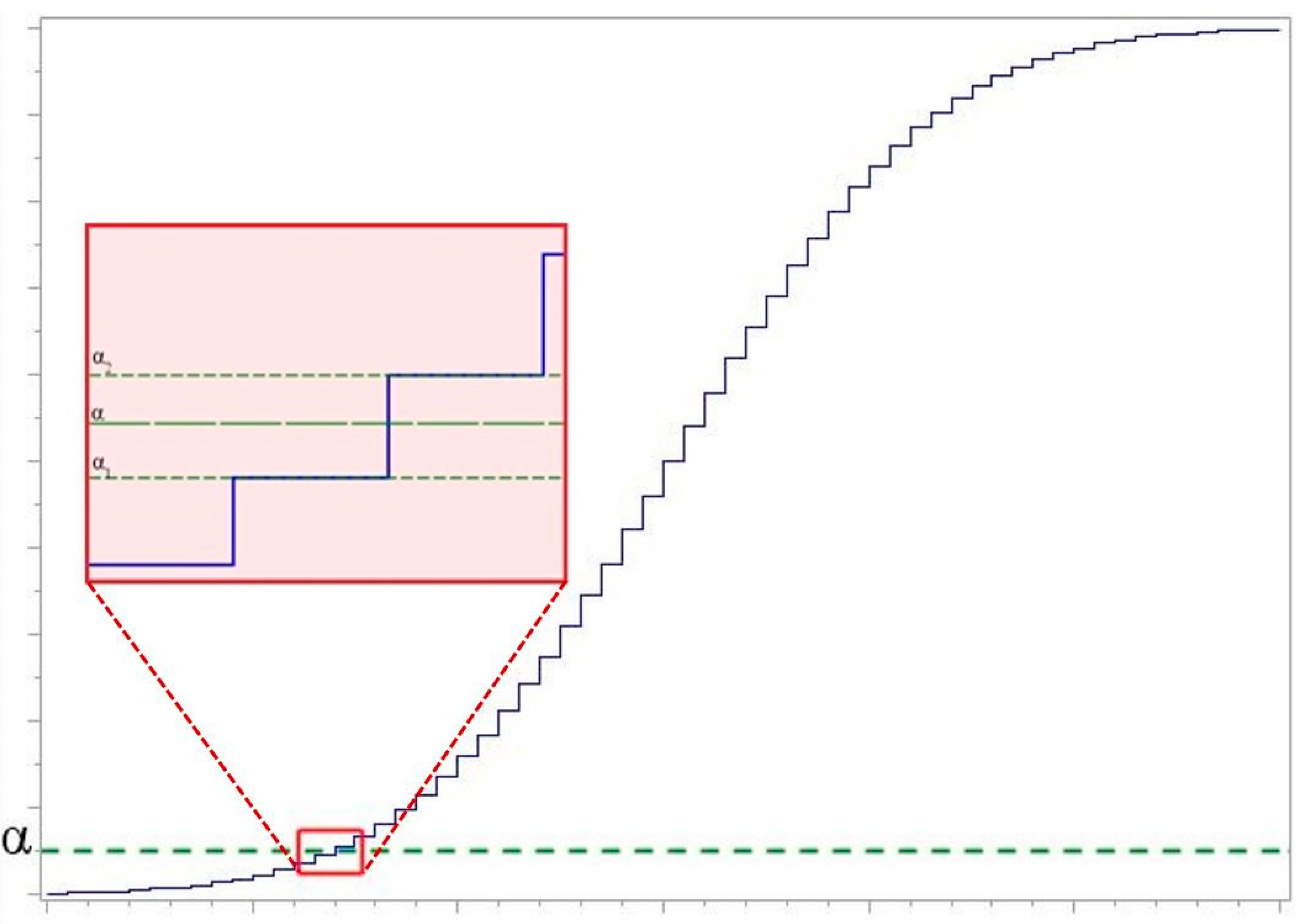
• Statistics of the compatibility hypothesis test criteria are calculated. If the obtain value of statistic is greater than the corresponding critical value ($\alpha =0.05$ is used), then hypothesis $H_0$ is rejected.
• Steps 1 and 2 are repeated for $k$ (in our experiments, $k=1,000,000$) times.
• The power of a test is calculated as $count/k$, where $count$ is the number of false hypotheses rejections.

4. Statistical Distributions

The simulation study considers fifteen statistical distributions for which the performance of the presented normality tests are assessed. Statistical distributions are grouped into three groups: symmetric, asymmetric, and modified normal distributions. A description of these distribution groups is presented in the following.

4.1. Symmetric Distributions

Symmetric distributions considered in this research are [20]:

• three cases of the $Beta\left(a, b\right)$ distribution$—Beta\left(0.5;0.5\right), Beta\left(1;1\right),$and $Beta\left(2;2\right)$, where $a$ and $b$ are the shape parameters;
• three cases of the $Cauchy\left(t, s\right)$ distribution—$Cauchy\left(0;0.5\right), Cauchy\left(0;1\right)$, and $Cauchy\left(0;2\right)$, where$t$ and$s$ are the location and scale parameters;
• one case of the $Laplace\left(t, s\right)$distribution$—Laplace\left(0;1\right)$, where $t$ and$s$ are the location and scale parameters;
• one case of the $Logistic\left(t, s\right)$ distribution$—Logistic\left(2;2\right)$, where $t$ and$s$ are the location and scale parameters;
• four cases of the $t-Student\left(\nu \right)$ distribution$—t\left(1\right), t\left(2\right), t\left(4\right),$ and $t\left(10\right)$, where $\nu$ is the number of degrees of freedom;
• five cases of the $Tukey\left(\lambda \right)$ distribution$—Tukey\left(0.14\right), Tukey\left(0.5\right), Tukey\left(2\right), Tukey\left(5\right),$ and $Tukey\left(10\right)$, where $\lambda$ is the shape parameter; and
• one case of the standard normal $N\left(0;1\right)$ distribution.

4.2. Asymmetric Distributions

Asymmetric distributions considered in this research are [20]:

• four cases of the $Beta\left(a,b\right)$ distribution$—Beta\left(2;1\right),Beta\left(2;5\right),Beta\left(4;0.5\right),$ and $Beta\left(5;1\right)$;
• four cases of the $Chi$-$squared\left(\nu \right)$ distribution$—{\chi }^2\left(1\right),{\chi }^2\left(2\right),{\chi }^2\left(4\right)$, and${\chi }^2\left(10\right)$, where $\nu$ is the number of degrees of freedom;
• six cases of the $Gamma\left(a,b\right)$ distribution—$Gamma\left(2;2\right),Gamma\left(3;2\right),Gamma\left(5;1\right),Gamma\left(9;1\right),Gamma\left(15;1\right)$, and $Gamma\left(100;1\right)$, where $a$ and $b$ are the shape and scale parameters;
• one case of the $Gumbel\left(t,s\right)$ distribution$—Gumbel\left(1;2\right)$, where $t$ and$s$ are the location and scale parameters;
• one case of the $Lognormal\left(t,s\right)$ distribution$—LN\left(0;1\right)$, where $t$ and$s$ are the location and scale parameters; and
• four cases of the $Weibull\left(a,b\right)$ distribution$—Weibull\left(0.5;1\right),Weibull\left(1;2\right),Weibull\left(2;3.4\right),$ and $Weibull\left(3;4\right)$, where $a$ and $b$ are the shape and scale parameters.

4.3. Modified Normal Distributions

Modified normal distributions considered in this research are [20]:

• six cases of the standard normal distribution truncated at $a$ and $b$ $Trunc\left(a;b\right)—Trunc\left(-1;1\right),Trunc\left(-2;2\right),Trunc\left(-3;3\right),Trunc\left(-2;1\right),Trunc\left(-3;1\right),$and $Trunc\left(-3;2\right),$ which are referred to as NORMAL1;
• nine cases of a location-contaminated standard normal distribution, hereon termed $LoConN\left(p;a\right)—LoConN\left(0.3;1\right),LoConN\left(0.4;1\right),LoConN\left(0.5;1\right),LoConN\left(0.3;3\right),$$LoConN\left(0.4;3\right),LoConN\left(0.5;3\right),LoConN\left(0.3;5\right),LoConN\left(0.4;5\right),$and $LoConN\left(0.5;5\right)$, which are referred to as NORMAL2;
• nine cases of a scale-contaminated standard normal distribution, hereon termed $ScConN\left(p;b\right)—ScConN\left(0.05;0.25\right),ScConN\left(0.10;0.25\right),ScConN\left(0.20;0.25\right),$$ScConN\left(0.05;2\right),ScConN\left(0.10;2\right),ScConN\left(0.20;2\right),ScConN\left(0.05;4\right),ScConN\left(0.10;4\right),$and $ScConN\left(0.20;4\right)$, which are referred to as NORMAL3; and
• twelve cases of a mixture of normal distributions, hereon termed $MixN\left(p;a;b\right)—MixN\left(0.3;1;0.25\right),MixN\left(0.4;1;0.25\right),MixN\left(0.5;1;0.25\right),MixN\left(0.3;3;0.25\right),$$MixN\left(0.4;3;0.25\right),MixN\left(0.5;3;0.25\right),MixN\left(0.3;1;4\right),MixN\left(0.4;1;4\right),MixN\left(0.5;1;4\right),$$MixN\left(0.3;3;4\right),MixN\left(0.4;3;4\right),$and $MixN\left(0.5;3;4\right)$, which are referred to as NORMAL4.

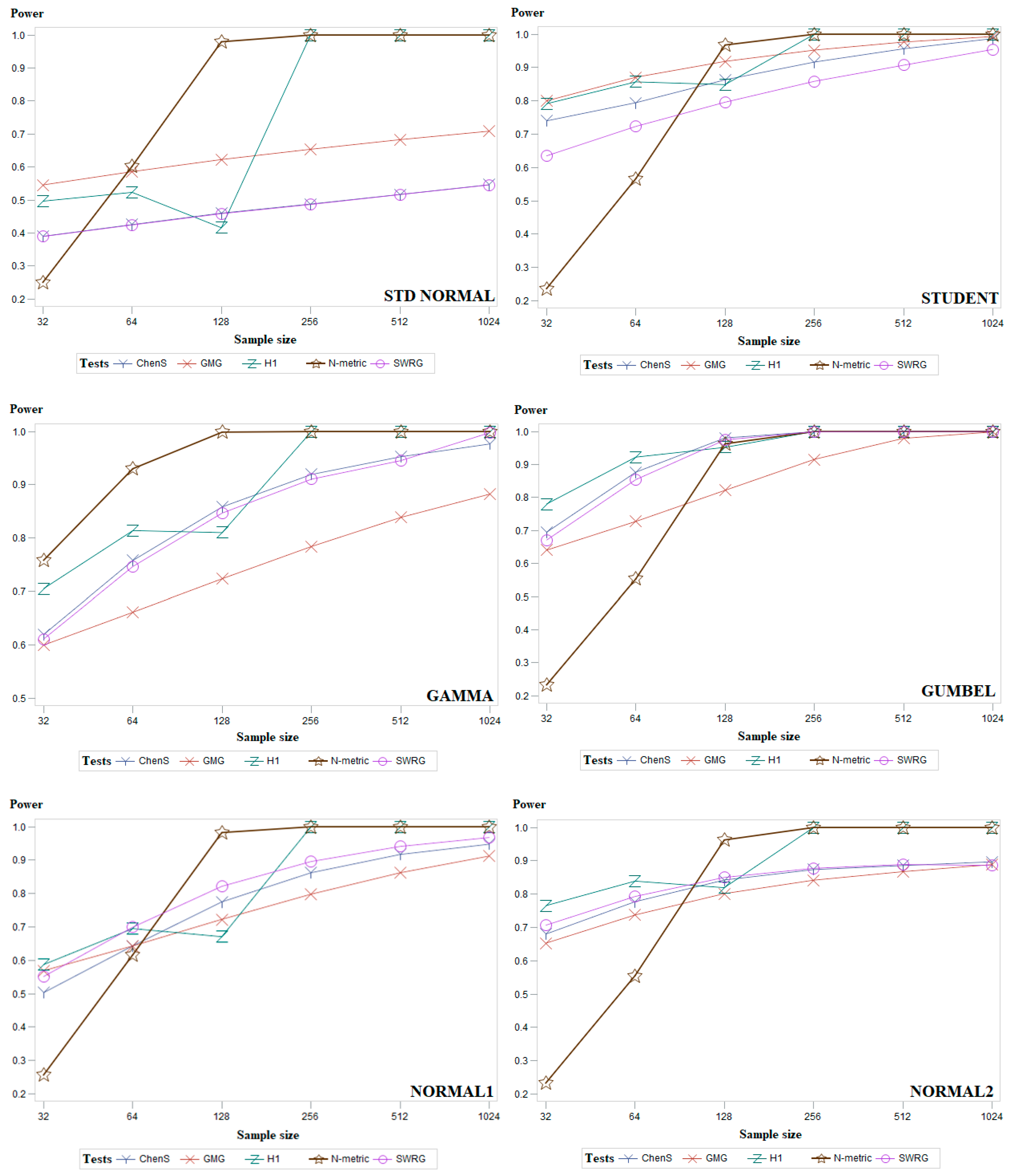
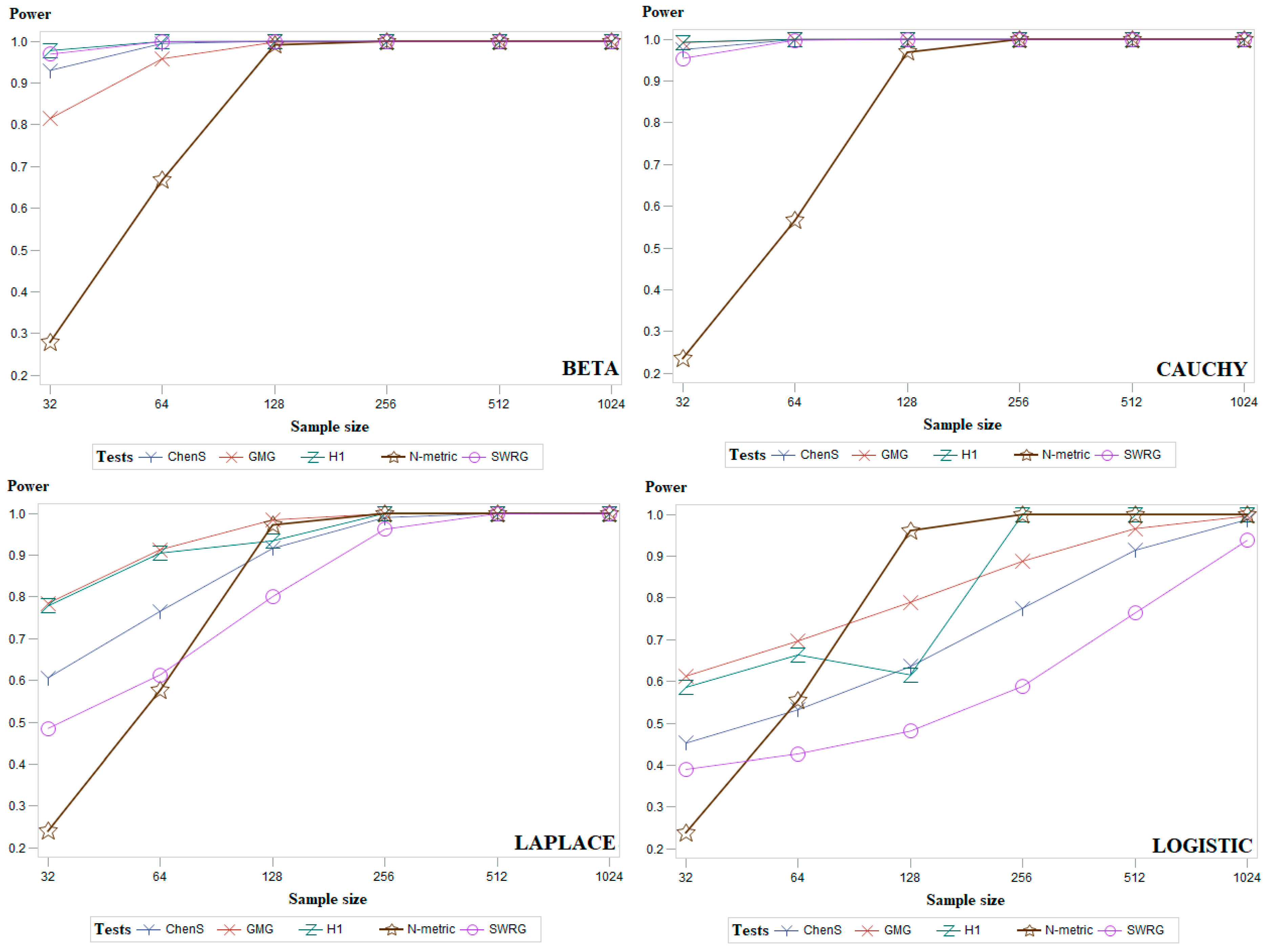
5. Simulation Study and Discussion

This section provides a comprehensive modeling study that is designed to evaluate the power of selected normality tests. This modeling study takes into account the effects of sample size, the level of significance ($\alpha =0.05$) chosen, and the alternative type of distribution (Beta, Cauchy, Laplace, Logistic, Student, Chi-Square, Gamma, Gumbel, Lognormal, Weibull, and modified standard normal). The study was performed by applying 40 normality tests (including our proposed normality test) for the generated 1,000,000 standardized samples of size 32, 64, 128, 256, 512, and 1024.

The best set of parameters $\left(a, b, c\right)$ was selected experimentally: the value of $a$ was examined from 0.001 to 0.99 by step 0.01, the value of $b$ was examined from 0.01 to 10 by step 0.01, and the value of $c$ was examined from 0.5 to 50 by step 0.25. The N-metric test gave the most powerful results with the parameters: $a=0.95, b=0.25, c=1$. In those cases, a test has several modifications, we present results only for the best variant. The

Table 1. Average empirical power obtained for a group of symmetric distributions.

		Sample Size
		32	64	128	256	512	1024
Tests	AD	0.714	0.799	0.863	0.909	0.939	0.955
	BCMR	0.718	0.809	0.875	0.920	0.947	0.947
	BHS	0.431	0.551	0.663	0.752	0.818	0.868
	BHSBS	0.680	0.778	0.783	0.903	0.938	0.959
	BM2	0.726	0.835	0.905	0.945	0.965	0.974
	BS	0.717	0.810	0.877	0.920	0.947	0.961
	CC2	0.712	0.805	0.873	0.920	0.949	0.936
	CHI2	0.663	0.778	0.842	0.884	0.941	0.945
	CVM	0.591	0.733	0.805	0.855	0.919	0.949
	ChenS	0.729	0.806	0.871	0.915	0.943	0.960
	Coin	0.735	0.830	0.891	0.930	0.952	0.963
	DA	0.266	0.295	0.314	0.319	0.315	0.311
	DAP	0.723	0.820	0.883	0.924	0.948	0.962
	DH	0.709	0.805	0.877	0.925	0.950	0.963
	DLDMZEPD	0.730	0.826	0.889	0.929	0.952	0.963
	EP	0.706	0.828	0.974	0.910	0.946	0.959
	Filli	0.712	0.805	0.875	0.922	0.949	0.962
	GG	0.658	0.760	0.850	0.915	0.949	0.962
	GLB	0.712	0.798	0.863	0.909	0.943	0.918
	GMG	0.787	0.862	0.914	0.946	0.965	0.975
	H1	0.799	0.862	0.852	0.999	0.999	0.999
	JB	0.643	0.762	0.856	0.918	0.949	0.963
	KS	0.585	0.723	0.789	0.836	0.905	0.939
	Lillie	0.669	0.758	0.828	0.883	0.921	0.947
	MI	0.632	0.676	0.705	0.724	0.736	0.745
	N-metric	0.245	0.585	0.971	0.999	0.999	0.999
	SF	0.715	0.807	0.876	0.923	0.949	0.962
	SW	0.718	0.808	0.874	0.919	0.946	0.962
	SWRG	0.694	0.775	0.834	0.882	0.916	0.946
	ZQstar	0.513	0.576	0.630	0.669	0.697	0.718
	ZW2	0.715	0.806	0.869	0.912	0.939	0.957

,

Table 2. Average empirical power obtained for a group of asymmetric distributions.

		Sample Size
		32	64	128	256	512	1024
Tests	AD	0.729	0.835	0.908	0.949	0.969	0.984
	BCMR	0.749	0.856	0.924	0.971	0.995	0.991
	BHS	0.529	0.664	0.769	0.855	0.915	0.950
	BHSBS	0.538	0.652	0.747	0.914	0.902	0.944
	BM2	0.737	0.859	0.931	0.965	0.981	0.993
	BS	0.506	0.588	0.665	0.738	0.805	0.859
	CC2	0.579	0.682	0.777	0.853	0.938	0.956
	CHI2	0.645	0.799	0.881	0.934	0.965	0.980
	CVM	0.594	0.755	0.836	0.887	0.935	0.957
	ChenS	0.756	0.862	0.928	0.961	0.978	0.991
	Coin	0.480	0.556	0.630	0.700	0.769	0.916
	DA	0.237	0.223	0.209	0.198	0.191	0.192
	DAP	0.705	0.826	0.910	0.955	0.977	0.990
	DH	0.724	0.845	0.921	0.957	0.977	0.991
	DLDMXAPD	0.726	0.843	0.918	0.955	0.975	0.989
	EP	0.753	0.846	0.913	0.967	0.975	0.993
	Filli	0.732	0.842	0.915	0.953	0.974	0.991
	GG	0.672	0.805	0.898	0.949	0.973	0.988
	GLB	0.725	0.831	0.905	0.987	0.970	0.984
	GMG	0.683	0.751	0.809	0.859	0.901	0.932
	H1	0.816	0.896	0.896	0.999	0.999	0.999
	JB	0.662	0.808	0.904	0.953	0.975	0.989
	KS	0.582	0.736	0.810	0.863	0.921	0.945
	Lillie	0.671	0.786	0.872	0.929	0.959	0.976
	MI	0.644	0.731	0.798	0.843	0.872	0.913
	N-metric	0.464	0.761	0.990	0.999	0.999	0.999
	SF	0.736	0.846	0.918	0.955	0.975	0.989
	SW	0.753	0.859	0.925	0.959	0.977	0.991
	SWRG	0.758	0.861	0.927	0.960	0.977	0.999
	ZQstar	0.570	0.639	0.693	0.732	0.761	0.748
	ZW2	0.764	0.870	0.932	0.962	0.980	0.997

and

Table 3. Average empirical power obtained for a group of modified normal distributions.

		Sample Size
		32	64	128	256	512	1024
Tests	AD	0.662	0.756	0.825	0.872	0.905	0.931
	BCMR	0.652	0.756	0.831	0.880	0.913	0.935
	BHS	0.463	0.585	0.676	0.744	0.796	0.834
	BHSBS	0.568	0.701	0.787	0.847	0.890	0.918
	BM2	0.641	0.770	0.854	0.904	0.934	0.953
	BS	0.587	0.688	0.770	0.833	0.881	0.916
	CC2	0.576	0.675	0.763	0.833	0.887	0.923
	CHI2	0.566	0.728	0.808	0.866	0.914	0.939
	CVM	0.557	0.708	0.779	0.833	0.897	0.930
	ChenS	0.656	0.759	0.833	0.882	0.915	0.937
	Coin	0.579	0.691	0.781	0.846	0.889	0.918
	DA	0.314	0.342	0.367	0.388	0.405	0.418
	DAP	0.617	0.733	0.818	0.872	0.906	0.930
	DH	0.617	0.727	0.815	0.872	0.907	0.930
	DLDMXAPD	0.651	0.754	0.831	0.879	0.912	0.935
	EP	0.640	0.748	0.819	0.865	0.906	0.931
	Filli	0.637	0.743	0.823	0.877	0.911	0.933
	GG	0.529	0.657	0.775	0.860	0.906	0.932
	GLB	0.659	0.755	0.823	0.870	0.903	0.930
	GMG	0.688	0.771	0.836	0.883	0.917	0.942
	H1	0.743	0.816	0.799	0.999	0.999	0.999
	JB	0.515	0.662	0.783	0.861	0.904	0.930
	KS	0.564	0.710	0.772	0.825	0.893	0.924
	Lillie	0.626	0.724	0.796	0.850	0.889	0.917
	MI	0.494	0.536	0.563	0.578	0.585	0.590
	N-metric	0.243	0.582	0.972	0.999	0.999	0.999
	SF	0.642	0.747	0.826	0.879	0.912	0.934
	SW	0.654	0.758	0.832	0.882	0.915	0.937
	SWRG	0.643	0.746	0.818	0.864	0.901	0.931
	ZQstar	0.394	0.423	0.450	0.472	0.487	0.498
	ZW2	0.640	0.749	0.826	0.876	0.907	0.931

present average power obtained for the symmetric, asymmetric, and modified normal distribution sets, for samples sizes of 32, 64, 128, 256, 512, and 1024. By comparing Table 1, Table 2 and Table 3, it can be seen that the most powerful test for small samples was Hosking1 (H1), the most powerful test for large sample sizes was our presented test (N-metric). According to Table 1, Table 2 and Table 3, it is observed that for large sample sizes, most tests’ power is approaching 1 except for the D’Agostino (DA) test, the power of which is significantly lower.

An additional study was conducted to determine the exact minimal sample size at which the N-metric test (statistic (34) with kernel function (35)) is the most powerful for groups of symmetric, asymmetric, and modified normal distributions. Hosking1 and N-metric tests were applied for data sets of sizes: 80, 90, 100, 105, 110, and 115. The obtained results showed that the N-metric test was the most powerful for sample size $\ge 112$ for the symmetric distributions, for sample size $\ge 118$ for the asymmetric distributions, and for sample size $\ge 88$ for a group of modified normal distributions (see in

Table 4. The minimal sample size at which the N-metric test is most powerful.

Nr.	Distribution	Groups of Distributions	$\mathbf{Minimal}\mathbf{Sample}\mathbf{Size}\left(\mathit{n}\right)$
1.	Standard normal	Symmetric	46
2.	Beta	Symmetric	88
3.	Cauchy	Symmetric	257
4.	Laplace	Symmetric	117
5.	Logistic	Symmetric	71
6.	Student	Symmetric	96
7.	Beta	Asymmetric	108
8.	Chi-square	Asymmetric	123
9.	Gamma	Asymmetric	<32
10.	Gumbel	Asymmetric	125
11.	Lognormal	Asymmetric	255
12.	Weibull	Asymmetric	65
13.	Normal1	Modified normal	70
14.	Normal2	Modified normal	93
15.	Normal3	Modified normal	72
16.	Normal4	Modified normal	117

). The N-metric test is the most powerful for the Gamma distribution for sample size $\ge 32$. It has been observed that in the case of Cauchy and Lognormal distributions, the N-metric test is the most powerful when the sample size is $\ge 255$, which can be influenced by the long tail of these distributions.

To complement the results given in Table 1, Table 2 and Table 3, Figure 4 (and Figure A1, Figure A2 and Figure A3 in Appendix A) presents the average power results of the most powerful goodness-of-fit tests. Figure 4 presents two distributions from each group of symmetric (Standard normal and Student), asymmetric (Gamma and Gumbel), and modified normal (standard normal distribution truncated at $a$ and $b$ and location-contaminated standard normal distribution) distributions. Figures of all other distributions are given in Appendix A. In Figure 4, it can be seen that for the standard normal distribution, our proposed test (N-metric) is the most powerful when the sample size is 64 or larger. Figure 4 shows that our proposed test (N-metric) is the most powerful in the case of Gamma data distribution for all sample sizes examined. In general, it can be summarized that the power of the Chen–Shapiro (ChenS), Gel–Miao–Gastwirth (GMG), Hosking1 (H1), and Modified Shapiro–Wilk (SWRG) tests increases gradually with increasing sample size. The power of our proposed test (N-metric) increases abruptly when the sample size is 128 and its power value remains close to 1 for larger sample sizes.

6. Conclusions and Future Work

In this study, a comprehensive comparison of the power of popular normality tests was performed. Given the importance of this topic and the extensive development of normality tests, the proposed new normality test, the detailed test descriptions provided, and the power comparisons are relevant. Only univariate data were examined in this study of the power of normality tests (a study with multivariate data is planned for the future).

The study addresses the performance of 40 normality tests, for various sample sizes $n$ for a number of symmetric, asymmetric, and modified normal distributions. A new goodness-of-fit test has been proposed. Its results are compared with other tests.

Based on the obtained modeling results, it was determined that the most powerful tests for the groups of symmetric, asymmetric, and modified normal distributions were Hosking1 (for smaller sample sizes) and our proposed N-metric (for larger sample sizes) test. The power of the Hosking1 test (for smaller sample sizes) is 1.5 to 7.99 percent higher than the second (by power) test for the groups of symmetric, asymmetric, and modified normal distributions. The power of the N-metric test (for larger sample sizes) is 6.2 to 16.26 percent higher than the second (by power) test for the groups of symmetric, asymmetric, and modified normal distributions.

The N-metric test is recommended to be used for symmetric data sets of size $n\ge 112$, for asymmetric data sets of size $n\ge 118$, and for bell-shaped distributed data sets of size $n\ge 88$.

References

- Barnard, G.A.; Barnard, G.A. Introduction to Pearson (1900) on the Criterion That a Given System of Deviations from the Probable in the Case of a Correlated System of Variables is Such That it Can be Reasonably Supposed to Have Arisen from Random Sampling; Springer Series in Statistics Breakthroughs in Statistics; Springer: Cham, Switzerland, 1992; pp. 1–10. [Google Scholar]
- Kolmogorov, A. Sulla determinazione empirica di una legge di distribuzione. Inst. Ital. Attuari Giorn. 1933, 4, 83–91. [Google Scholar]
- Adefisoye, J.; Golam Kibria, B.; George, F. Performances of several univariate tests of normality: An empirical study. J. Biom. Biostat. 2016, 7, 1–8. [Google Scholar]
- Anderson, T.W.; Darling, D.A. Asymptotic theory of certain “goodness-of-fit” criteria based on stochastic processes. Ann. Math. Stat. 1952, 23, 193–212. [Google Scholar] [CrossRef]
- Hosking, J.R.M.; Wallis, J.R. Some statistics useful in regional frequency analysis. Water Resour. Res. 1993, 29, 271–281. [Google Scholar] [CrossRef]
- Cabana, A.; Cabana, E.M. Goodness-of-Fit and Comparison Tests of the Kolmogorov-Smirnov Type for Bivariate Populations. Ann. Stat. 1994, 22, 1447–1459. [Google Scholar] [CrossRef]
- Chen, L.; Shapiro, S.S. An Alternative Test for Normality Based on Normalized Spacings. J. Stat. Comput. Simul. 1995, 53, 269–288. [Google Scholar] [CrossRef]
- Rahman, M.M.; Govindarajulu, Z. A modification of the test of Shapiro and Wilk for normality. J. Appl. Stat. 1997, 24, 219–236. [Google Scholar] [CrossRef]
- Ray, W.D.; Shenton, L.R.; Bowman, K.O. Maximum Likelihood Estimation in Small Samples. J. R. Stat. Soc. Ser. A 1978, 141, 268. [Google Scholar] [CrossRef]
- Zhang, P. Omnibus test of normality using the Q statistic. J. Appl. Stat. 1999, 26, 519–528. [Google Scholar] [CrossRef]
- Barrio, E.; Cuesta-Albertos, J.A.; Matrán, C.; Rodríguez-Rodríguez, J.M. Tests of goodness of fit based on the L2-Wasserstein distance. Ann. Stat. 1999, 27, 1230–1239. [Google Scholar]
- Glen, A.G.; Leemis, L.M.; Barr, D.R. Order statistics in goodness-of-fit testing. IEEE Trans. Reliab. 2001, 50, 209–213. [Google Scholar] [CrossRef]
- Bonett, D.G.; Seier, E. A test of normality with high uniform power. Comput. Stat. Data Anal. 2002, 40, 435–445. [Google Scholar] [CrossRef]
- Psaradakis, Z.; Vávra, M. Normality tests for dependent data: Large-sample and bootstrap approaches. Commun. Stat.-Simul. Comput. 2018, 49, 283–304. [Google Scholar] [CrossRef]
- Zhang, J.; Wu, Y. Likelihood-ratio tests for normality. Comput. Stat. Data Anal. 2005, 49, 709–721. [Google Scholar] [CrossRef]
- Gel, Y.R.; Miao, W.; Gastwirth, J.L. Robust directed tests of normality against heavy-tailed alternatives. Comput. Stat. Data Anal. 2007, 51, 2734–2746. [Google Scholar] [CrossRef]
- Coin, D. A goodness-of-fit test for normality based on polynomial regression. Comput. Stat. Data Anal. 2008, 52, 2185–2198. [Google Scholar] [CrossRef]
- Desgagné, A.; Lafaye de Micheaux, P. A powerful and interpretable alternative to the Jarque–Bera test of normality based on 2nd-power skewness and kurtosis, using the Rao’s score test on the APD family. J. Appl. Stat. 2017, 45, 2307–2327. [Google Scholar] [CrossRef]
- Steele, C.M. The Power of Categorical Goodness-Of-Fit Statistics. Ph.D. Thesis, Australian School of Environmental Studies, Warrandyte, Victoria, Australia, 2003. [Google Scholar]
- Romão, X.; Delgado, R.; Costa, A. An empirical power comparison of univariate goodness-of-fit tests for normality. J. Stat. Comput. Simul. 2010, 80, 545–591. [Google Scholar] [CrossRef]
- Choulakian, V.; Lockhart, R.; Stephens, M. Cramérvon Mises statistics for discrete distributions. Can. J. Stat. 1994, 22, 125–137. [Google Scholar] [CrossRef]
- Shapiro, S.S.; Wilk, M.B. An analysis of variance test for normality (complete samples). Biometrika 1965, 52, 591–611. [Google Scholar] [CrossRef]
- Lilliefors, H.W. On the Kolmogorov-Smirnov test for normality with mean and variance unknown. J. Am. Stat. Assoc. 1967, 62, 399–402. [Google Scholar] [CrossRef]
- Ahmad, F.; Khan, R.A. A power comparison of various normality tests. Pak. J. Stat. Oper. Res. 2015, 11, 331. [Google Scholar] [CrossRef]
- D’Agostino, R.B.; Pearson, E.S. Testing for departures from normality. I. Fuller empirical results for the distribution of b2 and √b1. Biometrika 1973, 60, 613–622. [Google Scholar]
- Filliben, J.J. The Probability Plot Correlation Coefficient Test for Normality. Technometrics 1975, 17, 111–117. [Google Scholar] [CrossRef]
- Martinez, J.; Iglewicz, B. A test for departure from normality based on a biweight estimator of scale. Biometrika 1981, 68, 331–333. [Google Scholar] [CrossRef]
- Epps, T.W.; Pulley, L.B. A test for normality based on the empirical characteristic function. Biometrika 1983, 70, 723–726. [Google Scholar] [CrossRef]
- Jarque, C.; Bera, A. Efficient tests for normality, homoscedasticity andserial independence of regression residuals. Econ. Lett. 1980, 6, 255–259. [Google Scholar] [CrossRef]
- Bakshaev, A. Goodness of fit and homogeneity tests on the basis of N-distances. J. Stat. Plan. Inference 2009, 139, 3750–3758. [Google Scholar] [CrossRef]
- Hill, T.; Lewicki, P. Statistics Methods and Applications; StatSoft: Tulsa, OK, USA, 2007. [Google Scholar]
- Kasiulevičius, V.; Denapienė, G. Statistikos taikymas mokslinių tyrimų analizėje. Gerontologija 2008, 9, 176–180. [Google Scholar]
- Damianou, C.; Kemp, A.W. New goodness of statistics for discrete and continuous data. Am. J. Math. Manag. Sci. 1990, 10, 275–307. [Google Scholar]