Wall Shear Stress Topological Skeleton Analysis in Cardiovascular Flows: Methods and Applications

Abstract

A marked interest has recently emerged regarding the analysis of the wall shear stress (WSS) vector field topological skeleton in cardiovascular flows. Based on dynamical system theory, the WSS topological skeleton is composed of fixed points, i.e., focal points where WSS locally vanishes, and unstable/stable manifolds, consisting of contraction/expansion regions linking fixed points. Such an interest arises from its ability to reflect the presence of near-wall hemodynamic features associated with the onset and progression of vascular diseases. Over the years, Lagrangian-based and Eulerian-based post-processing techniques have been proposed aiming at identifying the topological skeleton features of the WSS. Here, the theoretical and methodological bases supporting the Lagrangian- and Eulerian-based methods currently used in the literature are reported and discussed, highlighting their application to cardiovascular flows. The final aim is to promote the use of WSS topological skeleton analysis in hemodynamic applications and to encourage its application in future mechanobiology studies in order to increase the chance of elucidating the mechanistic links between blood flow disturbances, vascular disease, and clinical observations.

1. Introduction

Recent advances in medical imaging, modeling, and computational fluid dynamics (CFD) have allowed the modeling of local hemodynamics in realistic, personalized cardiovascular models, fostering understanding of the association between local hemodynamics and the initiation and progression of vascular disease, and in a wider perspective, contributing to the translation of computational methods in real-world clinical settings to complement clinical information.

It has long been recognized that hemodynamic factors regulate several aspects of vascular pathophysiology [1,2]. Wall shear stress (WSS), the frictional force per unit area exerted by streaming blood on the endothelium, has been identified as a major biomechanical factor involved in vascular homeostasis. In fact, WSS is sensed through several vascular mechanosensors and biochemical machineries that regulate the expression of genes coding for extra- and intra-cellular proteins, playing a relevant role in the development, growth, remodeling, and maintenance of the vascular system [3,4]. In this scenario, a multitude of WSS-based descriptors of the near-wall hemodynamics has been proposed over the years to provide potential indicators of flow disturbances associated with aggravating biological events. In particular, regions at the luminal surface presenting with low [5] and oscillatory [6] WSS have been identified as localizing factors of vascular disease [3,6]. However, the complex hemodynamic milieu the endothelium is exposed to can be only partially characterized by low and oscillatory WSS [7,8], as confirmed by a large body of literature reporting poor-to-moderate (and sometimes, contradictory) associations between low and oscillatory WSS with respect to vascular disease, e.g., [7,8,9,10,11,12,13]. This indicates a limited current understanding of the mechanistic link between WSS and vascular disease that hampers the use of WSS not only as a biomarker of vascular disease but also as a predictor of its progression within a clinical context [14].

Stimulated by the need to improve the understanding of the link between altered hemodynamics and clinical observations, the topological skeleton of the WSS vector field at the luminal surface of an artery is receiving increasing interest [15,16,17,18,19,20]. Based on dynamical system theory, the WSS topological skeleton is composed of a collection of fixed points, i.e., focal points where WSS locally vanishes, and unstable/stable manifolds, consisting of contraction/expansion regions linking fixed points. Such an interest arises from the ability of WSS topological skeleton features to reflect cardiovascular flow features like flow stagnation, separation and recirculation that are known to be promoting factors for vascular disease [2,17]. Very recent studies have demonstrated that the WSS topological skeleton governs the near-wall biochemical transport in arteries [15,16,18,21], which plays a fundamental role in, e.g., the initiation of atherosclerosis and thrombogenesis [22,23]. In addition, evidence of a direct association between WSS topological skeleton features and markers of vascular diseases from real-world clinical data have recently emerged [20,24].

In the present study, we report and discuss the theoretical background of Lagrangian- and Eulerian-based methods currently applied to the analysis of the WSS topological skeleton. Based on the recent promising findings highlighting a link between WSS topological skeleton features and markers of vascular disease [17,18,19,20,21,24], the aim of this study is to encourage the application of WSS topological skeleton analysis to cardiovascular flows as an ad hoc instrument that is potentially able to further elucidate the mechanistic link between WSS and vascular pathophysiology.

2. Topological Skeleton of a Vector Field

Topological features of a vector field have been largely studied in the context of dynamical systems theory. A dynamical system is defined as a set of n differential equations:

$$\begin{gathered} \dot{\mathit{x}}\left(t\right)=\mathit{u}\left(\mathit{x},t\right); \\ \mathit{x}\left(t_0\right)={\mathit{x}}_{\mathbf{0}}, \end{gathered}$$

(1)

where $t \in {ℝ}^{+}$ is the time, ${\mathit{x}}_{\mathbf{0}}\in {ℝ}^{\mathit{n}}$ the initial position at time point $t_0$, i.e., ${\mathit{x}}_{\mathbf{0}}=\mathit{x}\left(t_0\right)$, and $\mathit{u}\left(\mathit{x},t\right)$ the velocity field. Given the initial condition ${\mathit{x}}_{\mathbf{0}}\in {ℝ}^{\mathit{n}}$, a unique solution of Equation (1) exists, called trajectory, given by:

$$\mathit{x}\left(t\right)=\mathit{x}\left(t_0\right)+{{\displaystyle \int }}_{t_0}^t\mathit{u}\left(\mathit{x}\left(s\right),s\right) ds.$$

(2)

Associated with the dynamical system defined in Equation (1), the so-called flow map can be defined as follows:

$${\mathsf{\Phi }}_{t_0}^t : {\mathit{x}}_{\mathbf{0}} \to \mathit{x}\left(t\right),$$

(3)

providing the expression of all the system trajectories at time $t$. In general, the topological skeleton of the vector field $\mathit{u}$is recognized to provide the organizing structures of the system itself.

In steady-state conditions (i.e., when vector field $\mathit{u}\left(\mathit{x},t\right)$ in Equation (1) does not explicitly depend on time), the topological skeleton of a vector field consists of a collection of fixed points (Figure 1A) and the associated stable and unstable manifolds connecting them (Figure 1B). A fixed point (or critical point) is a point ${\mathit{x}}_{fp}\in {ℝ}^{\mathit{n}}$ where the vector field locally vanishes. The nature of fixed points can be stable or unstable. A stable fixed point is characterized by a sink configuration, and it attracts the nearby trajectories, while an unstable fixed point is characterized by a source configuration, and it repels the nearby trajectories (Figure 1A).

A fixed point can be classified as a saddle point, node, or focus (Figure 1A): (1) a saddle point is a point attracting and repelling nearby trajectories along different directions (i.e., where the streamlines of the vector field intersect themselves); (2) a stable/unstable node is characterized by converging/diverging streamlines; (3) a focus is characterized by spiraling trajectories, and it can be attracting or repelling.

Technically, the exact location of fixed points in a domain of interest can be identified by computing the Poincaré index [25], a topological invariant index quantifying how many times a vector field rotates in the neighborhood of a point. For the sake of simplicity, we consider the dynamical system in Equation (1) under steady-state conditions and lying in a 2D space, i.e., $\mathit{u}\left(\mathit{x}\right)=\left(X\left(\mathit{x}\right),Y\left(\mathit{x}\right)\right)$, with $\mathit{x}\in {ℝ}^2$. An explanatory example of how to calculate the Poincaré index can then be provided. Let ${\mathit{x}}_{fp}\in {ℝ}^2$ be an isolated fixed point of $\mathit{u}$ with a neighborhood N such that there are no other fixed points in N than${\mathit{x}}_{fp}$, and let γ be a closed curve inscribing N. Then, the Poincaré index $ℐ\left(\gamma ,\mathit{u}\right)$ of the curve γ relative to $\mathit{u}$ is the number of the positive field rotations while traveling along γ in a positive direction:

$$ℐ\left(\gamma ,\mathit{u}\right)=\frac{1}{2 \pi } {{\displaystyle \int }}_{\mathsf{\Gamma }}^{}d\theta =\frac{1}{2 \pi } {{\displaystyle \int }}_{\mathsf{\Gamma }}^{}d arctan\left(\frac{Y}{X}\right),$$

(4)

where $\theta$ is the vector field rotation angle. The Poincaré index is equal to −1 at saddle point locations (Figure 1A), 1 at node or focus locations (Figure 1A), and 0 otherwise. The algorithm for computing the Poincaré index for a 3D vector field defined on unstructured triangle meshes is extensively described elsewhere [19].

The Poincaré index allows identifying fixed point locations, but it does not provide information about the fixed points nature. Therefore, a criterion to distinguish between a node or a focus and between the attractive or repelling nature of a fixed point is needed. In light of this, the vector field $\mathit{u}$ around the fixed point ${\mathit{x}}_{fp}$ can be expressed by linearization as:

$$\mathit{u}\left(\mathit{x}\right)=\mathit{u}\left({\mathit{x}}_{fp}\right)+J\left({\mathit{x}}_{fp}\right)\left(\mathit{x}-{\mathit{x}}_{fp}\right),$$

(5)

where J is the Jacobian matrix of $\mathit{u}$. The classification of fixed points can be thus performed by computing the eigenvalues of the Jacobian matrix J, as summarized in

Table 1. Classification of fixed points based on the eigenvalues of the Jacobian matrix.

λ	Fixed Point
${\lambda }_1<0<{\lambda }_2$	Saddle point
${\lambda }_1,{\lambda }_2>0$	Unstable node
${\lambda }_1,{\lambda }_2<0$	Stable node
${\lambda }_{1,2}=\alpha \pm \beta i$	Unstable focus
${\lambda }_{1,2}=-\alpha \pm \beta i$	Stable focus

. In detail, two real eigenvalues with different signs identify a saddle point. Two real eigenvalues with the same sign identify nodes characterized as attracting or repelling (i.e., stable or unstable, respectively) according to their sign (negative or positive, respectively). Complex conjugate eigenvalues identify a stable or unstable focus according to the sign of the real part (negative or positive, respectively).

The stable and unstable manifolds (or critical lines) associated with a fixed point ${\mathit{x}}_{fp}$ are composed of all initial conditions ${\mathit{x}}_{\mathbf{0}}\in {ℝ}^{\mathit{n}}$ such that the trajectories initiated at these points ${\mathit{x}}_{\mathbf{0}}$ approach the fixed point ${\mathit{x}}_{fp}$ asymptotically. By construction, stable and unstable manifolds act as separatrices of the vector field, portioning regions of different behavior and dynamics. In detail, an unstable manifold attracts nearby trajectories, as opposed to the stable manifold, which repels nearby trajectories (Figure 1B). In mathematical terms, an unstable manifold ${\mathit{W}}^{\mathit{u}}$ associated with the generic fixed point ${\mathit{x}}_{fp}$is defined as follows:

$${\mathit{W}}^{\mathit{u}}\left({\mathit{x}}_{fp}\right)=\left\{{\mathit{x}}_{\mathbf{0}}\in {ℝ}^{\mathit{n}}:{\mathsf{\Phi }}_{t_0}^t\left({\mathit{x}}_{\mathbf{0}}\right)\to {\mathit{x}}_{fp}\mathrm{as}t\to +\infty \right\},$$

(6)

while a stable manifold ${\mathit{W}}^{\mathit{s}}$can be expressed as:

$${\mathit{W}}^{\mathit{s}}\left({\mathit{x}}_{fp}\right)=\left\{{\mathit{x}}_{\mathbf{0}}\in {ℝ}^{\mathit{n}}:{\mathsf{\Phi }}_{t_0}^t\left({\mathit{x}}_{\mathbf{0}}\right)\to {\mathit{x}}_{fp}\mathrm{as}t\to -\infty \right\}.$$

(7)

In general, two different perspectives have been proposed to identify manifolds of a vector field, namely the Lagrangian and Eulerian perspectives. The Lagrangian perspective considers individual particles, tracking their motion along their paths as they are advected by the flow field. By contrast, the Eulerian perspective considers the properties of the vector field under analysis at each fixed location in space and time. In the following sections, a brief theoretical background is reported for a better understanding of the theory supporting the Lagrangian and Eulerian approaches for the analysis of vector field topology, with particular emphasis on their application to cardiovascular flows.

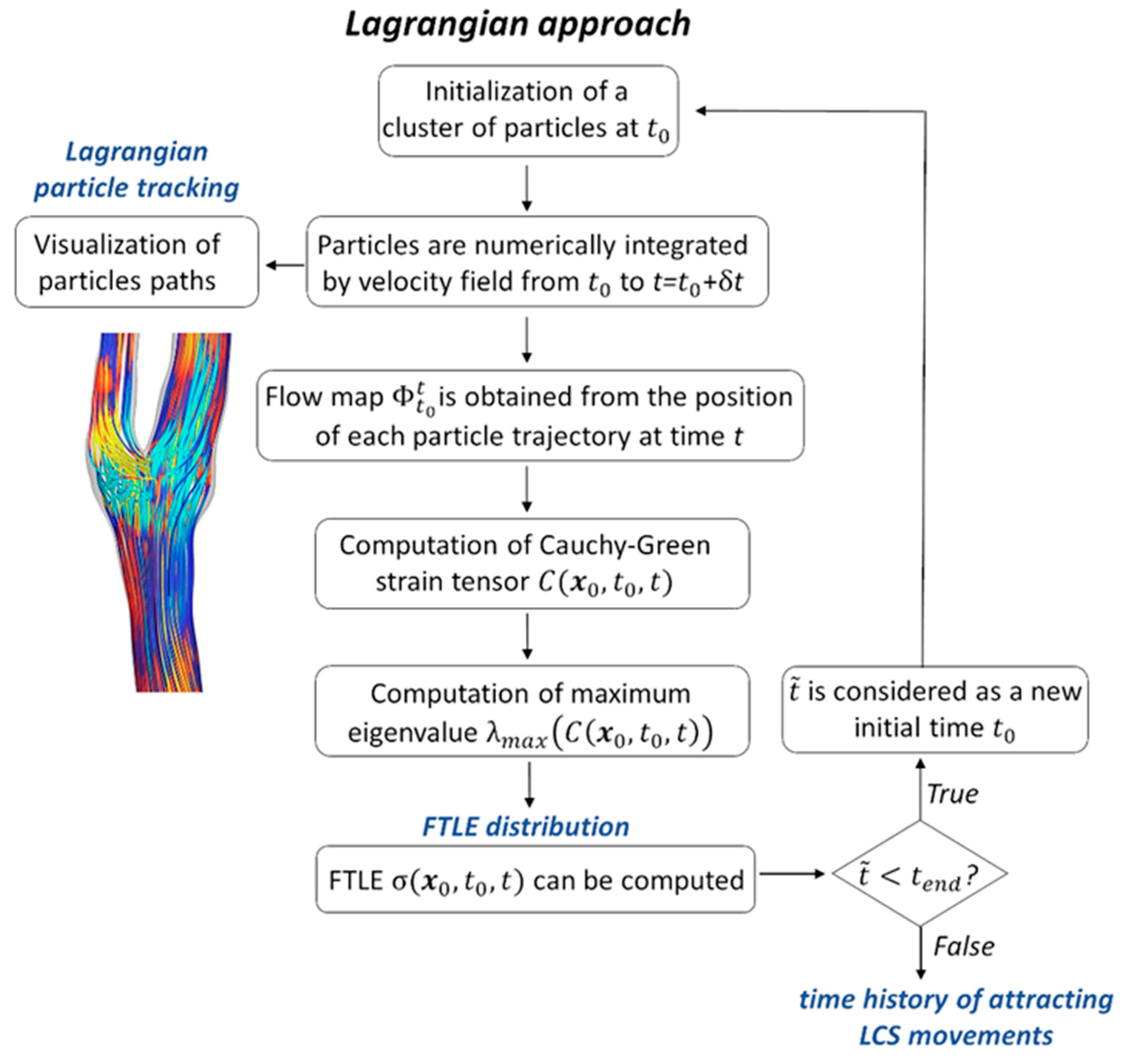
3. Lagrangian Approach

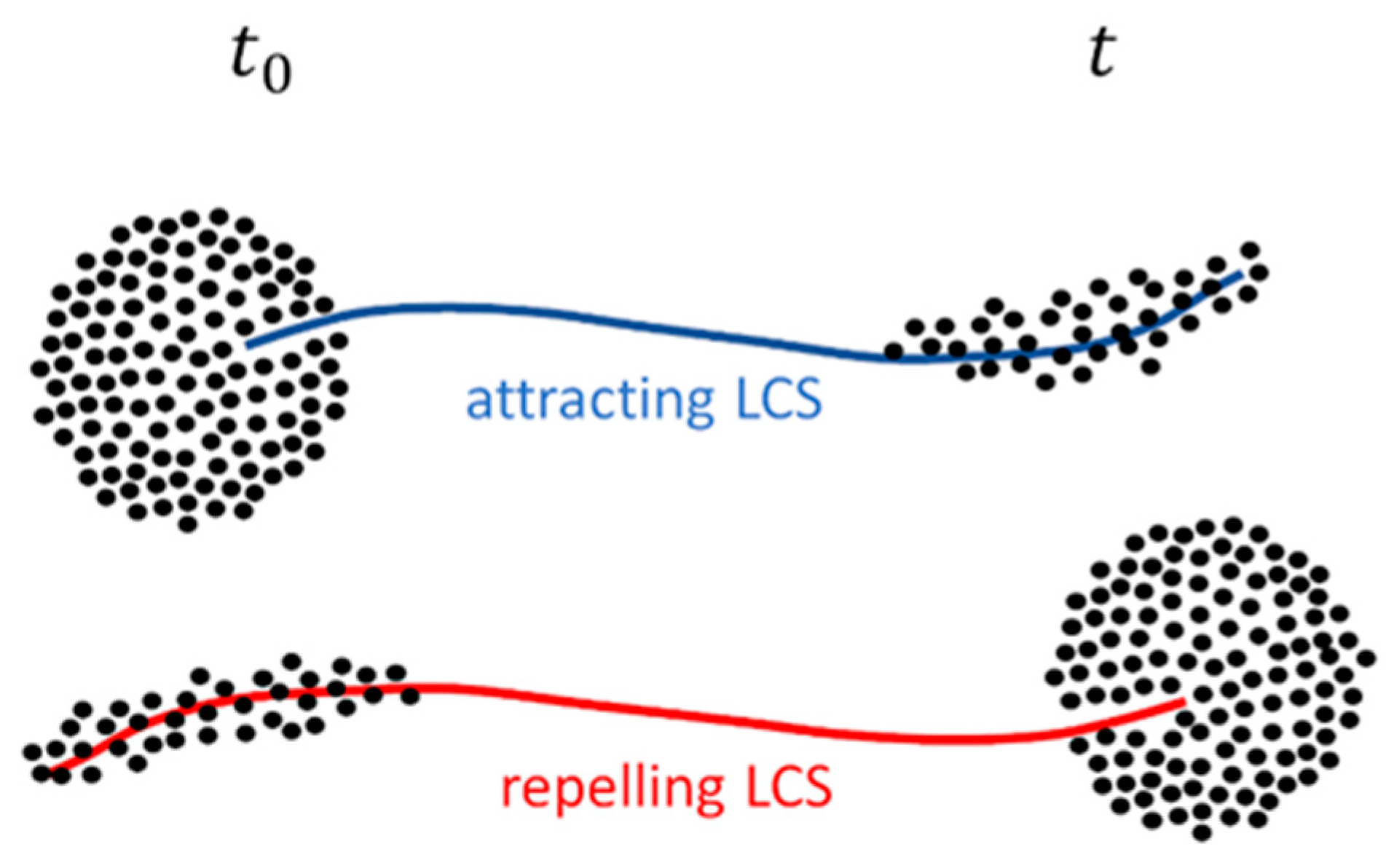
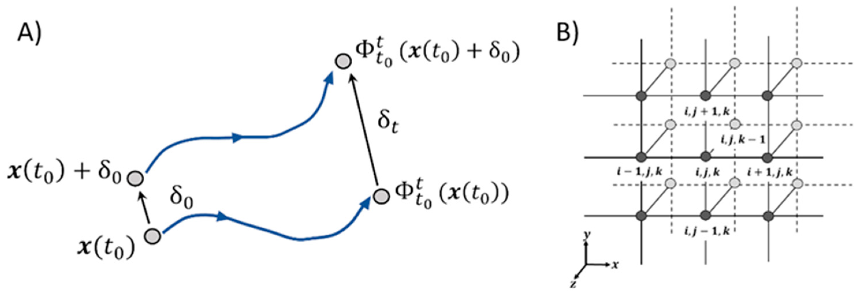
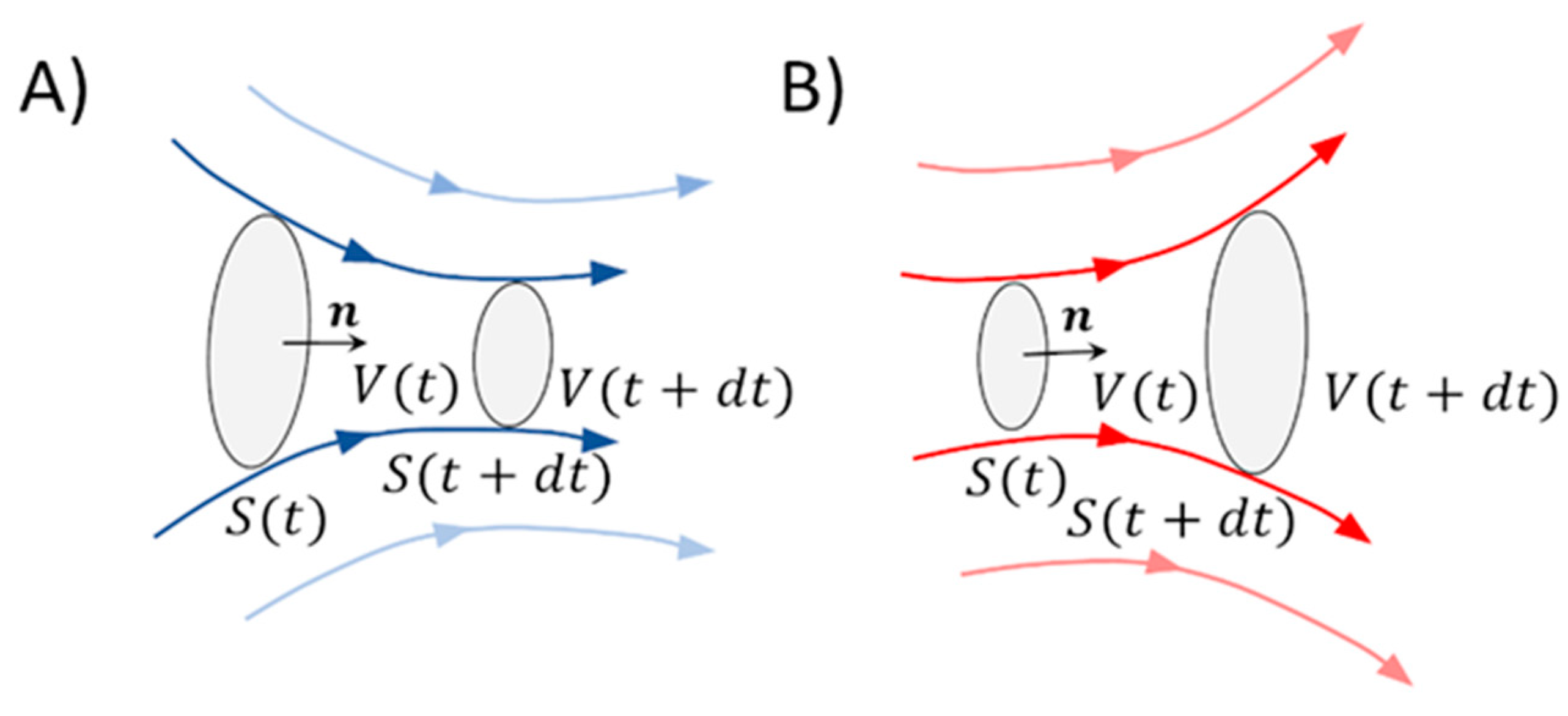
3.1. Lagrangian Coherent Structures

When the vector field $\mathit{u}\left(\mathit{x},t\right)$ in Equation (1) is time-dependent, solutions can be complex and chaotic, making the interpretation of the topological skeleton made of ${\mathit{W}}^{\mathit{u}},{\mathit{W}}^{\mathit{s}}$and ${\mathit{x}}_{fp}$ difficult. The need to robustly define intrinsic structures governing fluid/mass transport under unsteady-state conditions has led to the development of the concept of coherent structures (CS). Technically, CS are defined as emergent patterns, influencing the transport of tracers/mass in time-dependent flows [26]. In this context, Lagrangian Coherent Structures (LCS) are coherent structures identified by applying methods based on a Lagrangian approach. The theoretical bases of LCS lie in methods of nonlinear dynamics, chaos theory, and fluid dynamics.

From a mathematical perspective and in relation to fluid mechanics, LCS can be defined as material surfaces in the flow field that are dominant in attracting or repelling neighboring fluid elements over a defined time interval [27,28]. These material surfaces are able to localize where the flow field experiences the largest and the smallest stretching [29]. In detail, material surfaces in the flow field attracting trajectories more strongly than any other nearby material surface are referred to as attracting LCS. Oppositely, material surfaces repelling trajectories more strongly than any other nearby material surface are referred to as repelling LCS.

The detection and visualization of LCS is usually performed by applying two different Lagrangian-based approaches, namely (1) Lagrangian particle tracking and (2) the computation of the finite-time Lyapunov exponent (FTLE). Both approaches are based on particle path information derived from the post-processing of velocity data obtained by CFD simulation or by in vivo (e.g., phase contrast magnetic resonance imaging (MRI)) and in vitro (e.g., particle image velocimetry) measurements. The workflow of the Lagrangian-based approaches to visualize LCS is sketched in Figure 2.

The Lagrangian particle tracking is performed by seeding the domain of interest with tracer particles and by visualizing their motion (Figure 2). The aim of this approach is to reveal coherent features revealing how the flow under analysis is organized. From a mathematical perspective, the position of a tracer particle is governed by the differential equation reported in Equation (1). To obtain the position of such a particle at a desired time $t$, Equation (1) is numerically integrated from $t_0$ to $t$. The direct integration of tracer particles allows for an in-depth understanding of how tracers are transported through the domain of interest. In detail, attracting LCS will be generally distinguishable, since tracer particles are attracted to and along these surfaces (Figure 3). Analogously, repelling LCS will be distinguishable from the advection of tracer particles by reversing time (Figure 3). Attracting LCS are traced out with forward time integration of particles, while repelling LCS are traced out with backward time integration of particles.

Lagrangian particle tracking represents a Lagrangian-based technique aiming at overcoming issues related to standard approaches used for topological skeleton extraction of vector fields with unsteady-state conditions. However, the resulting tracer particle motion complexity could obscure the interpretation of the vector field topology. For this motivation, the second approach consists of the computation of the FTLE (Figure 2). Based on theory, a LCS can be defined as the material surface locally maximizing the FTLE [27,30], the Lyapunov exponent being a measure of the sensitivity to the initial position of a dynamical system. Technically, the finite time Lyapunov exponent $\sigma \left({\mathit{x}}_{\mathbf{0}},t_0,t\right)$ [27,28,31,32,33,34,35] is defined as:

$$\sigma \left({\mathit{x}}_{\mathbf{0}},t_0,t\right)=\frac{1}{\left|t-t_0\right|}\ln \sqrt{{\lambda }_{max}\left(C\left({\mathit{x}}_{\mathbf{0}},t_0,t\right)\right)},$$

(8)

where ${\lambda }_{max}\left(C\left({\mathit{x}}_{\mathbf{0}},t_0,t\right)\right)$ is the maximum eigenvalue of the right Cauchy–Green strain tensor $C\left({\mathit{x}}_{\mathbf{0}},t_0,t\right)$:

$$C\left({\mathit{x}}_{\mathbf{0}},t_0,t\right)=\nabla {\mathsf{\Phi }}_{t_0}^t{({\mathit{x}}_{\mathbf{0}})}^T\nabla {\mathsf{\Phi }}_{t_0}^t\left({\mathit{x}}_{\mathbf{0}}\right),$$

(9)

where $\nabla {\mathsf{\Phi }}_{{\mathit{t}}_{\mathbf{0}}}^t{({\mathit{x}}_{\mathbf{0}})}^T$ denotes the transpose of the gradient of the flow map in Equation (3). From a physical point of view, $C\left({\mathit{x}}_{\mathbf{0}},t_0,t\right)$ in Equation (9) represents the material deformation of infinitesimal volume elements of fluid, and it is a symmetric and positive-definite matrix. Roughly speaking, the FTLE $\sigma$ defined in Equation (8) measures the rate of separation of initially close vector field trajectories. Let ${\delta }_0$ be a small distance between two material points at time $t_0$, as depicted in Figure 4 (Panel A). It can be demonstrated [26] that the separation ${\delta }_t$ after the time interval $\left|t-t_0\right|$ satisfies the inequality:

$$||{\delta }_t||\le e^{\sigma \left({\mathit{x}}_{\mathbf{0}},t_0,t\right)\left|t-t_0\right|}||{\delta }_0||,$$

(10)

where equality holds if the initial distance ${\delta }_0$ is aligned with the eigenvector of $C\left({\mathit{x}}_{\mathbf{0}},t_0,t\right)$ associated with ${\lambda }_{max}.$

The algorithm for LCS identification based on FTLE computation starts with the initialization of a cluster of massless elemental particles at time $t_0$ over the domain of interest (Figure 2). Then, particles are numerically integrated by the field in Equation (1) from $t_0$to $t$, and their trajectories are calculated. The flow map ${\mathsf{\Phi }}_{t_0}^t$(Equation (3)) is obtained from the final position of each particle trajectory at time $t$ in the domain, and subsequently its gradient $\nabla {\mathsf{\Phi }}_{t_0}^t\left({\mathit{x}}_{\mathbf{0}}\right)$ can be computed. For a structured grid like the one shown in Figure 4 (panel B), $\nabla {\mathsf{\Phi }}_{t_0}^t\left({\mathit{x}}_{\mathbf{0}}\right)$ can be calculated by finite differencing, e.g., using central differencing as follows:

$$\nabla {{\Phi }}_{t_0}^t\left({\mathit{x}}_{\mathbf{0}}\right)\approx \left[\begin{array}{ccc}\frac{x_{\left(i+1\right)jk}\left(t\right)-x_{\left(i-1\right)jk}\left(t\right)}{x_{\left(i+1\right)jk}\left(t_0\right)-x_{\left(i-1\right)jk}\left(t_0\right)}& \frac{x_{i\left(j+1\right)k}\left(t\right)-x_{i\left(j-1\right)k}\left(t\right)}{y_{i\left(j+1\right)k}\left(t_0\right)-y_{i\left(j-1\right)k}\left(t_0\right)}& \frac{x_{ij\left(k+1\right)}\left(t\right)-x_{ij\left(k-1\right)}\left(t\right)}{z_{ij\left(k+1\right)}\left(t_0\right)-z_{ij\left(k-1\right)}\left(t_0\right)}\\ \frac{y_{\left(i+1\right)jk}\left(t\right)-y_{\left(i-1\right)jk}\left(t\right)}{x_{\left(i+1\right)jk}\left(t_0\right)-x_{\left(i-1\right)jk}\left(t_0\right)}& \frac{y_{i\left(j+1\right)k}\left(t\right)-y_{i\left(j-1\right)k}\left(t\right)}{y_{i\left(j+1\right)k}\left(t_0\right)-y_{i\left(j-1\right)k}\left(t_0\right)}& \frac{y_{ij\left(k+1\right)}\left(t\right)-y_{ij\left(k-1\right)}\left(t\right)}{z_{ij\left(k+1\right)}\left(t_0\right)-z_{ij\left(k-1\right)}\left(t_0\right)}\\ \frac{z_{\left(i+1\right)jk}\left(t\right)-z_{\left(i-1\right)jk}\left(t\right)}{x_{\left(i+1\right)jk}\left(t_0\right)-x_{\left(i-1\right)jk}\left(t_0\right)}& \frac{z_{i\left(j+1\right)k}\left(t\right)-z_{i\left(j-1\right)k}\left(t\right)}{y_{i\left(j+1\right)k}\left(t_0\right)-y_{i\left(j-1\right)k}\left(t_0\right)}& \frac{z_{ij\left(k+1\right)}\left(t\right)-z_{ij\left(k-1\right)}\left(t\right)}{z_{ij\left(k+1\right)}\left(t_0\right)-z_{ij\left(k-1\right)}\left(t_0\right)}\end{array}\right].$$

(11)

Once the flow map gradient is obtained, the Cauchy–Green strain tensor $C\left({\mathit{x}}_{\mathbf{0}},t_0,t\right)$ can be computed according to Equation (9).

Finally, the maximum eigenvalue ${\lambda }_{max}\left(C\left({\mathit{x}}_{\mathbf{0}},t_0,t\right)\right)$ and the FTLE $\sigma \left({\mathit{x}}_{\mathbf{0}},t_0,t\right)$ can be computed according to Equation (8) (Figure 2). The obtained $\sigma \left({\mathit{x}}_{\mathbf{0}},t_0,t\right)$ value for each particle is assigned to the particle position at time $t_0$. This procedure is repeated, varying the time $t_0$ (e.g., within the cardiac cycle in cardiovascular applications) and aiming at providing the time series of FTLE values and ultimately the time history of LCS movements (Figure 2). Positive integration times reveal repelling LCS in the FTLE field, while negative integration times reveal attracting LCS in the FTLE field.

In general, the computation of the spatial variation of the FTLE field requires the vector field to be interpolated in both time and space, and high-order integration and interpolation schemes are needed to ensure accuracy of results. Furthermore, the mesh used to compute the FTLE distribution over the domain of interest usually needs to be more resolved than the computational mesh for a more robust detection of LCS.

3.2. LCS Application to Intravascular Flows

Lagrangian-based approaches have been largely applied to identifying LCS in intravascular flows. Indeed, Lagrangian particle tracking has been massively applied to explore the complexity of intravascular flows, e.g., to provide a measure of stasis in idealized computational bifurcation models [36], or to study vortices generation and their potential role in thrombogenesis in idealized aneurysm models [37,38]. Several studies have applied particle tracking to identify flow disturbances in, e.g., carotid bifurcation models, contributing to providing a deeper understanding of the hemodynamics-driven processes underlying atherosclerosis onset/progression [39,40,41,42]. Moreover, particle tracking has been used to study the hepatic perfusion in the Fontan circulation [43,44], identify the optimal left ventricular assist device cannula outflow configurations [45], obtain a deeper understanding of the dynamics of embolic particles within arteries [46], and detect peculiar intravascular helical flow patterns in the aorta from in vivo, 4D-flow MRI data [47,48].

Regarding the FTLE-based analysis of the flow field, its extension to intravascular flows is relatively recent, motivated by the fact that LCS are determined by blood flow structures associated to adverse vascular events including flow stagnation, separation, and recirculation. Among the main contributions, here we mention that Shadden and Taylor [32] used LCS to quantify the extent of flow stagnation to determine where flow separated and to understand how flow was partitioned to downstream vasculature in computational hemodynamic models of large vessels. LCS have been proposed as a powerful method to capture vortex transport in blood flow. In this regard, Arzani and Shadden [33] used LCS to characterize the hemodynamics in abdominal aortic aneurysm (AAA) models, suggesting that AAA intravascular flow topology is dictated by systolic vortex propagation through the abnormal vessel. Arzani et al. [49] computed FTLE fields and associated LCS to capture a large coherent vortex in AAA computational models. Furthermore, LCS have been applied to identify left ventricle (LV) blood flow features during heart filling. In detail, Gharib et al. [50] used LCS to demonstrate the existence of a link between the vortex ring formation inside the LV and the ejection fraction. Charonko et al. [51] quantified the vortex ring volume by computing LCS from in vivo LV phase contrast MRI data of healthy and diseased patients. Töger et al. [52] extracted LCS from in vivo LV phase contrast MRI data to measure the vortex ring volume during LV rapid filling. The identification of attracting and repelling LCS from LV Doppler-echocardiography data was adopted as a criterion to discriminate between healthy and diseased patients [53]. Other studies applied LCS to characterize the flow field through heart valves. In particular, LCS were extracted to delineate the boundaries of the outflow jet downstream of aortic valves and used as a measure of the severity of the valve’s stenosis [54,55]. In a very recent study [56], FTLE-based LCS detection on computational hemodynamics models of aortic bicuspid and mechanical heart valves was used to study mass transport processes that might be related to valve disease. The analysis of the fluid dynamics in the neighborhood of blood clots was another effective application of LCS to hemodynamics [57]. In addition, FTLE-based analysis was adopted to highlight the hemodynamic impact of flow diverter stents in the treatment of intracranial aneurysms [58,59].

We refer the interested reader to reference [31] for a broader, detailed overview of Lagrangian methods used in post-processing of velocity data in cardiovascular flows.

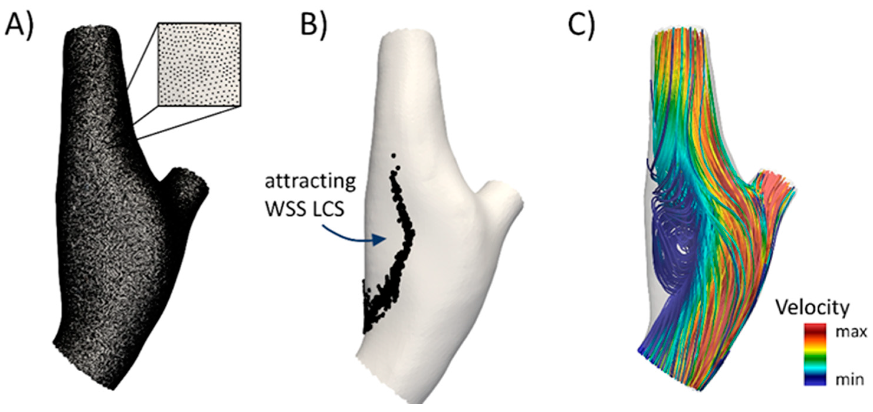
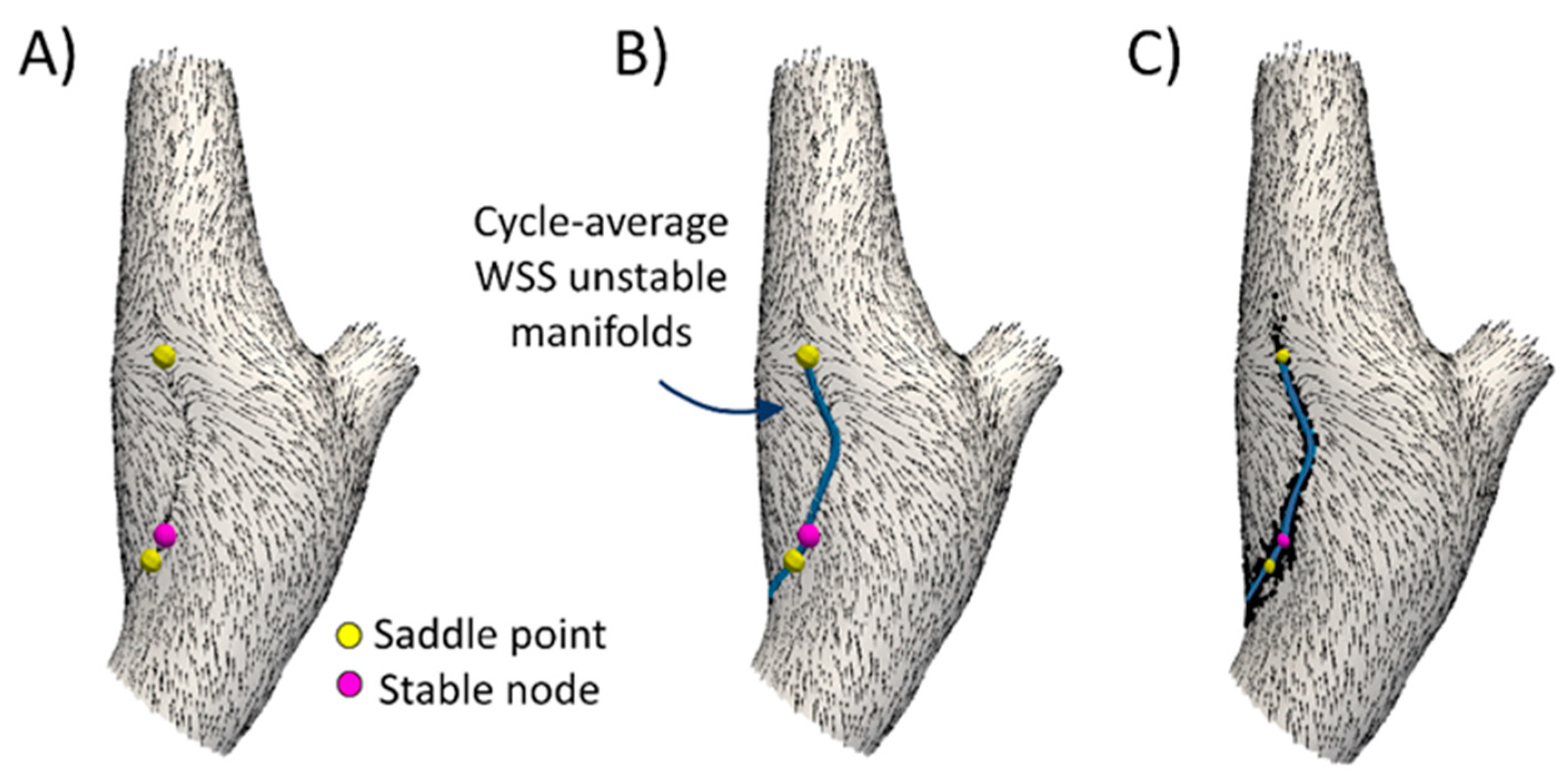
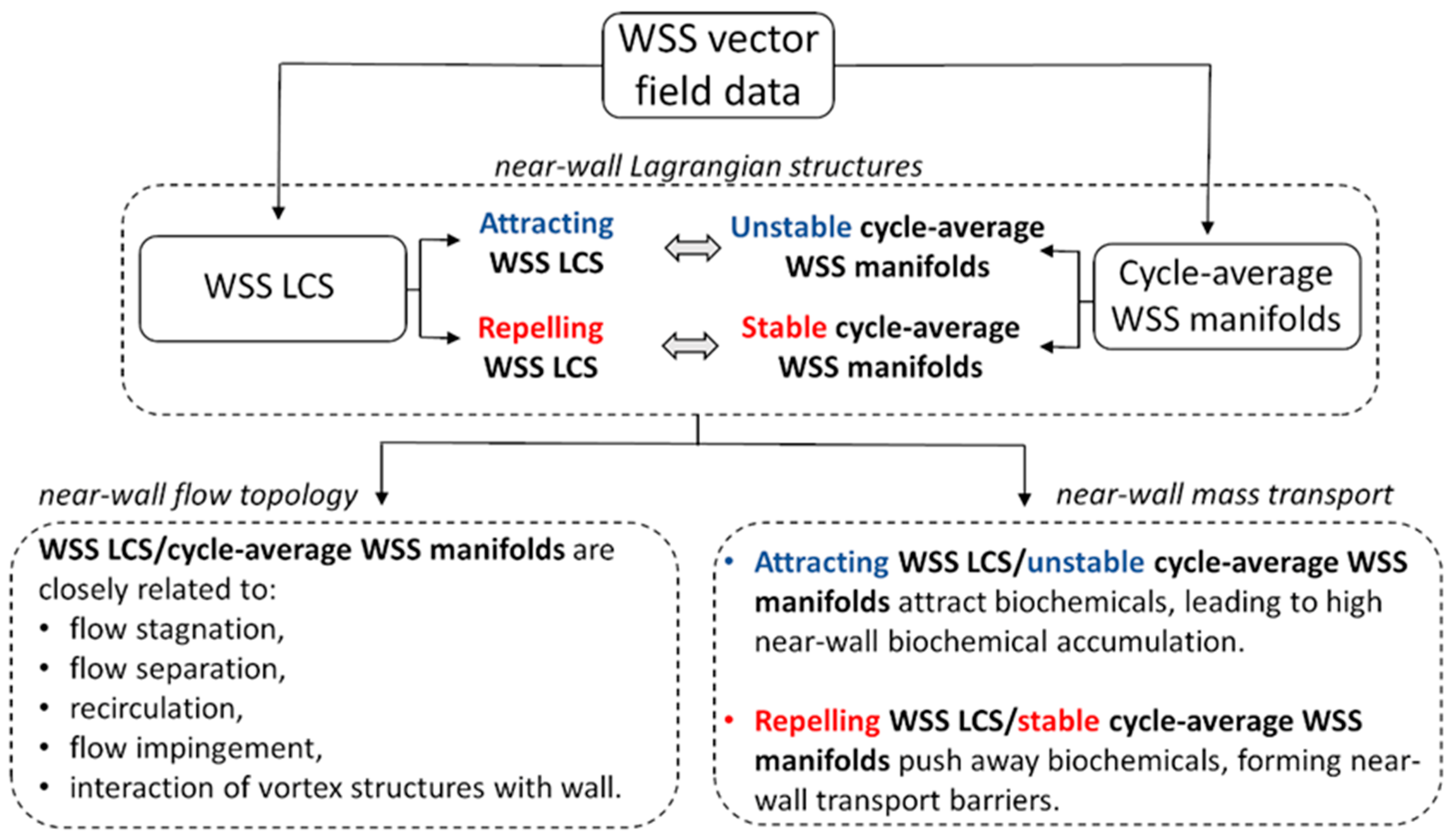
3.3. LCS Application to Near-Wall Flow Features

Recently, in the study of cardiovascular flows, the concept of LCS has been extended to analyze the near-wall flow topology, i.e., the topology of the flow field close to the luminal surface of arteries. The rationale is in the well-established involvement of near-wall mass transport in most of the processes concurring to determine vascular pathophysiology [5]: in the near-wall region, blood flow regulates the local biotransport processes and imparts mechanical shear stress on the endothelium (i.e., the WSS), which in turn regulates important developmental, homeostatic, and adaptive mechanisms in arteries, as well as susceptibility to and progression of atherosclerosis [1].

Based on theory, it has been demonstrated [60] that the WSS vector field can be scaled to provide a first-order approximation for the near-wall blood flow velocity vector field as follows:

$${\mathit{u}}_{\pi }=\frac{\mathit{\tau }\delta n}{\mu }+\mathrm{O}\left(\delta n^2\right),$$

(12)

where ${\mathit{u}}_{\pi }\in {ℝ}^3$ is the near-wall velocity, $\mathit{\tau }\in {ℝ}^3$ represents the WSS vector field, $\mu$ is the dynamic viscosity, and $\delta n$ is the distance from the wall where the velocity is evaluated. By construction, the vector field in Equation (12) is defined on the luminal surface of the vessel, and it represents the near-wall velocity, as the velocity is zero on the surface itself due to the no-slip condition. The LCS underlying theory described in Section 3.1 can be extended to analyze the near-wall flow topology by using the expression of near-wall velocity ${\mathit{u}}_{\pi }$ (given by Equation (12)) in Equation (1). Such near-wall Lagrangian structures, computed from the WSS vector field, are referred to as WSS LCS [15].

Computationally, WSS LCS can be identified on the luminal surface of the vessel by numerically integrating a high number of luminal surface tracer particles, applying the procedure described in the first part of Section 3.1. In detail, attracting and repelling WSS LCS can be traced out with forward and backward time integration of surface tracer particles based on the near-wall blood flow velocity (Equation (12)), respectively.

The recent interest in WSS LCS from the cardiovascular fluid mechanics research community was driven by WSS LCS ability to highlight blood flow features associated with vascular disease initiation and progression, like flow stagnation, separation, recirculation, flow impingement, and the interaction of vortex structures with the vascular wall [19,61,62] These blood flow features have been classified as “aggravating flow events”, as they trigger biological processes leading to the development or progression of vascular disease [2,17]. An example of attracting WSS LCS on the luminal surface of a patient-specific computational hemodynamic model of carotid bifurcation is presented in Figure 5. Details on the carotid bifurcation hemodynamic modeling are reported elsewhere [9,14,20,63]. In this specific case, luminal surface tracer particles (Figure 5A) are numerically integrated in forward time. The resulting LCS is located at the carotid bulb, a region characterized by flow disturbances (slow, recirculating blood flow) promoting atherosclerosis [2,4]. In detail, the attracting WSS LCS provides the boundary at the luminal surface of the slow vortex structure formed inside the carotid bulb (Figure 5C, where the recirculation region is highlighted visualizing the streamlines of the cycle-average velocity vector field).

In addition, the shear forces exerted by the streaming blood flow in the near-wall region on the endothelium affect biotransport processes, i.e., the transport of biochemicals through the subendothelial layer [22]. Biotransport is of paramount importance in many cardiovascular processes, including the initiation of atherosclerosis and thrombogenesis [23]. In general, cardiovascular mass transport is investigated in silico by coupling the governing equations of motion, the Navier–Stokes equations, with the advection–diffusion equation, given by:

$$\frac{dC}{d\mathrm{t}}+\mathit{u}· \nabla C-D{\nabla }^{2}C=0,$$

(13)

where $C$ is a non-dimensional concentration of the species transported in the domain, $\mathit{u}$ is the fluid velocity vector, and $D$ is the mass diffusion coefficient. However, high computational costs are associated with the class of numerical simulations used to accurately solve the near-wall transport and blood-wall transfer [64,65], making this approach expensive in hemodynamics applications. To overcome this limitation, and based on the well-established role that WSS plays in conditioning the permeability of the endothelium and the near-wall mass transport process, recent studies [15,18] have brilliantly demonstrated that WSS LCS can be used as a template for near-wall mass transport. This allows reduction of the computational effort needed to solve the full transport problem, represented by Equation (13) [15]. In particular, it has been demonstrated that attracting WSS LCS attract biochemicals, leading to high near-wall concentration in their neighborhood, whereas repelling WSS LCS have been shown to act as near-wall transport barriers [15,17].

In the context of cardiovascular flows, it has been recently demonstrated that attracting/repelling WSS LCS on the luminal surface of an artery match the unstable/stable manifolds of the cycle-average WSS vector field [15,18], defined as:

$$\overline{\mathit{\tau }}=\frac{1}{T}{{\displaystyle \int }}_0^T\mathit{\tau }\left(\mathit{x},t\right)dt,$$

(14)

where $\mathit{\tau }$ is the instantaneous local WSS value and T is the time duration of the cardiac cycle. Technically, the first step in the topological analysis of cycle-average WSS at the luminal surface of a vessel is the identification of WSS fixed points. The exact position of WSS fixed points can be identified by computing, e.g., the Poincaré index, as explained in Section 2. Then, the cycle-average WSS field around a fixed point ${\mathit{x}}_{fp}$, according to Equation (5), by linearization can be expressed as:

$$\overline{\mathit{\tau }}\left(\mathit{x}\right)=\overline{\mathit{\tau }}\left({\mathit{x}}_{fp}\right)+J\left({\mathit{x}}_{fp}\right)\left(\mathit{x}-{\mathit{x}}_{fp}\right),$$

(15)

where $J$ is the Jacobian matrix of $\overline{\mathit{\tau }}$ (see Equation (14)). The identified WSS fixed points can be classified according to their nature (i.e., saddle, node, or focus, Figure 1A) by analyzing the eigenvalues of the Jacobian matrix $J$ of $\overline{\mathit{\tau }}$ (Table 1), as described in Section 2. Note that the WSS vector field is embedded in a three-dimensional space even if it lies in a two-dimensional space (the luminal surface of a vessel). To perform a two-dimensional analysis, two strategies are possible. In the first strategy, a projection of the vector field into two orthogonal directions (hence, in a two-dimensional space) is needed. In the second one, avoiding the projection of the vector field (and thus reducing the computational steps), a three-dimensional analysis is performed, thus obtaining three eigenvalues of the Jacobian matrix, with one of them having a value close to zero. Then, the eigenvalue-based analysis for the WSS fixed points classification considers only the two eigenvalues different from zero.

Saddle-type fixed points are of particular interest, since typically a stable or unstable manifold starts from a saddle point and vanishes into a source or sink, respectively, as depicted in Figure 1B. Saddle point locations (where the Poincaré index is −1 and the eigenvalues are real with different signs) are perturbed along the positive eigenvector of $J$ in two opposite directions, obtaining two initial conditions [18,61]. Unstable manifolds can be traced out by numerically integrating $\overline{\mathit{\tau }}$ from these initial conditions in forward time until trajectories reach a stable fixed point (sink configuration) or leave the domain. Similarly, stable manifolds are delineated by integrating $\overline{\mathit{\tau }}$ in backward time starting from the perturbation of saddle point locations along the negative eigenvector of $J$ until trajectories reach an unstable fixed point (source configuration) or leave the domain.

An example of unstable manifolds of cycle-average WSS on the luminal surface of a patient-specific computational hemodynamic model of carotid bifurcation is presented in Figure 6. Details on carotid bifurcation hemodynamic modeling are reported elsewhere [9,14,20,63]. WSS fixed points were identified by computing the Poincaré index (Figure 6A), and subsequently, unstable manifolds were traced out by applying Runge-Kutta 4-5 numerical integration schemes (Figure 6B). By visual inspection of Figure 6C, it can be appreciated that cycle-average WSS unstable manifolds co-localize with attracting WSS LCS, confirming the capability of the latter to identify critical lines of the WSS field.

The analysis of cycle-average WSS fixed points and manifolds has been applied to analyze cardiovascular flows. Arzani et al. [18] used WSS LCS from stable and unstable manifolds of cycle-average WSS on patient-specific computational hemodynamics models of AAAs, carotid arteries, cerebral aneurysms, and coronary aneurysms to characterize near-wall flow topology and biochemical transport. Farghadan et al. [16] used WSS topology and magnitude analysis to predict surface concentration patterns in cardiovascular transport problems by computing WSS LCS from manifolds of cycle-average WSS in image-based coronary and carotid artery models. Mahmoudi et al. [21] studied the near-wall transport of some of the prominent biochemicals contributing to the initiation and progression of atherosclerosis in computational hemodynamic models of the coronary artery, highlighting the strength of cycle-average WSS LCS as a template for luminal surface concentration and flux patterns of biochemicals transported with blood.

Summarizing, the Lagrangian approach for identifying near-wall topological features is schematized in Figure 7, where the link between attracting/repelling WSS LCS with unstable/stable cycle-average WSS manifolds, respectively, is highlighted. In addition, Figure 7 presents a brief summary of the link between Lagrangian-based near-wall flow topology and mass transport. For a more in-depth analysis, the interested reader can refer to recent literature [15,17,18,21] where the link between WSS LCS, cycle-average WSS manifolds, and biochemical transport in cardiovascular flows is unambiguously documented.

4. Eulerian Approach

4.1. Volume Contraction Theory

From a Eulerian perspective, the volume contraction theory provides a simple alternative way to analyze the behavior of a dynamical system. Contrarily to Lagrangian-based approaches, the Eulerian perspective considers vector field properties at each point in space and time. The here-presented volume contraction theory, based on fluid mechanics and differential geometry, is focused on the temporal change of an elemental volume (of fluid, for the case of interest) in the phase space of a dynamical system (fluid flow, for the case of interest). Let $V\left(t\right)$ be an arbitrary volume in the phase space of the dynamical system defined in Equation (1). Let $S\left(t\right)$ be a closed surface enclosing the volume $V\left(t\right)$, i.e., such that $S\left(t\right)=\delta V\left(t\right)$. $S\left(t\right)$ evolves during the time interval $dt$ resulting in a contraction or expansion of the volume, as depicted in Figure 8. The rate of volume variation, which we will call volume contraction rate in the following, can be expressed as follows as a consequence of the application of the Gauss theorem:

$$\frac{dV\left(t\right)}{dt}={\displaystyle \int }{{\displaystyle \int }}_S^{}\mathit{u}·\mathit{n} dS={\displaystyle \int }{\displaystyle \int }{{\displaystyle \int }}_V^{}\nabla ·\mathit{u} dV,$$

(16)

where $\mathit{u}$ is the vector field defined in Equation (1) and $\mathit{n}$ is the unit normal to the surface S (Figure 8). Shrinking the near-wall volume $V$ to a point, it can be written:

$$\underset{V\to 0}{\lim }\frac{1}{V}\frac{dV\left(t\right)}{dt}=\underset{V\to 0}{\lim }\frac{1}{V}{\displaystyle \int }{\displaystyle \int }{{\displaystyle \int }}_V^{}\nabla ·\mathit{u} dV=\left(\nabla ·\mathit{u}\right).$$

(17)

Equation (17) clearly shows that in the limit as $V$ approaches zero, the local value of vector $\mathit{u}$ divergence is equal to its total flux per unit volume.

In general, in non-conservative dynamical systems, the volume of phase space is not preserved, as it can contract or expand. Thus, trajectories tend toward a lower-dimensional subset of phase space. From Equation (17), the volume contraction rate Λ(x,t) of a n-dimensional system, representing the rate of separation of infinitesimal close trajectories, can be obtained as:

$$\mathsf{\Lambda }\left(\mathit{x},t\right)=\nabla ·\mathit{u}\left(\mathit{x},t\right)=tr J\left(\mathit{u}\right)={\displaystyle \sum }_{\mathit{i}=\mathbf{1}}^{\mathit{n}}{\lambda }_{\mathit{i},}$$

(18)

where $tr J\left(\mathit{u}\right)$ is the trace of the Jacobian matrix of vector field $\mathit{u}$ and ${\lambda }_{\mathit{i}}$ are its eigenvalues. Physically, the Jacobian matrix describes how a small change at a starting point ${\mathit{x}}_{\mathbf{0}}$propagates to the final point of the flow map ${\mathsf{\Phi }}_{t_0}^t\left({\mathit{x}}_{\mathbf{0}}\right)$ of Equation (3). In this sense, Equation (18) represents the sum of the Lyapunov exponents of Equation (8).

4.2. Eulerian-Based Approach for WSS Topological Skeleton Identification

It has been recently demonstrated [19] that the application of the volume contraction theory to cardiovascular flows allows the analysis of the WSS topological skeleton on the luminal surface of a vessel through the direct calculation of the WSS divergence. Briefly, considering the expression of the near-wall blood flow velocity vector ${\mathit{u}}_{\pi }$ given in Equation (12) and substituting it in Equation (17), it follows that:

$$\underset{V\to 0}{\lim }\frac{1}{V}\frac{dV\left(t\right)}{dt}=\underset{V\to 0}{\lim }\frac{\delta n}{V\mu }{\displaystyle \int }{\displaystyle \int }{{\displaystyle \int }}_V^{}\nabla ·\mathit{\tau } dV=\left(\nabla ·\mathit{\tau }\right).$$

(19)

Based on Equation (19), the WSS divergence gives practical information about the WSS topological skeleton. Note that in general, the WSS vector field defined at the luminal surface of a vessel is not conservative, even in the case of incompressible flows.

Contextualizing the physical meaning of Equation (19) to the study of the phenomena at the interface between blood flow and vessel wall, it can be observed that as the divergence represents the volume density of the outward flux of a vector field from an infinitesimal volume around a given point:

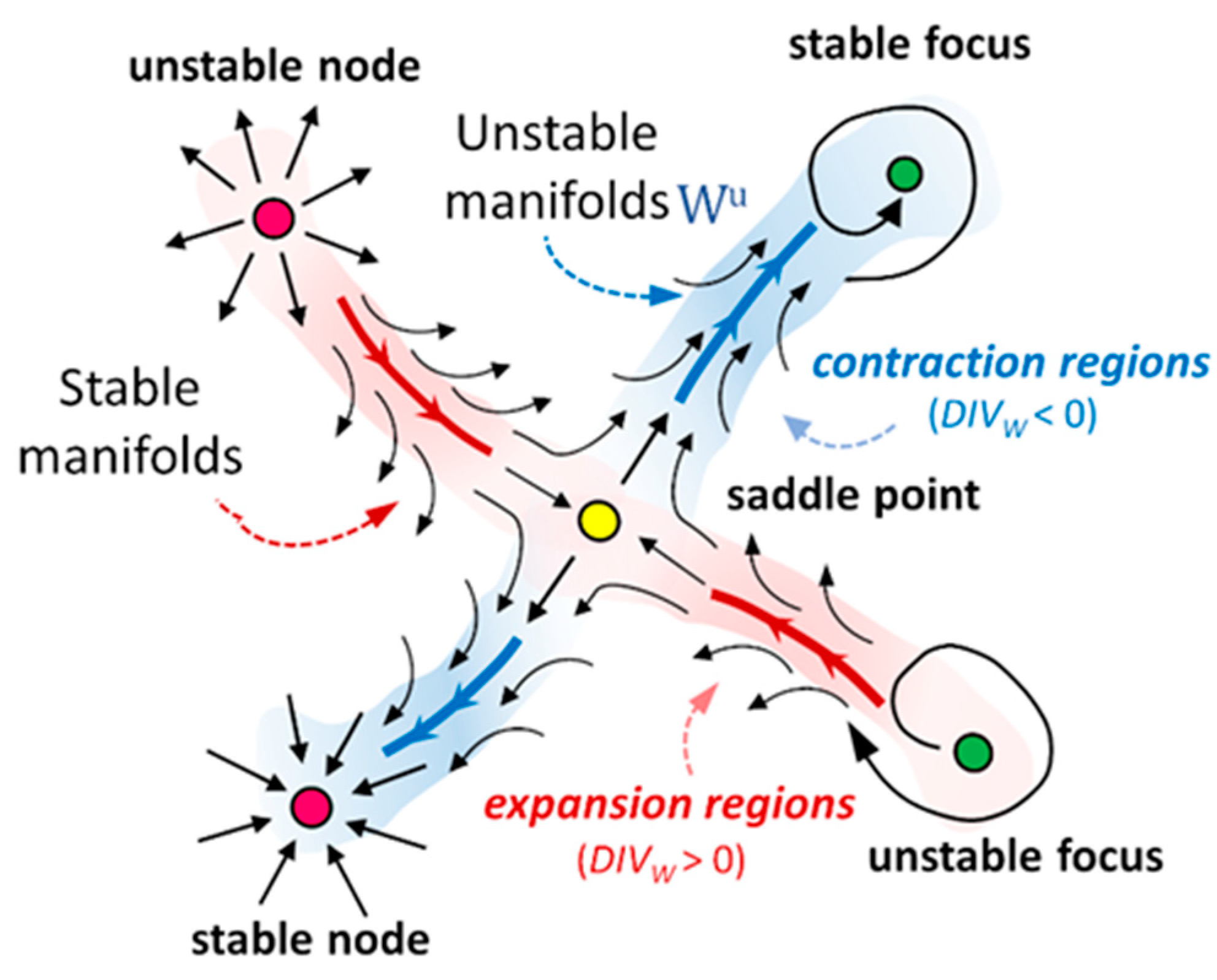
• a local positive value of the divergence of the WSS field at the luminal surface means that locally shear forces exert an expansion action on the endothelium;
• a local negative value of the divergence of the WSS field at the luminal surface means that locally shear forces exert a contraction action on the endothelium.

In general, the application of the volume contraction theory to the analysis of a dynamical system faces one limitation in cases where the distance between two neighboring trajectories increases/decreases in spite of a negative/positive value of divergence, respectively. As WSS divergence depends by construction upon the algebraic summation of the magnitude of the single gradients of WSS vector components, in some cases, it might fail to properly identify WSS expansion/contraction configuration patterns. In fact, these regions describe specific directional arrangements of the vectors, but both variations in magnitude and in direction are accounted for in the divergence. To overcome this limitation, which could markedly affect the application of the Eulerian-based approach to study WSS manifolds in cardiovascular flows, the use of the divergence of the normalized WSS vector field has been recently proposed [19]:

$$DI{V}_W=\nabla ·{\mathit{\tau }}_u=\nabla ·\left(\frac{\mathit{\tau }}{\left|\mathit{\tau }\right|}\right),$$

(20)

where ${\mathit{\tau }}_u$ is the WSS unit vector. Equation (20) can be used to encase the connections between fixed points, i.e., manifolds, identify basins of attraction, and subdivide the domain into different vector field behaviors. Then, in the light of the above and as depicted in Figure 9, luminal surface regions characterized by negative values of $DI{V}_W$ are referred to as contraction regions and approximate unstable manifolds. Similarly, regions at the luminal surface characterized by positive values of $DI{V}_W$ are referred to as expansion regions and approximate stable manifolds (Figure 9).

To complete the Eulerian-based WSS topological skeleton analysis, once WSS manifolds have been identified using $DI{V}_W$, the WSS fixed point location can be carried out using the Poincaré index, as in the Lagrangian-based analysis (as described in Section 2). Then, the eigenvalues of the Jacobian matrix of the WSS vector field can be used to distinguish between a node or a focus and between the attractive or repelling nature of a fixed point, as described in Section 2 in general terms (Table 1) and in Section 3.3 for the specific case of a WSS vector field defined on the luminal surface of a vessel.

An example of Eulerian-based topological skeleton analysis of the cycle-average WSS field on the luminal surface of a patient-specific computational hemodynamic model of carotid bifurcation is presented in Figure 10A. Details on carotid bifurcation hemodynamic modeling are reported elsewhere [9,14,20,63]. WSS fixed points were identified and classified by computing the Poincaré index and eigenvalues of the Jacobian matrix, respectively, whereas contraction/expansion regions were identified by computing the divergence of the normalized cycle-average WSS vector field. By visual inspection of Figure 10B, it can be noted that cycle-average WSS contraction regions co-localize with cycle-average WSS unstable manifolds, traced out by integrating cycle-average WSS starting from saddle point positions, thus confirming the capability of the contraction regions to encase WSS manifolds.

The Eulerian-based approach to analyze the WSS topological skeleton can be easily implemented. It requires only single snapshots of the WSS vector field, and the post-processing algorithms, based on a robust theory, are easily reproduced. This approach does not need the Lagrangian surface transport computation, as required for Lagrangian-based and integrated trajectory-based methods, thus reducing computational effort. Furthermore, it is characterized by modularity in the sense that the method can be applied only for the purpose of fixed point identification and/or classification or only for contraction/expansion region identification.

4.3. Application of the Eulerian-Based Method for WSS Topological Skeleton Analysis to Cardiovascular Flows

The described Eulerian-based method to identify the WSS topological skeleton on the luminal surface of an artery can be easily applied (1) to cycle average WSS vectors (defined in Equation (14) in Section 3.3) and (2) to instantaneous WSS vectors along the cardiac cycle.

The cycle-average WSS topological skeleton highlights blood flow features associated with vascular disease development, and it is strongly related to arterial near-wall mass transport. In detail, on the one hand, contraction/expansion regions of cycle-average WSS vectors, because of their capability to encase unstable/stable cycle-average WSS manifolds, can be used to identify biochemical concentration patterns at the arterial luminal surface. On the other hand, the instantaneous WSS topological skeleton allows analyzing the unsteady nature of WSS fixed points and contraction/expansion regions. In detail, instantaneous WSS fixed points may have a potential impact on the endothelial cells (ECs) function. By definition, a WSS fixed point represents a focal point on the luminal surface of a vessel where WSS vanishes, and low WSS is a biomechanical factor involved in vascular dysfunction. In light of this, quantitative descriptors of WSS fixed points residence times along the cardiac cycle were proposed [17,19], aiming at characterizing their unsteady nature. In detail, a WSS fixed point residence time, that for each surface element measures the accumulated amount of time that WSS fixed points spend inside that element, weighted by the sum of the absolute values of the eigenvalues of the instantaneous WSS Jacobian matrix, was proposed elsewhere [17]. More recently, a different formulation for quantifying WSS fixed points was proposed [19] where the local residence time of WSS fixed points were weighted by the absolute value of the sum of the eigenvalues of the WSS Jacobian matrix (i.e., according to Equation (18), the absolute value of the WSS divergence, representing the strength of the contraction/expansion of the WSS around the fixed point). In mathematical terms:

$$RT{\nabla }_{{\mathit{x}}_{fp}}\left(e\right)=\frac{\overline{A}}{A_e}\frac{1}{T}\underset{0}{\overset{T}{{\displaystyle \int }}}{\mathbb{I}}_e\left({\mathit{x}}_{fp},t\right)|{(\nabla ·\mathit{\tau })}_e|dt,$$

(21)

where ${\mathit{x}}_{fp}$ is the location of a WSS fixed point at time$t \in \left[0,T\right]$, $T$ is the cardiac cycle duration, e is the generic triangular element of the superficial mesh of area $A_e$, $\overline{A}$ is the average surface area of all triangular elements of the superficial mesh, ${\mathbb{I}}_e$is the indicator function (equal to 1 if ${\mathit{x}}_{fp}\in e$, 0 otherwise) and ${(\nabla ·\mathit{\tau })}_e$ is the instantaneous WSS divergence value, representing the local strength of the contraction/expansion of the WSS around the considered fixed point. Roughly speaking, Equation (21) allows quantifying the fraction of the cardiac cycle for which a generic triangle mesh surface element e on the vessel luminal surface hosted as a fixed point, weighting the residence time by the strength of the local contraction/expansion action.

Furthermore, the strength and the nature of WSS contraction and expansion action on the ECs lining the luminal surface, as identified by WSS contraction/expansion regions, is expected to have biological consequences linked to vascular pathophysiology. In particular, the exposure to high variability of WSS contraction and expansion action may mechanically induce a recurring variation in EC stimulation along the cardiac cycle, with consequent widening cell–cell junctions and associated increased endothelium permeability and EC dysfunction and apoptosis [7,66]. The amount of variation in the WSS contraction/expansion action exerted at the luminal surface of a vessel along the cardiac cycle can be quantified using the quantity topological shear variation index ($TSVI$) [24]:

$$TSVI={\left\{\frac{1}{T}{{\displaystyle \int }}_0^T{\left[DI{V}_W-\overline{DI{V}_W} \right]}^2 dt\right\}}^{1/2}.$$

(22)

Equation (22) allows localizing regions on the vessel luminal surface exposed to large variations in WSS contraction/expansion action exerted by the flowing blood along the cardiac cycle.

An example of the distribution of WSS fixed point weighted residence time (Equation (21)) and the topological shear variation index (Equation (22)) on the luminal surface of a patient-specific computational hemodynamic model of carotid bifurcation is presented in Figure 11. Details on the carotid bifurcation hemodynamic modeling are reported elsewhere [9,14,20,63]. From Figure 11, it emerged that the highest $RT{\nabla }_{{\mathit{x}}_{fp}}\left(e\right)$ values and highest variation in the contraction/expansion action exerted by the WSS along the cardiac cycle were mainly located at the carotid bulb and around the bifurcation apex.

Interestingly, very recent studies highlighted a link between WSS contraction/expansion variability along the cardiac cycle and aggravating biological events at the arterial wall. In particular, De Nisco et al. [24] applied the Eulerian-based approach for the analysis of the WSS topological skeleton for personalized computational hemodynamic models of ascending thoracic aorta aneurysm (ATAA) and healthy aorta, reporting that: (1) the different spatiotemporal heterogeneity characterizing the ATAA and healthy hemodynamics markedly reflect on their WSS topological skeleton features; (2) a link emerged between the variability of the contraction/expansion action exerted by WSS on the endothelium (as quantified by the $TSVI$) along the cardiac cycle and ATAA wall stiffness. Morbiducci et al. [20] demonstrated in a longitudinal study integrating clinical data with computational hemodynamics that WSS topological skeleton features quantified by the TSVI independently predicted long-term restenosis after carotid bifurcation endarterectomy.

5. Future Directions

The translation into clinical settings of the WSS topological skeleton is hampered by several barriers that add up to those affecting in general the translation of computational hemodynamics and the derived knowledge, as discussed elsewhere [67]. Specifically, as a first step, the analysis of the topological skeleton needs to be distilled into intuitive, clinically relevant criteria. To this aim, only semi-quantitative results are obtained from the definition of fixed points and stable/unstable manifolds, consisting of contraction/expansion regions. However, quantitative results can be obtained by focusing on specific features by using ad-hoc topological skeleton descriptors, such as the fixed point weighted residence time $RT{\nabla }_{x_{fp}}\left(e\right)$ (Equation (21)) or the topological shear variation index, TSVI (Equation (22)). Then, the definition of clinically relevant criteria based on the WSS topological descriptors require cut-off values for an effective translation into the clinic. These cut-off values need to be accurately defined and tested in terms of performance including accuracy, sensitivity, specificity, and positive predictive value, among others. Therefore, the determination of cut-off values requires adequate statistical power, obtained usually through multiple prospective, randomized trials. Moreover, the endpoint to be predicted should be clearly defined, as different endpoints correspond to different cut-off values.

In the perspective of an effective translation into the clinic of quantitative topological skeleton features, in a previous study [20], we proved that exposure to high values of both descriptors $RT{\nabla }_{x_{fp}}\left(e\right)$ and TSVI was correlated with intima-media thickness (a marker of vascular disease) at 60 month follow-ups in carotid bifurcations after carotid endarterectomy. To determine the cut-off values of the descriptors, a pooled distribution for each descriptor was calculated from 46 models of healthy carotid bifurcation. The 80th percentile of those distributions was then used. This approach allowed definition of the cut-off values for abnormally high values of $RT{\nabla }_{x_{fp}}\left(e\right)$ or the TSVI.

It is evident that cut-off values are specific to the vascular region and to the predicted endpoint and therefore cannot be extrapolated to other conditions. In the future, the continuous improvements in imaging and data acquisition, the increasing availability of computational power, and the development of more and more efficient and robust methodologies for blood flow modeling are expected to accelerate the translation into the clinic of the analysis of the WSS topological skeleton. Our paper aims to give the methodological basis to tackle these future efforts.

6. Conclusions

The need for the identification of hemodynamic coherent structures in blood vessels is dictated by the so-called hemodynamic risk hypothesis, suggesting a major role of flow disturbances in vascular pathophysiology [2]. The action of fluid forces on the endothelial mechanosensors and biochemical machinery has been historically explained in terms of WSS [3,4]. However, only moderate (and sometimes contradictory) associations between vascular disease and WSS-based descriptors have emerged to date, motivating a more in-depth analysis of the fluid near-wall transport phenomena. In this sense, the capability of the WSS topological skeleton to capture features reflecting cardiovascular flow complexity [17,18,19,20] and having a direct link to adverse vascular biological events has recently attracted a strong research interest. In this regard, recent studies have demonstrated that the cycle-average WSS topological skeleton governs the near-wall biochemical transport in arteries [15,16,18], a process linked to, e.g., endothelium-mediated vasoregulation, thrombosis, and atherosclerosis [23]. Furthermore, evidence about the role of WSS topological skeleton features in vascular pathophysiology emerged from very recent studies suggesting a direct link between WSS topological skeleton features and, e.g., aortic wall stiffness [24] and late restenosis in endarterectomized carotid arteries [20].

Motivated by the need to characterize more precisely the WSS phenotype(s) linked to aggravating biological events, here we provided an overview of the theoretical and methodological basis for analyzing the WSS topological skeleton in cardiovascular flows. In detail, the present study is intended to: (1) promote the application of WSS topological skeleton analysis to cardiovascular flows, aiming at elucidating the role that peculiar WSS features play in vascular pathophysiology; (2) facilitate the reproducibility and comparability of results from WSS topological skeleton analyses among different studies; (3) confirm its potential as a tool for increasing the chance of elucidating the mechanistic link between flow disturbance and clinical outcomes when applied to real-world clinical data.

Here, both WSS topological skeleton Lagrangian- and Eulerian-based methods currently adopted in the literature are presented. Lagrangian-based approaches start from the processing of Eulerian data, which represent the typical outputs of current in vivo (e.g., phase contrast MRI), in vitro (e.g., particle image velocimetry), and computational methods used for the investigation of cardiovascular flows. On the one hand, Lagrangian approaches are particularly useful for revealing the global organization of the vector field and characterizing its evolution over time, making the relevant features easy to detect by visual inspection, as they offer effective three-dimensional (or even four-dimensional, i.e., including time) visualizations. On the other hand, Lagrangian techniques rely on the numerical integration of particle trajectories, requiring sufficiently resolved data in both time and space, thus, in principle, making such methods computationally expensive and time consuming [29]. Moreover, adopting a Lagrangian approach may result in a poor control over the zone of investigation, which is determined by particle motion and accumulation. For this reason, it can also be difficult to get a complete picture of the flow at specific time instants. Furthermore, the influence of particle distribution and of particle seeding schemes on quantities of interest is poorly investigated.

In contrast, Eulerian-based approaches usually simplify the data analysis workflow, as they can be directly applied to the output given by the main current techniques used for the investigation of cardiovascular flows (e.g., phase contrast MRI, CFD data). Moreover, they usually have a simpler definition, making their implementation easy and characterized by a reduced computational cost. More importantly, they can give a picture of the entire vector field. However, the inherent unsteady nature of the hemodynamic vector fields (e.g., velocity, WSS) can make the characterization of the dynamic evolution of the vector field features difficult with Eulerian-based approaches.

In conclusion, the theoretical background of the advanced methods of analysis of the WSS presented here and the recent findings related to their application to cardiovascular flows support their use to further elucidate the cause–effect relationships at the basis of the links between local hemodynamics and vascular disease. Based on the reported evidence about the physiological significance of the WSS topological skeleton in cardiovascular flows, its application in future studies, including longitudinal data, biological mechanism, and mechanobiology studies, is strongly encouraged and warranted.

References

1. Kwak, B.R.; Bäck, M.; Bochaton-Piallat, M.-L.; Caligiuri, G.; Daemen, M.J.A.P.; Davies, P.F.; Hoefer, I.E.; Holvoet, P.; Jo, H.; Krams, R.; et al. Biomechanical factors in atherosclerosis: Mechanisms and clinical implications. Eur. Heart J. 2014, 35, 3013–3020. [Google Scholar] [CrossRef] [PubMed]
2. Morbiducci, U.; Kok, A.M.; Kwak, B.R.; Stone, P.H.; Steinman, D.A.; Wentzel, J.J. Atherosclerosis at arterial bifurcations: Evidence for the role of haemodynamics and geometry. Thromb. Haemost. 2016, 115, 484–492. [Google Scholar] [CrossRef]
3. Malek, A.M.; Alper, S.L.; Izumo, S. Hemodynamic shear stress and its role in atherosclerosis. J. Am. Med. Assoc. 1999, 282, 2035–2042. [Google Scholar] [CrossRef]
4. Zarins, C.K.; Giddens, D.P.; Bharadvaj, B.K.; Sottiurai, V.S.; Mabon, R.F.; Glagov, S. Carotid bifurcation atherosclerosis. Quantitative correlation of plaque localization with flow velocity profiles and wall shear stress. Circ. Res. 1983, 53, 502–514. [Google Scholar] [CrossRef] [Green Version]
5. Caro, C.G.; Fitz-Gerald, J.M.; Schroter, R.C. Atheroma and arterial wall shear. Observation, correlation and proposal of a shear dependent mass transfer mechanism for atherogenesis. Proc. R. Soc. Lond. Ser. B Biol. Sci. 1971, 177, 109–159. [Google Scholar] [CrossRef]
6. Ku, D.N.; Giddens, D.P.; Zarins, C.K.; Glagov, S. Pulsatile flow and atherosclerosis in the human carotid bifurcation. Positive correlation between plaque location and low oscillating shear stress. Arteriosclerosis 1985, 5, 293–302. [Google Scholar] [CrossRef] [Green Version]
7. Wang, C.; Baker, B.M.; Chen, C.S.; Schwartz, M.A. Endothelial cell sensing of flow direction. Arterioscler. Thromb. Vasc. Biol. 2013, 33, 2130–2136. [Google Scholar] [CrossRef] [Green Version]
8. Peiffer, V.; Sherwin, S.J.; Weinberg, P.D. Does low and oscillatory wall shear stress correlate spatially with early atherosclerosis? A systematic review. Cardiovasc. Res. 2013, 99, 242–250. [Google Scholar] [CrossRef]
9. Gallo, D.; Bijari, P.B.; Morbiducci, U.; Qiao, Y.; Xie, Y.J.; Etesami, M.; Habets, D.; Lakatta, E.G.; Wasserman, B.A.; Steinman, D.A. Segment-specific associations between local haemodynamic and imaging markers of early atherosclerosis at the carotid artery: An in vivo human study. J. R. Soc. Interface 2018, 15. [Google Scholar] [CrossRef] [Green Version]
10. Hoogendoorn, A.; Kok, A.M.; Hartman, E.M.J.; de Nisco, G.; Casadonte, L.; Chiastra, C.; Coenen, A.; Korteland, S.A.; Van der Heiden, K.; Gijsen, F.J.H.; et al. Multidirectional wall shear stress promotes advanced coronary plaque development: Comparing five shear stress metrics. Cardiovasc. Res. 2020, 116, 1136–1146. [Google Scholar] [CrossRef]
11. Kok, A.M.; Molony, D.S.; Timmins, L.H.; Ko, Y.-A.; Boersma, E.; Eshtehardi, P.; Wentzel, J.J.; Samady, H. The influence of multidirectional shear stress on plaque progression and composition changes in human coronary arteries. EuroIntervention 2019, 15, 692–699. [Google Scholar] [CrossRef] [Green Version]
12. Timmins, L.H.; Molony, D.S.; Eshtehardi, P.; McDaniel, M.C.; Oshinski, J.N.; Giddens, D.P.; Samady, H. Oscillatory wall shear stress is a dominant flow characteristic affecting lesion progression patterns and plaque vulnerability in patients with coronary artery disease. J. R. Soc. Interface 2017, 14. [Google Scholar] [CrossRef] [PubMed]
13. Colombo, M.; He, Y.; Corti, A.; Gallo, D.; Casarin, S.; Rozowsky, J.M.; Migliavacca, F.; Berceli, S.; Chiastra, C. Baseline local hemodynamics as predictor of lumen remodeling at 1-year follow-up in stented superficial femoral arteries. Sci. Rep. 2021, 11, 1613. [Google Scholar] [CrossRef]
14. Gallo, D.; Steinman, D.A.; Morbiducci, U. Insights into the co-localization of magnitude-based versus direction-based indicators of disturbed shear at the carotid bifurcation. J. Biomech. 2016, 49, 2413–2419. [Google Scholar] [CrossRef]
15. Arzani, A.; Gambaruto, A.M.; Chen, G.; Shadden, S.C. Lagrangian wall shear stress structures and near-wall transport in high-Schmidt-number aneurysmal flows. J. Fluid Mech. 2016, 790, 158–172. [Google Scholar] [CrossRef] [Green Version]
16. Farghadan, A.; Arzani, A. The combined effect of wall shear stress topology and magnitude on cardiovascular mass transport. Int. J. Heat Mass Transf. 2019, 131, 252–260. [Google Scholar] [CrossRef]
17. Arzani, A.; Shadden, S.C. Wall shear stress fixed points in cardiovascular fluid mechanics. J. Biomech. 2018, 73, 145–152. [Google Scholar] [CrossRef]
18. Arzani, A.; Gambaruto, A.M.; Chen, G.; Shadden, S.C. Wall shear stress exposure time: A Lagrangian measure of near-wall stagnation and concentration in cardiovascular flows. Biomech. Model. Mechanobiol. 2017, 16, 787–803. [Google Scholar] [CrossRef]
19. Mazzi, V.; Gallo, D.; Calò, K.; Najafi, M.; Khan, M.O.; De Nisco, G.; Steinman, D.A.; Morbiducci, U. A Eulerian method to analyze wall shear stress fixed points and manifolds in cardiovascular flows. Biomech. Model. Mechanobiol. 2020, 19, 1403–1423. [Google Scholar] [CrossRef]
20. Morbiducci, U.; Mazzi, V.; Domanin, M.; De Nisco, G.; Vergara, C.; Steinman, D.A.; Gallo, D. Wall Shear Stress Topological Skeleton Independently Predicts Long-Term Restenosis After Carotid Bifurcation Endarterectomy. Ann. Biomed. Eng. 2020, 48, 2936–2949. [Google Scholar] [CrossRef]
21. Mahmoudi, M.; Farghadan, A.; McConnell, D.; Barker, A.J.; Wentzel, J.J.; Budoff, M.J.; Arzani, A. The Story of Wall Shear Stress in Coronary Artery Atherosclerosis: Biochemical Transport and Mechanotransduction. J. Biomech. Eng. 2020. [Google Scholar] [CrossRef] [PubMed]
22. Ethier, C.R. Computational modeling of mass transfer and links to atherosclerosis. Ann. Biomed. Eng. 2002, 30, 461–471. [Google Scholar] [CrossRef]
23. Tarbell, J.M. Mass transport in arteries and the localization of atherosclerosis. Annu. Rev. Biomed. Eng. 2003, 5, 79–118. [Google Scholar] [CrossRef] [Green Version]
24. De Nisco, G.; Tasso, P.; Calò, K.; Mazzi, V.; Gallo, D.; Condemi, F.; Farzaneh, S.; Avril, S.; Morbiducci, U. Deciphering ascending thoracic aortic aneurysm hemodynamics in relation to biomechanical properties. Med. Eng. Phys. 2020, 82, 119–129. [Google Scholar] [CrossRef]
25. Garth, C.; Tricoche, X.; Scheuermann, G. Tracking of vector field singularities in unstructured 3D time-dependent datasets. In Proceedings of the IEEE Visualization 2004, Austin, TX, USA, 10–15 October 2004; pp. 329–336. [Google Scholar]
26. Shadden, S.C.; Lekien, F.; Marsden, J.E. Definition and properties of Lagrangian coherent structures from finite-time Lyapunov exponents in two-dimensional aperiodic flows. Phys. D Nonlinear Phenom. 2005, 212, 271–304. [Google Scholar] [CrossRef]
27. Haller, G. Distinguished material surfaces and coherent structures in three-dimensional fluid flows. Phys. D Nonlinear Phenom. 2001, 149, 248–277. [Google Scholar] [CrossRef] [Green Version]
28. Haller, G. Lagrangian coherent structures. Annu. Rev. Fluid Mech. 2015, 47, 137–162. [Google Scholar] [CrossRef] [Green Version]
29. Nolan, P.J.; Serra, M.; Ross, S.D. Finite-time Lyapunov exponents in the instantaneous limit and material transport. Nonlinear Dyn. 2020, 100, 3825–3852. [Google Scholar] [CrossRef]
30. Lekien, F.; Shadden, S.C.; Marsden, J.E. Lagrangian coherent structures in n-dimensional systems. J. Math. Phys. 2007, 48, 1–19. [Google Scholar] [CrossRef]
31. Shadden, S.C.; Arzani, A. Lagrangian postprocessing of computational hemodynamics. Ann. Biomed. Eng. 2015, 43, 41–58. [Google Scholar] [CrossRef] [PubMed]
32. Shadden, S.C.; Taylor, C.A. Characterization of coherent structures in the cardiovascular system. Ann. Biomed. Eng. 2008, 36, 1152–1162. [Google Scholar] [CrossRef]
33. Arzani, A.; Shadden, S.C. Characterization of the transport topology in patient-specific abdominal aortic aneurysm models. Phys. Fluids (1994). 2012, 24, 81901. [Google Scholar] [CrossRef] [Green Version]
34. Green, M.A.; Rowley, C.W.; Haller, G. Detection of Lagrangian coherent structures in three-dimensional turbulence. J. Fluid Mech. 2007, 572, 111–120. [Google Scholar] [CrossRef] [Green Version]
35. Peacock, T.; Haller, G. Lagrangian coherent structures: The hidden skeleton of fluid flows. Phys. Today 2013, 66, 41–47. [Google Scholar] [CrossRef] [Green Version]
36. Ehrlich, L.W.; Friedman, M.H. Particle paths and stasis in unsteady flow through a bifurcation. J. Biomech. 1977, 10, 561–568. [Google Scholar] [CrossRef]
37. Perktold, K. On the paths of fluid particles in an axisymmetrical aneurysm. J. Biomech. 1987, 20, 311–317. [Google Scholar] [CrossRef]
38. Perktold, K.; Peter, R.; Resch, M. Pulsatile non-Newtonian blood flow simulation through a bifurcation with an aneurysm. Biorheology 1989, 26, 1011–1030. [Google Scholar] [CrossRef] [PubMed]
39. Perktold, K.; Hilbert, D. Numerical simulation of pulsatile flow in a carotid bifurcation model. J. Biomed. Eng. 1986, 8, 193–199. [Google Scholar] [CrossRef]
40. Steinman, D.A. Simulated pathline visualization of computed periodic blood flow patterns. J. Biomech. 2000, 33, 623–628. [Google Scholar] [CrossRef]
41. Tambasco, M.; Steinman, D.A. On assessing the quality of particle tracking through computational fluid dynamic models. J. Biomech. Eng. 2002, 124, 166–175. [Google Scholar] [CrossRef] [Green Version]
42. Tambasco, M.; Steinman, D.A. Path-dependent hemodynamics of the stenosed carotid bifurcation. Ann. Biomed. Eng. 2003, 31, 1054–1065. [Google Scholar] [CrossRef]
43. Yang, W.; Feinstein, J.A.; Shadden, S.C.; Vignon-Clementel, I.E.; Marsden, A.L. Optimization of a Y-graft design for improved hepatic flow distribution in the fontan circulation. J. Biomech. Eng. 2013, 135, 11002. [Google Scholar] [CrossRef]
44. Yang, W.; Vignon-Clementel, I.E.; Troianowski, G.; Reddy, V.M.; Feinstein, J.A.; Marsden, A.L. Hepatic blood flow distribution and performance in conventional and novel Y-graft Fontan geometries: A case series computational fluid dynamics study. J. Thorac. Cardiovasc. Surg. 2012, 143, 1086–1097. [Google Scholar] [CrossRef] [Green Version]
45. Amili, O.; MacIver, R.; Coletti, F. Magnetic Resonance Imaging Based Flow Field and Lagrangian Particle Tracking From a Left Ventricular Assist Device. J. Biomech. Eng. 2019, 142. [Google Scholar] [CrossRef] [PubMed]
46. Mukherjee, D.; Padilla, J.; Shadden, S.C. Numerical investigation of fluid–particle interactions for embolic stroke. Theor. Comput. Fluid Dyn. 2016, 30, 23–39. [Google Scholar] [CrossRef]
47. Morbiducci, U.; Ponzini, R.; Rizzo, G.; Cadioli, M.; Esposito, A.; De Cobelli, F.; Del Maschio, A.; Montevecchi, F.M.; Redaelli, A. In vivo quantification of helical blood flow in human aorta by time-resolved three-dimensional cine phase contrast magnetic resonance imaging. Ann. Biomed. Eng. 2009, 37, 516–531. [Google Scholar] [CrossRef]
48. Morbiducci, U.; Ponzini, R.; Rizzo, G.; Cadioli, M.; Esposito, A.; Montevecchi, F.M.; Redaelli, A. Mechanistic insight into the physiological relevance of helical blood flow in the human aorta: An in vivo study. Biomech. Model. Mechanobiol. 2011, 10, 339–355. [Google Scholar] [CrossRef] [PubMed]
49. Arzani, A.; Les, A.S.; Dalman, R.L.; Shadden, S.C. Effect of exercise on patient specific abdominal aortic aneurysm flow topology and mixing. Int. J. Numer. Method Biomed. Eng. 2014, 30, 280–295. [Google Scholar] [CrossRef] [Green Version]
50. Gharib, M.; Rambod, E.; Kheradvar, A.; Sahn, D.J.; Dabiri, J.O. Optimal vortex formation as an index of cardiac health. Proc. Natl. Acad. Sci. USA 2006, 103, 6305–6308. [Google Scholar] [CrossRef] [PubMed] [Green Version]
51. Charonko, J.J.; Kumar, R.; Stewart, K.; Little, W.C.; Vlachos, P.P. Vortices formed on the mitral valve tips aid normal left ventricular filling. Ann. Biomed. Eng. 2013, 41, 1049–1061. [Google Scholar] [CrossRef] [Green Version]
52. Töger, J.; Kanski, M.; Carlsson, M.; Kovács, S.J.; Söderlind, G.; Arheden, H.; Heiberg, E. Vortex ring formation in the left ventricle of the heart: Analysis by 4D flow MRI and Lagrangian coherent structures. Ann. Biomed. Eng. 2012, 40, 2652–2662. [Google Scholar] [CrossRef]
53. Hendabadi, S.; Bermejo, J.; Benito, Y.; Yotti, R.; Fernández-Avilés, F.; del Álamo, J.C.; Shadden, S.C. Topology of blood transport in the human left ventricle by novel processing of Doppler echocardiography. Ann. Biomed. Eng. 2013, 41, 2603–2616. [Google Scholar] [CrossRef] [Green Version]
54. Astorino, M.; Hamers, J.; Shadden, S.C.; Gerbeau, J.-F. A robust and efficient valve model based on resistive immersed surfaces. Int. J. Numer. Method Biomed. Eng. 2012, 28, 937–959. [Google Scholar] [CrossRef]
55. Shadden, S.C.; Astorino, M.; Gerbeau, J.-F. Computational analysis of an aortic valve jet with Lagrangian coherent structures. Chaos 2010, 20, 17512. [Google Scholar] [CrossRef] [Green Version]
56. Sadrabadi, M.S.; Hedayat, M.; Borazjani, I.; Arzani, A. Fluid-structure coupled biotransport processes in aortic valve disease. J. Biomech. 2021, 110239. [Google Scholar] [CrossRef]
57. Xu, Z.; Chen, N.; Shadden, S.; Marsden, J.; Kamocka, M.; Rosen, E.; Alber, M.S. Study of blood flow impact on growth of thrombi using a multiscale model. Soft Matter 2009, 5, 769–779. [Google Scholar] [CrossRef] [Green Version]
58. Mutlu, O.; Olcay, A.B.; Bilgin, C.; Hakyemez, B. Evaluating the Effectiveness of 2 Different Flow Diverter Stents Based on the Stagnation Region Formation in an Aneurysm Sac Using Lagrangian Coherent Structure. World Neurosurg. 2019, 127, e727–e737. [Google Scholar] [CrossRef]
59. Mutlu, O.; Olcay, A.B.; Bilgin, C.; Hakyemez, B. Evaluating the Effect of the Number of Wire of Flow Diverter Stents on the Nonstagnated Region Formation in an Aneurysm Sac Using Lagrangian Coherent Structure and Hyperbolic Time Analysis. World Neurosurg. 2020, 133, e666–e682. [Google Scholar] [CrossRef]
60. Gambaruto, A.M.; Doorly, D.J.; Yamaguchi, T. Wall shear stress and near-wall convective transport: Comparisons with vascular remodelling in a peripheral graft anastomosis. J. Comput. Phys. 2010, 229, 5339–5356. [Google Scholar] [CrossRef] [Green Version]
61. Gambaruto, A.M.; João, A.J. Computers & Fluids Flow structures in cerebral aneurysms. Comput. Fluids 2012, 65, 56–65. [Google Scholar] [CrossRef] [Green Version]
62. Goodarzi Ardakani, V.; Tu, X.; Gambaruto, A.M.; Velho, I.; Tiago, J.; Sequeira, A.; Pereira, R. Near-Wall Flow in Cerebral Aneurysms. Fluids 2019, 4, 89. [Google Scholar] [CrossRef] [Green Version]
63. Calò, K.; Gallo, D.; Steinman, D.A.; Mazzi, V.; Scarsoglio, S.; Ridolfi, L.; Morbiducci, U. Spatiotemporal Hemodynamic Complexity in Carotid Arteries: An Integrated Computational Hemodynamics and Complex Networks-Based Approach. IEEE Trans. Biomed. Eng. 2020, 67, 1841–1853. [Google Scholar] [CrossRef]
64. Tada, S. Numerical study of oxygen transport in a carotid bifurcation. Phys. Med. Biol. 2010, 55, 3993–4010. [Google Scholar] [CrossRef] [PubMed]
65. De Nisco, G.; Zhang, P.; Calò, K.; Liu, X.; Ponzini, R.; Bignardi, C.; Rizzo, G.; Deng, X.; Gallo, D.; Morbiducci, U. What is needed to make low-density lipoprotein transport in human aorta computational models suitable to explore links to atherosclerosis? Impact of initial and inflow boundary conditions. J. Biomech. 2018, 68, 33–42. [Google Scholar] [CrossRef] [PubMed]
66. Chiu, J.J.; Chien, S. Effects of disturbed flow on vascular endothelium: Pathophysiological basis and clinical perspectives. Physiol. Rev. 2011, 91, 327–387. [Google Scholar] [CrossRef] [Green Version]
67. Morris, P.D.; Narracott, A.; von Tengg-Kobligk, H.; Silva Soto, D.A.; Hsiao, S.; Lungu, A.; Evans, P.; Bressloff, N.W.; Lawford, P.V.; Hose, D.R.; et al. Computational fluid dynamics modelling in cardiovascular medicine. Heart 2016, 102, 18–28. [Google Scholar] [CrossRef] [PubMed] [Green Version]
Figure 1. (A) Possible configurations for a fixed point of a vector field. (B) Explanatory sketch of the stable/unstable manifolds connecting fixed points.
Mathematics 09 00720 g001
Figure 2. Workflow of the Lagrangian-based approaches to visualize attracting Lagrangian coherent structures (LCS) starting from a cluster of particles at time t 0 over the domain of interest. The same procedure applies to repelling LCS by considering reversing time. FTLE: finite time Lyapunov exponent.
Mathematics 09 00720 g002
Figure 3. Explanatory sketch of attracting and repelling LCS over time interval [ t 0 , t ]. A sphere of tracer particles released at time t 0 will spread out along the attracting LCS (time t ). The opposite occurs for a repelling LCS.
Mathematics 09 00720 g003
Figure 4. (A) Explanatory sketch illustrating the separation of nearby particles due to the flow map Φ t 0 t , during time interval | t t 0 | . (B) Nodal indexing of elemental cells in a 3D-structured mesh. Indices i, j, k represent the positions along the x, y, z directions, respectively.
Mathematics 09 00720 g004
Figure 5. (A) Initial tracer particle position on the luminal surface of a carotid bifurcation model. (B) Attracting wall shear stress Lagrangian coherent structures (WSS LCS) traced out from forward time integration of WSS trajectories. (C) Streamlines of the cycle-average velocity vector field, colored by cycle-average velocity magnitude.
Mathematics 09 00720 g005
Figure 6. (A) Cycle-average WSS fixed points on the luminal surface of a carotid bifurcation model. (B) Unstable manifolds of cycle-average WSS (blue lines) traced out by integrating cycle-average WSS vectors, starting from saddle point positions. (C) Cycle-average WSS unstable manifolds superimposed on the attracting WSS LCS. WSS vectors are normalized for visualization.
Mathematics 09 00720 g006
Figure 7. Identification and significance of the near-wall Lagrangian structures. The link between WSS LCS and cycle-average WSS manifolds and their role in near-wall flow topology and near-wall mass transport is highlighted.
Mathematics 09 00720 g007
Figure 8. Explanatory sketch of (A) volume contraction and (B) volume expansion in the phase space of a dynamical system.
Mathematics 09 00720 g008
Figure 9. Explanatory sketch of the topological skeleton of a vector field. Contraction/expansion regions, colored in blue/red, respectively, approximating unstable/stable manifolds, are highlighted.
Mathematics 09 00720 g009
Figure 10. (A) Cycle-average WSS topological skeleton on the luminal surface of a carotid bifurcation model using the Eulerian-based approach. Cycle-average WSS fixed points and contraction/expansion regions (blue/red regions, respectively) are computed simultaneously. (B) Cycle-average WSS topological skeleton superimposed on the cycle-average WSS unstable manifolds, traced out by integrating cycle-average WSS vectors starting from saddle point positions. Vectors are normalized for visualization.
Mathematics 09 00720 g010
Figure 11. (A) Distribution of WSS fixed-point weighted residence R T x f p ( e ) and (B) Topological shear variation index ( T S V I ) on a carotid bifurcation model.
Mathematics 09 00720 g011