Mathematical Analysis of Oxygen Uptake Rate in Continuous Process under Caputo Derivative

Abstract

In this paper, the wastewater treatment model is investigated by means of one of the most robust fractional derivatives, namely, the Caputo fractional derivative. The growth rate is assumed to obey the Contois model, which is often used to model the growth of biomass in wastewaters. The characteristics of the model under consideration are derived and evaluated, such as equilibrium, stability analysis, and steady-state solutions. Further, important characteristics of the fractional wastewater model allow us to understand the dynamics of the model in detail. To this end, we discuss several important analyses of the fractional variant of the model under consideration. To observe the efficiency of the non-local fractional differential operator of Caputo over its counter-classical version, we perform numerical simulations.

1. Introduction

Mathematical models as routes of interpreting real-life situations are included in the literature. These models display a vital update in the quantification and assessment of real-life problems and preventive measures [1,2,3]. Mathematical modeling has, in many ways, proven to be a very versatile and effective way of studying the dynamics of many situations. To build and test control measures that are persuasive, statistical analysis and numerical simulations may be used. It is also widely accepted that by using mathematical models, the prediction to control and solve real-life problems can be reached. A relevant argument here is that it is important to obtain acceptable criteria for the particular situation under consideration and to use these criteria to determine the effects of potential control measures. The dilemma, then, is how, from an optimal point of view, to implement such measures. Several noteworthy attempts have recently been made to establish results through mathematical modelling [4,5,6,7,8].

One of the key areas to see the application of mathematical models is the field of biochemical engineering, where oxygen is a key substrate in aerobic bioprocesses that is used for growth, maintenance, and other metabolic routes, including product synthesis [9]. Oxygen is continuously supplied via the gas phase due to its low solubility in broths, which are typically aqueous solutions, and thus, knowledge of the oxygen transfer rate is needed for the design and scale-up of the bioreactor, which can be addressed by a mathematical modelling approach. Both the transition of oxygen mass from the phase of liquid to gas and its microorganism intake are of decisive importance, as the transfer of oxygen is the control stage for microbial growth in many processes and may influence the evolution of bioprocesses. Early in the history of biochemical engineering, this fact was established and reviewed [10,11,12,13,14]. The oxygen uptake rate is one of the essential physiological features of culture growth, and has been used to optimize the fermentation method. The real oxygen uptake rate is usually estimated from the experimentally defined oxygen uptake rate [15,16].

We consider a wastewater treatment model with the Contois model for the growth rate. As the main feeds into a tank, the aerator is named [17,18,19], and the usage theory can be established. At this point, by biological oxidation of the substrate, one bacteria population degrades the pollutant. By absorbing oxygen, the reaction produces an aerobic environment. The mixture is transmitted to a settler tank in the second stage. Here, because of gravity, the solid pieces settle and collect at the bottom. Part of the sludge inside the aerator is recycled to promote oxidation. The topic of waste water treatment has also been studied from many points of view, such as complex observation [20,21] and control [22,23], although the anaerobic component is considered in the majority of situations [24,25,26].

However, this model has never been studied using the contemporary fractional operators with the Contois model. Additionally, it has been multifariously proved that natural phenomena can be more effectively enunciated by fractional models than by differential integer-order equations. The fractional calculus has taken on the value and popularity of modeling realistic cases, in particular those with memory effects, because of this advantage [27,28,29,30]. Fractional operators have been used in so many fields where [31,32,33,34,35] is used. We were inspired to study and evaluate a new fractional version of Caputo’s operator model given this value. This is the first time that the Caputo operator has been hired for the model being considered, to the best of our knowledge.

2. Formation of the Model

We present the model to be investigated in this research here. The model with dimensional form is given by:

$$\begin{array}{cc}\hfill V\frac{dS}{dt}& =F(S_0-S)-\frac{VX\mu (S,X)}{Y_{x/s}},\hfill \\ \hfill V\frac{dX}{dt}& =-F\beta X+VX\mu (S,X)-K_{d}VX.\hfill \end{array}$$

(1)

The oxygen accumulation in the liquid phase can be expressed as

$$\frac{VdC}{dt}=-F\beta C+V{K}_{I}a(C_0-C)-V\frac{X\mu (S,X)}{Y_{x/O_2}},$$

(2)

where

-

$\mu (S,X)$ is the Contois model for the specific growth rate, which is expressed as $\mu (S,X)={\mu }_m\left(\frac{S}{K_{s}X+S}\right);$

-

The rate of oxygen transfer from the gas to the liquid phase is provided by

$$\begin{array}{c}\hfill OTR=K_{Ia}(C_0-C);\end{array}$$

(3)

-

$Y_{x/O_2}$ is the overall yield of cells from oxygen; and

-

$K_{Ia}$ is the oxygen mass transfer coefficient.

A detailed definition of the model can be found in Nomenclature.

The Non-Dimensional Model

Non-dimensionalization is very important in mathematical modeling. Here, we aim to non-dimensionalize (1) and (2) to study various mathematical properties of the model. Equations (1) and (2) can be written in non-dimensional form by the following equations using non-dimensional variable $C^{*}=\frac{C}{S_0}$ for oxygen concentration, $S^{*}=\frac{S}{S_0}$ for the concentration of substrate, $X^{*}=\frac{K_{s}X}{S_0}$ as the microorganism concentration, and $t^{*}={\mu }_{m}t$ as time

$$\begin{array}{cc}\hfill \frac{d{S}^{*}}{dt}=& \frac{1}{\tau }(1-S^{*})-\frac{S^{*}{X}^{*}}{{\alpha }^{*}(S^{*}+X^{*})},\hfill \\ \hfill \frac{d{X}^{*}}{dt}=& \frac{-\beta X^{*}}{{\tau }^{*}}+\frac{S^{*}{X}^{*}}{(S^{*}+X^{*})}-K_d^{*}{X}^{*},\hfill \\ \hfill \frac{d{C}^{*}}{dt}=& \frac{-\beta C^{*}}{{\tau }^{*}}+K_{Ia}^{*}(C_0^{*}-C^{*})-\frac{S^{*}{X}^{*}}{\gamma (S^{*}+X^{*})}.\hfill \end{array}$$

(4)

In Equation (4), ${\tau }^{*}$ is the main experimental control parameter. It is assumed for the investigation of the mathematical model that the substrate concentration entering into the bioreactor is positive $S_0>0$ and the rate of change of death is positive $K_d^{*}>0$. In addition, it is assumed that $0<K_d^{*}<1$ and

A1:

All the parameters are nonnegative.

A2:

$0\le \mu (S,X)\le 1$, $\mu (0,X)=0$.

In Equation (4),

• $K_d^{*}=\frac{K_d}{{\mu }_m}$ represents the dimensionless death rate,
• ${\tau }^{*}=\frac{V{\mu }_m}{F}$ represents the dimensionless residence time,
• $K_{Ia}^{*}=\frac{K_{I}a}{{\mu }_m}$ represents the dimensionless oxygen mass transfer coefficient, and
• $C_0^{*}=\frac{C_0}{S_0}$, ${\alpha }^{*}=K_s{Y}_{x/s}$, and $\gamma =K_s{Y}_{x/O_2}$ are dimensionless parameters.

In the rest of the analysis of Model 4, we drop the star symbols from Equation (4).

3. Analysis of the Model in Classical Sense

In this section, our aim is to analyze the properties of the model in a classical sense.

3.1. Equilibria and Stability Analysis

We consider the number of equilibrium solutions of the model (4). It is obvious that the model has a branch of the washout given by

$$\begin{array}{cc}\hfill E_0=& (S,X,C)=\left(1,0,\frac{{\mathit{C}}_0{\mathit{K}}_{\mathit{Ia}}\tau }{{\mathit{K}}_{\mathit{Ia}}\tau +\beta }\right).\hfill \end{array}$$

(5)

One can obtain the model’s non-free steady-state (4) by setting the right side to zero. From the model (4), we have,

$$\begin{array}{cc}\hfill & S=\frac{\alpha }{\tau (1-{\mathit{K}}_{\mathit{d}})+\alpha -\beta },\hfill \\ \hfill & X=\frac{\left(\tau \left({\mathit{K}}_{\mathit{d}}-1\right)+\beta \right)\alpha }{\left(\tau \left({\mathit{K}}_{\mathit{d}}-1\right)-\alpha +\beta \right)\left({\mathit{K}}_{\mathit{d}}\tau +\beta \right)}.\hfill \end{array}$$

(6)

Substituting (6) into the third equation of (4), we obtain

$$\begin{array}{cc}\hfill C& =\frac{{\mathit{C}}_0{\mathit{K}}_{\mathit{Ia}}\tau }{{\mathit{K}}_{\mathit{Ia}}\tau +\beta }-\frac{\left(\tau \left({\mathit{K}}_{\mathit{d}}-1\right)+\beta \right)\alpha }{\gamma \left(\tau \left({\mathit{K}}_{\mathit{d}}-1\right)-\alpha +\beta \right)\left({\mathit{K}}_{\mathit{Ia}}\tau +\beta \right)}.\hfill \end{array}$$

(7)

Next, we focus on analyzing the stability of the equilibrium of (4). The stability of the two forms of the equilibrium, $E_0$ and $E_1$, is studied.

Lemma 1.

The steady-state solution $E_0$ is locally asymptotically stable when $\tau <\frac{\beta }{1-K_d}$, and is unstable when $\tau >\frac{\beta }{1-K_d}$.

Proof. 

The Jacobian matrix of system (4) at $E_0$ is given by

$$J\left(E_0\right)=\left[\begin{array}{ccc}-{\tau }^{-1}& -{\alpha }^{-1}& 0\\ 0& -\frac{\beta }{\tau }+1-{\mathit{K}}_{\mathit{d}}& 0\\ 0& -{\gamma }^{-1}& -[\frac{\beta }{\tau }+{\mathit{K}}_{\mathit{Ia}}]\end{array}\right].$$

(8)

The eigenvalues of (8) is expressed as

$${\lambda }_i=\left[\begin{array}{c}-{\tau }^{-1}\\ \frac{\tau (1-{\mathit{K}}_{\mathit{d}})-\beta }{\tau }\\ -\frac{{\mathit{K}}_{\mathit{Ia}}\tau +\beta }{\tau }\end{array}\right]$$

(9)

Note that ${\lambda }_{1,3}$ are negative. After some algebra, we notice ${\lambda }_2<0$ when $\tau <\frac{\beta }{1-K_d}$. □

Lemma 2.

The solution $E_1$ is locally asymptotically stable for a physically meaningful solution.

Proof. 

For the stability of the solution $E_1$, it is possible to write the Jacobian of the system as

$$J\left(E_1\right)=\left[\begin{array}{ccc}-J_{11}& -J_{12}& 0\\ J_{21}& -J_{22}& 0\\ -J_{31}& -J_{32}& -J_{33}\end{array}\right],$$

(10)

where,

$$\begin{array}{cc}\hfill J_{11}& =\frac{1}{\tau }+\frac{X^2}{\alpha {\left(S+X\right)}^2},J_{12}=\frac{S^2}{\alpha {\left(S+X\right)}^2},J_{21}=\frac{X^2}{{\left(S+X\right)}^2},J_{22}=\frac{XS}{{\left(S+X\right)}^2}\hfill \\ \hfill J_{31}& =\frac{X^2}{\gamma {\left(S+X\right)}^2},J_{32}=\frac{S^2}{\gamma {\left(S+X\right)}^2},J_{33}=\frac{{\mathit{K}}_{\mathit{Ia}}\tau +\beta }{\tau }.\hfill \end{array}$$

As a simple analysis, J ($E_1$) characteristics are expressed as

$$\begin{array}{c}\hfill {\lambda }^3+D_1{\lambda }^2+D_2\lambda +D_3,\\ \hfill \mathrm{where}\\ \hfill D_1=& {\mathit{J}}_{33}+{\mathit{J}}_{22}+{\mathit{J}}_{11},\hfill \\ \hfill D_2=& \left({\mathit{J}}_{12}+{\mathit{J}}_{22}+{\mathit{J}}_{33}\right){\mathit{J}}_{11}+{\mathit{J}}_{33}{\mathit{J}}_{22},\hfill \\ \hfill D_3=& {\mathit{J}}_{33}{\mathit{J}}_{11}\left({\mathit{J}}_{12}+{\mathit{J}}_{22}\right).\hfill \end{array}$$

(11)

We use the Rough–Hurtwiz criterion, that is, $D_1>0$, $D_3>0$, and $D_1{D}_2-D_3>0$, to illustrate the stability of the solution $E_1$. We have

$$\begin{array}{cc}\hfill D_1{D}_2-D_3=& D_{11}{{\mathit{J}}_{11}}^2+D_{22}{\mathit{J}}_{11}+B_{33}>0.\hfill \\ \hfill D_{11}=& \left({\mathit{J}}_{12}+{\mathit{J}}_{22}+{\mathit{J}}_{33}\right),\hfill \\ \hfill D_{22}=& {\mathit{J}}_{22}{\mathit{J}}_{12}+{{\mathit{J}}_{22}}^2+2{\mathit{J}}_{33}{\mathit{J}}_{22}+{{\mathit{J}}_{33}}^2,\hfill \\ \hfill D_{33}=& \left({\mathit{J}}_{33}+{\mathit{J}}_{22}\right){\mathit{J}}_{33}{\mathit{J}}_{22}.\hfill \end{array}$$

(12)

Thus, the condition of the Routh–Huewitz theorem for the stability of $E_1$ is satisfied. □

3.2. Numerical Simulations

The model’s steady-state solution is evaluated in this section with respect to parameters using the experimental values in

Table 1. Parameters’ values.

Parameters	Values	Unit	Reference
${\mu }_{max}$	0.9297	${\mathrm{day}}^{-1}$	[36]
$K_d$	0.0131	${\mathrm{day}}^{-1}$	[36]
$Y_{x/s}$	0.2116	$\mathrm{g}{\mathrm{g}}^{-1}$	[36]
$K_s$	0.4818	$\mathrm{g}/\mathrm{L}$	[36]
$K_{La}$	108	${\mathrm{day}}^{-1}$	[37]
$Y_{x/O_2}$	0.67	$\mathrm{g}{\mathrm{g}}^{-1}$	[38]
$S_0$	200	$\mathrm{m}\mathrm{g}/\mathrm{L}$	[39]
$C_0$	10	$\mathrm{m}\mathrm{g}/\mathrm{L}$	[37]
$\beta$	0–1	-	Range value of the parameter

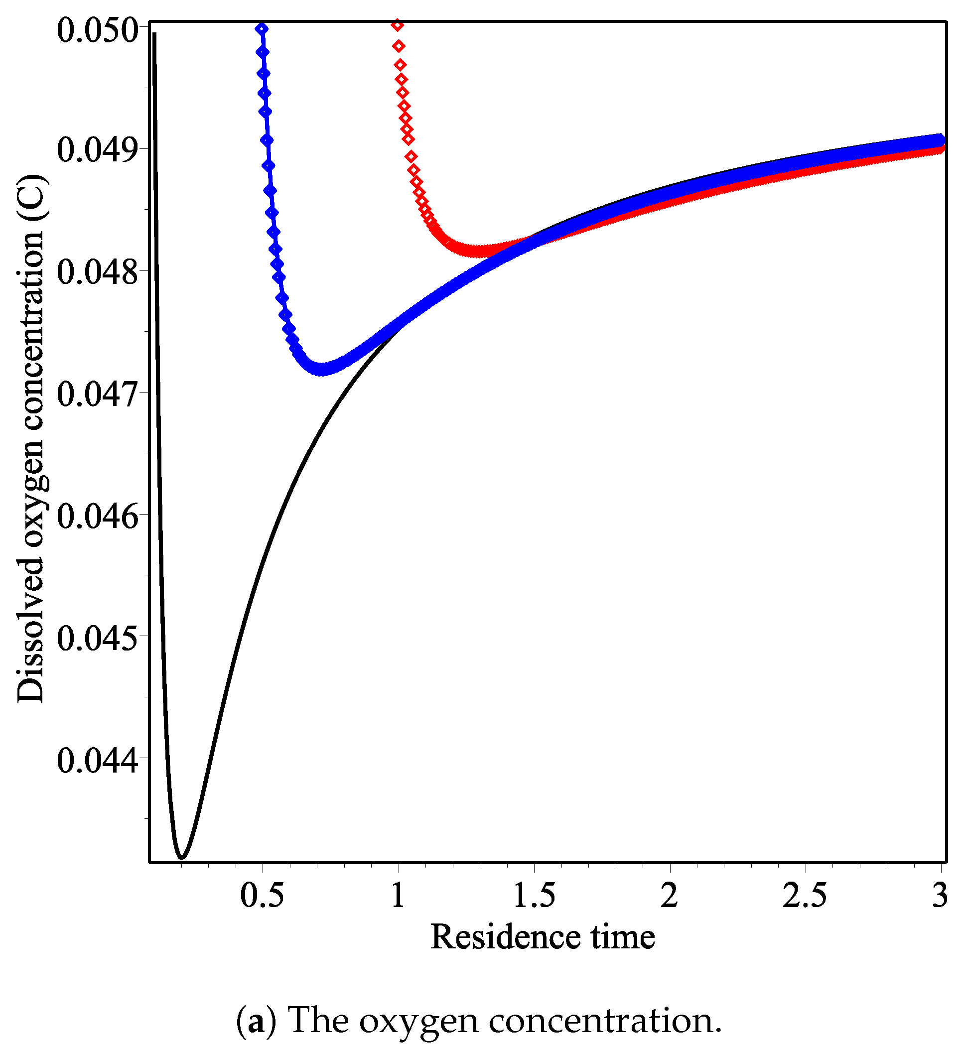
. Figure 1 shows stable curves of the oxygen concentration, the substrate concentration, and the microorganism concentration as functions of residence time for different values of the parameter $\beta$. Note that the parameter $\beta$ represents the configuration of the reactor. $\beta =1$ corresponds to the continuous flow reactor, while $\beta =0$ corresponds to the membrane reactor.

Figure 1a shows that the oxygen concentration decreases as a function of residence time to minimum value, called the minimum residence time. After this minimum value, the oxygen concentration increases as the value of the residence time increases. Note that the minimum residence time for $\beta =1$ and $\beta =0.1$ are 1.30025 and 0.201052, respectively. Thus, the value of parameter $\beta$ must be taken lower to minimise the oxygen concentration.

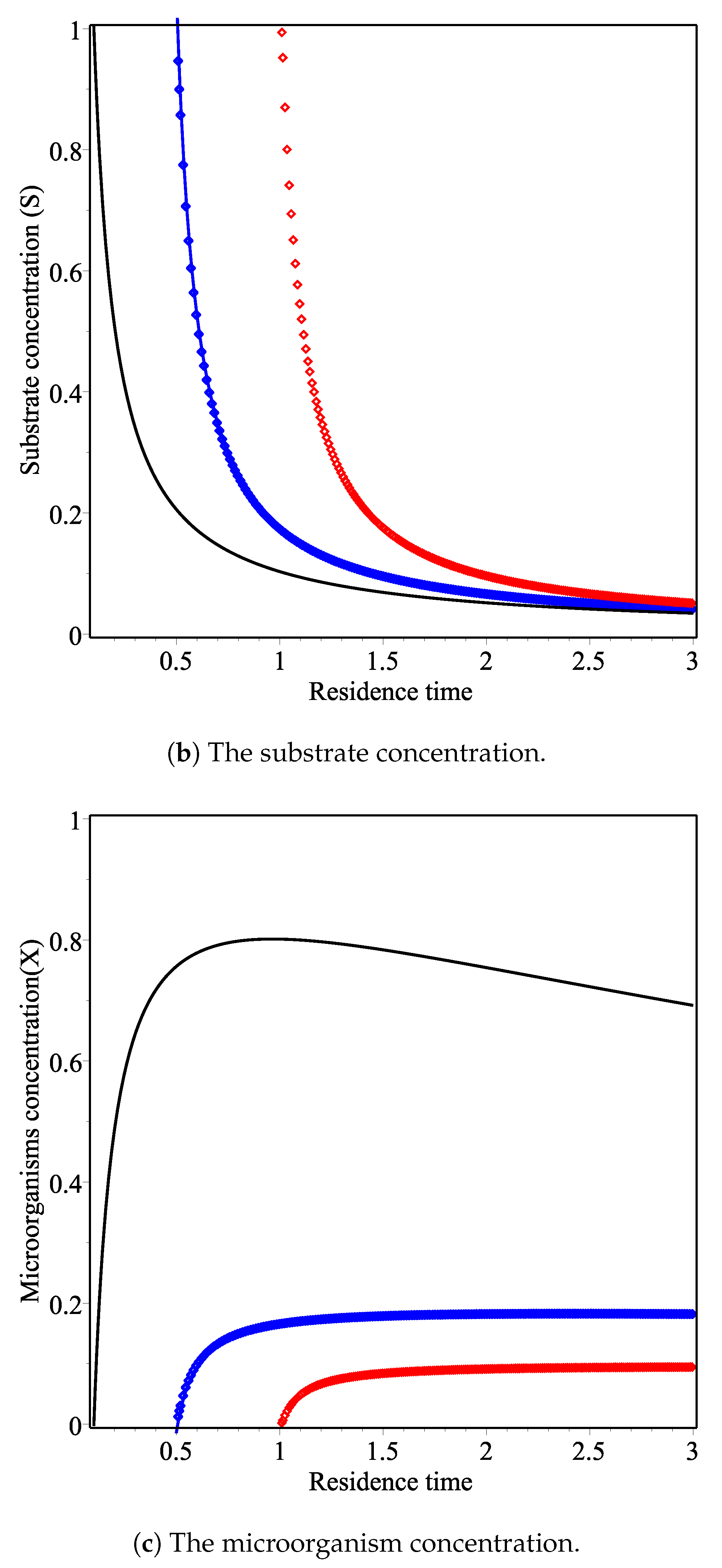
In Figure 1b, the substrate concentration decreases as the value of the residence time increases for different values of $\beta$. In Figure 1c, the microorganism concentration increases to the maximum value, then decreases as the value of the residence time.

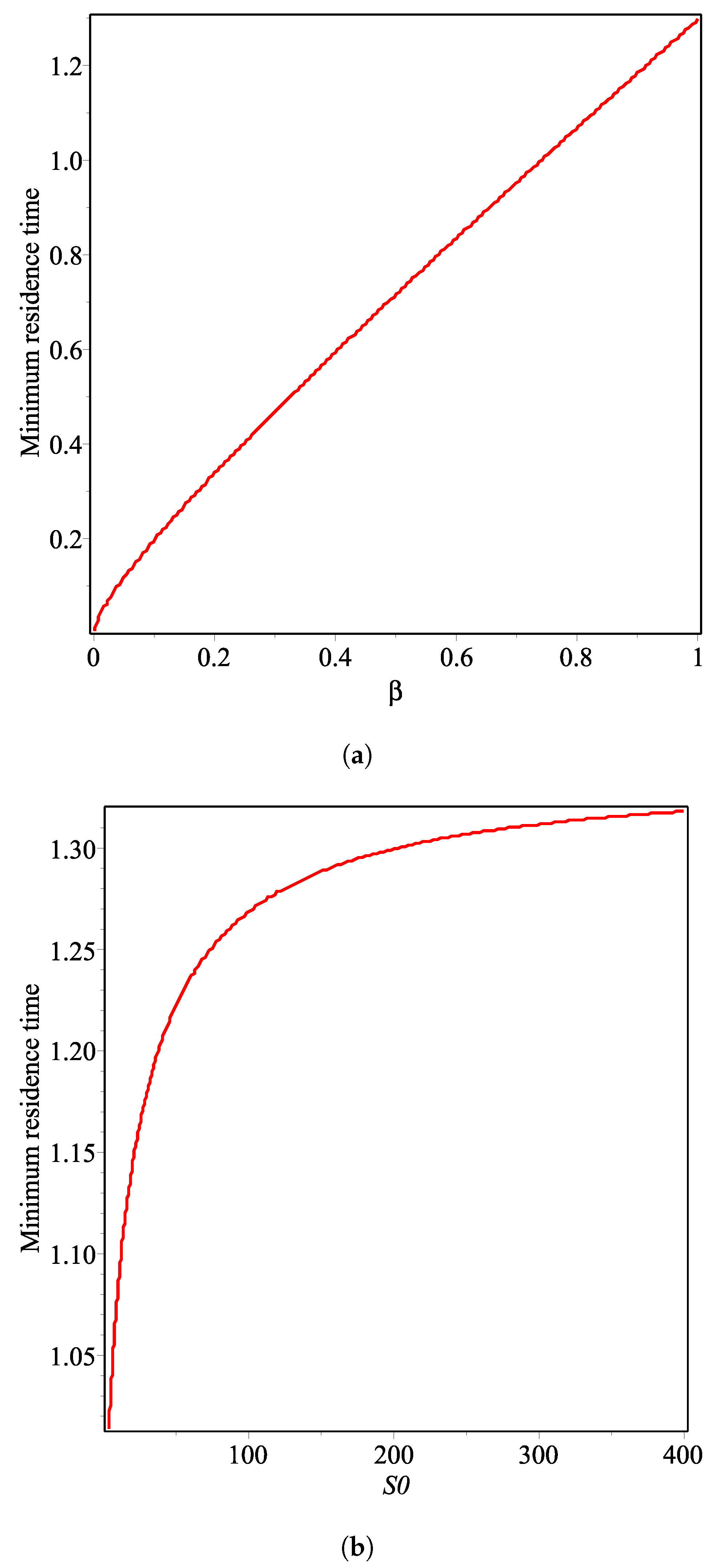
Figure 2 is an unfolding diagram for the minimum residence time in Figure 1a as a function of $\beta$ and the influent concentration ($S_0$). We note that the minimum residence time increases as the value of these parameters increases.

4. Analysis of the Model under Caputo Fractional Operator

Here, we aim to extend the model (4) by incorporating the fractional order in the sense of a Caputor fractional derivative. The model (4) in the sense of a Caputo fractional operator is given by

$$\begin{array}{cc}\hfill {}_{\mathcal{C}}{\mathcal{D}}^{\psi }S& =\frac{1}{{\tau }^{\psi }}(1-S)-\frac{SX}{{\alpha }^{\psi }(S+X)},\hfill \\ \hfill {}_{\mathcal{C}}{\mathcal{D}}^{\psi }X& =\frac{-{\beta }^{\psi }X}{\tau \psi }+\frac{SX}{(S+X)}-K_d^{\psi }X,\hfill \\ \hfill {}_{\mathcal{C}}{\mathcal{D}}^{\psi }C& =\frac{-{\beta }^{\psi }C}{{\tau }^{\psi }}+K_{Ia}^{\psi }(C_0^{\psi }-C)-\frac{SX}{{\gamma }^{\psi }(S+X)}.\hfill \end{array}$$

(13)

4.1. Results for Existence of Solutions under Caputo

In this chapter, we address the existence and uniqueness of the suggested model’s solution via fixed-point theorems. Let’s reformulate the proposed (13) model in the form below:

$$\left\{\begin{array}{cc}{}^C{\mathcal{D}}_{0^{+}}^{\psi }S={\zeta }_1(t,S,X,C),\hfill & \\ {}^C{\mathcal{D}}_{0^{+}}^{\psi }X={\zeta }_2(t,S,X,C),\hfill \\ {}^C{\mathcal{D}}_{0^{+}}^{\psi }C={\zeta }_3(t,S,X,C),\hfill \end{array}\right.$$

(14)

with

$$\left\{\begin{array}{c}{\zeta }_1(t,S,X,C)=\frac{1}{\tau }(1-S)-\frac{SX}{\alpha (S+X)},\hfill \\ {\zeta }_2(t,S,X,C)=-\frac{\beta X}{\tau }+\frac{SX}{(S+X)}-K_{d}X,\hfill \\ {\zeta }_3(t,S,X,C)=-\frac{\beta C}{\tau }+K_{Ia}(C_0-C)-\frac{SX}{\gamma (S+X)}.\hfill \end{array}\right.$$

(15)

Now, (13) becomes

$$\left\{\begin{array}{cc}{}^C{\mathcal{D}}_0^{\psi }\varpi \left(t\right)=\mathsf{\Lambda }(t,\varpi \left(t\right));t\in J=[0,b],0<\alpha \le 1,\hfill & \\ \varpi \left(0\right)={\varpi }_0\ge 0,\hfill \end{array}\right.$$

(16)

only if

$$\left\{\begin{array}{cc}\varpi \left(t\right)={(S,X,C)}^T,\hfill & \\ \varpi \left(0\right)={(S_0,X_0,C_0)}^T,\hfill \\ \mathsf{\Lambda }(t,\varpi \left(t\right))={\left({\zeta }_i(t,S,X,C)\right)}^T,i=1,2,3,\hfill \end{array}\right.$$

(17)

${(·)}^T$ implies the transpose operation. Now, (16) becomes

$$\begin{array}{cc}\hfill \varpi \left(t\right)& ={\varpi }_0+{\mathcal{J}}_{0^{+}}^{\upsilon }\mathsf{\Lambda }(t,\varpi \left(t\right))\hfill \\ \hfill & ={\varpi }_0+\frac{1}{\mathsf{\Gamma }\left(\upsilon \right)}{\int }_0^t{(t-\tau )}^{\upsilon -1}\mathsf{\Lambda }(\tau ,\varpi \left(\tau \right))d\tau .\hfill \end{array}$$

(18)

Let $\mathbb{E}=C\left(\right[0,b];\mathbb{R})$ be a Banach space for all the functions which are continuous from $\mathbb{R}\to [0,b]$ with the norm ${\displaystyle \parallel \varpi \parallel =\underset{t\in J}{sup}\left|\varpi \left(t\right)\right|}$.

Theorem 1.

Let the function $\mathsf{\Lambda }\in C\left(\right[J,\mathbb{R}\left]\right)$ and maps of the bounded subset of $J\times {\mathbb{R}}^5$ be compact subsets of $\mathbb{R}$. Further, there is a constant ${\mathcal{L}}_{\mathsf{\Lambda }}>0$ whereby

$\left({\mathit{A}}_1\right)$$|\mathsf{\Lambda }(t,{\varpi }_1\left(t\right))-\mathsf{\Lambda }(t,{\varpi }_2\left(t\right))|\le {\mathcal{L}}_{\mathsf{\Lambda }}|{\varpi }_1\left(t\right)-{\varpi }_2\left(t\right)|;$$\forall t\in J$ and all ${\varpi }_1,{\varpi }_2\in C\left([\mathcal{J},\mathbb{R}]\right)$. Thus, (18), which is equivalent to (13), has a unique solution whenever $\mathsf{\Omega }{\mathcal{L}}_{\mathsf{\Lambda }}<1$, and

$$\mathsf{\Omega }=\frac{b^{\psi }}{\mathsf{\Gamma }(\psi +1)}.$$

Proof. 

Consider that $P:\mathbb{E}\to \mathbb{E}$ is defined by

$$\left(P\varpi \right)\left(t\right)={\varpi }_0+\frac{1}{\mathsf{\Gamma }\left(\psi \right)}{\int }_0^t{(t-\tau )}^{\psi -1}\mathsf{\Lambda }(\tau ,\varpi \left(\tau \right))d\tau .$$

(19)

Now, P is the unique solution of (13) and is well-defined and depicts the fixed-point of P. Consider ${sup}_{t\in J}\parallel \mathsf{\Lambda }(t,0)\parallel =M_1$ and $\kappa \ge \parallel {\varpi }_0\parallel +\mathsf{\Omega }{M}_1$. Now, it suffices to justify $P{\mathbb{H}}_{\kappa }\subset {\mathbb{H}}_{\kappa },$ and ${\mathbb{H}}_{\kappa }=\{\varpi \in \mathbb{E}:\parallel \varpi \parallel \le \kappa \},$ as convex and closed. Thus, each $\varpi \in {\mathbb{H}}_{\kappa }$, we have

$$\begin{array}{cc}\hfill \left|\right(P\varpi \left)\right(t\left)\right|& \le |{\varpi }_0|+\frac{1}{\mathsf{\Gamma }\left(\psi \right)}{\int }_0^t{(t-\tau )}^{\psi -1}\left|\mathsf{\Lambda }(\tau ,\varpi \left(\tau \right))\right|d\tau \hfill \\ \hfill & \le {\varpi }_0+\frac{1}{\mathsf{\Gamma }\left(\psi \right)}{\int }_0^t{(t-\tau )}^{\psi -1}\left[\left|\mathsf{\Lambda }\right(\tau ,\varpi \left(\tau \right))-\mathsf{\Lambda }(\tau ,0\left)\right|+\left|\mathsf{\Lambda }\right(\tau ,0\left)\right|\right]d\tau \hfill \\ \hfill & \le {\varpi }_0+\frac{({\mathcal{L}}_{\mathsf{\Lambda }}\kappa +M_1)}{\mathsf{\Gamma }\left(\psi \right)}{\int }_0^t{(t-\tau )}^{\psi -1}d\tau \hfill \\ \hfill & \le {\varpi }_0+\frac{({\mathcal{L}}_{\mathsf{\Lambda }}\kappa +M_1)}{\mathsf{\Gamma }(\psi +1)}{b}^{\psi }\hfill \\ \hfill & \le {\varpi }_0+\mathsf{\Omega }({\mathcal{L}}_{\mathsf{\Lambda }}\kappa +M_1)\hfill \\ \hfill & \le \kappa .\hfill \end{array}$$

(20)

We justify the results. Further, for ${\varpi }_1,{\varpi }_2\in \mathbb{E}$, one attains

$$\begin{array}{cc}\hfill |\left(P{\varpi }_1\right)\left(t\right)-\left(P{\varpi }_2\right)\left(t\right)|& \le \frac{1}{\mathsf{\Gamma }\left(\psi \right)}{\int }_0^t{(t-\tau )}^{\psi -1}|\mathsf{\Lambda }(\tau ,{\varpi }_1\left(\tau \right))-\mathsf{\Lambda }(\tau ,{\varpi }_2\left(\tau \right))|d\tau \hfill \\ \hfill & \le \frac{{\mathcal{L}}_{\mathsf{\Lambda }}}{\mathsf{\Gamma }\left(\psi \right)}{\int }_0^t{(t-\tau )}^{\psi -1}|{\varpi }_1\left(\tau \right)-{\varpi }_2\left(\tau \right)|d\tau \hfill \\ \hfill & \le \mathsf{\Omega }{\mathcal{L}}_{\mathsf{\Lambda }}|{\varpi }_1\left(t\right)-{\varpi }_2\left(t\right)|.\hfill \end{array}$$

(21)

This justifies that $\parallel \left(P{\varpi }_1\right)-\left(P{\varpi }_2\right)\parallel \le \mathsf{\Omega }{\mathcal{L}}_{\mathsf{\Lambda }}\parallel {\varpi }_1-{\varpi }_2\parallel$. Thus, due to Banach contraction, the unique solution for (13) is reached. □

Now, we go for the existence of (13) solutions by Krasnoselskii’s fixed-point justification.

Lemma 3.

Let$M\ne \varnothing$be a closed, bounded, and convex subset of a Banach Space$\mathbb{E}.$Let two operators that respect the given relation be$P_1,P_2.$

• $P_1{\varpi }_1+P_2{\varpi }_2\in M,$ provided that ${\varpi }_1,{\varpi }_2\in M;$
• $P_1$ is compact and continuous;
• $P_2$ is a contraction mapping.

Then, there is $u\in M$ as far as $u=P_{1}u+P_{2}u.$

Theorem 2.

Surmising $\mathsf{\Lambda }:\mathcal{J}\times {\mathbb{R}}^5\to \mathbb{R}$ is continuous and holds for the condition $\left({\mathit{A}}_1\right).$ Further, let

$\left({\mathit{A}}_2\right)$$\left|\mathsf{\Lambda }(t,\varpi )\right|\le \psi \left(t\right),forall(t,\varpi )\in J\times {\mathbb{R}}^{5}and\psi \in C([0,b],{\mathbb{R}}_{+})$.

Thus, Equation (13) has at least one solution whenever

$${\mathcal{L}}_K\parallel {\varpi }_1\left(t_0\right)-{\varpi }_2\left(t_0\right)\parallel <1.$$

Proof. 

Setting ${\displaystyle \underset{t\in J}{sup}\left|\psi \left(t\right)\right|=\parallel \psi \parallel }$ and $\eta \ge \parallel {\varpi }_0\parallel +\mathsf{\Omega }\parallel \psi \parallel ,$ we consider ${\mathbf{B}}_{\eta }=\{\varpi \in \mathbb{E}:\parallel \varpi \parallel \le \eta \}.$ Assume $P_1,P_2$ operators on ${\mathbf{B}}_{\eta }$ are expressed as

$$\left(P_1\varpi \right)\left(t\right)=\frac{1}{\mathsf{\Gamma }\left(\psi \right)}{\int }_0^t{(t-\tau )}^{\psi -1}\mathsf{\Lambda }(\tau ,\varpi \left(\tau \right))d\tau t\in J,$$

and

$$\left(P_2\varpi \right)\left(t\right)=\varpi \left(t_0\right),t\in J.$$

Now, each ${\varpi }_1,{\varpi }_2\in {\mathbf{B}}_{\eta },$ gives

$$\begin{array}{cc}\hfill \parallel \left(P_1{\varpi }_1\right)\left(t\right)+\left(P_2{\varpi }_2\right)\left(t\right)\parallel & \le \parallel {\varpi }_0\parallel +\frac{1}{\mathsf{\Gamma }\left(\psi \right)}{\int }_0^t{(t-\tau )}^{\psi -1}\parallel \mathsf{\Lambda }(\tau ,{\varpi }_1\left(\tau \right))\parallel d\tau \hfill \\ \hfill & \le \parallel {\varpi }_0\parallel +\mathsf{\Omega }\parallel \psi \parallel \hfill \\ \hfill & \le \eta <\infty .\hfill \end{array}$$

(22)

Thus, $P_1{\varpi }_1+P_2{\varpi }_2\in {\mathbf{B}}_{\eta }.$

Further, the contraction of $P_2$ will be proved.

For $t\in J$ and ${\varpi }_1,{\varpi }_2\in {\mathbf{B}}_{\eta },$ one reaches

$$\parallel \left(P_2{\varpi }_1\right)\left(t\right)-\left(P_2{\varpi }_2\right)\left(t\right)\parallel \le \parallel {\varpi }_1\left(t_0\right)-{\varpi }_2\left(t_0\right)\parallel .$$

(23)

Having $\mathsf{\Lambda }$ as a continuous function, $P_1$ will also be continuous. Moreover, for any $t\in J$ and ${\varpi }_1\in {\mathbf{B}}_{\eta },$

$$\parallel P_1\varpi \parallel \le \mathsf{\Omega }\parallel \psi \parallel <+\infty ,$$

implies that $P_1$ is uniformly bounded. At last, one can justify that $P_1$ is compact. Defining ${\displaystyle \underset{(t,\varpi )\in J\times {\mathbf{B}}_{\eta }}{sup}\left|\mathsf{\Lambda }(t,\varpi \left(t\right))\right|={\mathsf{\Lambda }}^{*},}$ yields

$$\begin{array}{cc}\hfill |\left(P_1\varpi \right)\left(t_2\right)-\left(P_1\varpi \right)\left(t_2\right)|& =\frac{1}{\mathsf{\Gamma }\left(\psi \right)}|{\int }_0^{t_1}[{(t_2-\tau )}^{\psi -1}-{(t_1-\tau )}^{\psi -1}]\mathsf{\Lambda }(\tau ,\varpi \left(\tau \right))d\tau \hfill \\ \hfill & +{\int }_{t_1}^{t_2}{(t_2-\tau )}^{\psi -1}\mathsf{\Lambda }(\tau ,\varpi \left(\tau \right))d\tau |\hfill \\ \hfill & \le \frac{{\mathsf{\Lambda }}^{*}}{\mathsf{\Gamma }\left(\psi \right)}\left[2{(t_2-t_1)}^{\psi }+(t_2^{\psi }-t_1^{\psi })\right]\hfill \\ \hfill & \to 0,as{t}_2\to t_1.\hfill \end{array}$$

(24)

This shows that by the Arzelá Ascoli principle, (13) has at least one solution. □

4.2. Iterative and Stability Analysis via Caputo Operator

Let $(\mathbb{B},||.|\left|\right)$ be a Banach space and ${\mathbf{Y}}^{*}$ be a self-map of $\mathbb{B}$. Further, consider $y_{n+1}=h({\mathbf{Y}}^{*},y_n)$ and $\mathbf{G}\left({\mathbf{Y}}^{*}\right)$ as a fixed-point set of non-empty ${\mathbf{Y}}^{*}$. It can be interpreted that $y_n$ has converged to $q^{*}\in \mathbf{G}\left({\mathbf{Y}}^{*}\right)$. Defining $\left|\right|z_{n+1}^{*}-h({\mathbf{Y}}^{*},z_n^{*})\left|\right|$ with $\{z_n^{*}\subseteq \mathcal{B}\}$. The iterative scheme, $y_{n+1}=h({\mathbf{Y}}^{*},y_n)$ is ${\mathbf{Y}}^{*}$-stable if ${lim}_{n\to \infty }{c}_n=0$, that is, ${lim}_{n\to \infty }{c}_n^{*}=p^{*}$. To get convergence for $z_n$, it has to possess an upper bound. Having satisfied the aforementioned conditions for $y_{n+1}={\mathbf{Y}}^{*}$ with n representing Picard’s iteration as in [40], then the iteration is ${\mathbf{Y}}^{*}$-stable. Thus:

Theorem 3

([40]). Let $(\mathbb{B},||.|\left|\right)$ be a Banach space and ${\mathbf{Y}}^{*}$ be a self-map on $\mathbb{B}$. Then, for all $x,y\in \mathbb{B}$, the inequality as comes next holds

$$\parallel {\mathbf{Y}}_x^{*}-{\mathbf{Y}}_y^{*}\parallel \le K\parallel x-{\mathbf{Y}}_x^{*}\parallel +k\parallel x-y\parallel ,$$

(25)

with $K\ge 0$, $k\in [0,1)$. If we assume that ${\mathbf{Y}}^{*}$ is Picard ${\mathbf{Y}}^{*}$-stable, we can write

$$\begin{array}{cc}\hfill & S_{n+1}\left(t\right)=S_n\left(t\right)+{\mathcal{L}}^{-1}\left\{\frac{1}{s^{\alpha }}\mathcal{L}\left\{\frac{1}{{\tau }^{\psi }}(1-S_n)-\frac{S_n{X}_n}{{\alpha }^{\psi }(X_n+S_n)}\right\}\right\},\hfill \\ \hfill & X_{n+1}\left(t\right)=X_n\left(t\right)+{\mathcal{L}}^{-1}\left\{\frac{1}{s^{\alpha }}\mathcal{L}\left\{-\frac{{\beta }^{\psi }{X}_n}{{\tau }^{\psi }}+\frac{S_n{X}_n}{(X_n+S_n)}-K_d^{\psi }{X}_n\right\}\right\},\hfill \\ \hfill & C_{n+1}\left(t\right)=C_n\left(t\right)+{\mathcal{L}}^{-1}\left\{\frac{1}{s^{\alpha }}\mathcal{L}\left\{-\frac{{\beta }^{\psi }{C}_n}{{\tau }^{\psi }}+K_{Id}^{\psi }(C_0-C_n)-\frac{S_n{X}_n}{{\gamma }^{\psi }(X_n+S_n)}\right\}\right\}.\hfill \end{array}$$

(26)

Theorem 4.

Let $\mathcal{F}$ be a self-map. Then, it is defined as follows:

$$\begin{array}{cc}\hfill & \mathcal{F}\left[S_n\left(t\right)\right]=S_{n+1}\left(t\right)=S_n\left(t\right)+{\mathcal{L}}^{-1}\left\{\frac{1}{s^{\alpha }}\mathcal{L}\left\{\frac{1}{{\tau }^{\psi }}(1-S_n)-\frac{S_n{X}_n}{{\alpha }^{\psi }(X_n+S_n)}\right\}\right\},\hfill \\ \hfill & \mathcal{F}\left[X_n\left(t\right)\right]=X_{n+1}\left(t\right)=X_n\left(t\right)+{\mathcal{L}}^{-1}\left\{\frac{1}{s^{\alpha }}\mathcal{L}\left\{-\frac{{\beta }^{\psi }{X}_n}{{\tau }^{\psi }}+\frac{S_n{X}_n}{(X_n+S_n)}-K_d^{\psi }{X}_n\right\}\right\},\hfill \\ \hfill & \mathcal{F}\left[C_n\left(t\right)\right]=C_{n+1}\left(t\right)=C_n\left(t\right)+{\mathcal{L}}^{-1}\left\{\frac{1}{s^{\alpha }}\mathcal{L}\left\{-\frac{{\beta }^{\psi }{C}_n}{{\tau }^{\psi }}+K_{Id}^{\psi }(C_0-C_n)-\frac{S_n{X}_n}{{\gamma }^{\psi }(X_n+S_n)}\right\}\right\},\hfill \end{array}$$

(27)

that is $\mathcal{F}$-stable in the space of $L^1(a,b)$, only if

$$\left\{\begin{array}{cc}\hfill & \left(1+\frac{1}{{\tau }^{\psi }}(1-{\kappa }_1\left(\rho \right))-\frac{{\kappa }_1\left(\rho \right){\kappa }_2\left(\rho \right)}{{\alpha }^{\psi }(P+Q)}\right)<1,\hfill \\ \hfill & \left(1-\frac{{\beta }^{\psi }{\kappa }_2\left(\rho \right)}{{\tau }^{\psi }}+\frac{{\kappa }_1\left(\rho \right){\kappa }_2\left(\rho \right)}{(P+Q)}-K_d^{\psi }{\kappa }_2\left(\rho \right)\right)<1,\hfill \\ \hfill & \left(1-\frac{{\beta }^{\psi }{\kappa }_3\left(\rho \right)}{{\tau }^{\psi }}+K_{Id}^{\psi }(C_0-{\kappa }_3\left(\rho \right))-\frac{{\kappa }_1\left(\rho \right){\kappa }_2\left(\rho \right)}{{\gamma }^{\psi }(P+Q)}\right)<1.\hfill \end{array}\right.$$

(28)

Proof. 

Since $\mathcal{F}$ is a fixed point, thus, for each $(m,n)\in \mathbb{N}\times \mathbb{N}$, one attains

$$\begin{array}{cc}\hfill & \mathcal{F}\left[S_n\left(t\right)\right]-\mathcal{F}\left[S_m\left(t\right)\right]=S_{n+1}\left(t\right)=S_n\left(t\right)+{\mathcal{L}}^{-1}\left\{\frac{1}{s^{\alpha }}\mathcal{L}\left\{\frac{1}{{\tau }^{\psi }}(1-S_n)-\frac{S_n{X}_n}{{\alpha }^{\psi }(X_n+S_n)}\right\}\right\}\hfill \\ \hfill & -{\mathcal{L}}^{-1}\left\{\frac{1}{s^{\alpha }}\mathcal{L}\left\{\frac{1}{{\tau }^{\psi }}(1-S_m)-\frac{S_m{X}_m}{{\alpha }^{\psi }(X_m+S_m)}\right\}\right\},\hfill \\ \hfill & \mathcal{F}\left[X_n\left(t\right)\right]-\mathcal{F}\left[X_m\left(t\right)\right]=X_{n+1}\left(t\right)=X_n\left(t\right)+{\mathcal{L}}^{-1}\left\{\frac{1}{s^{\alpha }}\mathcal{L}\left\{-\frac{{\beta }^{\psi }{X}_n}{{\tau }^{\psi }}+\frac{S_n{X}_n}{(X_n+S_n)}-K_d^{\psi }{X}_n\right\}\right\}\hfill \\ \hfill & -{\mathcal{L}}^{-1}\left\{\frac{1}{s^{\alpha }}\mathcal{L}\left\{-\frac{{\beta }^{\psi }{X}_m}{{\tau }^{\psi }}+\frac{S_m{X}_m}{(X_m+S_m)}-K_d^{\psi }{X}_m\right\}\right\},\hfill \\ \hfill & \mathcal{F}\left[C_n\left(t\right)\right]-\mathcal{F}\left[C_m\left(t\right)\right]=C_{n+1}\left(t\right)=C_n\left(t\right)+{\mathcal{L}}^{-1}\left\{\frac{1}{s^{\alpha }}\mathcal{L}\left\{-\frac{{\beta }^{\psi }{C}_n}{{\tau }^{\psi }}+K_{Id}^{\psi }(C_0-C_n)-\frac{S_n{X}_n}{{\gamma }^{\psi }(X_n+S_n)}\right\}\right\}\hfill \\ \hfill & -{\mathcal{L}}^{-1}\left\{\frac{1}{s^{\alpha }}\mathcal{L}\left\{-\frac{{\beta }^{\psi }{C}_m}{{\tau }^{\psi }}+K_{Id}^{\psi }(C_0-C_m)-\frac{S_m{X}_m}{{\gamma }^{\psi }(X_n+S_n)}\right\}\right\}.\hfill \end{array}$$

(29)

Imposing norms on both sides of the first equation in (29), we attain

$$\begin{array}{cc}\hfill \parallel & \mathcal{F}\left(S_n\left(t\right)\right)-\mathcal{F}\left(S_m\left(t\right)\right)\parallel =\parallel S_n\left(t\right)-S_m\left(t\right)\hfill \\ & +{\mathcal{L}}^{-1}\left\{\frac{1}{s^{\alpha }}\mathcal{L}\left\{\frac{1}{{\tau }^{\psi }}(1-S_n)-\frac{S_n{X}_n}{{\alpha }^{\psi }(X_n+S_n)}\right\}\right\}\hfill \\ \hfill & -{\mathcal{L}}^{-1}\left\{\frac{1}{s^{\alpha }}\mathcal{L}\left\{\frac{1}{{\tau }^{\psi }}(1-S_m)-\frac{S_m{X}_m}{{\alpha }^{\psi }(X_m+S_m)}\right\}\right\},\parallel ,\hfill \end{array}$$

(30)

and imposing a triangular inequality gives

$$\begin{array}{cc}\hfill \parallel & \mathcal{F}\left(S_n\left(t\right)\right)-\mathcal{F}\left(S_m\left(t\right)\right)\parallel =\parallel S_n\left(t\right)-S_m\left(t\right)\parallel \hfill \\ & \parallel +{\mathcal{L}}^{-1}\left\{\frac{1}{s^{\alpha }}\mathcal{L}\left\{\frac{1}{{\tau }^{\psi }}(1-S_n)-\frac{S_n{X}_n}{{\alpha }^{\psi }(X_n+S_n)}\right\}\right\}\hfill \\ \hfill & -{\mathcal{L}}^{-1}\left\{\frac{1}{s^{\alpha }}\mathcal{L}\left\{\frac{1}{{\tau }^{\psi }}(1-S_m)-\frac{S_m{X}_m}{{\alpha }^{\psi }(X_m+S_m)}\right\}\right\},\parallel .\hfill \end{array}$$

(31)

Thus, (31) becomes

$$\begin{array}{cc}\hfill \parallel & \mathcal{F}\left(S_n\left(t\right)\right)-\mathcal{F}\left(S_m\left(t\right)\right)\parallel \le \parallel S_n\left(t\right)-S_m\left(t\right)\parallel \hfill \\ & +{\mathcal{L}}^{-1}\left\{\frac{1}{s^{\alpha }}\mathcal{L}\left\{\parallel \frac{1}{{\tau }^{\psi }}(1-S_n)\parallel -\parallel \frac{S_n{X}_n}{{\alpha }^{\psi }(X_n+S_n)}\parallel \right\}\right\}\hfill \\ \hfill & -{\mathcal{L}}^{-1}\left\{\frac{1}{s^{\alpha }}\mathcal{L}\left\{\parallel \frac{1}{{\tau }^{\psi }}(1-S_m)\parallel -\parallel \frac{S_m{X}_m}{{\alpha }^{\psi }(X_m+S_m)}\parallel \right\}\right\}.\hfill \end{array}$$

(32)

To achieve our goal, we assume that

$$\begin{array}{cc}& \parallel X_n\left(t\right)-X_m\left(t\right)\parallel \cong \parallel S_n\left(t\right)-S_m\left(t\right)\parallel ,\hfill \\ & \parallel C_n\left(t\right)-C_m\left(t\right)\parallel \cong \parallel S_n\left(t\right)-S_m\left(t\right)\parallel .\hfill \end{array}$$

(33)

Inserting (33) into the relation (32), one can have

$$\begin{array}{cc}\hfill \parallel & \mathcal{F}\left(S_n\left(t\right)\right)-\mathcal{F}\left(S_m\left(t\right)\right)\parallel \le \parallel S_n\left(t\right)-S_m\left(t\right)\parallel \hfill \\ & +{\mathcal{L}}^{-1}\left\{\frac{1}{s^{\alpha }}\mathcal{L}\left\{\parallel \frac{1}{{\tau }^{\psi }}(1-S_n)\parallel -\parallel \frac{S_n{X}_n}{{\alpha }^{\psi }(X_n+S_n)}\parallel \right\}\right\}\hfill \\ \hfill & -{\mathcal{L}}^{-1}\left\{\frac{1}{s^{\alpha }}\mathcal{L}\left\{\parallel \frac{1}{{\tau }^{\psi }}(1-S_m)\parallel -\parallel \frac{S_m{X}_m}{{\alpha }^{\psi }(X_m+S_m)}\parallel \right\}\right\}.\hfill \end{array}$$

(34)

Since $S_m\left(t\right)$, $X_m\left(t\right)$, and $C_m\left(t\right)$ get convergent and bounded, there exists $P>0$, $Q>0$, and $R>0$ for every t. Thereby, we get

$$\begin{array}{cc}& \parallel S_m\left(t\right)\parallel <P,\parallel X_m\left(t\right)\parallel <Q,\parallel C_m\left(t\right)\parallel <R,(m,n)\in \mathbb{N}\times \mathbb{N}.\hfill \end{array}$$

(35)

From (34) and (35), one reaches

$$\begin{array}{cc}& \parallel \mathcal{F}\left(S_n\left(t\right)\right)-\mathcal{F}\left(S_m\left(t\right)\right)\parallel \le \left(1+\frac{1}{{\tau }^{\psi }}(1-{\kappa }_1\left(\rho \right))-\frac{{\kappa }_1\left(\rho \right){\kappa }_2\left(\rho \right)}{{\alpha }^{\psi }(P+Q)}\right)\parallel (S_n\left(t\right)-S_m\left(t\right))\parallel ,\hfill \end{array}$$

(36)

with ${\kappa }_1$, ${\kappa }_2$, and ${\kappa }_3$ being acquired functions by the inverse Laplace transform in (34). In a similar way, we achieve

$$\parallel \mathcal{F}\left(Q_n\left(t\right)\right)-\mathcal{F}\left(Q_m\left(t\right)\right)\parallel \le \left(1-\frac{{\beta }^{\psi }{\kappa }_2\left(\rho \right)}{{\tau }^{\psi }}+\frac{{\kappa }_1\left(\rho \right){\kappa }_2\left(\rho \right)}{(P+Q)}-K_d^{\psi }{\kappa }_2\left(\rho \right)\right)\parallel Q_n\left(t\right)-Q_m\left(t\right)\parallel ,$$

(37)

$$\parallel \mathcal{F}\left(E_n\left(t\right)\right)-\mathcal{F}\left(E_m\left(t\right)\right)\parallel \le \left(1-\frac{{\beta }^{\psi }{\kappa }_3\left(\rho \right)}{{\tau }^{\psi }}+K_{Id}^{\psi }(C_0-{\kappa }_3\left(\rho \right))-\frac{{\kappa }_1\left(\rho \right){\kappa }_2\left(\rho \right)}{{\gamma }^{\psi }(P+Q)}\right)\parallel E_n\left(t\right)-E_m\left(t\right)\parallel ,$$

(38)

where the condition (28) is valid. Now, $\mathcal{F}$ has a fixed point. To prove that $\mathcal{F}$ holds for Theorem 3.3, let (37) and (38) hold, and the following relations are satisfied:

$$k=(0,0,0),K=\left\{\begin{array}{cc}\hfill & \left(1+\frac{1}{{\tau }^{\psi }}(1-{\kappa }_1\left(\rho \right))-\frac{{\kappa }_1\left(\rho \right){\kappa }_2\left(\rho \right)}{{\alpha }^{\psi }(P+Q)}\right)<1,\hfill \\ \hfill & \left(1-\frac{{\beta }^{\psi }{\kappa }_2\left(\rho \right)}{{\tau }^{\psi }}+\frac{{\kappa }_1\left(\rho \right){\kappa }_2\left(\rho \right)}{(P+Q)}-K_d^{\psi }{\kappa }_2\left(\rho \right)\right)<1,\hfill \\ \hfill & \left(1-\frac{{\beta }^{\psi }{\kappa }_3\left(\rho \right)}{{\tau }^{\psi }}+K_{Id}^{\psi }(C_0-{\kappa }_3\left(\rho \right))-\frac{{\kappa }_1\left(\rho \right){\kappa }_2\left(\rho \right)}{{\gamma }^{\psi }(P+Q)}\right)<1.\hfill \end{array}\right.$$

(39)

Hence, we reach the intended result. □

4.3. The Solution’s Positiveness

Let us decide the invariant region and indicate that for all $t\ge 0$, all solutions of the model’s fractional system are positive. The main objective is to implement the convenience of the analyzed model solutions by observing whether they join the $\mathsf{{\rm Y}}$ invariant field. Employing the benefits of the fractional derivative of Caputo, we assume that

$$\mathsf{{\rm Y}}=(S,X,C)\in {\mathbb{R}}_{+}^3,{\mathbb{R}}_{+}^3=\{n\in {\mathbb{R}}_{+}^3:n\ge 0\}$$

(40)

is a model solution with positive initial conditions.

Further, $n={(S\left(t\right),X\left(t\right),C\left(t\right))}^T.$ We must also show that on each hyperplane that is bound by the non-negative hyperoctant, the vector field points to $\mathbb{R}{+}^3$. Thus, one can write

$$\begin{array}{cc}\hfill & {}_C{\mathbb{D}}^{\psi }S\left(t\right)=\frac{1}{\tau }(1-S)\ge 0,\hfill \\ \hfill & {}_C{\mathbb{D}}^{\psi }Q\left(t\right)=\frac{SX}{S+X}\ge 0,\hfill \\ \hfill & {}_C{\mathbb{D}}^{\psi }E\left(t\right)=K_{Ia}(C_0-C)\ge 0.\hfill \end{array}$$

(41)

Thus, we give the convenient region as follows:

$$\mathsf{{\rm Y}}=\left\{\right(S,X,C):S\ge 0,X\ge 0,C\ge 0,S+X+C\le 1\}.$$

(42)

Thus, in the $\mathsf{{\rm Y}}$ area, the fractional model is biologically acceptable and mathematically well-defined when $t>0$. In addition, this area is positively invariant, that is, the underlying system’s solutions are positive for all t.

5. Numerical Dynamics

This is where, with the aid of the best-suited parameters as obtained in the table, we present different numerical results for the proposed model by using a fractional differential operator known as the Caputo operator. To serve the purpose of model simulations, a predictor-corrector numerical technique for the fractional type of dynamical systems as implemented and analyzed in [41,42,43] has been used on an effective software called Matlab 2019a. In terms of the Caputo differential operator of order $\psi$, the following form of the Cauchy ordinary differential equation is taken into consideration:

$${}_0^C{D}_t^{\psi }\phi \left(t\right)=\varpi \left(t,\phi \left(t\right)\right),{\phi }^{\left(p\right)}\left(0\right)={\phi }_0^p,0<\psi \le 1,0<t\le \tau ,$$

(43)

with $p=0,1,\dots ,n-1,n=⌈\psi ⌉.$ The Volterra equation version of the Equation (43) becomes:

$$\phi \left(t\right)=\sum _{p=0}^{n-1}{\phi }_0^{\left(p\right)}\frac{t^p}{p!}+\frac{1}{\mathsf{\Gamma }\left(\psi \right)}{\int }_0^t{\left(t-s\right)}^{\psi -1}\varpi \left(s,\phi \left(s\right)\right)ds.$$

(44)

Applying the described predictor-corrector related with the Adam-Bashforth-Moulton solver [42], we assume $h=\tau /N,t_j=jh,$ and $j=0,1,\dots ,N\in {\mathrm{Z}}^{+},$ by taking ${\phi }_j\approx \phi \left(t_j\right),$ with ${\phi }_j$ standing for the approximate solution and $\phi \left(t_j\right)$ for the true one. We can now write

$$\begin{array}{ccc}\hfill S_{k+1}& =& \sum _{j=0}^{k-1}{S}_0^{\left(j\right)}\frac{t_{k+1}^j}{j!}+\frac{h^{\psi }}{\mathsf{\Gamma }\left(\psi +2\right)}\sum _{j=0}^k\left(q_{j,k+1}\right)\left(\frac{1}{\tau }(1-S_j)-\frac{S_j{X}_j}{\alpha (S_j+X_j)}\right)\hfill \\ & & +\frac{h^{\psi }}{\mathsf{\Gamma }\left(\psi +2\right)}\sum _{j=0}^k\left(q_{k+1,k+1}\right)\left(\frac{1}{\tau }(1-S_{k+1}^p)-\frac{S_{k+1}^p{X}_{k+1}^p}{\alpha (S_{k+1}^p+X_{k+1}^p)}\right),\hfill \\ \hfill X_{k+1}& =& \sum _{j=0}^{k-1}{X}_0^{\left(j\right)}\frac{t_{k+1}^j}{j!}+\frac{h^{\psi }}{\mathsf{\Gamma }\left(\psi +2\right)}\sum _{j=0}^k\left(q_{j,k+1}\right)\left(-\frac{\beta X_j}{\tau }+\frac{S_j{X}_j}{(S_j+X_j)}-K_d{X}_j\right)\hfill \\ & & +\frac{h^{\psi }}{\mathsf{\Gamma }\left(\psi +2\right)}\sum _{j=0}^k\left(q_{k+1,k+1}\right)\left(-\frac{\beta X_{k+1}^p}{\tau }+\frac{S_{k+1}^p{X}_{k+1}^p}{(S_{k+1}^p+X_{k+1}^p)}-K_d{X}_{k+1}^p\right),\hfill \\ \hfill C_{k+1}& =& \sum _{j=0}^{k-1}{C}_0^{\left(j\right)}\frac{t_{k+1}^j}{j!}+\frac{h^{\psi }}{\mathsf{\Gamma }\left(\psi +2\right)}\sum _{j=0}^k\left(q_{j,k+1}\right)\left(-\frac{\beta C_j}{\tau }+K_{Ia}(C_0-C_j)-\frac{S_j{X}_j}{\gamma (S_j+X_j)}\right)\hfill \\ & & +\frac{h^{\psi }}{\mathsf{\Gamma }\left(\psi +2\right)}\sum _{j=0}^k\left(q_{k+1,k+1}\right)\left(-\frac{\beta C_{k+1}^p}{\tau }+K_{Ia}(C_0-C_{k+1}^p)-\frac{S_{k+1}^p{X}_{k+1}^p}{\gamma (S_{k+1}^p+X_{k+1}^p)}\right),\hfill \end{array}$$

where

$$q_{j,k+1}=\left\{\begin{array}{c}{k}^{\psi +1}-\left(k-\psi \right){\left(k+1\right)}^{\psi },\mathrm{if}j=0,\hfill \\ {\left(k-j+2\right)}^{\psi +1}+{\left(k-j\right)}^{\psi +1}-2{\left(k-j+1\right)}^{\psi +1},\mathrm{if}1\le j\le k,\hfill \\ 1,\mathrm{if}j=k+1.\hfill \end{array}\right.$$

(45)

Here, $\left(p\right)$ implies the predictor portion and it can be determined as:

$$\begin{array}{ccc}\hfill S_{k+1}& =& \sum _{j=0}^{k-1}{S}_0^{\left(j\right)}\frac{t_{k+1}^j}{j!}+\frac{h^{\psi }}{\mathsf{\Gamma }\left(\psi +2\right)}\sum _{j=0}^k\left(w_{j,k+1}\right)\left(\frac{1}{\tau }(1-S_j)-\frac{S_j{X}_j}{\alpha (S_j+X_j)}\right)\hfill \\ \hfill X_{k+1}& =& \sum _{j=0}^{k-1}{X}_0^{\left(j\right)}\frac{t_{k+1}^j}{j!}+\frac{h^{\psi }}{\mathsf{\Gamma }\left(\psi +2\right)}\sum _{j=0}^k\left(w_{j,k+1}\right)\left(-\frac{\beta X_j}{\tau }+\frac{S_j{X}_j}{(S_j+X_j)}-K_d{X}_j\right)\hfill \\ \hfill C_{k+1}& =& \sum _{j=0}^{k-1}{C}_0^{\left(j\right)}\frac{t_{k+1}^j}{j!}+\frac{h^{\psi }}{\mathsf{\Gamma }\left(\psi +2\right)}\sum _{j=0}^k\left(w_{j,k+1}\right)\left(-\frac{\beta C_j}{\tau }+K_{Ia}(C_0-C_j)-\frac{S_j{X}_j}{\gamma (S_j+X_j)}\right)\hfill \end{array}$$

where

$$w_{j,k+1}={\left(k+1-j\right)}^{\psi }-{\left(k-j\right)}^{\psi }.$$

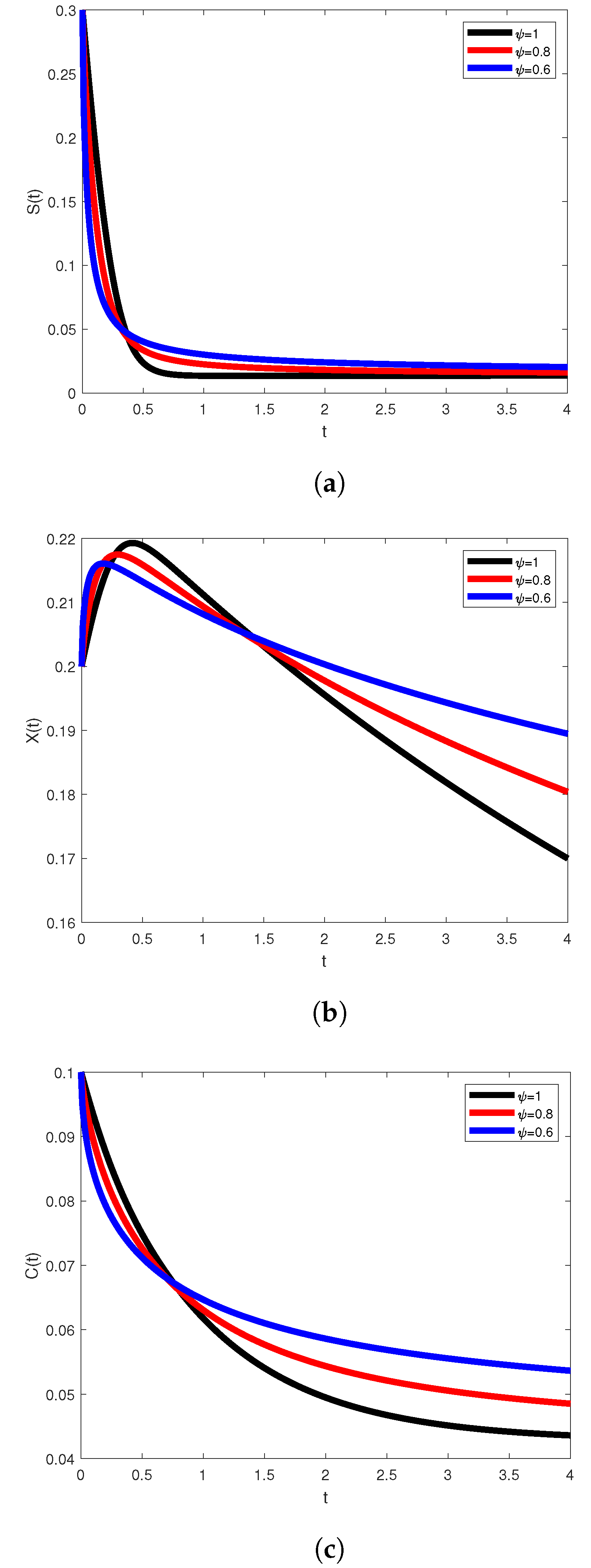
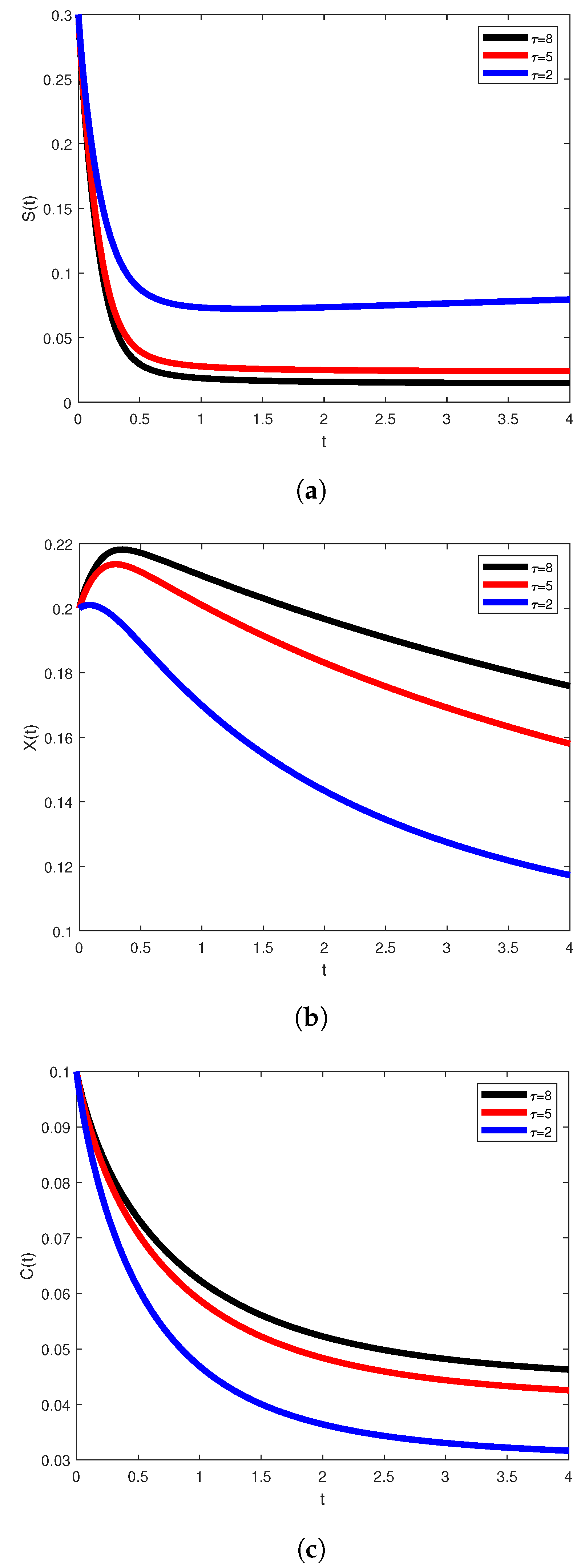
The numerical simulations of the Caputo model (13) using the parameters mentioned in

Table 2. Parameters’ values.

Parameters	Values
$K_d$	0.0140905
$\alpha$	0.10194888
$K_{Ia}$	116.1665
$\gamma$	0.322806
$C_0$	$\frac{1}{20}$
$\beta$	0–1

are presented in this section. In order to solve the nonlinear model shown in Equation (13), we used the predictor-corrector Adams technique and obtained graphical results based on the given parameters values. The concentration of substrate $S\left(t\right)$, of oxygen $C\left(t\right)$, and the microorganism concentration $X\left(t\right)$ are investigated using different values of the fractional order $\psi$ in order to see the dynamical behavior of the Caputo model (13) for all three compartments. It can be observed in Figure 3 that the behaviour of the curves changes as the value of fractional order increases. Moreover, the values of one of the most important and effective parameters in the model, which is the main experimental control parameter $\tau$, have been varied in Figure 4 to practically see its influence in the model. Comparing Figure 3 and Figure 4, the changes in the curves can be noticed as a result of the effect of the main experimental control, $\tau$.

6. Conclusions

In the current analysis, the wastewater model has been studied from a classical viewpoint and modelled by one of the most robust non-local fractional operators, called the Caputo operator. Firstly, some important properties of the model in a classical sense were reported. The dynamical features of the model were depicted through the steady-state region in its classical sense. Since it has been proved in the literature that the fractional operators are especially suitable for studying the dynamical behaviour of real-world problems, it is of vehement importance to analyze more critically the dynamics of the model under consideration with the robust fractional operator called Caputo, and also make some comparisons with the classical variant. The fractionalized order is $\psi$. As a consequence, many important characteristics of the proposed fractional version of the model have been reported, such as the formation of the model, the existence and uniqueness of the solution through the fixed-point theorem, iterative solutions, and the solutions’ positivity. It should be observed that the fractional version of the model under investigation more correctly understands the behavior of the model than the variant of the integer order. This has been done by numerous numerical simulations by using an efficient numerical scheme.

References

- Brauer, F.; Castillo-Chavez, C.; Feng, Z. Mathematical Models in Epidemiology; Springer: New York, NY, USA, 2019. [Google Scholar]
- Qureshi, S.; Yusuf, A. Modeling chickenpox disease with fractional derivatives: From caputo to atangana-baleanu. Chaos Solitons Fractals 2019, 122, 111–118. [Google Scholar] [CrossRef]
- Qureshi, S.; Yusuf, A. Mathematical modeling for the impacts of deforestation on wildlife species using Caputo differential operator. Chaos Solitons Fractals 2019, 126, 32–40. [Google Scholar] [CrossRef]
- Jajarmi, A.; Yusuf, A.; Baleanu, D.; Inc, M. A new fractional HRSV model and its optimal control: A non-singular operator approach. Phys. A 2020, 547, 123860. [Google Scholar] [CrossRef]
- Abdulhameed, M.; Muhammad, M.M.; Gital, A.Y.; Yakubu, D.G.; Khan, I. Effect of fractional derivatives on transient MHD flow and radiative heat transfer in a micro-parallel channel at high zeta potentials. Phys. A 2019, 519, 42–71. [Google Scholar] [CrossRef]
- VDubey, P.; Kumar, R.; Kumar, D. Analytical study of fractional Bratu-type equation arising in electro-spun organic nanofibers elaboration. Phys. A 2019, 521, 762–772. [Google Scholar]
- Chang, A.; Sun, H.; Zhang, Y.; Zheng, C.; Min, F. Spatial fractional Darcy’s law to quantify fluid flow in natural reservoirs. Phys. A 2019, 519, 119–126. [Google Scholar] [CrossRef]
- Goulart, A.G.; Lazo, M.J.; Suarez, J.M.S. A new parameterization for the concentration flux using the fractional calculus to model the dispersion of contaminants in the Planetary Boundary Layer. Phys. A 2019, 518, 38–49. [Google Scholar] [CrossRef]
- Ochoaa, F.G.; Gomez, E.; Santos, V.E.; Merchuk, J.C. Oxygen uptake rate in microbial processes: An overview. Biochem. Eng. J. 2010, 49, 289–307. [Google Scholar] [CrossRef]
- Garcia-Ochoa, F.; Gomez, E.; Santos, V. Oxygen transfer and uptake rates during xanthan gum production. Enzyme Microb. Technol. 2000, 27, 680–690. [Google Scholar] [CrossRef]
- Garcia-Ochoa, F.; Gomez, E. Mass transfer coefficient in stirrer tank reactors for xanthan solutions. Biochem. Eng. J. 1998, 1, 1–10. [Google Scholar] [CrossRef]
- Ho, C.; Oldshue, J.Y. (Eds.) Biotechnology Processes: Scale-Up and Mixing; AIChE: New York, NY, USA, 1987. [Google Scholar]
- Andrew, S.P.S. Gas–liquid mass transfer in microbiological reactors. Trans. IChemE 1982, 60, 3–13. [Google Scholar]
- Aiba, S.; Humphrey, A.E.; Mills, N.F. (Eds.) Biochemical Engineering, 2nd ed.; Academic Press: New York, NY, USA, 1973. [Google Scholar]
- Zou, X.; Hang, H.; Chu, J.; Zhuang, Y.; Zhang, S. Oxygen uptake rate optimization with nitrogen regulation for erythromycin production and scale-up from 50 L to 372 m3 scale. Bioresour. Technol. 2009, 100, 1406–1412. [Google Scholar] [CrossRef] [PubMed]
- Palomares, L.A.; Ramirez, O. The effect of dissolved oxygen tension and the utility of oxygen uptake rate in insect cell culture. Cytotechnology 1996, 22, 225–237. [Google Scholar] [CrossRef] [PubMed]
- Bhattacharya, S.C.; Khai, P.Q. Kinetics of Anaerobic Cowdung Digestion. Energy 1987, 12, 497–500. [Google Scholar] [CrossRef]
- Serhani, M.; Gouze, J.L.; Raissi, N. Dynamical study and robustness of a nonlinear wastewater treatment problem. J. Nonlinear Anal. RWA 2011, 12, 487–500. [Google Scholar] [CrossRef]
- Haandel, A.V.; Lubbe, J.V. Handbook Biological Waste Water Treatment; IWA Publishing: Leidschendam, The Netherlands, 2007. [Google Scholar]
- Alqahtani, T.R.; Nelson, I.M.; Worthy, L.A. Analysis of a chemostat model with variable yield coefficient: Contois kinetics. ANZIAM J. 2012, 53, C155–C171. [Google Scholar] [CrossRef][Green Version]
- Alqahtani, T.R.; Nelson, I.M.; Worthy, L.A. A fundamental analysis of continuous flow bioreactor models with recycle around each reactor governed by Contois kinetics. III. Two and three reactor cascades. Chem. Eng. J. 2012, 183, 422–432. [Google Scholar] [CrossRef]
- Koumboulis, F.N.; Kouvakas, N.D.; King, R.E.; Stathaki, A. Two-stage robust control of substrate concentration for an activated sludge process. ISA Trans. 2008, 47, 267–278. [Google Scholar] [CrossRef]
- Jourani, A.; Serhani, M.; Boutoulout, A. Dynamic and controllability of a nonlinear wastewater treatment problem. J. Appl. Math. Inform. 2012, 30, 883–902. [Google Scholar]
- Khan, K.; Zarin, R.; Khan, A.; Yusuf, A.; Al-Shomrani, M.; Ullah, A. Stability analysis of five-grade Leishmania epidemic model with harmonic mean-type incidence rate. Adv. Differ. Equ. 2021, 86. [Google Scholar] [CrossRef]
- Serhani, M.; Cartigny, P.; Raissi, N. Robust feedback design of wastewater treatment problem. Math. Model. Nat. Phenom. 2009, 4, 1139–1143. [Google Scholar] [CrossRef]
- Haegeman, B.; Lobry, C.; Harmand, J. Modeling bacteria flocculation as density-dependent growth. AIChE J. 2007, 53, 535–539. [Google Scholar] [CrossRef]
- Singh, J.; Kumar, D.; Baleanu, D. On the analysis of fractional diabetes model with exponential law. Adv. Differ. Equ. 2018, 2018, 231. [Google Scholar] [CrossRef]
- Yusuf, A.; Acay, B.; Mustafa, U.T.; Inc, M.; Baleanu, D. Mathematical modeling of pine wilt disease with Caputo fractional operatorChaos. Solitons Fractals 2021, 143, 110569. [Google Scholar] [CrossRef]
- Musa, S.S.; Qureshi, S.; Zhao, S.; Yusuf, A.; Mustapha, U.T.; He, D. Mathematical modeling of COVID-19 epidemic with effect of awareness programs. Infect. Dis. Model. 2021, 6, 448–460. [Google Scholar]
- Baba, I.A.; Yusuf, A.; Al-Shomrani, M. A mathematical model for studying rape and its possible mode of control. Results Phys. 2021, 22, 103917. [Google Scholar] [CrossRef]
- Acay, B.; Inc, M. Fractional modeling of temperature dynamics of a building with singular kernels. Chaos Solitons Fractals 2021, 142, 110482. [Google Scholar] [CrossRef]
- Ahmed, I.; Goufo, E.F.D.; Yusuf, A.; Kumam, P.; Chaipanya, P.; Nonlaopon, K. An epidemic prediction from analysis of a combined HIV-COVID-19 co-infection model via ABC fractional Operator. Alex. Eng. J. 2021, 60, 2979–2995. [Google Scholar] [CrossRef]
- Acay, B.; Bas, E.; Abdeljawad, T. Non-local fractional calculus from different viewpoint generated by truncated M-derivative. J. Comput. Appl. Math. 2020, 366, 112410. [Google Scholar] [CrossRef]
- Kirtphaiboon, S.; Humphries, U.; Khan, A.; Yusuf, A. Model of rice blast disease under tropical climate conditions. Chaos Solitons Fractals 2021, 143, 110530. [Google Scholar] [CrossRef]
- Noeiaghdam, S.; Sidorov, D.N. Caputo-Fabrizio Fractional Derivative to Solve the Fractional Model of Energy Supply-Demand System. Math. Model. Eng. Probl. 2020, 7, 359–367. [Google Scholar] [CrossRef]
- Hu, W.C.; Thayanithy, K.; Forster, C.F. A kinetic study of the anaerobic digestion of ice-cream wastewater. Process. Biochem. 2002, 37, 965–971. [Google Scholar] [CrossRef]
- Fikar, M.; Chachuat, B.; Latifi, M.A. Optimal operation of alternating activated sludge processes. Control Eng. Pract. 2005, 13, 853–861. [Google Scholar] [CrossRef][Green Version]
- Henze, M.; Grady, C.P.L., Jr.; Gujer, W.; Marais, G.V.R.; Matsuo, T. A general model for single-sludge wastewater treatment systems. Water Res. 1987, 21, 505–515. [Google Scholar] [CrossRef]
- Yoon, S.-H.; Lee, S. Critical operational parameters for zero sludge production in biological wastewater treatment processes combined with sludge disintegration. Water Res. 2005, 39, 3738–3754. [Google Scholar] [CrossRef]
- Wang, Z.; Yang, D.; Ma, T.; Sun, N. Stability analysis for nonlinear fractional-order systems based on comparison principle. Nonlinear Dyn. 2014, 75, 387–402. [Google Scholar] [CrossRef]
- Diethelma, K.; Ford, N.J.; Freed, A.D. A Predictor-Corrector Approach for the Numerical Solution of Fractional Differential Equations. Nonlinear Dyn. 2002, 29, 3–22. [Google Scholar] [CrossRef]
- Diethelm, K. An algorithm for the numerical solution of differential equations of fractional order. Electron. Trans. Numer. Anal. 1997, 5, 1–6. [Google Scholar]
- Diethelm, K.; Ford, N.J.; Freed, A.D. Detailed error analysis for a fractional Adams method. Numer. Algorithms 2004, 36, 31–52. [Google Scholar] [CrossRef]