A Unifying Framework for Perturbative Exponential Factorizations

Abstract

We propose a framework where Fer and Wilcox expansions for the solution of differential equations are derived from two particular choices for the initial transformation that seeds the product expansion. In this scheme, intermediate expansions can also be envisaged. Recurrence formulas are developed. A new lower bound for the convergence of the Wilcox expansion is provided, as well as some applications of the results. In particular, two examples are worked out up to a high order of approximation to illustrate the behavior of the Wilcox expansion.

1. Introduction

Linear differential equations of the form

$$\dot{x}\equiv \frac{dx}{dt}=A\left(t\right)x,x\left(0\right)=x_0\in {\mathbb{C}}^d,$$

(1)

with $A\left(t\right)$ a $d\times d$ matrix, whose entries are integrable functions of t, are ever-present in many branches of science, the fundamental evolution equation of Quantum Mechanics, the Schrödinger equation, being a particular case. In consequence, solving Equation (1) is of the greatest importance. In spite of their apparent simplicity, however, they are seldom solvable in terms of elementary functions, and so different procedures have been proposed over the years to render approximate solutions. These are specially useful in the analytical treatment of perturbative problems, such as those arising in the time evolution of quantum systems [1], control theory, or problems where time-ordered products are involved [2]. Among them, exponential perturbative expansions have received a great deal of attention, due to some remarkable properties they possess. In particular, if Equation (1) is defined in a Lie group, the approximations they furnish also evolve in the same Lie group. As a consequence, important qualitative properties of the exact solution are also preserved by the approximations. Thus, if Equation (1) represents the time-dependent Schrödinger equation, then the approximate evolution operator is still unitary, and as a consequence, the total sum of (approximate) transition probabilities is the unity, no matter where the expansion is truncated. There are, in fact, many physical problems (in non-linear mechanics, optical spectroscopy, magnetic resonance, etc.) involving periodic fast-oscillating external fields that are also modeled by Equation (1), with $A\left(t\right)$ periodic. In that case, especially tailored expansions incorporating the well-known Floquet theorem [3], such as the average Hamiltonian theory [4] and the Floquet–Magnus expansion [5,6], have also been proposed.

When dealing with the general problem (1), one of the most widely used exponential approximations corresponds to the Magnus expansion [7]

$$x\left(t\right)={\mathrm{e}}^{\mathsf{\Omega }\left(t\right)}{x}_0,$$

(2)

where $\mathsf{\Omega }$ is an infinite series

$$\mathsf{\Omega }\left(t\right)=\sum _{k=1}^{\infty }{\mathsf{\Omega }}_k\left(t\right)$$

(3)

whose terms are linear combinations of time-ordered integrals of nested commutators of A evaluated at different times (see [8] for a review, including applications to several physical and mathematical problems). What is more interesting for our purposes here is that this expansion can be related with a coordinate transformation $x⟼X$ rendering the original system (1) into the trivial equation

$$\frac{dX}{dt}=0,$$

(4)

with the static solution $X\left(t\right)=X\left(0\right)=x_0$, and that the transformation is given precisely by $x\left(t\right)=exp\left(\mathsf{\Omega }\right(t\left)\right)X\left(t\right)$ [9].

In contrast to the Magnus expansion, the Floquet–Magnus expansion obtains the solution with two exponential transformations when $A\left(t\right)$ is periodic, whereas other exponential perturbative expansions are based on infinite product factorizations of $x\left(t\right)$,

$$x\left(t\right)={\mathrm{e}}^{{\mathsf{\Omega }}_1\left(t\right)}{\mathrm{e}}^{{\mathsf{\Omega }}_2\left(t\right)}\cdots {\mathrm{e}}^{{\mathsf{\Omega }}_n\left(t\right)}\cdots x\left(0\right),$$

(5)

such as those proposed by Fer and Wilcox. In fact, as pointed out in [10], both expansions have a curious history, which is worth describing. It was Fer who proposed the expansion that bears his name in [11], although he never applied it to solve any specific problem. Bellman reviewed this paper in the Mathematical Reviews (MR0104009), and even proposed the expansion as an exercise in [12]. Nevertheless, Wilcox identified it in [1] with an alternative factorization, Equation (5), which was indeed a different and new type of expansion. From them on, their historical trajectories move apart. Thus, Fer expansion was rediscovered by Iserles [13] as a tool for the numerical integration of linear differential equations and later on used in Quantum Mechanics [14] and solid-state nuclear magnetic resonance [15], but also as a Lie-group integrator [16,17,18]. On the other hand, Wilcox expansion has been rediscovered several times in the literature, in particular in [19] in the context of nonlinear control systems, and in [20] as a general tool for approximating the time evolution operator in Quantum Mechanics.

The first goal in this work is to recast both infinite product expansions within a unifying framework. This is done by considering, instead of just one exponential transformation, as in the case of the Magnus expansion, a sequence of such transformations, ${\mathrm{e}}^{{\mathsf{\Omega }}_1\left(t\right)},\dots ,{\mathrm{e}}^{{\mathsf{\Omega }}_k\left(t\right)},\dots$, chosen to satisfy certain requirements. To be more specific, suppose one replaces $A\left(t\right)$ in Equation (1) by $\lambda A\left(t\right)$, where $\lambda >0$ is a parameter. Then, if the transformations are chosen so that each ${\mathsf{\Omega }}_k\left(t\right)$ is proportional to ${\lambda }^k$, we recover the Wilcox expansion, whereas we end up with the Fer expansion when each ${\mathsf{\Omega }}_k\left(t\right)$ is an infinite series in $\lambda$ whose first term is proportional to ${\lambda }^{2^{k-1}}$.

We also show that further alternative descriptions yield new factorizations. This additional degree of freedom can be indeed used to deal better with the features of the matrix $A\left(t\right)$, as in Floquet–Magnus, when $A\left(t\right)$ is periodic.

One might then consider this sequence of linear transformations as a generalization of the concept of picture in Quantum Mechanics when Equation (1) refers to the Schrödinger equation.

Our second goal consists of obtaining, on the basis of this framework, new results concerning Wilcox expansion. Thus, we develop a recursive procedure to obtain every order of approximation in terms of nested commutators, as well as a convergence radius bound. We also establish a formal connection of the Wilcox expansion with the Zassenhaus formula [7,21].

Eventually, the important problem of expanding the exponential $exp(A+\epsilon B)$ for $\epsilon >0$ and A, B, two generic non-commuting operators will be addressed, and two applications of the obtained results.

2. A Sequence of Transformations: The General Case

Given the initial value problem (1), let us consider a linear change in variables $x⟼X_1$ of the form

$$x\left(t\right)={\mathrm{e}}^{{\mathsf{\Omega }}_1\left(t\right)}{X}_1\left(t\right),{\mathsf{\Omega }}_1\left(0\right)=0$$

(6)

transforming the original system into

$$\frac{d{X}_1}{dt}=B_1\left(t\right)X_1.$$

(7)

For the time being, the generator ${\mathsf{\Omega }}_1\left(t\right)$ of the transformation is not specified. Then, $B_1\left(t\right)$ can be expressed in terms of $A\left(t\right)$ and ${\mathsf{\Omega }}_1\left(t\right)$ as follows. First, by inserting Equation (6) into Equation (1), and taking Equation (7) into account, one can obtain

$$\frac{d}{dt}exp\left({\mathsf{\Omega }}_1\right)=A\left(t\right)exp\left({\mathsf{\Omega }}_1\right)-exp\left({\mathsf{\Omega }}_1\right)B_1\left(t\right),$$

(8)

whence

$$B_1\left(t\right)={\mathrm{e}}^{-{\mathsf{\Omega }}_1}A\left(t\right){\mathrm{e}}^{{\mathsf{\Omega }}_1}-{\mathrm{e}}^{-{\mathsf{\Omega }}_1}\frac{d}{dt}{\mathrm{e}}^{{\mathsf{\Omega }}_1}.$$

(9)

The derivative of the matrix exponential can be written as [8]

$$\frac{d}{dt}exp\left({\mathsf{\Omega }}_1\left(t\right)\right)=d{exp}_{{\mathsf{\Omega }}_1\left(t\right)}({\dot{\mathsf{\Omega }}}_1\left(t\right))exp\left({\mathsf{\Omega }}_1\right),$$

(10)

where the symbol $d{exp}_{\mathsf{\Omega }}\left(C\right)$ stands for the (everywhere convergent) power series

$$d{exp}_{\mathsf{\Omega }}\left(C\right)=\sum _{k=0}^{\infty }\frac{1}{(k+1)!}{\mathrm{ad}}_{\mathsf{\Omega }}^k\left(C\right)\equiv \frac{exp\left({\mathrm{ad}}_{\mathsf{\Omega }}\right)-I}{{\mathrm{ad}}_{\mathsf{\Omega }}}\left(C\right).$$

(11)

Here ${\mathrm{ad}}_{\mathsf{\Omega }}^{0}C=C$, ${\mathrm{ad}}_{\mathsf{\Omega }}^{k}C=[\mathsf{\Omega },{\mathrm{ad}}_{\mathsf{\Omega }}^{k-1}C]$, and $[\mathsf{\Omega },C]$ denotes the usual commutator. Therefore

$$B_1\left(t\right)={\mathrm{e}}^{-{\mathsf{\Omega }}_1}\left(A\left(t\right)-d{exp}_{{\mathsf{\Omega }}_1\left(t\right)}({\dot{\mathsf{\Omega }}}_1\left(t\right))\right){\mathrm{e}}^{{\mathsf{\Omega }}_1}\equiv {\mathrm{e}}^{-{\mathrm{ad}}_{{\mathsf{\Omega }}_1}}(B_0-G_1)$$

(12)

where

$$B_0\left(t\right)\equiv A\left(t\right),G_1\left(t\right)\equiv d{exp}_{{\mathsf{\Omega }}_1\left(t\right)}({\dot{\mathsf{\Omega }}}_1\left(t\right))$$

(13)

and

$${\mathrm{e}}^{-{\mathrm{ad}}_{{\mathsf{\Omega }}_1}}F=\sum _{k\ge 0}\frac{{(-1)}^k}{k!}{\mathrm{ad}}_{{\mathsf{\Omega }}_1}^{k}F={\mathrm{e}}^{-{\mathsf{\Omega }}_1}F{\mathrm{e}}^{{\mathsf{\Omega }}_1}.$$

(14)

Of course, nothing prevents us from repeating the whole procedure above and introducing a second transformation to Equation (7) of the form

$$X_1\left(t\right)={\mathrm{e}}^{{\mathsf{\Omega }}_2\left(t\right)}{X}_2\left(t\right),{\mathsf{\Omega }}_2\left(0\right)=0,$$

(15)

so that the new variables verify

$$\frac{d{X}_2}{dt}=B_2\left(t\right)X_2.$$

(16)

In general, for the n-th such linear transformation

$$X_{n-1}\left(t\right)={\mathrm{e}}^{{\mathsf{\Omega }}_n\left(t\right)}{X}_n\left(t\right),{\mathsf{\Omega }}_n\left(0\right)=0$$

(17)

with

$$\frac{d{X}_n}{dt}=B_n\left(t\right)X_n,$$

(18)

one has

$$B_n\left(t\right)={\mathrm{e}}^{-{\mathrm{ad}}_{{\mathsf{\Omega }}_n}}(B_{n-1}-G_n),\mathrm{with}{G}_n\left(t\right)=d{exp}_{{\mathsf{\Omega }}_n\left(t\right)}({\dot{\mathsf{\Omega }}}_n\left(t\right))$$

(19)

so that the solution of Equation (1) is expressed as

$$x\left(t\right)={\mathrm{e}}^{{\mathsf{\Omega }}_1\left(t\right)}{\mathrm{e}}^{{\mathsf{\Omega }}_2\left(t\right)}\cdots {\mathrm{e}}^{{\mathsf{\Omega }}_n\left(t\right)}{X}_n\left(t\right).$$

(20)

Alternatively, we can write $B_n\left(t\right)$ in Equation (19) as follows. Since it is also true that [8]

$$\begin{array}{ccc}\hfill d{exp}_{{\mathsf{\Omega }}_n\left(t\right)}({\dot{\mathsf{\Omega }}}_n\left(t\right))& =& \left(\frac{d}{dt}{\mathrm{e}}^{{\mathsf{\Omega }}_n}\right){\mathrm{e}}^{-{\mathsf{\Omega }}_n}=\left({\int }_0^1{\mathrm{e}}^{x{\mathsf{\Omega }}_n}{\dot{\mathsf{\Omega }}}_n{\mathrm{e}}^{(1-x){\mathsf{\Omega }}_n}dx\right){\mathrm{e}}^{-{\mathsf{\Omega }}_n}\hfill \\ & =& {\int }_0^1{\mathrm{e}}^{x{\mathsf{\Omega }}_n}{\dot{\mathsf{\Omega }}}_n{\mathrm{e}}^{-x{\mathsf{\Omega }}_n}dx,\hfill \end{array}$$

(21)

we have

$$\begin{array}{cc}\hfill B_n=& {\mathrm{e}}^{-{\mathsf{\Omega }}_n}{B}_{n-1}{\mathrm{e}}^{{\mathsf{\Omega }}_n}-{\int }_0^1{\mathrm{e}}^{-u{\mathsf{\Omega }}_n}{\dot{\mathsf{\Omega }}}_n{\mathrm{e}}^{u{\mathsf{\Omega }}_n}du\hfill \\ \hfill =& \sum _{k\ge 0}\frac{{(-1)}^k}{(k+1)!}\left((k+1){\mathrm{ad}}_{{\mathsf{\Omega }}_n}^k{B}_{n-1}-{\mathrm{ad}}_{{\mathsf{\Omega }}_n}^k{\dot{\mathsf{\Omega }}}_n\right),n\ge 1.\hfill \end{array}$$

(22)

The important point is, of course, how to choose $B_n$, or, alternatively, ${\mathsf{\Omega }}_n$, i.e., the specific requirements each transformation has to satisfy in order to be useful to approximately solve Equation (1). There are obviously many possibilities, and in the following we analyze two of them, leading to two different and well-known exponential perturbation factorizations mentioned in the Introduction, namely the Wilcox [1] and Fer [11] expansions.

3. Wilcox Expansion

3.1. Recurrences

Let us introduce the (dummy) parameter $\lambda$ in Equation (1) and replace A with $\lambda A$. This is helpful when collecting coefficients, and at the end we can always take $\lambda =1$.

Since the solution of Equation (1) when A is constant, or more generally when $A\left(t_1\right)A\left(t_2\right)=A\left(t_2\right)A\left(t_1\right)$ for all $t_1\ne t_2$, is $x\left(t\right)=exp({\int }_0^{t}A\left(u\right)du)$, it makes sense to take the generator for the first transformation as

$${\mathsf{\Omega }}_1\left(t\right)={\int }_0^t{B}_0\left(u\right)du=\lambda {\int }_0^{t}A\left(u\right)du\equiv \lambda W_1\left(t\right).$$

(23)

Then, according to Equations (12) and (13), we have

$$C_1\equiv B_0-G_1=\sum _{k\ge 1}{\lambda }^k(b_{0,k}-g_{1,k})$$

(24)

where

$$\begin{array}{cc}\hfill & b_{0,1}=A\left(t\right),b_{0,l}=0,l>1\hfill \\ \hfill & g_{1,1}={\dot{W}}_1,g_{1,l}=\frac{1}{l!}{\mathrm{ad}}_{W_1}^{l-1}{\dot{W}}_1,l>1.\hfill \end{array}$$

(25)

With the choice ${\dot{W}}_1=A\left(t\right)$, it turns out that $B_1$ is a power series in $\lambda$ starting with ${\lambda }^2$,

$$B_1\left(t\right)={\mathrm{e}}^{-{\mathrm{ad}}_{{\mathsf{\Omega }}_1}}(B_0-G_1)={\mathrm{e}}^{-\lambda {\mathrm{ad}}_{W_1}}{C}_1=\sum _{l\ge 2}{\lambda }^l{b}_{1,l},$$

(26)

where

$$b_{1,l}=\sum _{k=0}^{l-2}\frac{{(-1)}^k}{k!}{\mathrm{ad}}_{W_1}^k\left(b_{0,l-k}-g_{1,l-k}\right).$$

(27)

We can analogously choose the second transformation proportional to ${\lambda }^2$, i.e., as ${\mathsf{\Omega }}_2\left(t\right)\equiv {\lambda }^2{W}_2\left(t\right)$ for a given $W_2$ to be determined. Then, a straightforward calculation shows that

$$C_2\equiv B_1-G_2=\sum _{l\ge 2}{\lambda }^l(b_{1,l}-g_{2,l})$$

(28)

with

$$g_{2,2}={\dot{W}}_2,g_{2,2l}=\frac{1}{l!}{\mathrm{ad}}_{W_2}^{l-1}{\dot{W}}_2,g_{2,r}=0,r\ne 2l.$$

(29)

The generator $W_2$ is then obtained by imposing that $b_{1,2}-g_{2,2}=0$ in Equation (28), i.e.,

$$g_{2,2}={\dot{W}}_2=b_{1,2}=b_{0,2}-g_{1,2}=-\frac{1}{2}{\mathrm{ad}}_{W_1}{\dot{W}}_1.$$

(30)

In this way, $B_2\left(t\right)$ is a power series in $\lambda$, starting with ${\lambda }^3$,

$$B_2\left(t\right)={\mathrm{e}}^{-{\lambda }^2{\mathrm{ad}}_{W_2}}{C}_2=\sum _{l\ge 3}{\lambda }^l{b}_{2,l}$$

(31)

with

$$b_{2,l}=\sum _{k=0}^{\left[\right(l-1)/2]-1}\frac{{(-1)}^k}{k!}{\mathrm{ad}}_{W_2}^k\left(b_{1,l-2k}-g_{2,l-2k}\right),$$

(32)

where $[·]$ stands for the integer part of the argument. In general, the n-th transformation ${\mathsf{\Omega }}_n\left(t\right)\equiv {\lambda }^n{W}_n\left(t\right)$ is determined in such a way that the power series of $B_n\left(t\right)$ starts with ${\lambda }^{n+1}$. This can be done as follows: from $B_{n-1}={\sum }_{l\ge n}{\lambda }^l{b}_{n-1,l}$, we compute

$$C_n\equiv B_{n-1}-G_n=\sum _{r=n}^{\infty }{\lambda }^r{c}_{n,r}=\sum _{r=n}^{\infty }{\lambda }^r(b_{n-1,r}-g_{n,r})$$

(33)

with

$$g_{n,r}=\left\{\begin{array}{cc}{\displaystyle \frac{1}{l!}{\mathrm{ad}}_{W_n}^{l-1}{\dot{W}}_n,}\hfill & r=nl\hfill \\ 0,\hfill & r\ne nl\hfill \end{array}\right.l=1,2,\dots$$

(34)

Then, $W_n$ is obtained by taking $b_{n-1,n}-g_{n,n}=0$, i.e.,

$${\dot{W}}_n=b_{n-1,n}$$

(35)

and, finally, $B_n$ is determined as

$$B_n={\mathrm{e}}^{-{\lambda }^n{\mathrm{ad}}_{W_n}}{C}_n=\sum _{l=n+1}^{\infty }{\lambda }^l{b}_{n,l}$$

(36)

with

$$b_{n,l}=\sum _{k=0}^{\left[\frac{l-1}{n}\right]-1}\frac{{(-1)}^k}{k!}{\mathrm{ad}}_{W_n}^k{c}_{n,l-nk}.$$

(37)

Notice that, in view of Equations (34) and (37), Equation (35) simplifies to

$${\dot{W}}_n=b_{n-2,n}\mathrm{for}n\ge 3.$$

(38)

The solution of Equation (1) is expressed, after n such transformations, as

$$x\left(t\right)={\mathrm{e}}^{\lambda W_1\left(t\right)}{\mathrm{e}}^{{\lambda }^2{W}_2\left(t\right)}\cdots {\mathrm{e}}^{{\lambda }^n{W}_n\left(t\right)}{X}_n\left(t\right).$$

(39)

An approximation to the exact solution containing all the dependence up to $\mathcal{O}\left({\lambda }^n\right)$ is obtained by taking $X_n=x_0$ in Equation (39).

In spite of this, the truncated factorization ${\mathrm{e}}^{\lambda W_1\left(t\right)}{\mathrm{e}}^{{\lambda }^2{W}_2\left(t\right)}\cdots {\mathrm{e}}^{{\lambda }^n{W}_n\left(t\right)}$ still shares relevant qualitative properties with the evolution operator, such as orthogonality, unitarity, etc.

Recursion (33)–(38) allows one to construct any generator $W_k$ of the expansion in terms of $W_1,\dots ,W_{k-1}$. For illustration, we next collect the first terms

$$\begin{array}{cc}\hfill & {\dot{W}}_1=A\left(t\right),{\dot{W}}_2=-\frac{1}{2}{\mathrm{ad}}_{W_1}{\dot{W}}_1,{\dot{W}}_3=\frac{1}{3}{\mathrm{ad}}_{W_1}^2{\dot{W}}_1\hfill \\ \hfill & {\dot{W}}_4=-\frac{1}{8}{\mathrm{ad}}_{W_1}^3{\dot{W}}_1-\frac{1}{2}{\mathrm{ad}}_{W_2}{\dot{W}}_2,{\dot{W}}_5=\frac{1}{30}{\mathrm{ad}}_{W_1}^4{\dot{W}}_1-{\mathrm{ad}}_{W_2}{\dot{W}}_3\hfill \end{array}$$

(40)

This is the way the Wilcox expansion is built up.

3.2. Explicit Expressions for $W_n\left(t\right)$

Although the recursive procedure (33)–(38) turns out to be very computationally efficient to construct the exponents $W_n\left(t\right)$ for a given $A\left(t\right)$ in practice, it is clear that much insight about the expansion can be gained if an explicit expression for any $W_n$ can be constructed, thus generalizing the treatment originally done by Wilcox up to $n=4$ [1].

Such an expression could be obtained, in principle, by working out the recurrence (33)–(38), but a more direct approach consists of comparing the Dyson perturbation series of $U\left(t\right)$ [22] in the associated initial value problem

$$\dot{U}=\lambda A\left(t\right)U,U\left(0\right)=I,$$

(41)

i.e.,

$$U\left(t\right)=I+\sum _{n=1}^{\infty }{\lambda }^k{P}_k\left(t\right),\mathrm{with}{P}_k\left(t\right)={\int }_0^{t}d{t}_1\cdots {\int }_0^{t_{k-1}}d{t}_{k}A\left(t_1\right)\cdots A\left(t_k\right)$$

(42)

with the expansion in $\lambda$ of the factorization

$$U\left(t\right)={\mathrm{e}}^{\lambda W_1\left(t\right)}{\mathrm{e}}^{{\lambda }^2{W}_2\left(t\right)}\cdots {\mathrm{e}}^{{\lambda }^n{W}_n\left(t\right)}\cdots .$$

(43)

Thus, for the first terms, one has

$$\begin{array}{cc}\hfill P_1& =W_1,P_2=W_2+{\displaystyle \frac{1}{2}}{W}_1^2,P_3=W_3+W_1{W}_2+\frac{1}{3!}{W}_1^3,\hfill \\ \hfill P_4& =W_4+W_1{W}_3+\frac{1}{2}{W}_1^2{W}_2+{\displaystyle \frac{1}{2}}{W}_2^2+\frac{1}{4!}{W}_1^4.\hfill \end{array}$$

(44)

In general, we can write

$$P_n=\sum _{\genfrac{}{}{0pt}{}{p\left(n\right)}{i_1\le i_2\le \cdots \le i_k}}\frac{1}{r_k!}{W}_{i_1}{W}_{i_2}\cdots W_{i_k},i_1\le i_2\le \cdots \le i_k,$$

(45)

where the sum is extended over the total number of partitions $p\left(n\right)$ of the integer n. We recall that a partition $p\left(n\right)$ of the integer n is an n-tuple $(i_1,i_2,\dots ,i_k)$, such that $i_1+i_2+\cdots +i_k=n$, with ordering $i_1\le i_2\le \cdots \le i_k$. Thus, the seven partitions of $n=5$ with the chosen ordering are $\left(5\right)$, $(1,4)$, $(2,3)$, $(1,1,3)$, $(1,2,2)$, $(1,1,1,2)$ and $(1,1,1,1,1)$. In Equation (45), $r_k$ is the number of repeated indices in the partition considered.

By working out Equation (45), one can invert the relations and express $W_n$ in terms of $P_1,\dots ,P_{n-1}$ for any $n\ge 1$. Thus, one obtains

$$\begin{array}{cc}\hfill W_1& =P_1,W_2=P_2-\frac{1}{2}{P}_1^2,W_3=P_3-P_1{P}_2+\frac{1}{3}{P}_1^3,\hfill \\ \hfill W_4& =P_4-P_1{P}_3+\frac{3}{4}{P}_1^2{P}_2+\frac{1}{4}{P}_2{P}_1^2-\frac{1}{2}{P}_2^2-\frac{1}{4}{P}_1^4.\hfill \end{array}$$

(46)

Notice that $W_n$, $n\ge 2$, is expressed in terms of products of iterated integrals $P_{i_1}\cdots P_{i_j}$. Interestingly, it is possible to express these products as proper time-ordered integrals by using a procedure developed in [23]. If we denote

$$A(i_1{i}_2\dots i_n)\equiv {\int }_0^{t}d{t}_1{\int }_0^{t_1}d{t}_2\cdots {\int }_0^{t_{n-1}}d{t}_{n}A\left(t_{i_1}\right)A\left(t_{i_2}\right)\cdots A\left(t_{t_n}\right),$$

(47)

so that $P_n\left(t\right)=A(12\dots n)$, then

$$\begin{array}{cc}\hfill & W_2=A\left(12\right)-\frac{1}{2}A\left(1\right)·A\left(1\right)\hfill \\ \hfill & W_3=A\left(123\right)-A\left(1\right)·A\left(12\right)+\frac{1}{3}A\left(1\right)·A\left(1\right)·A\left(1\right),\hfill \end{array}$$

(48)

etc. Taking into account Fubini’s theorem,

$${\int }_0^{\alpha }dy{\int }_y^{\alpha }f(x,y)dx={\int }_0^{\alpha }dx{\int }_0^{x}f(x,y)dy,$$

(49)

it is clear that $A\left(1\right)·A\left(1\right)=A\left(12\right)+A\left(21\right)$, and thus

$$W_2=A\left(12\right)-\frac{1}{2}\left(A\left(12\right)+A\left(21\right)\right)=\frac{1}{2}\left(A\left(12\right)-A\left(21\right)\right).$$

(50)

We can proceed analogously with the following products

$$\begin{array}{cc}\hfill & A\left(1\right)·A\left(12\right)=A\left(123\right)+A\left(213\right)+A\left(312\right)\hfill \\ \hfill & A\left(1\right)·A\left(1\right)·A\left(1\right)=A\left(123\right)+A\left(132\right)+A\left(213\right)+A\left(231\right)+A\left(312\right)+A\left(321\right),\hfill \end{array}$$

(51)

so that

$$W_3=\frac{1}{3}A\left(123\right)+\frac{1}{3}A\left(132\right)-\frac{2}{3}A\left(213\right)+\frac{1}{3}A\left(231\right)-\frac{2}{3}A\left(312\right)+\frac{1}{3}A\left(321\right).$$

(52)

Carrying out this argument to any order, we can expand all the products of integrals appearing in $W_n$. As a result, each product is replaced by the sum of all possible permutations of time ordering consistent with the time ordering in the factors of this product [24].

At this point, it is illustrative to consider some examples in detail. Thus, the product $A\left(1\right)·A\left(12\right)$ gives the sum of all permutations of three elements, such that the second index is less than the third one. With respect to $A\left(1\right)·A\left(1\right)·A\left(1\right)$, since there is no special ordering, then all possible permutations have to be taken into account. Finally, for the product $P_1{P}_3$ appearing in $W_4$ one has

$$P_1{P}_3=A\left(1\right)·A\left(123\right)=A\left(4123\right)+A\left(3124\right)+A\left(2134\right)+A\left(1234\right).$$

(53)

Proceeding in a similar way, one can show that any product of iterated integrals can be expressed as a sum of iterated integrals. This property is, in fact, related to a much deeper characterization of the group of permutations [23]. If $\mathfrak{S}Symm$ denotes the graded $\mathbb{Q}$-vector space with the fundamental basis given by the disjoint union of the symmetric groups $S_n$ for all $n\ge 0$, then it is possible to define a product ∗ of permutations and a coproduct $\delta$ in $\mathfrak{S}Symm$, so that there is a one-to-one correspondence between iterated integrals and permutations

$$A\left(\sigma \right)·A\left(\tau \right)=A(\sigma \ast \tau ).$$

(54)

The product ∗ was introduced in [25], and, together with the coproduct $\delta$, endows $\mathfrak{S}Symm$ with a structure of Hopf algebra [26], the so-called Malvenuto–Reutenauer Hopf algebra of permutations [27].

In sum, the general structure of the Wilcox expansion terms therefore reads as

$$W_n=\sum _{k=1}^{n!}{\omega }_k^{\left(n\right)}A\left({\sigma }_k\right),$$

(55)

where the summation extends over all the $n!$ permutations ${\sigma }_k\in S_n$ of $\{1,2,\dots ,n\}$. The weights ${\omega }_k^{\left(n\right)}$ are given by rational numbers that can be determined algorithmically for any n, although the general expression for them is not obvious, in contrast with the Magnus expansion, for which such a closed formula exists [28]. This can be then considered as an open problem.

Moreover, if one is interested in obtaining a compact expression for $W_n$ in terms of independent nested commutators of $A\left(t\right)$, as is done in [1] up to $n=4$; one can use the class of bases proposed by Dragt & Forest in [24] for the Lie algebra generated by the operators $A\left(t_1\right),A\left(t_2\right),\dots ,A\left(t_n\right)$. The same procedure as carried out in [23] for the Magnus expansion can be applied here, so that one obtains the general formula

$$\begin{array}{cc}\hfill & W_n\left(t\right)=\sum _{{\tau }_k}{c}_{{\tau }_k}^{\left(n\right)}{\int }_0^{t}d{t}_1{\int }_0^{t_1}d{t}_2\cdots {\int }_0^{t_{n-1}}d{t}_n\hfill \\ \hfill & [A\left(t_{\tau \left(2\right)}\right),[A\left(t_{\tau \left(3\right)}\right)\cdots [A\left(t_{\tau \left(n\right)}\right),A\left(t_1\right)]\cdots ]].\hfill \end{array}$$

(56)

Here, the sum extends over the $(n-1)!$ permutations ${\tau }_k$ of the elements $\{2,3,\dots ,n\}$ and $c_{{\tau }_k}^{\left(n\right)}$ is a rational number that depends on the particular permutation. For a given permutation, say ${\tau }_k$, its value coincides with the prefactor in Equation (55) of the particular term $A\left({\sigma }_k\right)$, corresponding to the permutation ${\sigma }_k\in S_n$, such that

$$\{{\sigma }_k\left(1\right),{\sigma }_k\left(2\right),\dots ,{\sigma }_k(n-1),{\sigma }_k\left(n\right)\}=\{{\tau }_k\left(2\right),{\tau }_k\left(3\right),\dots ,{\tau }_k\left(n\right),1\}.$$

(57)

Thus, if we denote

$$A[i_1{i}_2\dots i_n]\equiv {\int }_0^{t}d{t}_1{\int }_0^{t_1}d{t}_2\cdots {\int }_0^{t_{n-1}}d{t}_n[A\left(t_{i_1}\right),[A\left(t_{i_2}\right),\cdots [A\left(t_{i_{n-1}}\right),A\left(t_{i_n}\right)]\cdots ]]$$

(58)

we obtain for the first terms

$$\begin{array}{cc}\hfill & W_2=-\frac{1}{2}A\left[21\right],\hfill \\ \hfill & W_3=\frac{1}{3}A\left[231\right]+\frac{1}{3}A\left[321\right],\hfill \\ \hfill & W_4=-\frac{1}{4}A\left[3241\right]-\frac{1}{4}A\left[4231\right]-\frac{1}{4}A\left[4321\right],\hfill \\ \hfill & W_5=-\frac{2}{15}A\left[23451\right]-\frac{2}{15}A\left[23541\right]-\frac{2}{15}A\left[24351\right]-\frac{2}{15}A\left[24531\right]\hfill \\ \hfill & -\frac{2}{15}A\left[25341\right]-\frac{2}{15}A\left[25431\right]+\frac{1}{5}A\left[32451\right]+\frac{1}{5}A\left[32541\right]-\frac{2}{15}A\left[34251\right]\hfill \\ \hfill & -\frac{2}{15}A\left[34521\right]-\frac{2}{15}A\left[35241\right]-\frac{2}{15}A\left[35421\right]+\frac{1}{5}A\left[42351\right]+\frac{1}{5}A\left[42531\right]\hfill \\ \hfill & +\frac{1}{5}A\left[43251\right]+\frac{1}{5}A\left[43521\right]-\frac{2}{15}A\left[45231\right]-\frac{2}{15}A\left[45321\right]+\frac{1}{5}A\left[52341\right]\hfill \\ \hfill & +\frac{1}{5}A\left[52431\right]+\frac{1}{5}A\left[53241\right]+\frac{1}{5}A\left[53421\right]+\frac{1}{5}A\left[54231\right]+\frac{1}{5}A\left[54321\right].\hfill \end{array}$$

(59)

In sum, the general structure of the Wilcox expansion terms via commutators uses the same weights as in Equation (55) and reads

$$W_n=\sum _{k=1}^{(n-1)!}{\phantom{\sum }}^{\prime }{\omega }_k^{\left(n\right)}A\left[{\sigma }_k\right],$$

(60)

where the primed sum requires the rightmost element in the permutation $\sigma \left(k\right)$ to be invariant (as in Equation (56)). This element may be chosen at will and, whatever that value, the permutations are build up with the remaining $n-1$ elements. Different, but equivalent, expressions for $W_n$ in terms of commutators are obtained depending on the value fixed at the rightmost position. We stress once again that, although only the first terms have been collected here for simplicity, the whole procedure is algorithmic in nature and has been implemented in a computer algebra system furnishing to evaluate $W_n\left(t\right)$ explicitly for any n [29]. Note that $W_n\left(t\right)$ involves a linear combination of $(n-1)!$ iterated integrals.

3.3. Convergence of Wilcox Expansion

Recursion (33)–(38) is also very useful to provide estimates for the radius of convergence of the Wilcox expansion when Equation (1) is defined in a Banach algebra $\mathcal{A}$, i.e., an algebra that is also a complete normed linear space with a sub-multiplicative norm,

$$\parallel XY\parallel \le \parallel X\parallel \parallel Y\parallel .$$

(61)

If this is the case, then $\parallel {\mathrm{ad}}_{X}Y\parallel \le 2\parallel X\parallel \parallel Y\parallel$ and, in general, $\parallel {\mathrm{ad}}_X^{n}Y\parallel \le 2^n{\parallel X\parallel }^n\parallel Y\parallel$.

As shown in [30,31], if the series

$$M(\lambda ;t)=\sum _{j=1}^{\infty }{\lambda }^j\parallel W_j\left(t\right)\parallel$$

(62)

has a certain radius of convergence $r_c$ for a given t, then, for $\lambda <r<r_c$, the sequence of functions

$${\mathsf{\Psi }}_n\equiv {\mathrm{e}}^{\lambda W_1\left(t\right)}{\mathrm{e}}^{{\lambda }^2{W}_2\left(t\right)}\cdots {\mathrm{e}}^{{\lambda }^n{W}_n\left(t\right)}$$

(63)

converges uniformly on any compact subset of the ball $B(0,r_c)$. Thus, studying the convergence of the Wilcox expansion reduces analysis of the series $M(\lambda ;t)$ and, in particular, its radius of convergence $r_c$.

Let $k\left(t\right)$ be a function such that $\parallel A\left(t\right)\parallel \le k\left(t\right)$ and denote $K\left(t\right)={\int }_0^{t}k\left(s\right)ds$. Then, clearly

$$\parallel b_{0,1}\parallel \le k\left(t\right);\parallel b_{0,l}\parallel =0,l=2,3,\dots$$

(64)

and

$$\parallel W_1\parallel \le K\left(t\right),\parallel W_2\parallel \le \frac{1}{2}{K}^2\left(t\right).$$

(65)

In general, the following bounds can be established by induction

$$\begin{array}{ccc}\hfill \parallel g_{n,r}\left(t\right)\parallel & \le & {\beta }_{n,r}{K}^{r-1}\left(t\right)k\left(t\right),\hfill \\ \hfill \parallel b_{n,l}\left(t\right)\parallel & \le & {\alpha }_{n,l}{K}^{l-1}\left(t\right)k\left(t\right),n=1,2,\dots ;l>n\hfill \\ \hfill \parallel W_n\left(t\right)\parallel & \le & c_n{K}^n\left(t\right),\hfill \end{array}$$

(66)

where

$$\begin{array}{ccc}\hfill {\alpha }_{0,1}& =& 1;{\alpha }_{0,l}=0,l>1\hfill \\ \hfill {\alpha }_{n,l}& =& \sum _{j=0}^{\left[\frac{l-1}{n}\right]-1}\frac{1}{j!}{2}^j{c}_n^j({\alpha }_{n-1,l-nj}+{\beta }_{n,l-nj})n\ge 1,l>n\hfill \\ \hfill {\beta }_{n,r}& =& \left\{\begin{array}{cc}{\displaystyle \frac{1}{l!}{2}^{l-1}n{c}_n^l,}\hfill & \left[\frac{r}{n}\right]=\frac{r}{n}=l\hfill \\ 0,\hfill & \left[\frac{r}{n}\right]\ne \frac{r}{n}\hfill \end{array}\right.\hfill \\ \hfill c_1& =& 1,c_2=\frac{1}{2},c_n=\frac{1}{n}{\alpha }_{n-2,n},n>2.\hfill \end{array}$$

(67)

It is clear that if the series ${\sum }_{j\ge 1}{c}_j{K}^j\left(t\right)$ converges, so does $M(\lambda =1;t)$. Therefore, a sufficient condition for convergence of the Wilcox expansion is obtained by imposing

$$\underset{n\to \infty }{lim}\frac{c_{n+1}{K}^{n+1}\left(t\right)}{c_n{K}^n\left(t\right)}=K\left(t\right)\underset{n\to \infty }{lim}{D}_n<1,$$

(68)

where

$$D_n\equiv \frac{n}{n+1}\frac{{\alpha }_{n-1,n+1}}{{\alpha }_{n-2,n}}.$$

(69)

We have computed this quantity up to $n=2000$ and then extrapolated to the limit $(1/n)\to 0$. Then $D_n\to D_{\infty }=1.51868$, as seen in Figure 1, and thus the convergence of the Wilcox expansion is ensured at least for values of time t such that

$${\int }_0^t\parallel A\left(s\right)\parallel ds\le K\left(t\right)<{\xi }_W=\frac{1}{D_{\infty }}\approx 0.65846$$

(70)

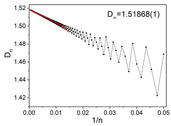
Figure 1. $D_n$ as a function of $1/n$, and linear extrapolation (red line).

This type of extrapolation has also been used to estimate the convergence radius of the Magnus expansion [32]. Although the estimate is not completely analytic, the same type of computation has provided accurate results in other settings. In particular, for the Magnus expansion, such an estimate fully agrees with a purely theoretically deduced bound [8,10,32].

4. Fer–Like Expansions

4.1. Standard Fer Expansion

In forming the Wilcox expansion, the first transformation is chosen in such a way that ${\dot{\mathsf{\Omega }}}_1=B_0\left(t\right)$, whereas ${\dot{\mathsf{\Omega }}}_n\ne B_{n-1}$ for $n\ge 2$. It makes sense, then, to analyze what happens if we impose this condition at each step of the procedure

$${\dot{\mathsf{\Omega }}}_n\left(t\right)=B_{n-1}\left(t\right)\mathrm{or},\mathrm{equivalently},{\mathsf{\Omega }}_n\left(t\right)={\int }_0^t{B}_{n-1}\left(u\right)du$$

(71)

for all $n\ge 1$. In that way, expression (22) for $B_n$ clearly simplifies to

$$B_n\left(t\right)=\sum _{k\ge 1}\frac{{(-1)}^{k}k}{(k+1)!}{\mathrm{ad}}_{{\mathsf{\Omega }}_n}^k{B}_{n-1},n\ge 1.$$

(72)

In doing, so we recover the precise Fer expansion, see [10,11]. Again, after n transformations, we get

$$x\left(t\right)={\mathrm{e}}^{{\mathsf{\Omega }}_1\left(t\right)}{\mathrm{e}}^{{\mathsf{\Omega }}_2\left(t\right)}\cdots {\mathrm{e}}^{{\mathsf{\Omega }}_n\left(t\right)}{X}_n\left(t\right)$$

(73)

so that, if we impose $X_n\left(t\right)=x_0$, we are left with another approximation to the exact solution. Notice that this approximation clearly differs from the previous Wilcox expansion for $n\ge 2$, as can be seen by analyzing the dependence on $\lambda$ of each transformation. Whereas ${\mathsf{\Omega }}_n={\lambda }^n{W}_n\left(t\right)$ for the Wilcox expansion, now ${\mathsf{\Omega }}_n$ contains terms of order ${\lambda }^{2^{n-1}}$ and higher. This can be easily shown by induction: ${\mathsf{\Omega }}_1$ is proportional to $\lambda$, so that $B_1$, according to Equation (72) contains terms of order ${\lambda }^2$ (coming from $[{\mathsf{\Omega }}_1,B_0]$) and higher. In general, $B_{n-2}$ and ${\mathsf{\Omega }}_{n-1}$ contain terms of order ${\lambda }^{2^{n-2}}$ and higher, so the first term in the series (72) for $B_{n-1}$, i.e., the commutator $[{\mathsf{\Omega }}_{n-1},B_{n-2}]$, produces a term of order ${\left({\lambda }^2\right)}^{2^{n-2}}={\lambda }^{2^{n-1}}$ in ${\mathsf{\Omega }}_n$.

Alternatively, expressing Equation (72) as

$$B_n\left(t\right)={\int }_0^{1}dx{\int }_0^{x}du{\mathrm{e}}^{-(1-u){\mathsf{\Omega }}_n}[B_{n-1},{\mathsf{\Omega }}_n]{\mathrm{e}}^{(1-u){\mathsf{\Omega }}_n}$$

(74)

and taking norms, it is then possible to show that the Fer expansion converges for values of t such that [10]

$${\int }_0^t\parallel A\left(s\right)\parallel ds<0.8604065.$$

(75)

4.2. Intermediate Fer-Like Expansions

Notice that the $\lambda$-power series of ${\mathsf{\Omega }}_n$ in the Fer expansion contains infinite terms starting with ${\lambda }^{2^{n-1}}$, but the corresponding truncated factorization obtained from Equation (73) by taking $X_n\left(t\right)=x_0$ is correct only up to terms of order ${\lambda }^{2^{n-1}}$. One might then consider yet another sequence of transformations so that each ${\mathsf{\Omega }}_k$ contains only the relevant terms leading to a correct approximation up to this order. Of course, both factorizations would be different, but nevertheless they would produce the correct power series up to order ${\lambda }^{2^{n-1}}$. The corresponding factorization can be properly called a modified Fer expansion.

Our starting point is, once again, Equation (22). Clearly, the first transformation is the same as in Fer (and Wilcox), i.e.,

$${\dot{\mathsf{\Omega }}}_1=B_0=\lambda A\left(t\right),$$

(76)

and thus

$$B_1=\sum _{k=0}^{\infty }\frac{{(-1)}^{k}k}{(k+1)!}{\mathrm{ad}}_{{\mathsf{\Omega }}_1}^k{B}_0=\mathcal{O}\left({\lambda }^2\right),$$

(77)

where the rightmost term points out the lowest $\lambda$ contribution in the sum.

Next, to reproduce the same dependence on $\lambda$ as the Fer expansion, we need to enforce that $B_2=\mathcal{O}\left({\lambda }^4\right)$, and the question is how to choose ${\mathsf{\Omega }}_2$ guaranteeing this feature. An analysis of Equation (22) with $n=2$ reveals that this is achieved by taking ${\dot{\mathsf{\Omega }}}_2$ as the sum of terms in $B_1$ in Equation (77) contributing to ${\lambda }^2$ and ${\lambda }^3$, i.e.,

$${\dot{\mathsf{\Omega }}}_2=-\frac{1}{2}{\mathrm{ad}}_{{\mathsf{\Omega }}_1}{B}_0+\frac{1}{3}{\mathrm{ad}}_{{\mathsf{\Omega }}_1}^2{B}_0,$$

(78)

since the next term appearing in the expression of $B_2$ involves the computation of ${\mathrm{ad}}_{{\mathsf{\Omega }}_1}^3{B}_0=\mathcal{O}\left({\lambda }^4\right)$. Thus

$$B_2=\sum _{k=1}^{\infty }\frac{{(-1)}^k}{(k+1)!}\left((k+1){\mathrm{ad}}_{{\mathsf{\Omega }}_2}^k{B}_1-{\mathrm{ad}}_{{\mathsf{\Omega }}_2}^k{\dot{\mathsf{\Omega }}}_2\right)=\mathcal{O}\left({\lambda }^4\right).$$

(79)

Likewise, ${\mathsf{\Omega }}_3$ is to be designed so that

$$B_3=\sum _{k=0}^{\infty }\frac{{(-1)}^k}{(k+1)!}\left((k+1){\mathrm{ad}}_{{\mathsf{\Omega }}_3}^k{B}_2-{\mathrm{ad}}_{{\mathsf{\Omega }}_3}^k{\dot{\mathsf{\Omega }}}_3\right)=\mathcal{O}\left({\lambda }^8\right),$$

(80)

and this is guaranteed by taking ${\mathsf{\Omega }}_3$ as the sum all the terms in $B_2$ contributing to powers from ${\lambda }^4$ up to ${\lambda }^7$. From Equation (79) it is clear that

$$B_2=\underset{\mathcal{O}\left({\lambda }^4\right)}{\underbrace{-\frac{1}{2}\left(2{\mathrm{ad}}_{{\mathsf{\Omega }}_2}{B}_1-{\mathrm{ad}}_{{\mathsf{\Omega }}_2}{\dot{\mathsf{\Omega }}}_2\right)}}+\underset{\mathcal{O}\left({\lambda }^6\right)}{\underbrace{\frac{1}{3!}\left(3{\mathrm{ad}}_{{\mathsf{\Omega }}_2}^2{B}_1-{\mathrm{ad}}_{{\mathsf{\Omega }}_2}^2{\dot{\mathsf{\Omega }}}_2\right)}}+\mathcal{O}\left({\lambda }^8\right),$$

(81)

where only the relevant terms in the expansion in $B_1$ have to be taken into account. In this way, we can take

$${\dot{\mathsf{\Omega }}}_3=-{\mathrm{ad}}_{{\mathsf{\Omega }}_2}{B}_1^{\left[4\right]}+\frac{1}{2}{\mathrm{ad}}_{{\mathsf{\Omega }}_2}{\dot{\mathsf{\Omega }}}_2+\frac{1}{2}{\mathrm{ad}}_{{\mathsf{\Omega }}_2}^2{B}_1^{\left[2\right]}-\frac{1}{6}{\mathrm{ad}}_{{\mathsf{\Omega }}_2}^2{\dot{\mathsf{\Omega }}}_2$$

(82)

with

$$B_1^{\left[j\right]}\equiv \sum _{k=1}^j\frac{{(-1)}^k}{(k+1)!}k{\mathrm{ad}}_{{\mathsf{\Omega }}_1}^k{B}_0.$$

(83)

Notice, that since the second term in ${\mathsf{\Omega }}_2$ in Equation (78) is $\mathcal{O}\left({\lambda }^3\right)$, the expression (82) does contain some contributions in ${\lambda }^8$ and ${\lambda }^9$ that in principle could be removed. We prefer, however, to maintain them in order to have a more compact expression.

For this modified Fer expansion, ${\mathsf{\Omega }}_n$ is generally chosen, so that ${\dot{\mathsf{\Omega }}}_n$ is precisely the sum of all terms of $B_{n-1}$ containing terms of powers from ${\lambda }^{2^{n-1}}$ up to ${\lambda }^{2^n-1}$ and then appropriately truncating the series of $B_{n-2},\dots ,B_1$.

Other possibilities for choosing $B_k$ at the successive stages clearly exist, and according to the particular election, different intermediate Fer-like expansions result. In practice, one of those combinations of commutators could be more easily computed for a specific problem.

5. Applications

5.1. Wilcox Expansion as the Continuous Analogue of Zassenhaus Formula

The Zassenhaus formula may be considered as the dual of the Baker–Campbell–Hausdorff (BCH) formula [33] in the sense that it relates the exponential of the sum of two non-commuting operators X and Y with an infinite product of exponentials of these operators and their nested commutators. More specifically,

$${\mathrm{e}}^{X+Y}={\mathrm{e}}^X{\mathrm{e}}^Y\prod _{n=2}^{\infty }{\mathrm{e}}^{C_n(X,Y)}={\mathrm{e}}^X{\mathrm{e}}^Y{\mathrm{e}}^{C_2(X,Y)}{\mathrm{e}}^{C_3(X,Y)}\cdots {\mathrm{e}}^{C_k(X,Y)}\cdots ,$$

(84)

where $C_k(X,Y)$ is a homogeneous Lie polynomial in X and Y of degree k [1,7,21,34,35]. A very efficient procedure to generate all the terms in Equation (84) is presented in [21] and allows to construct $C_n$ up to a prescribed value of n directly, in terms of the minimum number of independent commutators involving n operators X and Y.

In view of the formal similarity between Equations (39) and (84), Wilcox expansion also has been described as the “continuous analogue of the Zassenhaus formula” [10], just as the Magnus expansion is sometimes called the continuous version of the BCH formula. To substantiate this claim, we next reproduce the Zassenhaus Formula (84) by applying the procedure of Section 3 to a particular initial value problem, namely, the abstract equation

$$\dot{U}=\lambda (X+Y)U,U\left(0\right)=I,$$

(85)

where X and Y are two non-commuting constant operators.

The formal solution is, of course, $U\left(t\right)={\mathrm{e}}^{t\lambda (X+Y)}$, but we can also solve Equation (85) by first integrating ${\dot{U}}_0=\lambda X{U}_0$ and factorizing $U\left(t\right)$ as $U\left(t\right)=U_0{U}_I={\mathrm{e}}^{t\lambda X}{U}_I$, where $U_I$ obeys the equation

$${\dot{U}}_I=\lambda {\mathrm{e}}^{-t\lambda X}Y{\mathrm{e}}^{t\lambda X}{U}_I\equiv A_{\lambda }\left(t\right)U_I,$$

(86)

and finally apply this to Equation (86), the sequence of transformations leading to the Wilcox expansion. Notice, however, that now the coefficient matrix $A_{\lambda }\left(t\right)$ is an infinite series in $\lambda$

$$A_{\lambda }\left(t\right)=\lambda {\mathrm{e}}^{-t\lambda {\mathrm{ad}}_X}Y=\sum _{j\ge 0}\frac{{(-1)}^j}{j!}{t}^j{\lambda }^{j+1}{\mathrm{ad}}_X^{j}Y,$$

(87)

so that, when applying the recursion (33)–(38), ${\dot{\mathsf{\Omega }}}_1$ is no longer $B_0\equiv A_{\lambda }\left(t\right)$, but the term in $A_{\lambda }\left(t\right)$ which is proportional to $\lambda$. In other words,

$${\dot{W}}_1=Y,\mathrm{and} \mathrm{thus}{W}_1\left(t\right)=tY.$$

(88)

After some computation, one arrives at

$$b_{0,l}=\frac{{(-1)}^{l-1}}{(l-1)!}{t}^{l-1}{\mathrm{ad}}_X^{l-1}Y.$$

(89)

Since ${\dot{W}}_1=b_{0,1}=Y$, then clearly $g_{1,l}=0$ for all $l>1$ and

$$b_{1,l}=\sum _{k=0}^{l-2}\frac{{(-1)}^k}{k!}{\mathrm{ad}}_{W_1}^k{b}_{0,l-k}.$$

(90)

By imposing $b_{1,2}=g_{2,2}={\dot{W}}_2$, we get

$${\dot{W}}_2=-t{\mathrm{ad}}_{X}Y,\mathrm{so} \mathrm{that}{W}_2\left(t\right)=-\frac{1}{2}{t}^2{\mathrm{ad}}_{X}Y.$$

(91)

In general, $g_{n,n}={\dot{W}}_n$, $g_{n,r}=0$ when $r\ne n$ and the recurrence (33)–(38) reads now

$$\begin{array}{ccc}\hfill {\dot{W}}_1& =& b_{0,1}\hfill \\ \hfill b_{n,l}& =& \sum _{k=0}^{\left[\frac{l-1}{n}\right]-1}\frac{{(-1)}^k}{k!}{\mathrm{ad}}_{W_n}^k{b}_{n-1,l-nk},n=1,2,\dots \hfill \\ \hfill {\dot{W}}_n& =& b_{n-2,n}n\ge 2\hfill \end{array}$$

(92)

together with Equation (89). Working out this recursion we obtain, for the first terms

$$\begin{array}{ccc}\hfill W_3\left(t\right)& =& \frac{1}{6}{t}^3{\mathrm{ad}}_X^{2}Y+\frac{1}{3}{t}^3{\mathrm{ad}}_Y{\mathrm{ad}}_{X}Y\hfill \\ \hfill W_4\left(t\right)& =& -\frac{1}{24}{t}^4{\mathrm{ad}}_X^{3}Y-\frac{1}{8}{t}^4{\mathrm{ad}}_Y{\mathrm{ad}}_X^{2}Y-\frac{1}{8}{t}^4{\mathrm{ad}}_Y^2{\mathrm{ad}}_{X}Y\hfill \\ \hfill W_5\left(t\right)& =& \frac{1}{120}{t}^5{\mathrm{ad}}_X^{4}Y+\frac{1}{30}{t}^5{\mathrm{ad}}_Y{\mathrm{ad}}_X^{3}Y+\frac{1}{20}{t}^5{\mathrm{ad}}_Y^2{\mathrm{ad}}_X^{2}Y\hfill \\ & & +\frac{1}{30}{t}^5{\mathrm{ad}}_Y^3{\mathrm{ad}}_{X}Y+\frac{1}{20}{t}^5{\mathrm{ad}}_{[X,Y]}{\mathrm{ad}}_X^{2}Y+\frac{1}{10}{t}^5{\mathrm{ad}}_{[X,Y]}{\mathrm{ad}}_Y{\mathrm{ad}}_{X}Y\hfill \end{array}$$

(93)

One can see that this procedure agrees with the algorithm presented in [21] for every term $W_n$, $n\ge 1$, in

$$U\left(t\right)={\mathrm{e}}^{t\lambda (X+Y)}={\mathrm{e}}^{t\lambda X}{\mathrm{e}}^{\lambda W_1\left(t\right)}{\mathrm{e}}^{{\lambda }^2{W}_2\left(t\right)}{\mathrm{e}}^{{\lambda }^3{W}_3\left(t\right)}\cdots .$$

(94)

The Zassenhaus formula is recovered by taking $t=1$, i.e., $C_n(X,Y)=W_n(t=1)$.

5.2. Expanding the Exponential $exp(A+\epsilon B)$

Bellman, in his classic book [36], states that “one of the great challenges of modern physics is that of obtaining useful approximate relations for ${\mathrm{e}}^{(A+\epsilon B)t}$ in the case where $AB\ne BA$”. One such approximation was proposed and left undisclosed in ([12], p. 175). Assuming that ${\mathrm{e}}^{A+\epsilon B}$ can be written in the form

$${\mathrm{e}}^{A+\epsilon B}={\mathrm{e}}^A{\mathrm{e}}^{\epsilon C_1}{\mathrm{e}}^{{\epsilon }^2{C}_2}{\mathrm{e}}^{{\epsilon }^3{C}_3}\cdots ,$$

(95)

Bellman proposed to determine the first three terms $C_1$, $C_2$, $C_3$, and pointed out that, contrary to other expansions, the product expansion (95) is unitary if A and B are skew-Hermitian.

It turns out that the Wilcox expansion can be used to provide explicit expressions for $C_n$ for any two indeterminates A and B, as we will see in the sequel.

Before proceeding, it is important to remark that this problem differs from the Zassenhauss formula, in the sense that the expansion parameter affects only one of the operators in the exponential. The solution goes as follows. We write

$$U\left(t\right)\equiv {\mathrm{e}}^{t(A+\epsilon B)}={\mathrm{e}}^{tA}V,$$

(96)

and solve the differential equation satisfied by V

$$\frac{dV}{dt}=\epsilon e^{-tA}B{e}^{tA}V\equiv \epsilon \tilde{B}\left(t\right)V,V\left(0\right)=I$$

(97)

with the Wilcox expansion, so that

$$V\left(t\right)={\mathrm{e}}^{\epsilon W_1\left(t\right)}{\mathrm{e}}^{{\epsilon }^2{W}_2\left(t\right)}{\mathrm{e}}^{{\epsilon }^3{W}_3\left(t\right)}\cdots .$$

(98)

The operators $C_i$ in Equation (95) are then obtained by taking $t=1$.

The successive terms $W_j\left(t\right)$ in Equation (98) can be determined either by the recursion (33)–(38) or the explicit expression (56). For the first term, we get

$$W_1\left(t\right)={\int }_0^t\tilde{B}\left(s\right)dt={\int }_0^t{\mathrm{e}}^{-s{\mathrm{ad}}_A}Bds=\sum _{k=0}^{\infty }\frac{{(-1)}^k{t}^{k+1}}{(k+1)!}{\mathrm{ad}}_A^{k}B$$

(99)

and so the expression for $C_1$ is given by

$$C_1=\frac{1-{\mathrm{e}}^{{\mathrm{ad}}_A}}{{\mathrm{ad}}_A}B=B-\frac{1}{2}[A,B]+\frac{1}{3!}[A,[A,B]]-\frac{1}{4!}[A,[A,[A,B]]]+\cdots .$$

(100)

Although it is possible in principle to construct explicit expressions for $W_2$, $W_3$, etc., it is perhaps more convenient to apply the recursion (33)–(38) for each particular application.

5.3. Illustrative Examples

We next particularize the Bellman problem (95) to matrices where closed expressions for $C_1,C_2,\dots$ can be obtained. The idea is to illustrate the behaviour of the product expansion by computing explicitly high-order terms with matrices in the $\mathrm{SU}\left(2\right)$ and the $\mathrm{SO}\left(3\right)$ Lie algebras.

5.3.1. Matrices X and Y in $\mathrm{SU}\left(2\right)$

In the first example, we chose $A=ia{\sigma }_z$ and $B=i{\sigma }_x$, where $i=\sqrt{-1}$, a is a real parameter and

$${\sigma }_x=\left(\begin{array}{cc}0& 1\\ 1& 0\end{array}\right),{\sigma }_y=\left(\begin{array}{cc}0& -i\\ i& 0\end{array}\right),{\sigma }_z=\left(\begin{array}{cc}1& 0\\ 0& -1\end{array}\right)$$

(101)

are Pauli matrices. This instance is borrowed from Quantum Mechanics, where $exp\left[i(a{\sigma }_z+\epsilon {\sigma }_x)\right]$ is a matrix that transforms the $\frac{1}{2}$-spin wave function in a Hilbert space.

Using the scalar product notation to write down a linear combination of Pauli matrices: $\overrightarrow{v}·\overrightarrow{\sigma }=v_x{\sigma }_x+v_y{\sigma }_y+v_z{\sigma }_z$, the matrix exponential reads

$$exp(i\overrightarrow{v}·\overrightarrow{\sigma })=cosvI+i\frac{sinv}{v}\overrightarrow{v}·\overrightarrow{\sigma }.$$

(102)

In the sequel, we work out the expansion

$${\mathrm{e}}^{i(a{\sigma }_z+\epsilon {\sigma }_x)}={\mathrm{e}}^{ia{\sigma }_z}{\mathrm{e}}^{i\epsilon W_1}{\mathrm{e}}^{i{\epsilon }^2{W}_2}{\mathrm{e}}^{i{\epsilon }^3{W}_3}\dots$$

(103)

up to order eleven in $\epsilon$ and analyze the increasing accuracy of the product expansion as far as more terms are considered. The lhs in Equation (103) may be thought as a transformation involving ${\sigma }_x$ and ${\sigma }_z$. In turn, the rhs is a pure ${\sigma }_z$ transformation, i.e., $exp\left(ia{\sigma }_z\right)$, followed by an infinite succession of transformations, $exp\left(i{\epsilon }^k{W}_k\right)$, whose effect should decrease with k. The truncated product expansion is expected to be accurate as far as $\epsilon \ll a$.

In Table 1 we write down the first five contributions for a generic t (expressions for $k>5$ are too involved to be collected here). Wilcox–Bellman’s Formula (103) corresponds then to $t=1$. All the terms have been obtained with the recurrences of Section 3, starting from

$${\dot{W}}_1\left(t\right)={\mathrm{e}}^{-iat{\sigma }_z}{\sigma }_x{\mathrm{e}}^{iat{\sigma }_z}=C{\sigma }_x+S{\sigma }_y,$$

(104)

where $C\equiv cos\left(2at\right)$ and $S\equiv sin\left(2at\right)$.

Table 1. First five orders in Bellman problem for generic t. The operators $C_k$ in Equation (95) are obtained by taking $t=1$, i.e., $C_k=i{W}_k\left(1\right)$. We have defined $S\equiv sin\left(2at\right)$ and $C\equiv cos\left(2at\right)$.

k	${\mathit{W}}_{\mathit{k}}\left(\mathit{t}\right)$
1	${\displaystyle \frac{1}{2a}}[S{\sigma }_x+(1-C){\sigma }_y]$
2	${\displaystyle \frac{1}{4a^2}}(2at-S){\sigma }_z$
3	${\displaystyle \frac{1}{12a^3}}\left\{[6at+(C-4)S]{\sigma }_x-{(1-C)}^2{\sigma }_y\right\}$
4	$-{\displaystyle \frac{1}{16a^4}}[6at+(C-4)S]{\sigma }_z$
5	${\displaystyle \frac{1}{240a^5}}\left\{[56S-(4C+7)SC-10at(7+4C-2C^2)]{\sigma }_x+\right.$
	$\phantom{{\displaystyle \frac{i}{240a^5}}}\left.[4C^3-7C^2-28C+31+2at(2SC-4S+3at)]{\sigma }_y\right\}$

The formulas in Table 1 show that $\epsilon /a$ may be considered as an effective expansion parameter. In Figure 2, we illustrate, for $a=1$, the accuracy of the Wilcox–Bellman product expansion in the example at hand as a function of $\epsilon$. We plot the squared modulus of the non-diagonal matrix element, say $|U_{1,2}{|}^2$, of Equation (103) for every analytic approximation up to order eleven in $\epsilon$, as well as the exact result. Even orders do not contribute in this test, because $W_{2k}$ is always proportional to ${\sigma }_z$, and therefore $exp\left(i{\epsilon }^{2k}{W}_{2k}\right)$ is a diagonal matrix.

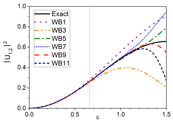
Figure 2. Accuracy of Wilcox–Bellman product expansion up to order eleven as a function of the ratio $\epsilon /a$, with $a=1$. The quantity plotted is the squared modulus of the non-diagonal element of the matrix. The vertical grey line stands for the convergence lower bound $\epsilon =0.658$.Wilcox–Bellman expansion example

As regards convergence of the product expansion, the lower bound of Equation (70) leads to

$${\int }_0^1\parallel {\mathrm{e}}^{-iat{\sigma }_z}\epsilon {\sigma }_x{\mathrm{e}}^{iat{\sigma }_z}\parallel \mathrm{d}t=\epsilon <0.658.$$

(105)

In turn, the behaviour of the curves in Figure 2 points out that convergence of the product expansion extends well beyond that lower bound for this particular example.

Eventually, Figure 3 shows the logarithm of the absolute error in the approximations given by curves in Figure 2.

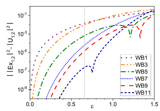
Figure 3. Absolute error of the approximations given by curves in Figure 2 with $a=1$. The vertical grey line is located at the value of the convergence lower bound $\epsilon =0.658$.

5.3.2. Matrices X and Y in $\mathrm{SO}\left(3\right)$

The second example refers to the matrix that describes a rotation in three dimensions defined by the vector $\overrightarrow{a}=\alpha \widehat{a}$. Here, $\alpha$ stands for the rotation angle around the axis given by the unitary vector $\widehat{a}$. A generic 3D rotation matrix can be written as $exp(\overrightarrow{a}·\overrightarrow{\rho })$, where the components of $\overrightarrow{\rho }$ are the three fundamental rotation matrices

$${\rho }_x=\left(\begin{array}{ccc}0& 0& 0\\ 0& 0& -1\\ 0& 1& 0\end{array}\right),{\rho }_y=\left(\begin{array}{ccc}0& 0& 1\\ 0& 0& 0\\ -1& 0& 0\end{array}\right),{\rho }_z=\left(\begin{array}{ccc}0& -1& 0\\ 1& 0& 0\\ 0& 0& 0\end{array}\right).$$

(106)

We study the particular case $\overrightarrow{a}·\overrightarrow{\rho }=\alpha \left(cos\theta {\rho }_z+sin\theta {\rho }_x\right)$, and compare the rotation of angle $\alpha$ around the unit vector $(sin\theta ,0,cos\theta )$

$${\mathrm{e}}^{\alpha \left(cos\theta {\rho }_z+sin\theta {\rho }_x\right)}$$

(107)

with the sequence of transformations

$${\mathrm{e}}^{\alpha cos\theta {\rho }_z}{\mathrm{e}}^{\alpha sin\theta W_1}{\mathrm{e}}^{{(\alpha sin\theta )}^2{W}_2}{\mathrm{e}}^{{(\alpha sin\theta )}^3{W}_3}\dots$$

(108)

In other words, the question we address is how the pure z-axis rotation in Equation (108), $exp(\alpha cos\theta {\rho }_z)$, has to be corrected by an infinite composition of further rotations to reproduce the one defined by $\overrightarrow{a}·\overrightarrow{\rho }$. When $\alpha sin\theta$ is small enough, the approach is expected to converge, since the expansion convergence lower bound reads, in this case, $|\alpha sin\theta |<0.658$.

Here, the accuracy of the product expansion will depend on both the rotation angle $\alpha$ and the relative orientation of the rotation axis, determined by the angle $\theta$. This is illustrated in Figure 4 and Figure 5 for the first five orders of approximation, with $\alpha =\pi /4,\pi /2,3\pi /4$ and $\pi$.

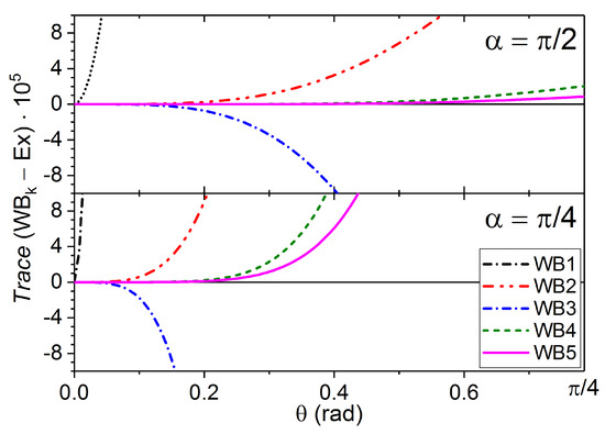
Figure 4. Error in the approximations to the matrix trace as a function of the rotation angle $\theta$, for two values $\alpha =\pi /2$ and $\pi /4$.

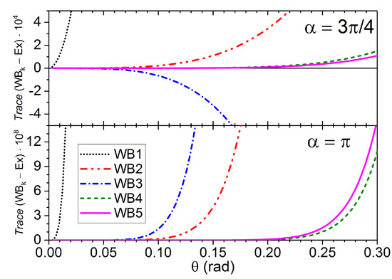
Figure 5. Error in the approximations to the matrix trace as a function of the rotation angle $\theta$, for two values $\alpha =3\pi /4$ and $\pi$.

In order to test the expansion, we have computed the matrix trace of the successive approximants and compared them with the exact result

$$\mathrm{tr}\left(exp\left(\alpha \left(cos\theta {\rho }_z+sin\theta {\rho }_x\right)\right)\right)=1+2cos\alpha .$$

(109)

The first two approximants are simple enough to be written down

$$\begin{array}{cc}\hfill & \mathrm{tr}\left({\mathrm{e}}^{\alpha cos\theta {\rho }_z}{\mathrm{e}}^{\alpha sin\theta W_1}\right)=\left(1+cos(\alpha cos\theta )\right)cos\left(2tan\theta sin\frac{\alpha cos\theta }{2}\right)\hfill \\ \hfill & \mathrm{tr}\left({\mathrm{e}}^{\alpha cos\theta {\rho }_z}{\mathrm{e}}^{\alpha sin\theta W_1}{\mathrm{e}}^{{(\alpha sin\theta )}^2{W}_2}\right)=cos\left(\frac{1}{2}{tan}^2\theta (sin(\alpha cos\theta )-\alpha cos\theta )\right)·\hfill \\ \hfill & \phantom{\mathrm{tr}\left({\mathrm{e}}^{\alpha cos\theta {\rho }_z}{\mathrm{e}}^{\alpha sin\theta W_1}{\mathrm{e}}^{{(\alpha sin\theta )}^2{W}_2}\right)=}cos\left(\alpha cos\theta -\frac{1}{2}tan\theta sin\frac{\alpha cos\theta }{2}\right)\hfill \end{array}$$

(110)

Interestingly, the third approximation order is worse than the second one in all four cases. In the case of $\alpha =\pi$, the fourth order is better than the fifth one.

6. Conclusions

When a linear system of differential equations, defined by the coefficient matrix $\lambda A\left(t\right)$, is transformed under $exp\left(\lambda {\int }_0^{t}A\left(t^{\prime }\right)\mathrm{d}{t}^{\prime }\right)$, the coefficient matrix in the new representation becomes an infinite power series in $\lambda$, say $\tilde{A}\left(t\right)={\sum }_{k\ge 1}{\lambda }^k{a}_k\left(t\right)$. That is the first step of all matrix exponential methods to approximate the time-evolution operator. In the framework that we have introduced, it is the first move in a sequence of exponential transformations that change the linear system from one representation to another with the goal that dynamics will become less and less relevant. Choosing the transformation $exp\left(\lambda {\int }_0^t\tilde{A}\left(x\right)\mathrm{d}x\right)$ as the second move and iterating this procedure afterwards yields the Fer expansion. Instead, choosing the transformation $exp\left(\lambda {\int }_0^t{a}_1\left(x\right)\mathrm{d}x\right)$, i.e., the leading term of the new coefficient matrix, opens up Wilcox expansion. The framework allows for intermediate expansions, taking $exp\left({\sum }_{k=1}^n{\lambda }^k{\int }_0^t{a}_k\left(x\right)\mathrm{d}x\right)$ as an initiator, as well as jumping between schemes, in accordance with the particular requirements of the problem at hand.

We have seen that the theory of linear transformations (or changes of picture in the language of Quantum Mechanics) provides a unified framework to deal with many different exponential perturbative expansions. Whereas only one linear transformation reducing the dynamics to the trivial Equation (4) or to a system with a constant matrix renders the Magnus [9] and the Floquet–Magnus [37] expansion, respectively, a sequence of such transformations with different choices of the new matrices lead to Wilcox and Fer factorizations. From this perspective, other factorizations are possible depending on the particular problem at hand: one only has to appropriately select the successive transformations.

In the case of Wilcox expansion, we have provided an efficient recursive procedure to compute this. In addition, we have developed a method to build up an explicit expression for any $W_n$ in terms of commutators. This is possible by using similar tools, as in the case of the Magnus expansion, namely by relating products of iterated integrals with the structure of the Hopf algebra of permutations, and by using special bases of nested commutators. A sufficient condition for the expansion convergence has also been obtained.

We have presented some application examples of the results about Wilcox expansion. Firstly, we have shown how to obtain Zassenhaus formula from Wilcox expansion which, in turn, may be interpreted as its continuous analogue. Secondly, we point out that Wilcox expansion solves the problem of expanding the exponential $exp(A+ϵB)$ when A and B are non-commuting operators. We refer to this as Wilcox–Bellman expansion. Two practical cases, in this respect, have been analyzed up to high order. Interestingly, in one of them the convergence seems to not be uniform. For convenience, the interested reader can find, in [29], a Mathematica code generating general explicit expressions and recurrences for the Wilcox expansion.

While a full assessment of the Wilcox expansion in comparison with Fer expansion is not the main purpose of this work, we can still mention some of their most distinctive features. Both types of expansion construct the solution of Equation (1) as an infinite exponential factorization, but in Wilcox, the exponent of each factor is proportional to successive powers of the expansion parameter $\lambda$, whereas, in Fer, each exponent contains an infinite sum of powers of $\lambda$. This means that, when truncated after a given number of transformations, say n, the Wilcox expansion differs from the exact solution in the power ${\lambda }^{n+1}$. In other words, each term $W_k\left(t\right)$ in the Wilcox expansion collects the effect of the perturbation at order k. On the other hand, the Fer expansion, when truncated after n transformations, provides a much more accurate approximation. This is true, of course, if the infinite sums involved in each transformation are exactly computed, an almost impossible task unless the time dependence of $A\left(t\right)$ is simple enough. By contrast, we have explicit expressions for each exponent $W_k\left(t\right)$ in the Wilcox expansion for a generic $A\left(t\right)$ and, by using the same techniques as in the Magnus expansion, we can construct appropriate approximations of the iterated integrals if necessary. As the examples collected here and in some other studies show [20], Wilcox expansion can provide accurate results after only a few such transformations.

References

- Wilcox, R. Exponential operators and parameter differentiation in quantum physics. J. Math. Phys. 1967, 8, 962–982. [Google Scholar] [CrossRef]
- Oteo, J.; Ros, J. From time-ordered products to Magnus expansion. J. Math. Phys. 2000, 41, 3268–3277. [Google Scholar] [CrossRef]
- Hale, J. Ordinary Differential Equations; Krieger Publishing Company: Malabar, FL, USA, 1980. [Google Scholar]
- Maricq, M.M. Application of average Hamiltonian theory to the NMR of solids. Phys. Rev. B 1982, 25, 6622–6632. [Google Scholar] [CrossRef]
- Casas, F.; Oteo, J.A.; Ros, J. Floquet theory: Exponential perturbative treatment. J. Phys. A Math. Gen. 2001, 34, 3379–3388. [Google Scholar] [CrossRef]
- Mananga, E.; Charpentier, T. On the Floquet–Magnus expansion: Applications in solid-state nuclear magnetic resonance and physics. Phys. Rep. 2016, 609, 1–50. [Google Scholar] [CrossRef]
- Magnus, W. On the Exponential Solution of Differential Equations for a Linear Operator. Comm. Pure Appl. Math. 1954, VII, 649–673. [Google Scholar] [CrossRef]
- Blanes, S.; Casas, F.; Oteo, J.; Ros, J. The Magnus expansion and some of its applications. Phys. Rep. 2009, 470, 151–238. [Google Scholar] [CrossRef]
- Casas, F.; Chartier, P.; Murua, A. Continuous changes of variables and the Magnus expansion. J. Phys. Commun. 2019, 3, 095014. [Google Scholar] [CrossRef]
- Blanes, S.; Casas, F.; Oteo, J.; Ros, J. Magnus and Fer expansions for matrix differential equations: The convergence problem. J. Phys. A Math. Gen. 1998, 22, 259–268. [Google Scholar] [CrossRef]
- Fer, F. Résolution de l’equation matricielle U˙= pU par produit infini d’exponentielles matricielles. Bull. Classe Sci. Acad. R. Bel. 1958, 44, 818–829. [Google Scholar]
- Bellman, R. Introduction to Matrix Analysis, 2nd ed.; McGraw-Hill: New York, NY, USA, 1970. [Google Scholar]
- Iserles, A. Solving Linear Ordinary Differential Equations by Exponentials of Iterated Commutators. Numer. Math. 1984, 45, 183–199. [Google Scholar] [CrossRef]
- Klarsfeld, S.; Oteo, J. Exponential infinite-product representations of the time displacement operator. J. Phys. A Math. Gen. 1989, 22, 2687–2694. [Google Scholar] [CrossRef]
- Mananga, E. On the Fer expansion: Applications in solid-state nuclear magnetic resonance and physics. Phys. Rep. 2016, 608, 1–41. [Google Scholar] [CrossRef]
- Casas, F. Fer’s Factorization as a Symplectic Integrator. Numer. Math. 1996, 74, 283–303. [Google Scholar] [CrossRef]
- Zanna, A. Collocation and Relaxed Collocation for the Fer and the Magnus Expansions. SIAM J. Numer. Anal. 1999, 36, 1145–1182. [Google Scholar] [CrossRef][Green Version]
- Iserles, A.; Munthe-Kaas, H.; Nørsett, S.; Zanna, A. Lie-Group Methods. Acta Numer. 2000, 9, 215–365. [Google Scholar] [CrossRef]
- Huillet, T.; Monin, A.; Salut, G. Lie algebraic canonical representation in nonlinear control systems. Math. Syst. Theory 1987, 20, 193–213. [Google Scholar] [CrossRef]
- Zagury, N.; Aragão, A.; Casanova, J.; Solano, E. Unitary expansion of the time evolution operator. Phys. Rev. A 2010, 82, 042110. [Google Scholar] [CrossRef]
- Casas, F.; Murua, A.; Nadinic, M. Efficient computation of the Zassenhaus formula. Comput. Phys. Commun. 2012, 183, 2386–2391. [Google Scholar] [CrossRef]
- Galindo, A.; Pascual, P. Quantum Mechanics; Springer: Berlin/Heidelberg, Germany, 1990. [Google Scholar]
- Arnal, A.; Casas, F.; Chiralt, C. A general formula for the Magnus expansion in terms of iterated integrals of right-nested commutators. J. Phys. Commun. 2018, 2, 035024. [Google Scholar] [CrossRef]
- Dragt, A.; Forest, E. Computation of nonlinear behavior of Hamiltonian systems using Lie algebraic methods. J. Math. Phys. 1983, 24, 2734–2744. [Google Scholar] [CrossRef]
- Agrachev, A.; Gamkrelidze, R. The shuffle product and symmetric groups. In Differential Equations, Dynamical Systems, and Control Science; Elworthy, K., Everitt, W., Lee, E., Eds.; Marcel Dekker: New York, NY, USA, 1994; pp. 365–382. [Google Scholar]
- Hazewinkel, M.; Gubareni, N.; Kirichenko, V. Algebras, Rings and Modules. Lie Algebras and Hopf Algebras; AMS: Providence, RI, USA, 2010. [Google Scholar]
- Malvenuto, C.; Reutenauer, C. Duality between quasi-symmetric functions and the Solomon descent algebra. J. Algebra 1995, 177, 967–982. [Google Scholar] [CrossRef]
- Strichartz, R.S. The Campbell–Baker–Hausdorff–Dynkin Formula and Solutions of Differential Equations. J. Funct. Anal. 1987, 72, 320–345. [Google Scholar] [CrossRef]
- Geometric Integration Research Group. 2021. Available online: http://www.gicas.uji.es/Research/Wilcox.html (accessed on 18 February 2021).
- Bayen, F. On the convergence of the Zassenhaus formula. Lett. Math. Phys. 1979, 3, 161–167. [Google Scholar] [CrossRef]
- Arnal, A.; Casas, F.; Chiralt, C. On the structure and convergence of the symmetric Zassenhaus formula. Comput. Phys. Commun. 2017, 217, 58–65. [Google Scholar] [CrossRef]
- Moan, P.; Oteo, J. Convergence of the exponential Lie series. J. Math. Phys. 2001, 42, 501–508. [Google Scholar] [CrossRef]
- Casas, F.; Murua, A. An efficient algorithm for computing the Baker–Campbell–Hausdorff series and some of its applications. J. Math. Phys. 2009, 50, 033513. [Google Scholar] [CrossRef]
- Suzuki, M. On the convergence of exponential operators—The Zassenhaus formula, BCH formula and systematic approximants. Commun. Math. Phys. 1977, 57, 193–200. [Google Scholar] [CrossRef]
- Weyrauch, M.; Scholz, D. Computing the Baker–Campbell–Hausdorff series and the Zassenhaus product. Comput. Phys. Commun. 2009, 180, 1558–1565. [Google Scholar] [CrossRef]
- Bellman, R. Perturbation Techniques in Mathematics, Engineering & Physics; Dover Publications: Mineola, NY, USA, 1972. [Google Scholar]
- Arnal, A.; Casas, F.; Chiralt, C. Exponential perturbative expansions and coordinate transformations. Math. Comput. Appl. 2020, 25, 50. [Google Scholar] [CrossRef]
Publisher’s Note: MDPI stays neutral with regard to jurisdictional claims in published maps and institutional affiliations. |
© 2021 by the authors. Licensee MDPI, Basel, Switzerland. This article is an open access article distributed under the terms and conditions of the Creative Commons Attribution (CC BY) license (http://creativecommons.org/licenses/by/4.0/).