Memetic Strategy of Particle Swarm Optimization for One-Dimensional Magnetotelluric Inversions

Abstract

The heuristic algorithm represented by particle swarm optimization (PSO) is an effective tool for addressing serious nonlinearity in one-dimensional magnetotelluric (MT) inversions. PSO has the shortcomings of insufficient population diversity and a lack of coordination between individual cognition and social cognition in the process of optimization. Based on PSO, we propose a new memetic strategy, which firstly selectively enhances the diversity of the population in evolutionary iterations through reverse learning and gene mutation mechanisms. Then, dynamic inertia weights and cognitive attraction coefficients are designed through sine-cosine mapping to balance individual cognition and social cognition in the optimization process and to integrate previous experience into the evolutionary process. This improves convergence and the ability to escape from local extremes in the optimization process. The memetic strategy passes the noise resistance test and an actual MT data test. The results show that the memetic strategy increases the convergence speed in the PSO optimization process, and the inversion accuracy is also greatly improved.

1. Introduction

The magnetotelluric (MT) technology is a geophysical electromagnetic detection method that uses electromagnetic induction signals to detect underground electrical structures [1,2]. The horizontal magnetic field is vertically incident into the Earth, which produces a time-harmonic changing induced electromagnetic field in the ground. When the excitation field source is constant, the electromagnetic field induced in the Earth is determined by the underground electrical structure and frequency [3]. Calculating the induced electromagnetic signal based on the electrical structure and frequency constitutes MT forward modeling, and this process satisfies the Maxwell equations. The process of calculating the geoelectric structure according to the induced electromagnetic signal and frequency is the MT inversion, which is implemented by the optimization method [4].

In the optimization process, the electrical structure is used as the optimization parameter to find the smallest objective function, and the difference between the predicted electromagnetic signal and the observed signal is evaluated by the objective function [5]. When only surface electromagnetic signals can be obtained, the inversion problem is severely underdetermined and has multiple solutions. Model roughness is commonly added as a Lagrangian penalty term to the objective function to address ambiguity [6,7]. However, due to the serious nonlinearity of the MT inversion problem, the commonly used gradient optimization method is slow in the optimization process, and the optimal solution is not accurate. Nonlinear optimization methods based on intelligent algorithms often have better results in solving such nonlinear problems [8,9].

Heuristic algorithms are commonly used to solve such nonlinear problems [10,11]. Several common algorithms, including the simulated annealing method, the Bayesian inversion method and genetic algorithm, have been able to initially solve the MT inversion problem and determine the underground electrical structure through the electromagnetic response signal of the MT method [12,13]. Among these heuristic swarm intelligence algorithms, the particle swarm optimization (PSO) algorithm is widely used in the MT inversion due to its simple implementation and less adjustment parameters [14,15]. With the introduction of the inertia weight factor, the time-varying acceleration factor strategy and the strategy based on reproduction and subgroup hybridization, the shortcomings of PSO—that it easily falls into local extremes and has slow convergence in the later stages of evolution—are gradually improved [16,17,18]. However, these algorithms still have not overcome the shortcomings of the lack of population diversity and the uncoordination of individual cognition and social cognition capabilities.

With the development of memetic strategies, which take the process of memetic evolution as inspiration, using interactions between intelligent individuals to achieve population evolution and memetic evolution has become an important tool for enhancing population diversity and coordinating individual cognition and social cognition [19,20]. For the MT inversion problem, our strategy is to calculate the cognitive attraction coefficient through sine-cosine mapping to balance individual cognition and social cognition in the optimization process. Then, to further improve convergence in the optimization process and the ability to escape local extremes, we use dynamic inertia weights (DIWs) to integrate the previous experience of the population into the evolutionary process, and we use genetic mutations to enrich the diversity of the population.

Our contributions to the MT inversion with PSO optimization are as follows:

• We use opposition-based learning strategy to search for a suitable initial population of geoelectric model more accurately, the strategy can help to determine the appropriate global optimal search direction in the early stage and accelerate convergence.
• We use DIWs based on sine mapping to integrate empirical cognition of the previous inversion iterations, and this strategy can strengthen the optimization ability of MT inversions.
• We used sine-cosine acceleration coefficients to balance the influence of individual cognition and group cognition on the evolutionary process, this strategy can improve the global optimization capability, and convergence stability in the MT inversion process.

In the remainder of this paper, we first review the background of MT inversions based on PSO in Section 2. Then, we present the proposed memetic strategy in detail in Section 3. This section mainly focuses on the main framework of the memetic strategy, introduces population initialization, uses DIWs to integrate empirical cognition, and uses the cognitive attraction coefficient to accelerate population evolution and population mutation (PM). In Section 4, the inversion effects of the proposed memetic strategy on different geoelectric models are presented. Subsequently, in Section 5, we evaluate the stability of the memetic strategy using a noise immunity test and an actual data test. Finally, conclusions are drawn in Section 6.

2. PSO for 1D MT Inversions

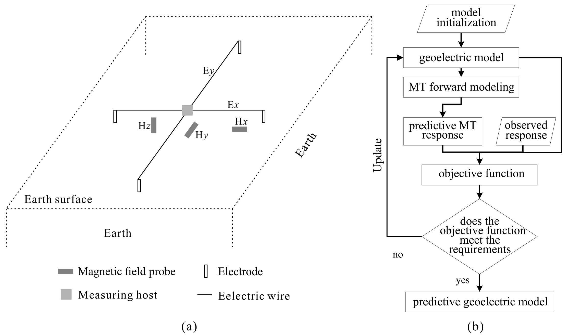
2.1. Forward Modeling

The MT method involves measuring orthogonal components of the electric field E and the magnetic field H at the Earth’s surface (Figure 1a). The electromagnetic field we observe is excited by the natural magnetic field. The frequency is lower than ${10}^5$ Hz so we could ignore the displacement current in the quasi-static approximation of electromagnetic field. When a magnetic field H is applied to the ground, it produces an electric field E through electromagnetic induction. The impedance Z is used to express the relation between the electromagnetic fields as follows [2]:

$$\left[\begin{array}{c}{\mathbf{E}}_x\\ {\mathbf{E}}_y\end{array}\right]=\left[\begin{array}{cc}{\mathbf{Z}}_{xx}& {\mathbf{Z}}_{xy}\\ {\mathbf{Z}}_{yx}& {\mathbf{Z}}_{yy}\end{array}\right]\left[\begin{array}{c}{\mathbf{H}}_x\\ {\mathbf{H}}_y\end{array}\right]$$

(1)

For the one-dimensional case, ${\mathbf{Z}}_{xx}=0$, ${\mathbf{Z}}_{yy}=0$ and ${\mathbf{Z}}_{xy}=-{\mathbf{Z}}_{yx}$. The impedance tensor can be decomposed into two components, corresponding to the apparent resistivity and the phase. For an N-stratum geoelectric model, the apparent resistivity ${\rho }_{\omega }$ and the phase $\phi$ can be derived from the impedance Z regardless of the orientations of the x and y axes as follows:

$$\begin{array}{c}\begin{array}{cc}{\rho }_{\omega }=\frac{{\left|Z_1\right|}^2}{\omega \mu }& \phi ={tan}^{-1}\frac{\mathrm{Im}\left(Z_1\right)}{\mathrm{Re}\left(Z_1\right)}\end{array}\\ \begin{array}{cc}{Z}_m=Z_{om}\frac{1-L_{m+1}{e}^{-2k_m{h}_m}}{1+L_{m+1}{e}^{-2k_m{h}_m}}& L_{m+1}=\frac{Z_{om}+Z_{m+1}}{Z_{om}+Z_{m+1}}\end{array}\\ \begin{array}{ccc}{Z}_N=Z_{oN}& Z_{om}=-i\omega \mu /\phantom{i\omega \mu k_m}{k}_m& k_m=\sqrt{-i\mu {\sigma }_m\omega }\end{array}\end{array}$$

(2)

where $Z_m$ is the impedance at the top of the mth stratum, $Z_{om}$ is the intrinsic impedance of the mth stratum, the magnetic permeability $\mu$ is assigned its free space value and $\omega$ is the angular frequency. For the mth stratum, ${\rho }_m$ is the resistivity and $h_m$ is the thickness. Usually, the apparent resistivity is the observed response that is used to obtain the geoelectric model through inversion.

2.2. Inversions

The MT inversion problem is an optimization problem in which the objective is to predict a model that is close to the real geoelectric structure from the observed response (Figure 1b). The optimization process update the geoelectric model iteratively to find the minimum objective function. The objective function of this optimization problem can be divided into two terms, one corresponding to data fitting and one corresponding to the model smoothness [18]. The data fitting term measures the difference between the observed response and the predicted response (Figure 1b). The smoothness term measures the change in the magnitude of the resistivity of each stratum [21]. The objective function can be expressed as follows:

$$min\mathsf{\Phi }\left(\mathbf{m}\right)=min\left(\lambda {∥{\mathbf{C}}_m\mathbf{m}∥}^2+{∥{\mathbf{C}}_d\left(\mathbf{F}\left[\mathbf{m}\right]-\mathbf{d}\right)∥}^2\right)$$

(3)

where $\mathsf{\Phi }\left(\mathbf{m}\right)$ is the objective function; F is the forward modeling operator; $\mathbf{d}$ represents the observed data; ${\mathbf{C}}_m$ and ${\mathbf{C}}_d$ are the covariance matrices of the model vector and the observed data vector, respectively; and $\lambda$ is the Lagrange multiplier weighting the model smoothness term relative to the total norm. The objective function is updated with the predicted model $\mathbf{m}$, and its value gradually decreases in each iteration.

To minimize the objective function, several iterative methods of linear inversions have been proposed [22,23]. The occam’s inversion is a popular and stable inversion algorithm based on an iterative method in which the model is directly updated in each iteration, causing the value of the objective function to decrease steadily [24,25,26]. The model is updated as follows:

$$\begin{array}{c}{\mathbf{m}}_{k+1}={\left[\frac{1}{\lambda }{\mathbf{C}}_m^T{\mathbf{C}}_m+{\left({\mathbf{C}}_d{\mathbf{J}}_k\right)}^T{\mathbf{C}}_d{\mathbf{J}}_k\right]}^{-1}{\left({\mathbf{C}}_d{\mathbf{J}}_k\right)}^T{\mathbf{C}}_d{\mathbf{d}}_g\\ {\mathbf{d}}_g=\mathbf{d}-\mathbf{F}\left[{\mathbf{m}}_k\right]+{\mathbf{J}}_k{\mathbf{m}}_k\end{array}$$

(4)

The iteration process begins with an initial model guess ${\mathbf{m}}_0$, and the model is updated to ${\mathbf{m}}_k$ in the kth iteration. The optimal model is considered to be found when a maximum number of iterations, a convergence threshold for the objective function or some other termination criterion is reached. In addition, it is important to note that the model parameters are typically expressed in terms of the logarithm of the resistivity in order to reduce the variations in the gradient.

The linear inversion methods can easily become trapped in local minima and require considerable computational effort to calculate the gradient of the objective function [24]. Moreover, they are critically dependent on the initial model [27]. However, global optimization methods based on heuristic algorithms overcome these shortcomings [8,28].

2.3. PSO Optimization

The PSO algorithm will make the population evolve more intelligently after each iteration and can accumulate search knowledge, which is called an evolutionary algorithm [29,30,31]. The PSO algorithm does not use the survival of the fittest but uses a mechanism in which each individual in the population competes with the others to generate the global optimal solution. It generates the optimal solution through information sharing and a mechanism of cooperation between the individuals in the population [32,33].

Suppose the PSO consists of multiple particles. In the D-dimensional search space, the particle swarm contains n particles. The position of the nth particle in the D-dimensional space is defined as $x_i$:

$$\begin{array}{cc}{x}_i=\left(x_{i1},x_{i2},\cdots ,x_{iD}\right),& i=1,2,\cdots ,n.\end{array}$$

(5)

Suppose the current velocity of particle $x_i$ and its individual optimal historical position are $v_i$ and $p_i$, respectively, as follows:

$$\begin{array}{c}{v}_i=\left(v_{i1},v_{i2},\cdots ,v_{iD}\right)\\ p_i=\left(p_{i1},p_{i2},\cdots ,p_{iD}\right).\end{array}$$

(6)

Then, for the entire particle swarm, the global optimal position is $P_g$:

$$p_g=\left(p_{g1},p_{g2},\cdots ,p_{gD}\right).$$

(7)

At the tth moment, the velocity update formula of the dth dimension of particle $x_i$ is:

$$v_{id}\left(t+1\right)=\omega v_{id}\left(t\right)+c_1{r}_1\left(p_{id}\left(t\right)-x_{id}\left(t\right)\right)+c_2{r}_2(p_{gi}\left(t\right)-x_{id}\left(t\right)),$$

(8)

where $\omega$ is the inertia weight and is in the range [0, 1]. ${\mathit{c}}_1$ and ${\mathit{c}}_2$ are the acceleration coefficients. ${\mathit{r}}_1$ and ${\mathit{r}}_2$ are random coefficients, both of which are in [0, 1], which determine the motion of semirandom particles affected by the single and global optimal solutions.

The particle velocity update process has three main parts: the current initial velocity, the self-motion trajectory and self-trajectory correction. The influence of the current speed on the particle update speed can be adjusted by the inertia weight. The influence of the particle’s own trajectory on the particle update speed can be adjusted by the acceleration coefficients and the random coefficients. When the trajectory is inaccurate, it needs to be corrected with the help of global optimization.

For particle $x_i$, we can update the position $x_{id}$ of the dth dimension according to the velocity:

$$x_{id}(t+1)=x_{id}\left(t\right)+v_{id}(t+1).$$

(9)

3. Memetic Strategies

If the particle swarm is regarded as a social population, the three parts of the particle update speed reflect the balance of the population with respect to the global optimum and the local optimum. The particle update speed can be regarded as the cognition of the social population in the evolutionary direction. The evolutionary update speed at the current moment t can provide a reference basis for the evolutionary update speed at the next moment t + 1. During evolution, the evolution of a single particle needs to refer to its own previous evolutionary state and the evolutionary state of the population. The main advantage of the PSO algorithm is that it is simple, effective and easy to implement. However, the PSO algorithm faces premature convergence and easily falls into a local optimal solution [34].

Compared with other group-based methods, the ability of PSO to micromediate and avoid local optima is weaker, which is mainly due to the lack of diversity in the search process [35]. Therefore, we improve the evolutionary diversity of the population in the search process; the basic flow of the cultural strategy is shown in Figure 2.

3.1. Framework

In the memetic strategy, the overall optimization search uses PSO. To optimize an objective function, the first task is to generate the initial population. The initial population in PSO is randomly generated, which may affect the convergence speed of the algorithm and the accuracy of the final solution. In the absence of prior knowledge, we use a method based on opposition learning to replace the random initial population positions as a new initial population strategy. This can increase the chance of reaching the global optimal solution [36].

In the entire iterative search process, we hope that the search range in the early stage is as large as possible to enhance the global optimization capability. We hope that the search range in the search period does not change greatly in order to enhance the local optimization capability. These factors mean that we need to change the inertia weight to adjust the first part of the right-hand term of Equation (8). The dynamic inertia weight is applied to the previous population cognition to provide a reference for the optimization process in the current iteration.

In population evolution, the second part of the right term in Equation (8) represents the synchronization between the current position of the particle and the optimal position of the individual in the iteration. This is the process of the particle revising its own evolutionary path, reflecting the effect of the particle’s own evolutionary experience on its own next evolution. The third part of the right-hand term of Equation (8) shows the process of synchronizing the current position of the particle with the best position of the group. This is the corrective behavior of the particle after observing the evolution of the surrounding particles. This kind of social behavior reflects the group’s information sharing and cooperation.

After obtaining the best population in the current iteration, to further enhance the diversity of the population, we set the mutation of the individual particles for the population. The aim of this operation is to make the optimization process converge stably while maintaining a certain ability to jump out of a local optimum.

3.2. Population Initialization

When there is no prior information, the initial population is usually randomly generated, which often leads to revisiting a hopeless area in the search space [37]. Opposition-based learning (OBL) considers candidate solutions as well as their opposite solutions [38]. OBL introduces a random solution and its corresponding inverse solution, which can yield more than two independent solutions. This randomly generates more promising solutions. OBL has been successfully applied in various population-based evolutionary algorithms [39,40]. To effectively increase the diversity of the initial population, we use the OBL strategy to generate the initial population, which includes two types of populations: a random initial population and an anti-population. The random initial population {$x_{id},d=1,2,\cdots ,D$} is generated randomly according to the form shown in Equation (5). Supposing the inverse population is {$x_{id}^{\prime },d=1,2,\cdots ,D$}, $x_{id}^{\prime }$ can be expressed as:

$$x_{id}^{\prime }=x_{max,d}+x_{min,d}-x_{id},$$

(10)

where $x_{max,d}$ and $x_{min,d}$ are the maximum and minimum values of the dth dimension of particle $x_i$ in the D-dimensional search space. After merging the random initial population and the antipopulation, we select the particles with less fitness to form a new initial population.

3.3. Dynamic Inertia Weight

The inertia weight $\omega$ can limit the search range of particles, which allows the particles to maintain inertia of motion and search in a new area. This means that this new evolution includes old evolutionary habits and experiences. When the inertial weight is relatively high, the new evolution can eliminate the influence of the previous evolutionary experience. This is conducive to expanding the search field, but the convergence speed can easily slow in optimization. When the inertia weight is relatively small, the particle maintains its evolutionary direction based on previous experience. When the evolutionary direction is correct, this will help speed up the convergence rate of the global optimization, but it is easy for the optimization to fall into local extremes [35].

The inertial weight $\omega$ affects the search speed and accuracy. For optimization problems with severe nonlinearity, the use of fixed inertia weights will result in fast convergence, and global optimization is often impossible. For the algorithm to obtain the best results in the optimization process, varying inertia weights need to be used. Using a linearly decreasing inertia weight is a traditional variable inertia weight strategy that can optimize performance well [16]. When the initial inertia weight value is large, the optimal solution range can be found quickly; then, the inertia weight value decreases, and the particles begin to search more finely.

However, because the slope is constant, the speed change always remains at the same level. If the initial iteration does not produce better points, then the accumulation of iterations and the rapid decay of speed may lead to a final local optimal value. Therefore, we use a nonlinear strategy, sine mapping, with ergodicity, nonrepetition and irregularity [34,41] to adjust the inertia weight $\omega$ of PSO. This strategy can not only enhance the population diversity in the search process but also enhance the ability to converge to the global optimum. The dynamic inertia weight based on sine mapping can be expressed as:

$$\begin{array}{ccc}\omega =k_t=\frac{q}{4}sin(\pi k_t-1),& k_t\in (0,1),& t=1,2,3,\cdots ,T,\end{array}$$

(11)

where the range of q is from 0 to 4.

3.4. Accelerating Evolution

The acceleration coefficients ${\mathit{c}}_1$ and ${\mathit{c}}_2$ (Equation (8)) are the cognitive attraction coefficients in the optimization process, and the optimization of the group is controlled by the learning situation. In the early stage of the optimization process, the particles need strong self-cognition and weak social cognition. The global search function is more important. At this time, the particle can traverse as many local extremes as possible in the search space.

In the later stage of optimization, the particles must have strong social cognition and weak self-awareness to avoid falling into local extremes in optimization. The values of the cognitive attraction coefficients reflect the degree of influence of the information exchange on particles, and the information exchange includes the experiential information of the particle itself and the global optimal information. Setting the learning factor to a value that is too large or too small is not conducive to the optimization of the particles, so it is necessary to balance the evolution speed of the particles in the early and late stages of the optimization process.

The enhancing effect of sine-cosine mapping on population diversity and convergence in the optimization process can be used to improve this linear asynchronous strategy. We use sine-cosine acceleration coefficients (SCACs) to adjust the balance between individual cognition and social cognition [42]. The cognitive attraction coefficient can be expressed as:

$$\begin{array}{c}c1=\alpha \times sin((1-\frac{t}{T})\times \frac{\pi }{2})+\delta \hfill \\ c2=\alpha \times \cos ((1-\frac{t}{T})\times \frac{\pi }{2})+\delta ,\hfill \end{array}$$

(12)

where the constants $\alpha$ and $\delta$ are 2 and 0.5, respectively.

3.5. Population Mutation

To enhance the ability to jump out of local extremes, we introduce the mutation operator from the genetic algorithm into the PSO [43]. This can expand the search space of the particles themselves, enhance the diversity of the population and further increase the possibility of finding the optimal solution. The particles will reset with a certain probability after each evolution. When the mutation condition is met, the mutation jumps out of the current position; otherwise, the original position remains unchanged. The particle variation can be expressed as:

$$x_{id}\left(t\right)=r\times ({\mathbf{U}}_x-L_x)/n+({\mathbf{U}}_x-L_x)/2,$$

(13)

where r is uniformly distributed in the range [$-1$, 1], ${\mathbf{U}}_x$ and $L_x$ are the upper and lower limits of a given position and n is 4. The mutation condition is random mutation, and the mutation probability is 10%.

3.6. Fitness

The fitness in the optimization process refers to the objective function setting in MT inversions. The L2 norm is used to define the misfit between the observed MT response data and the predicted response data. The fitness can be expressed as:

$$\begin{array}{c}fit=c_{rho}fi{t}_{rho}+c_{phi}fi{t}_{phi}\\ =c_{rho}{∥1-{\rho }_{pred}/\phantom{{\rho }_{pred}{\rho }_{obs}}{\rho }_{obs}∥}^2+c_{phi}{∥1-{\phi }_{pred}/\phantom{{\phi }_{pred}{\phi }_{obs}}{\phi }_{obs}∥}^2\end{array}$$

(14)

where the overall fitness is composed of apparent resistivity fitness and phase fitness model fitness. Their weight coefficients are $c_{rho}$ and $c_{phi}$. Since the apparent resistivity and phase are variables with different units, in order to transform the apparent resistivity and phase fitness into a unified dimension, we normalize the response data and prediction data.

4. Test Model

We designed two common geoelectric models, a three-layer model and a five-layer model. These models were used to generate synthetic MT response data. Different PSO methods predicted the geoelectric models based on these response data, and the MT responses were obtained through MT forward modeling. Comparing the geoelectric model and the responses predicted by different methods allowed us to test the effect of our memetic strategy.

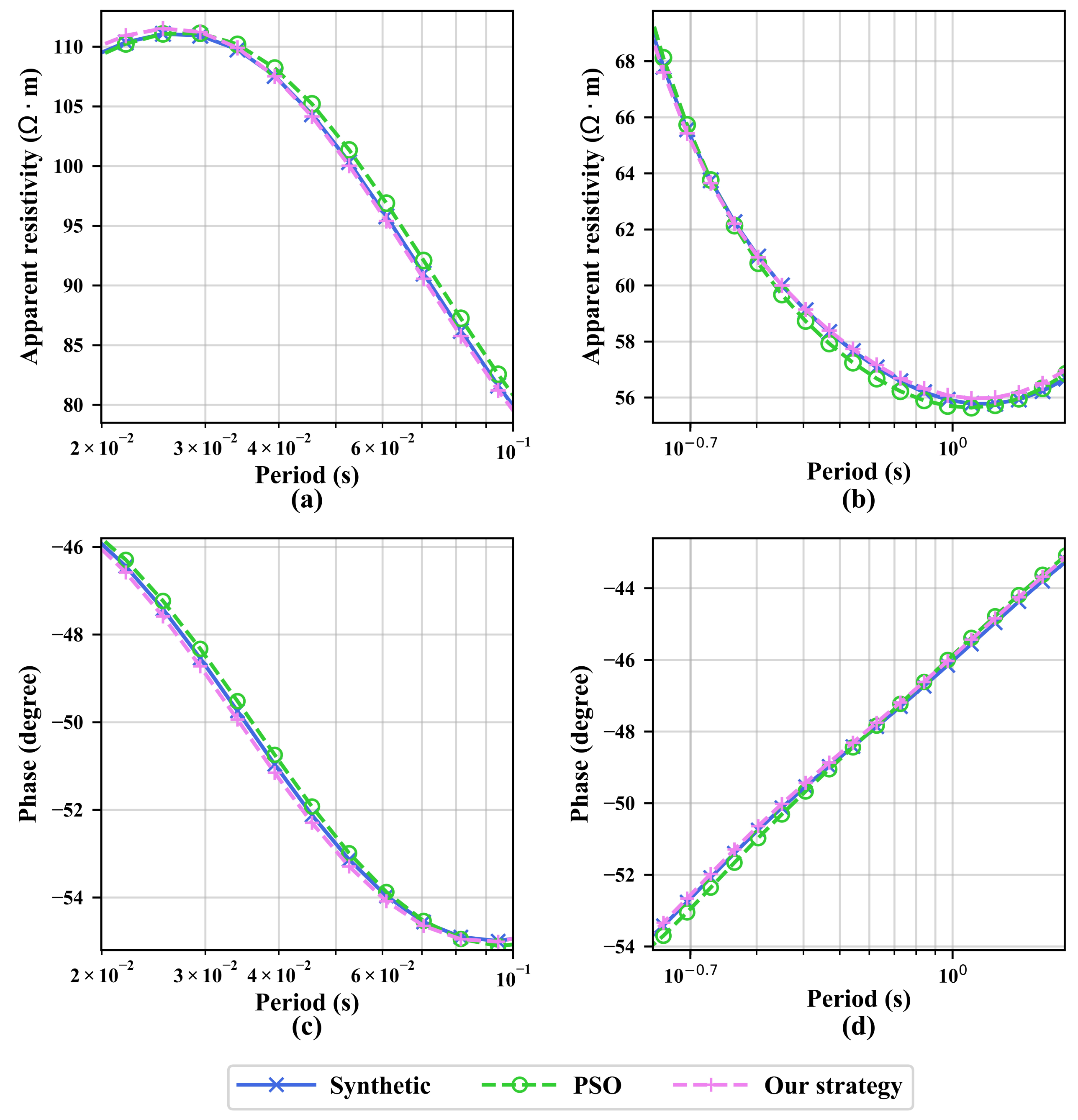
4.1. Three-Layer Model

The three-layer geoelectric model and its MT response are shown in Figure 3. The resistivity values of the geoelectric model are 100 $\mathsf{\Omega }$·m, 20 $\mathsf{\Omega }$·m and 100 $\mathsf{\Omega }$·m. The thicknesses of the geoelectric model are 100 m, 200 m and infinity. We used this model to generate an MT response including the apparent resistivity and phase, which was the supposed response. The geoelectric model predicted by the optimization method based on the supposed MT response contains five values, namely, the resistivity values of the three layers in the geoelectric model and the thickness values of the first two layers. The predicted geoelectric model can be used to regenerate the apparent resistivity and phase response through MT forward modeling.

In the optimization process, the population size is 100. For the supposed three-layer geoelectric model, both traditional PSO and our strategy can obtain good results, but our strategy predicts the results more accurately. From the comparison of the geoelectric models (Figure 3a), the resistivity value of the second layer of the geoelectric model predicted by traditional PSO is less than the supposed value, and the depth value at the bottom of this layer is slightly larger. The resistivity values of the first layer and the third layer predicted by traditional PSO are smaller than the supposed value, and the misfit of the two strata is not as large as the misfit of the second stratum.

From the comparison of the MT responses (Figure 3b,c), the misfit between the MT responses predicted by traditional PSO and the supposed responses is larger. The large misfit is mainly concentrated in the low- and high-frequency ranges. This misfit is more obvious on the apparent resistivity curve. The responses predicted by our strategy, the apparent resistivity curve and the phase curve, perfectly match the supposed response curve.

A detailed comparison of the low-frequency and high-frequency parts is shown in Figure 4. For the apparent resistivity curve, the responses predicted by traditional PSO show a large misfit starting at ${10}^4$ Hz. In the ${10}^4$ Hz–${10}^{2.5}$ Hz interval, this deviation is very obvious (Figure 4a). In the range of ${10}^0$ Hz–${10}^{-1}$ Hz, the misfit of the response predicted by traditional PSO decreases, and it gradually increases as the frequency decreases (Figure 4b). For the same low-frequency and high-frequency ranges, the characteristics of the misfit of apparent resistivity are different. In the low-frequency range, the misfit of traditional PSO always exists and is not concentrated in the ${10}^4$ Hz–${10}^{2.5}$ Hz range, similar to the misfit of the apparent resistivity curve (Figure 4c). The deviation of the response predicted by traditional PSO has the same characteristics in the high-frequency range (Figure 4d).

For the traditional PSO method, our memetic strategy has four improved steps, namely, group initialization with OBL, using DIWs to integrate empirical cognition, using the cognitive attraction coefficient to accelerate population evolution and PM. We call them PSO-OBL, PSO-OBL-DIW, PSO-OBL-DIW-SCAC and PSO-OBL-DIW-SCAC-PM. Combining traditional PSO and these four improvements, the corresponding optimization process is shown in Figure 5.

Using OBL can determine the appropriate initial population more accurately, which can enable the search process to find the appropriate global optimal search direction in the early stage and accelerate convergence. At the early stage, the fitness decline rate of PSO-OBL is faster than that of traditional PSO. Adding DIWs based on sine mapping can enable the evolution of the population to better combine with previous cognitive experience. Therefore, after 17 iterations, the fitness decline rate of PSO-OBL-DIW is faster than that of PSO-OBL.

On the basis of PSO-OBL-DIW, the advantages of SCACs in effectively integrating individual experience and group experience are used to reflect the faster fitness decline rate of PSO-OBL-DIW-SCAC. The final fitness also remained at a low level. After the population evolution, the population was allowed to continue to produce genetic mutations, which can further accelerate the convergence of the optimization process. The final fitness of PSO-OBL-DIW-SCAC-PM was generally lower than that of PSO-OBL-DIW-SCAC.

The accuracy comparison of the three-layer geoelectric models predicted by different methods is shown in

Table 1. Accuracy comparison of three-layer geoelectric model predicted by different methods.

		$\mathit{\rho }$($\mathsf{\Omega }$·m)			h(m)		Fitness
		${\rho }_{\mathbf{1}}$	${\rho }_{\mathbf{2}}$	${\rho }_{\mathbf{3}}$	${\mathit{h}}_{\mathbf{1}}\left(\mathbf{m}\right)$	${\mathit{h}}_{\mathbf{2}}\left(\mathbf{m}\right)$
Supposed model		100.00	20.00	100.00	100.00	200.00
PSO	model	98.61	19.38	98.27	102.58	189.95	$3.32\times {10}^{-3}$
	misfit ${}^1$	1.39	3.08	1.73	2.58	5.02
SO-OBL	model	99.84	20.42	100.12	97.36	205.08	$1.95\times {10}^{-3}$
	misfit	0.16	2.09	0.12	2.64	2.54
PSO-OBL-DIW	model	100.16	20.37	100.21	98.21	205.27	$5.94\times {10}^{-4}$
	misfit	0.16	1.87	0.21	1.78	2.64
PSO-OBL-DIW-SCAC	model	100.05	20.12	100.06	99.41	201.61	$4.03\times {10}^{-4}$
	misfit	0.05	0.58	0.06	0.59	0.81
PSO-OBL-DIW-SCAC-PM	model	99.96	19.97	100.03	200.15	99.86	$2.39\times {10}^{-4}$
	misfit	0.04	0.17	0.03	0.08	0.14

${}^1$ The misfit = $|v_{pred}-v_{supp}|/v_{supp}$, $v_{pred}$ is the predictive value, $v_{supp}$ is the parameter of the supposed model.

. The misfit between the predicted value and the supporting value can be expressed as the absolute value of the normalized error. The misfit trends of different methods are consistent with the final fitness trend of optimization. Each improvement increases the prediction accuracy of the resistivity value and the thickness value in the geoelectric model.

4.2. Five-Layer Model

Our method is suitable not only for three-layer models but also for more complex five-layer models. The five-layer geoelectric model and its MT responses are shown in Figure 6. The resistivity values of the geoelectric model are 100 $\mathsf{\Omega }$·m, 20 $\mathsf{\Omega }$·m, 200 $\mathsf{\Omega }$·m, 50 $\mathsf{\Omega }$·m and 100 $\mathsf{\Omega }$·m. The thicknesses of the geoelectric model are 1000 m, 500 m, 1000 m, 2000 m and infinity. The geoelectric model predicted by the optimization method based on the supposed MT responses contains nine values, namely, the resistivity values of the five layers in the geoelectric model and the thickness values of the first four layers.

For the supposed five-layer geoelectric model, both traditional PSO and our strategy can achieve good results, but our strategy predicts the results more accurately. From the comparison of geoelectric models (Figure 6a), the resistivity value of the third layer of the geoelectric model predicted by traditional PSO is greater than the supposed value, and the top depth and the bottom depth are both larger. The bottom depth of the fourth layer of the geoelectric model predicted by traditional PSO is obviously smaller than the supposed value, and the misfit reaches approximately 200 m.

From the comparison of the MT responses (Figure 6b,c), the responses predicted by traditional PSO have a greater misfit with the supposed responses, and this deviation is mainly concentrated in the mid-frequency range. Similar to the results of the three-layer model (Figure 4b,c), the responses predicted by our strategy, the apparent resistivity curve and the phase curve, perfectly match the assumed response curve.

A detailed comparison of the middle frequency range is shown in Figure 7. The middle frequency interval can be divided into two subintervals for evaluation: the 50 Hz–1 Hz interval (Figure 7a,c) and the ${10}^{0.8}$ Hz–${10}^{-0.3}$ Hz interval (Figure 7b,d). In the first interval, the apparent resistivity and phase misfit of traditional PSO are not concentrated in a certain frequency range but have wide coverage. In the second interval, the apparent resistivity misfit of traditional PSO is mainly concentrated in the middle frequency range, and the phase misfit is mainly concentrated in the higher frequency range.

For the supposed MT responses of the five-layer geoelectric model, we use traditional PSO, PSO-OBL, PSO-OBL-DIW, PSO-OBL-DIW-SCAC and PSO-OBL-DIW-SCAC-PM to optimize the misfit of the supposed responses and predicted responses. The corresponding optimization process is shown in Figure 8.

OBL allows the optimization process to find the appropriate global optimal search direction at an early stage and speed up the convergence. This shows the effectiveness of using OBL to determine a suitable initial population. The advantages of PSO-OBL-DIW began to manifest after the 10th evolutionary iteration, indicating that the combination of PSO-OBL-DIW with previous evolutionary cognitive experience is conducive to obtaining a more accurate evolutionary direction for the population. The effective integration of individual experience and group experience through SCACs is still obvious in promoting the optimization process. PSO-OBL-DIW-SCAC changed after the fifth evolutionary iteration to accelerate the convergence speed of fitness and keep the convergence trend stable. Although we set only a 10% gene mutation probability, PSO-OBL-DIW-SCAC-PM still has a great advantage in fitness convergence over PSO-OBL-DIW-SCAC.

Table 2. Accuracy comparison of five-layer geoelectric model predicted by different methods.

		$\mathit{\rho }$($\mathsf{\Omega }$·m)					h(m)				Fitness
		${\rho }_{\mathbf{1}}$	${\rho }_{\mathbf{2}}$	${\rho }_{\mathbf{3}}$	${\rho }_{\mathbf{4}}$	${\rho }_{\mathbf{5}}$	${\mathit{h}}_{\mathbf{1}}\left(\mathbf{m}\right)$	${\mathit{h}}_{\mathbf{2}}\left(\mathbf{m}\right)$	${\mathit{h}}_{\mathbf{3}}\left(\mathbf{m}\right)$	${\mathit{h}}_{\mathbf{4}}\left(\mathbf{m}\right)$
Supposed model		100.00	20.00	200.00	50.00	100.00	1000.00	500.00	1000.00	2000.00
PSO	model	100.11	20.34	207.38	49.67	98.51	1009.82	530	1019.5	1806.08	$8.60\times {10}^{-3}$
	misfit ${}^1$	0.11	1.68	3.69	0.67	1.49	0.98	6	1.95	9.7
PSO-OBL	model	99.79	20.21	200.52	48.3	100.81	973.19	483.79	968.88	1984.67	$5.10\times {10}^{-3}$
	misfit	0.21	1.04	0.26	3.39	0.81	2.68	3.24	3.11	0.77
PSO-OBL-DIW	model	99.53	19.96	195	50.4	98.03	1012.72	510.31	1008.9	1977.88	$1.72\times {10}^{-4}$
	misfit	0.47	0.22	2.5	0.79	1.97	1.27	2.06	0.89	1.11
PSO-OBL-DIW-SCAC	model	100	20.31	198.23	50.32	100.04	996.66	508.88	990.29	2021.54	$9.18\times {10}^{-5}$
	misfit	0	1.53	0.88	0.64	0.04	0.33	1.78	0.97	1.08
PSO-OBL-DIW-SCAC-PM	model	100.36	20.06	200.48	50.34	100.8	990.26	496.39	996.2	1988.36	$2.52\times {10}^{-6}$
	misfit	0.36	0.3	0.24	0.69	0.8	0.97	0.72	0.38	0.58

${}^1$ The misfit = $|v_{pred}-v_{supp}|/v_{supp}$, $v_{pred}$ is the predictive value, $v_{supp}$ is the parameter of the supposed model.

shows an accuracy comparison of different methods used to predict the five-layer geoelectric model. The misfit between the predicted value and the supposed value can be expressed as the absolute value of the normalized error. The number of parameters of the five-layer geoelectric model is greater than that of the three-layer geoelectric model, and the accuracy of the resistivity and thickness values predicted in the five-layer geoelectric model test is not as good as that in the three-layer geoelectric model test. However, the effect of each improvement on the prediction accuracy is consistent with the effect in the three-layer geoelectric model test. This shows that the effect of our memetic strategy can be applied to a more complex five-layer geoelectric model.

5. Stability Evaluation

To evaluate the stability of our strategy for MT inversions, we conducted a noise immunity test and a test with actual data. In the tests, we compared our improvement strategy with traditional PSO.

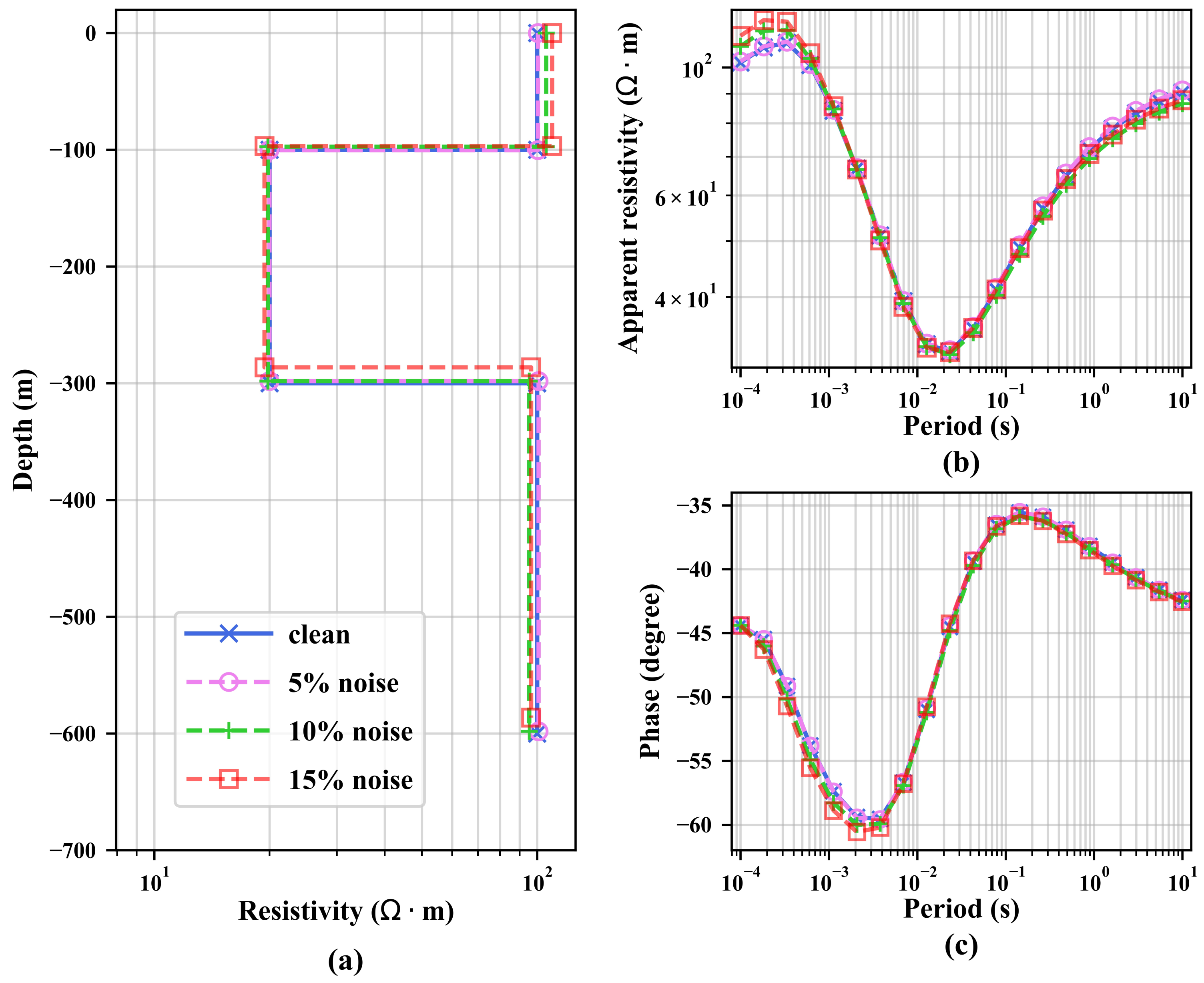
5.1. Noise Immunity Test

In the noise immunity test, we designed three different levels of random noise and added noise to the supposed MT responses of the three-layer geoelectric model and the five-layer geoelectric model. The noise levels are 5%, 10% and 15%, respectively. The MT responses of the three-layer geoelectric model with noise are shown in Figure 9.

For the responses of the three-layer geoelectric model, 5% of the noise has basically no effect on our final prediction results. The predicted geoelectric model and responses perfectly match the assumed geoelectric model and responses. From the comparison of the geoelectric models (Figure 10a), 10% noise and 15% noise cause the predicted resistivity value of the first layer of the geoelectric model to deviate, and the greater the noise is, the greater the deviation. However, the thickness of the first layer is basically consistent with the supposed value. The predicted resistivity value of the second layer is also not affected by noise, but 15% noise makes the predicted thickness smaller than the supposed value. The predicted resistivity value in the third layer corresponding to 10% noise and 15% noise is smaller than the supposed value.

Table 3. Comparison of the accuracy of the predicted three-layer geoelectric model under different noise levels.

		$\mathit{\rho }$($\mathsf{\Omega }$·m)			h(m)		Fitness
		${\rho }_{\mathbf{1}}$	${\rho }_{\mathbf{2}}$	${\rho }_{\mathbf{3}}$	${\mathit{h}}_{\mathbf{1}}\left(\mathbf{m}\right)$	${\mathit{h}}_{\mathbf{2}}\left(\mathbf{m}\right)$
Supposed model		100.00	20.00	100.00	200.00	100.00
5% noise	model	100.42	19.98	100.8	100.25	197.8	$2.19\times {10}^{-2}$
	misfit ${}^1$	0.42	0.09	0.8	0.24	1.1
10% noise	model	105.6	19.8	95.34	97.31	200.7	$4.25\times {10}^{-2}$
	misfit	5.6	0.98	4.66	2.69	0.36
15% noise	model	109.44	19.4	96.43	96.72	189.6	$6.63\times {10}^{-2}$
	misfit	9.44	2.99	3.57	3.28	5.2

${}^1$ The misfit = $|v_{pred}-v_{supp}|/v_{supp}$, $v_{pred}$ is the predictive value, $v_{supp}$ is the parameter of the supposed model.

shows the accuracy comparison of the detailed predictive electrical model.

From the comparison of the MT responses (Figure 10b,c), the predicted value misfit caused by 10% noise and 15% noise is in the same frequency range. For the apparent resistivity curves, the misfit is concentrated in the low- and high-frequency regions, and the misfit in the low-frequency region is larger than that in other regions (Figure 10b). For the phase curves, the misfit is concentrated in the low-frequency to mid-frequency region, and the misfit in the high-frequency data is milder (Figure 10c).

For the MT response of the synthetic five-layer geoelectric model, the response after adding noise is shown in Figure 11. For the noise-containing responses of the five-layer geoelectric model, the influence of noise is obviously greater than that in the three-layer model. From the comparison of the geoelectric models (Figure 12a), the predicted resistivity values are close to the supposed values in the first three layers. For the second stratum, the predicted value for 5% noise has a slight deviation. 10% noise and 15% noise increase the deviation. The maximum misfit of the predicted resistivity of 15% noise is close to 15%, and the maximum misfit of the predicted layer thickness is close to 10%.

Table 4. Comparison of the accuracy of the predicted five-layer geoelectric model under different noise levels.

		$\mathit{\rho }$($\mathsf{\Omega }$·m)					h(m)				Fitness
		${\rho }_{\mathbf{1}}$	${\rho }_{\mathbf{2}}$	${\rho }_{\mathbf{3}}$	${\rho }_{\mathbf{4}}$	${\rho }_{\mathbf{5}}$	${\mathit{h}}_{\mathbf{1}}\left(\mathbf{m}\right)$	${\mathit{h}}_{\mathbf{2}}\left(\mathbf{m}\right)$	${\mathit{h}}_{\mathbf{3}}\left(\mathbf{m}\right)$	${\mathit{h}}_{\mathbf{4}}\left(\mathbf{m}\right)$
Supposed mode		100.00	20.00	200.00	50.00	100.00	1000.00	500.00	1000.00	2000.00
5% noise	model	99.47	19.98	203.61	48.63	102.5	1016.27	505.19	1017	2020.14	0.0241
	misfit ${}^1$	0.53	0.12	1.81	2.73	2.5	1.63	1.038	1.7	1.01
10% noise	model	99.54	20.09	199.34	54.21	94.39	1025.08	502.03	989.19	2091.82	0.0491
	misfit	0.46	0.44	0.33	8.41	5.61	2.51	0.41	1.08	4.59
15% noise	model	97.28	19.77	209.19	57.04	105.71	1050.71	549.93	1054.34	2058.1	0.077
	misfit	2.71	1.13	4.6	14.08	5.71	5.07	9.99	5.43	2.91

${}^1$ The misfit = $|v_{pred}-v_{supp}|/v_{supp}$, $v_{pred}$ is the predictive value, $v_{supp}$ is the parameter of the supposed model.

shows the accuracy comparison of the detailed predictive geoelectric model.

From the comparison of the MT responses (Figure 12b,c), the predicted response for 5% noise has a small deviation from the supposed value, and the two types of responses are basically consistent. A 10% noise level will increase the deviation, and 15% noise will cause the most serious deviation. In particular, with the deviation of the apparent resistivity response, 15% noise causes the deviation to cover almost the whole frequency band. For the phase responses, the deviation caused by 15% noise covers most of the frequency range, from low to intermediate frequencies.

5.2. Real Application Data

The COPROD2 dataset is a public dataset for testing the MT inversion effect, which contains measured MT response data [44]. However, the underground structure is not accurately proven. We can evaluate the inversion effect by observing the difference in fit between the predicted responses and the measured responses. The prediction effect of the proposed memetic strategy is compared with that of the traditional PSO method. The COPROD2 data contain 35 observation points. We selected the fifth, tenth, 15th and 20th observation points as our test data. The measured data can be divided into YX mode and XY mode according to the polarization mode. The prediction results under the two modes are shown in Figure 13 and Figure 14.

Among the results for the four observation stations, our memetic strategy prediction results are significantly better than the traditional PSO prediction results. When the measured responses fluctuate gently, the predicted responses can fit the measured responses. However, the prediction results of traditional PSO are consistent only with the measured responses in the change trend, and the predicted value has a large deviation. When the measured responses fluctuate violently, the predicted results of the two methods are quite different from the measured response.

Considering the volume effect of electromagnetic waves and the static effect near the surface, the response curve of the one-dimensional geoelectric model has difficulty matching the measured curve perfectly. In addition, the violent fluctuations in the measured data are mainly concentrated in the high-frequency range, which is also influenced by human noise, magnetic storms and substation interference. This nonrandom noise increases the difficulty of inversions.

6. Conclusions

For MT inversions, we propose a memetic strategy on the basis of traditional PSO, which includes four parts: opposition-based learning, dynamic inertia weights, sine-cosine acceleration coefficients and gene mutation. The test results of the different models show that reverse learning can selectively enhance the population diversity and accelerate the optimization process. The dynamic inertia weights based on sine mapping can strengthen the optimization ability by fusing previous cognitive experience. By balancing the influence of individual cognition and group cognition on the evolutionary process, the sine-cosine acceleration coefficients can improve the global optimization capability in the early stages of the optimization process and maintain convergence stability in the later stages. Genetic mutation can further strengthen the ability to find the best solution by enhancing the population diversity.

The noise test verifies that this memetic strategy can improve the noise immunity of PSO. Moreover, the proposed strategy outperforms the traditional PSO method on the measured MT data. We have greatly improved the ability of PSO to invert MT data by enhancing the diversity of the population and fusing the individual and social cognition of the population.

References

1. Seillé, H.; Visser, G. Bayesian inversion of magnetotelluric data considering dimensionality discrepancies. Geophys. J. Int. 2020, 223, 1565–1583. [Google Scholar] [CrossRef]
2. Howard, A.Q. Special Issue on Electromagnetic Methods in Applied Geophysics—Introduction. IEEE Trans. Geosci. Remote Sens. 1984, 22, 2. [Google Scholar]
3. Zhdanov, M. Foundations of Geophysical Electromagnetic Theory and Methods; Elsevier: Oxford, UK, 2009. [Google Scholar]
4. Ramananjaona, C.; MacGregor, L.; Andréis, D. Sensitivity and inversion of marine electromagnetic data in a vertically anisotropic stratified earth. Geophys. Prospect. 2011, 59, 341–360. [Google Scholar] [CrossRef]
5. Kordy, M.; Wannamaker, P.; Maris, V.; Cherkaev, E.; Hill, G. 3-D magnetotelluric inversion including topography using deformed hexahedral edge finite elements and direct solvers parallelized on SMP computers—Part I: Forward problem and parameter Jacobians. Geophys. J. Int. 2015, 204, 74–93. [Google Scholar] [CrossRef]
6. Constable, S.C.; Parker, R.L.; Constable, C.G. Occam’s inversion: A practical algorithm for generating smooth model from electromagnetic sounding data. Geophysics 1987, 52, 289–300. [Google Scholar] [CrossRef]
7. Li, R.; Hu, X.; Xu, D.; Liu, Y.; Yu, N. Characterizing the 3D hydrogeological structure of a debris landslide using the transient electromagnetic method. J. Appl. Geophys. 2020, 175, 103991. [Google Scholar] [CrossRef]
8. Conway, D.; Alexander, B.; King, M.; Heinson, G.; Kee, Y. Inverting magnetotelluric responses in a three-dimensional earth using fast forward approximations based on artificial neural networks. Comput. Geosci. 2019, 127, 44–52. [Google Scholar] [CrossRef]
9. Grana, D.; Fjeldstad, T.; Omre, H. Bayesian Gaussian Mixture Linear Inversion for Geophysical Inverse Problems. Math. Geosci. 2017, 49, 493–515. [Google Scholar] [CrossRef]
10. Wang, G.G.; Tan, Y. Improving Metaheuristic Algorithms With Information Feedback Models. IEEE Trans. Cybern. 2019, 49, 542–555. [Google Scholar] [CrossRef]
11. Wang, G.G.; Guo, L.; Gandomi, A.H.; Hao, G.S.; Wang, H. Chaotic Krill Herd algorithm. Inf. Sci. 2014, 274, 17–34. [Google Scholar] [CrossRef]
12. Sharma, S.P.; Biswas, A. Global nonlinear optimization for the estimation of static shift and interpretation of 1-D magnetotelluric sounding data. Ann. Geophys. 2011, 54, 249–264. [Google Scholar]
13. Xiang, E.; Guo, R.; Liu, J.; Ren, Z.; Dong, H. Efficient hierarchical trans-dimensional Bayesian inversion of magnetotelluric data. Geophys. J. Int. 2018, 213, 3. [Google Scholar] [CrossRef]
14. Batista, J.D.C.; Sampaio, E.E.S. Magnetotelluric inversion of one- and two-dimensional synthetic data based on hybrid genetic algorithms. Acta Geophys. 2019, 67, 1365–1377. [Google Scholar] [CrossRef]
15. Pace, F.; Santilano, A.; Godio, A. Particle Swarm Optimization of 2D Magnetotelluric data. Geophysics 2019, 84, 1–59. [Google Scholar] [CrossRef]
16. Shi, Y.; Obaiahnahatti, B. A Modified Particle Swarm Optimizer. In Proceedings of the IEEE Conference on Evolutionary Computation, Anchorage, AK, USA, 4–9 May 1998; Volume 6, pp. 69–73. [Google Scholar]
17. Jordehi, A.R. Time varying acceleration coefficients particle swarm optimisation (TVACPSO): A new optimisation algorithm for estimating parameters of PV cells and modules. Energy Conv. Manag. 2016, 129, 262–274. [Google Scholar] [CrossRef]
18. Ali, A.F.; Tawhid, M.A. A hybrid particle swarm optimization and genetic algorithm with population partitioning for large scale optimization problems. Ain Shams Eng. J. 2017, 8, 191–206. [Google Scholar] [CrossRef] [Green Version]
19. Fernandes, I.F.; Silva, I.R.D.M.; Goldbarg, E.F.G.; Monteiro, S.M.D.; Goldbarg, M.C. A PSO-inspired architecture to hybridise multi-objective metaheuristics. Memet. Comput. 2020, 12, 235–249. [Google Scholar] [CrossRef]
20. Zhang, Z.; Wong, W.K.; Tan, K.C. Competitive swarm optimizer with mutated agents for finding optimal designs for nonlinear regression models with multiple interacting factors. Memet. Comput. 2020, 12, 219–233. [Google Scholar] [CrossRef]
21. Commer, M.; Newman, G.A. New advances in three-dimensional controlled-source electromagnetic inversion. Geophys. J. Int. 2008, 172, 513–535. [Google Scholar] [CrossRef]
22. Yang, D.; Oldenburg, D.W.; Haber, E. 3-D inversion of airborne electromagnetic data parallelized and accelerated by local mesh and adaptive soundings. Geophys. J. Int. 2014, 196, 582. [Google Scholar] [CrossRef] [Green Version]
23. Zhdanov, M.S.; Uma, M.; Wilson, G.A.; Velikhov, E.P.; Black, N.; Gribenko, A.V. Iterative electromagnetic migration for 3D inversion of marine controlled: Ource electromagnetic data. Geophys. Prospect. 2011, 59, 1101–1113. [Google Scholar] [CrossRef]
24. Siripunvaraporn, W. Three-dimensional magnetotelluric inversion: An introductory guide for developers and users. Surv. Geophys. 2012, 33, 5–27. [Google Scholar] [CrossRef]
25. Li, R.; Hu, X.; Li, J. Pseudo-3D constrained inversion of transient electromagnetic data for a polarizable SMS hydrothermal system in the Deep Sea. Stud. Geophys. Geod. 2018, 62, 512–533. [Google Scholar] [CrossRef]
26. Groothedlin, C.D.D.; Constable, S.C. Occam’s inversion to generate smooth, two-dimensional models from magnetotelluric data. Geophysics 1990, 55, 1613–1624. [Google Scholar] [CrossRef]
27. Sasaki, Y. Full 3-D inversion of electromagnetic data on PC. J. Appl. Geophys. 2001, 46, 45–54. [Google Scholar] [CrossRef]
28. Thakur, P.; Srivastava, D.C.; Gupta, P.K. The genetic algorithm: A robust method for stress inversion. J. Struct. Geol. 2017, 94, 227–239. [Google Scholar] [CrossRef]
29. Neri, F.; Cotta, C. Memetic algorithms and memetic computing optimization: A literature review. Swarm Evol. Comput. 2012, 2, 1–14. [Google Scholar] [CrossRef]
30. Wang, D.; Tan, D.; Liu, L. Particle swarm optimization algorithm: An overview. Soft Comput. 2018, 22, 387–408. [Google Scholar] [CrossRef]
31. Liu, B.F.; Chen, H.M.; Chen, J.H.; Hwang, S.F.; Ho, S.Y. MeSwarm: Memetic particle swarm optimization. In Proceedings of the Genetic and Evolutionary Computation Conference, GECCO 2005, Washington, DC, USA, 25–29 June 2005. [Google Scholar]
32. Chiam, S.; Tan, K.; Al-Mamun, A. A memetic model of evolutionary PSO for computational finance applications. Expert Syst. Appl. 2009, 36, 3695–3711. [Google Scholar] [CrossRef]
33. Gou, J.; Lei, Y.X.; Guo, W.P.; Wang, C.; Cai, Y.Q.; Luo, W. A novel improved particle swarm optimization algorithm based on individual difference evolution. Appl. Soft. Comput. 2017, 57, 468–481. [Google Scholar] [CrossRef]
34. Clerc, M.; Kennedy, J. The particle swarm-explosion, stability, and convergence in a multidimensional complex space. IEEE Trans. Evol. Comput. 2002, 6, 58–73. [Google Scholar] [CrossRef] [Green Version]
35. Chauhan, P.; Deep, K.; Pant, M. Novel inertia weight strategies for particle swarm optimization. Memet. Comput. 2013, 5, 229–251. [Google Scholar] [CrossRef]
36. Zhou, Y.; Hao, J.K.; Duval, B. Opposition-based Memetic Search for the Maximum Diversity Problem. IEEE Trans. Evol. Comput. 2017, 21, 731–745. [Google Scholar] [CrossRef] [Green Version]
37. Ma, X.; Zhang, Q.; Tian, G.; Yang, J.; Zhu, Z. On Tchebycheff decomposition approaches for multiobjective evolutionary optimization. IEEE Trans. Evol. Comput. 2017, 22, 226–244. [Google Scholar] [CrossRef]
38. Tizhoosh, H.R. Opposition-based learning: A new scheme for machine intelligence. In Proceeding of the International Conference on Computational Intelligence for Modelling, Control and Automation and International Conference on Intelligent Agents, Web Technologies and Internet Commerce (CIMCA-IAWTIC’06), Vienna, Austria, 28–30 November 2005; Volume 1, pp. 695–701. [Google Scholar]
39. Wang, W.; Wang, H.; Sun, H.; Rahnamayan, S. Using opposition-based learning to enhance differential evolution: A comparative study. In Proceeding of the 2016 IEEE Congress on Evolutionary Computation (CEC), Vancouver, BC, Canada, 24–29 July 2016; pp. 71–77. [Google Scholar]
40. Ma, X.; Liu, F.; Qi, Y.; Gong, M.; Yin, M.; Li, L.; Jiao, L.; Wu, J. MOEA/D with opposition-based learning for multiobjective optimization problem. Neurocomputing 2014, 146, 48–64. [Google Scholar] [CrossRef]
41. Bansal, J.C.; Singh, P.; Saraswat, M.; Verma, A.; Jadon, S.S.; Abraham, A. Inertia weight strategies in particle swarm optimization. In Proceeding of the 2011 Third World Congress on Nature and Biologically Inspired Computing, Salamanca, Spain, 19–21 October 2011; IEEE: New York, NY, USA, 2011; pp. 633–640. [Google Scholar]
42. Chen, K.; Zhou, F.; Yin, L.; Wang, S.; Wang, Y.; Wan, F. A hybrid particle swarm optimizer with sine cosine acceleration coefficients. Inf. Sci. 2018, 422, 218–241. [Google Scholar] [CrossRef]
43. Ibrahim, A.O.; Shamsuddin, S.M.; Abraham, A.; Qasem, S.N. Adaptive memetic method of multi-objective genetic evolutionary algorithm for backpropagation neural network. Neural Comput. Appl. 2019, 31, 4945–4962. [Google Scholar] [CrossRef]
44. Beusekom, A.; Parker, R.; Bank, R.; Gill, P.; Constable, S. The 2-D magnetotelluric inverse problem solved with optimization. Geophys. J. Int. 2011, 184, 639–650. [Google Scholar] [CrossRef] [Green Version]
Figure 1. Basic introduction of the magnetotelluric (MT) method. (a) shows the layout of the MT signal acquisition system. The electrodes connected by wires is used to obtain electric field data, and the magnetic field probes are used for collecting magnetic field data. The host is used to record the signal at various frequencies. (b) The application of the optimization process in MT inversions.
Mathematics 09 00519 g001
Figure 2. Flow chart of memetic strategy for MT inversions.
Mathematics 09 00519 g002
Figure 3. The three-layer geoelectric model and its MT response predicted by traditional PSO and by our strategy. (ac) represent the geoelectric model, apparent resistivity responses and represent phase responses, respectively. The blue lines represent the supposed three-layer geoelectric model and its MT responses. The green lines represent the geoelectric model predicted by the traditional PSO and its MT responses. The purple lines represent the geoelectric model predicted by our strategy and its MT responses.
Mathematics 09 00519 g003
Figure 4. Comparison of the MT response in special frequency bands for the three-layer model. (a,b) represent apparent resistivity curves, and (c,d) represent phase curves. The blue lines represent the supposed MT responses. The green lines represent the MT responses predicted by traditional PSO. The purple lines represent the MT responses predicted by our strategy.
Mathematics 09 00519 g004
Figure 5. Comparison of the optimization process of different strategies in the three-layer geoelectric model test. The number of evolutionary iterations is 50. The blue line represents the optimization process of traditional PSO. The orange line represents the optimization process of PSO-opposition-based learning (OBL). The green line represents the optimization process of PSO-OBL-dynamic inertia weight (DIW). The red line represents the optimization process of PSO-OBL-DIW-sine-cosine acceleration coefficient (SCAC). The violet line represents the optimization process of PSO-OBL-DIW-SCAC-population mutation (PM).
Mathematics 09 00519 g005
Figure 6. The five-layer geoelectric model and its MT response predicted by traditional PSO and our strategy. (ac) represent the geoelectric model, apparent resistivity responses and represent phase responses, respectively. The blue lines represent the supposed three-layer geoelectric model and its MT responses. The green lines represent the geoelectric model predicted by traditional PSO and its MT responses. The purple lines represent the geoelectric model predicted by our strategy and its MT responses.
Mathematics 09 00519 g006
Figure 7. Comparison of the MT response in special frequency bands for the five-layer model. (a,b) represent apparent resistivity curves, and (c,d) represent phase curves. The blue lines represent the supposed MT responses. The green lines represent the MT responses predicted by traditional PSO. The purple lines represent the MT responses predicted by our strategy.
Mathematics 09 00519 g007
Figure 8. Comparison of the optimization process of different strategies in the five-layer geoelectric model test. The number of evolutionary iterations is 50. The blue line represents the supposed MT response. The green line represents the optimization process of traditional PSO. The yellow line represents the optimization process of PSO-OBL. The green line represents the optimization process of PSO-OBL-DIW. The red line represents the optimization process of PSO-OBL-DIW-SCAC. The red line represents the optimization process of PSO-OBL-DIW-SCAC-PM.
Mathematics 09 00519 g008
Figure 9. Supposed MT responses of a three-layer geoelectric model with different levels of noise. (a,b) represent the MT responses when the noise level is 5%. (c,d) represent the MT responses when the noise level is 10%. (e,f) represent the MT responses when the noise level is 15%. (a,c,e) represent the apparent resistivity responses. (b,d,f) represent the apparent resistivity responses. The blue lines represent the clean supposed responses. The red dots indicate the noisy responses. The red lines are the error bars between the noisy data and clean data.
Mathematics 09 00519 g009
Figure 10. The predicted three-layer geoelectric models and their MT responses under noisy conditions. (ac) represent the geoelectric model, apparent resistivity responses and phase responses, respectively. The blue lines represent the supposed three-layer electrical model and clean MT responses, and the purple lines represent the predicted geoelectric model and its MT responses when the noise level is 5%. The green lines represent the predicted geoelectric model and its MT responses when the noise level is 10%. The red lines represent the predicted geoelectric model and its MT responses when the noise level is 15%.
Mathematics 09 00519 g010
Figure 11. Supposed MT responses of a five-layer geoelectric model with different levels of noise. (a,b) represent the MT responses when the noise level is 5%. (c,d) represent the MT responses when the noise level is 10%. (e,f) represent the MT responses when the noise level is 15%. (a,c,e) represent the apparent resistivity responses. (b,d,f) represent the apparent resistivity responses. The blue lines represent the clean supposed responses. The red dots indicate the noisy responses. The red lines are the error bars between the noisy data and clean data.
Mathematics 09 00519 g011
Figure 12. The predicted five-layer geoelectric models and their MT responses under noisy conditions. (ac) represent the geoelectric model, apparent resistivity responses and phase responses, respectively. The blue lines represent the supposed three-layer electrical model and clean MT responses, and the purple lines represent the predicted geoelectric model and its MT responses when the noise level is 5%. The green lines represent the predicted geoelectric model and its MT responses when the noise level is 10%. The red lines represent the predicted geoelectric model and its MT responses when the noise level is 15%.
Mathematics 09 00519 g012
Figure 13. Comparison of the predicted and measured responses in YX mode. (ad) represent the apparent resistivity response curves, and (eh) represent the phase response curves. (a,e) represent the response curves of the fifth observation station, (b,f) represent the response curves of the tenth observation station, (c,g) represent the response curves of the 15th observation station, and (d,h) represent the response curves of the 20th observation station. The blue lines represent the measured response curves. The yellow lines represent the response curves predicted by traditional PSO. The yellow lines represent the response curves predicted by the proposed memetic strategy.
Mathematics 09 00519 g013
Figure 14. Comparison of the predicted and measured responses in XY mode. (ad) represent the apparent resistivity response curves, and (eh) represent the phase response curves. (a,e) represent the response curves of the fifth observation station, (b,f) represent the response curves of the tenth observation station, (c,g) represent the response curves of the 15th observation station, and (d,h) represent the response curves of the 20th observation station. The blue lines represent the measured response curves. The yellow lines represent the response curves predicted by traditional PSO. The yellow lines represent the response curves predicted by the proposed memetic strategy.
Mathematics 09 00519 g014