1. Introduction
In the business world, the dynamic interaction among firms is common. To be specific, the market demand and the firms’ investment decision both involve uncertainty. Therefore, it is essential to study how firms compete in the dynamic competition environment.
In this paper, firms compete in a dynamic market with two types of uncertainty. The first one is their positioning investment strategies while the second one is the stochastic market demand. In other words, a firm can choose to enter the market in the next period or not and the market demand can be either high or low.
Our model is based on the symmetric Markov perfect Nash equilibrium (SMPNE), in which the firms make their positioning investment strategy first and then the quantity strategy. By focusing on the cases with one, two, and three firms, we elaborate the stage game market outcome. Furthermore, we study the steady state of the system and discuss the speed of convergence to the steady state.
We contribute to the literature in two aspects. Our first innovation is to allow for two types of stochastic uncertainty in the market. Most studies in the existing literature assume that there is no uncertainty or only one dimension of uncertainty (Bloch et al., 2014) [
1]. In our work, the stochastic uncertainty lies not only in the dimension of firms’ positioning investment strategy but also in the dimension of market demand, making the model more realistic but also more technically challenging. Another innovation is that we focus on output competition rather than price competition (Lian and Zheng, 2019) [
2] and enrich the literature on firms’ dynamic interaction under different market structures.
Over the last four decades, there have been a number of significant contributors to the industrial organization literature related to our paper. Caves and Porter (1977) [
3], Dixit (1979, 1980) [
4,
5], Eaton and Lipsey (1978) [
6], and Gilbert and Harris (1984) [
7] have built fundamental frameworks for studying entry barriers of firms in the market. Fershtman and Kamien (1987) [
8] introduced the price stickiness in duopolistic competition and analyzed the equilibrium prices under open-loop and closed-loop Nash equilibrium strategies. Claudio (2000) [
9], Cellini and Lambertini (2004) [
10], Wiszniewska-Matyszkiel et al. (2015) [
11], and Colombo and Labrecciosa (2019) [
12] further elaborated different scenarios based on Fershtman and Kamien (1987)’s work. Later, a range of firm commitment strategies were explored by scholars, including excess capacity (Eaton and Lipsey, 1979 [
13]; Spence, 1977, 1979 [
14,
15]; Bulow et al., 1985 [
16]), product development (Eaton and Lipsey, 1980 [
17]; Fudenberg and Tirole, 1984 [
18]), advertising and goodwill (Eaton and Lipsey, 1980 [
17]), percentage of total sunk costs (Salop, 1979 [
19]; Sutton,1991 [
20]), locations (West, 1981) [
21], industrial concentration (Bhattachary and Bloch, 2000) [
22], learning and interacting between individuals (Wang and Zheng, 2015) [
23]. Moreover, in recent studies, Mazalov and Melnik (2016) [
24], Lien et al. (2016) [
25], and Kuang et al. (2020) [
26] developed theories to study serial and parallel transport network structures in different scenarios. However, research on firms’ interaction has been much less explored by considering the infinite horizon framework in a dynamic setting. Our model adopts the dynamic setting from Maskin and Tirole (1988) [
27] instead of a static setting, and employs a symmetric Markov perfect Nash equilibrium (SMPNE) approach. It should be clear that a Markov perfect Nash equilibrium always exists, since the firms’ strategy space in the stage game is continuous (Maskin and Tirole, 2001) [
28]. What is more, the existence of a symmetric Markov perfect Nash equilibrium is guaranteed in our model, since all firms are ex ante symmetric (Maskin and Tirole, 1988) [
27]. Symmetry requires that we model decisions with respect to positional investment as mixed strategies. We develop an algorithm which allows us to find the market equilibrium.
Our work is based on the model developed by Bloch et al. (2014) [
1]. However, there are two main differences between our setups and theirs. The first one is that we assume the number of active firms is fixed, or exogenous. The second one is that the market demand in our work is stochastic. It is also important to compare our work with Alessandro et al. (2017) [
29]. Our paper and theirs both focus on the dynamic oligopoly, instead of the static one. However, we use a discrete-time framework while theirs is a continuous one. Moreover, our work is most similar to Lian and Zheng (2019) [
2], which focuses on the price competition in Bertrand market. However, we study the output competition in Cournot market where firms set their quantities simultaneously.
In this study, we provide the following analytical results. First, we present the realizations of market structure when firms use their SMPNE strategies. We discover the patterns of the realization differ significantly in different market competitions. Second, we examine the probabilities for the system to be in a particular state, in times conditional on being in a particular state at time , when firms use their SMPNE strategies. Third, we show the steady state distribution, calculate the expected duration for each state of the system, and obtain the speed of convergence to the stead state.
The rest of the paper is laid out as follows: In
Section 2, we construct a dynamic model of a niche market. In
Section 3, we provide our main results with analysis and discussion. In
Section 4, we conclude by summarizing our work and pointing out the directions for future study.
2. The Model
In a niche market, there are a number of active firms (A) which are able to produce and design goods. Some of the active participants are established firms, while others are unestablished in a given period. The number of established firms is . A and N are integers; A is exogenous, N is endogenous. The position of firm, g, is either established, E, or unestablished, U, so Market demand, is either high, H, or low, L, in each period. Therefore, In every period, all the established firms play a Cournot game, while firms with no established position do not participate in the oligopoly game. There is always an opportunity for unestablished firms to make an investment in order to establish positions in the market and for established firms to make an investment to maintain their positions in the market.
In each period, the state of each firm will be defined by its own position, the positions of the other active firms, and the state of demand. A firm’s positional investment, necessary to establish or maintain its position, determines whether it will have an established position or not in the next period, but has no affect on the oligopoly outcome within the current period. In addition, the positions of the firms and the state of oligopoly in the next period will be determined by the positioning investments of all firms in the current period. Here, a Markov process is in a space with states. Our paper is based on the SMPNE in which the objective of all firms is to maximize the discounted present value of cash flow. This work focuses on the Cournot framework where firms set their quantities simultaneously in the oligopoly game.
2.1. Positioning Investments
In any period, an unestablished firm can choose to make an investment of to establish a position in the next period with probability P; or it will remain an unestablished one. Similarly, an established firm can invest to maintain its position in the next period with the probability of Q; however, if the firm fails to spend J, the probability of losing the established position is 1. We assume that and .
The parameters I and J could be explained by a number of activities in the process of firm operation. I could be considered as product development, special purpose capital goods (including product specific human capital) needed to produce the good, and/or a brand advertising campaign to launch the good. Similarly, J could be associated with product improvement, maintenance of product specific capital goods, and/or maintenance of the good’s brand.
In addition, there are two levels of market demand in this model. The parameter
H represents a high market demand and
L represents a low one. There are
A active firms in each market niche, each firm has either established or unestablished position and faces either high or low demand, therefore, there are
states of the firm under consideration. In this paper, we focus on the cases where
. An active firm in any period can be described as
, where
means the firm’s current position, which is established or unestablished.
is the number of the other firms which are currently established, and
is the demand of this market. For instance, state of the firm under consideration
means that the state in which the firm is unestablished, two of the other active firms are established and the state of the demand is high. In addition, the number of states of the system is
. The state of system can be presented as
, where
m is the number of established firms and
d is the demand state. For instance,
means two established firms with low market demand.
Table 1,
Table 2 and
Table 3 show the state of the firm under consideration and the system for one, two, and three active firms’ cases.
Table 4 (We adopt the same table as Lian and Zheng (2019) [
2].) illustrates our notational convention for numbering the states for the firm under consideration. First, we enumerate
and
of
A states, and the label of state
is
Next, we enumerate
and
of
A states, and the label of state
is
then, we enumerate
and
of
A states, and the label of state
is
Finally, we enumerate
and
of
A states, and the label of state
is
.
The firm’s strategy of the game consists of two components. The first component is the positioning action for every decision node in an infinite game and the second component is the quantity action for every decision node with established firm. Any decision node of the firm will be in one of states, therefore, we can reduce the strategy space by only focusing on the Markovian strategy which has the advantage that the positioning and quantity actions of a firm at any decision node depend only on the firm’s state at that decision node. In the dynamic game, the positioning and quantity actions have different roles. The positioning actions of firms drive a Markov process that determines their states in the next period, while the quantity actions of established firms determine their profits. Therefore, in this paper, we use a two-step procedure to formulate the value function under the SMPNE: we first find equilibrium quantity of the static Cournot game and then use the associated equilibrium profit or total surplus to formulate the dynamic game.
2.2. The Static Stage Cournot Game
Suppose the established firms produce goods that are either undifferentiated or symmetrically differentiated in a symmetric equilibrium. (It means that the goods produced by the firms under consideration have the same degree of competitiveness and attractiveness to the consumers. “Undifferentiated goods” refers to completely homogeneous products while “symmetrically differentiated goods” refers to products that are equally substitutable among each other. We borrow this term from Deneckere and Davidson (1985) [
30], Brito (2003) [
31] and Lian and Zheng (2019) [
2]). The representative consumer with utility function is as below:
where
y represents the expenditure on a composite good and
represents the quantity of the goods produced by the
th established firm. We require that
and
. Here, we assume
H for a high demand state and
L for a low demand state,
. Given this assumption, the inverse demand functions of the representative consumer for the
N differentiated goods are
In the Cournot competition model, firms set their own profit-maximizing outputs at the same time. In addition, all firms’ marginal costs are supposed to be equal and constant. For convenience, we further set marginal cost equals to 0.
Using the inverse demand function from Equation (
2), the profit of each firm, firm 1 for simplicity, can be written as
where
N is the number of established firms.
The first order profit maximizing condition is
Of course, in equilibrium, all the
qs are the same, so the equilibrium quantity sold by firm 1 to a representative consumer is
, and the total output sold by the firm under consideration in the Cournot equilibrium, denoted by
is
For the Cournot case, the function
, that is the oligopoly profit of each firm in equilibrium, is
With the equation above, we can calculate the equilibrium quantity, denoted by
and the equilibrium price, denoted by
. Then we can easily solve for
, which is the oligopoly profit of each firm in equilibrium,
, which is the equilibrium consumers’ surplus, and
, which is the equilibrium total surplus. More details are mentioned in the
Table 5 below.
Suppose the state of a firm , then (it is established), , and . Consequently, the equilibrium quantity is in the Cournot framework. Meanwhile, suppose the state of a firm , then (it is established), and . The equilibrium quantity is . The profit and maximized total surplus in any state are and . Meanwhile, the profit and maximized total surplus in any state are and .
2.3. Value Functions and Transition Probabilities
Given a common strategy for all the other active firms, we focus on the payoff maximizing decisions of the firm under consideration. , , represents the probability of each firm making the relevant positioning investment in the state k; the relevant investment is I when since its position is U, and it is J when since its position is E. The positioning strategy of the firm under consideration is then and positioning strategy of the other active firm is . The transition matrix denotes the probability of transition from state k in any period to state l in the next period for each firm and denotes the entire by transition matrix. The transition matrix depends not only on the strategy of the firm under consideration and other active firms but also on probability of high or low market demand. Here it is important to mention the asymmetric transmission in our paper. Suppose the firm under consideration in period t is in state k, then the transition probabilities of being in state k and state j are different, that is . Similarly, we can also find . Therefore, the transmission in our paper is asymmetric.
To illustrate more explicitly, we provide an example that transition matrix is
and
. First notice that when the firm is in state 2
, one of the other two firms is also in state 2
, and the other one is in state 7
. In the next period, if the firm moves to state 3
, the following four independent events should occur: the position of the firm under consideration remains
U, the position of the other firm that is currently in state 2 turns to
E, the position of the other firm that is currently in state 7 remains
E, and the market demand is still H. The first of these events will occur with probability
, the second with probability
, the third with probability
, and the last with probability
H so
We denote the firm’s operating profit when it is in state i as In states 1 through , the profit of the firm is zero because it has a non-established position in these states. because it has an established position and plays the oligopoly game in states to .
In order to calculate the value functions of the firm, we first define the payoff functions. Suppose
is the firm’s payoff when it is in state
k. It can be calculated by subtracting from
the expected costs associated with its positioning investment.
Suppose
is the present value of the firm’s profit over an infinite time horizon, when it is in state
k. Here,
means the firm under consideration in the current period,
means the firm in all subsequent periods, and
means other firms in current and subsequent periods. Therefore, the function can be calculated in the following expression:
where
D,
, is a discount factor, and
represents the total value at state
k. The first term represents the immediate reward of the firm and the second one represents the discounted future values. Then the value function, say
, can be written as the maximum of
, that is
2.4. Characterizing the Symmetric Markov Perfect Nash Equilibrium
In order to have valid symmetric Markov perfect Nash equilibrium strategy,
, there are two equations to be satisfied:
Suppose there are some
k,
, then
is the firm’s current equilibrium strategy profile in state k and
is the strategy when we replace
by
. Suppose
, then, the firms’s current maximization problem is solved for any
.
Our work follows Bloch et al.’s study (2014) [
1], in which the transition probability is linear in the player’s own strategy. Based on the symmetric Markov perfect Nash equilibrium (SMPNE), this algorithm returns a symmetric equilibrium when the transition probability is linear. Then, we will be able to compute the symmetric Markov perfect Nash equilibrium strategy,
by using an algorithm in the
Appendix A.
3. Results
In the model, there are 11 exogenous variables: six of them control demand of the representative consumer , four of them govern positioning technology , and the last one is a discount factor (D). Given all these parameters, firms conduct Cournot competition in every stage. We set the demand parameters in high demand market to be and that in low demand market to be . In addition, we assume , , , and . In addition, the positioning technology parameters are , , and .
The rest of
Section 3 is organized as follows: Firstly, values of baseline parameters are provided, then we illustrate the market dynamic process, and in the last, the steady state of the system and the speed of convergence are discussed.
3.1. The Base Parameterization
Table 6 shows the equilibrium profit per firm, consumer surplus and total surplus under high and low market demand, for one, two, and three active firms’ cases. It is easy to find that, as the market demand moves from high to low, the profit per firm, consumer surplus, and total surplus decline together. What is more, as the increase of the number of active firms, the profit per firm decreases while the consumer surplus and total surplus increase under both the high market demand and the low market demand. This implies the gains from more competition in this market exceed the losses from extra fixed costs.
3.2. A Realization of the Process
From
Table 7,
Table 8,
Table 9,
Table 10,
Table 11 and
Table 12, we provide an example of the two active firms’ case with a realization of the process under the Cournot competition in the dynamic world by using baseline parameter values. We impose one of the initial states of the system for each table. Suppose there are 20 periods in each competition, we can find that in each period of time, the number of established firms can be the same or different from the previous period. Based on those complex patterns of realization, finding out how a firm can seize what is happening is difficult. As a result of that, in the following sections, we pay more attention to obtain the steady state of the model.
3.3. Conditional Probabilities
Next, we will study the probabilistic distribution in the dynamic process. From the previous section, we have realized that the system is not static, instead it can switch from one initial state to other different states. Then, what is the probability of moving from one particular state to another in some periods? We will give an answer to this question below. Here, the probability for a particular state, in period
conditional on being in a particular state at period
, is generated when firms use their SMPNE strategies. The firm’s expected probability distribution over states in the
t periods is calculated as follows:
where
E is the initial probability distribution over states which has a 1 for one state and 0s for the others.
is the equilibrium transition matrix. We use the two-firm case as an example again.
Table 13 presents the probability distribution of going from any of the 6 states to any of the same 6 states in one period. It is easy to find that when the initial state is
or
, the probability of remaining in the same state is very close to zero. In contrast, when the initial state is
,
or
, the conditional probability is more than 0.5. As explained in the previous sections, the number of established firms and the state of market demand are two major determinants of the system state. In this case, it is almost unlikely to stay in the initial state if there are no established firms in the market, regardless of the market demand.
From
Table 14, we impose different initial states of the system in period 0. We can easily find that the size of the transaction probability changes at first is big and gradually decline during the later periods. Furthermore, the transition probabilities with different initial states seem to converge to a similar value, in other words, a steady state. Therefore, the state of the system 10 periods from now has almost nothing to do with the state of the system today.
3.4. The Steady State of the System
The system converges to the steady state as the number of periods (
t in Equation (
10)) approaches infinity, and the probability distribution becomes constant. (According to Gagniuc (2017) [
32], a system or a process is in a steady state if the variables which define the behavior of the system or the process are unchanging in time. We define the steady state of the system as the limit of probability distribution across all possible states of the system as time goes to infinity).
We can derive the steady state of the system by analyzing the steady state of the firm under consideration. It should be clear that the steady state of each firm is determined by the positional condition of the firm, the number of other established firms, and the state of the market demand. However, the state of the system is determined only by the number of established firms and the positional condition of the demand. Here, each state’s steady state presents an estimation of the firm’s probability distribution in the far future. This distribution is used to predict the current period if we have no information about the history of the dynamic model. In
Table 15, we discover that
and
have the highest probability to occur, while
and
have the least. Having only one active firm competing in the steady state is possible but the probability is not so high.
Similarly,
Table 16 and
Table 17 present the steady state probability distribution for one-firm and three-firm cases. It is easy to find that in one-firm case,
and
have the highest probability to appear, while
and
are most likely to occur in three-firm case.
3.5. Expected Duration
The formula below is applied to calculate the expected duration of each state of the system, in which the conditional probability in
Table 13 is utilized. (Formula (13) is used to calculate the firm’s expected duration in state I, which can be described as the sum of conditional probability of remaining in the same state for one more period, that is
. Since the problem can be transformed into a summation of the above geometric sequence, with the first term of 1 and the common ratio of
, we can easily derive Formula (13), which can be written as
).
In the above formula,
is the conditional probability for state
i of the firm under consideration and
is the expected duration for state
i of the firm. By transferring the state of the firm to the state of the system, we obtain the expected duration for each state of the system in these different frameworks. In
Table 18, we use the two-active-firm case as an example again. The first column shows the initial states of the firm under consideration and the initial states of the system. Based on these initial states, we present the conditional probabilities to stay in these initial states. Then we use the Equation (
11) to calculate the expected duration in the third column for each state. Since a firm is almost unlikely to remain in the same state if there are no established firms in the market, as we have shown in
Table 13, the corresponding expected duration is very close to 1. Meanwhile, the conditional probabilities of
and
are more than 0.5, so their expected durations are more than two periods.
3.6. The Speed of Convergence to the Steady State
Based on the previous tables in
Section 3.3 and
Section 3.4, we continue to calculate the speed of convergence to the steady state of the system for 10 periods. Here, we are measuring and comparing the speed of convergence which is obtained from an initial state by initial state basis. In
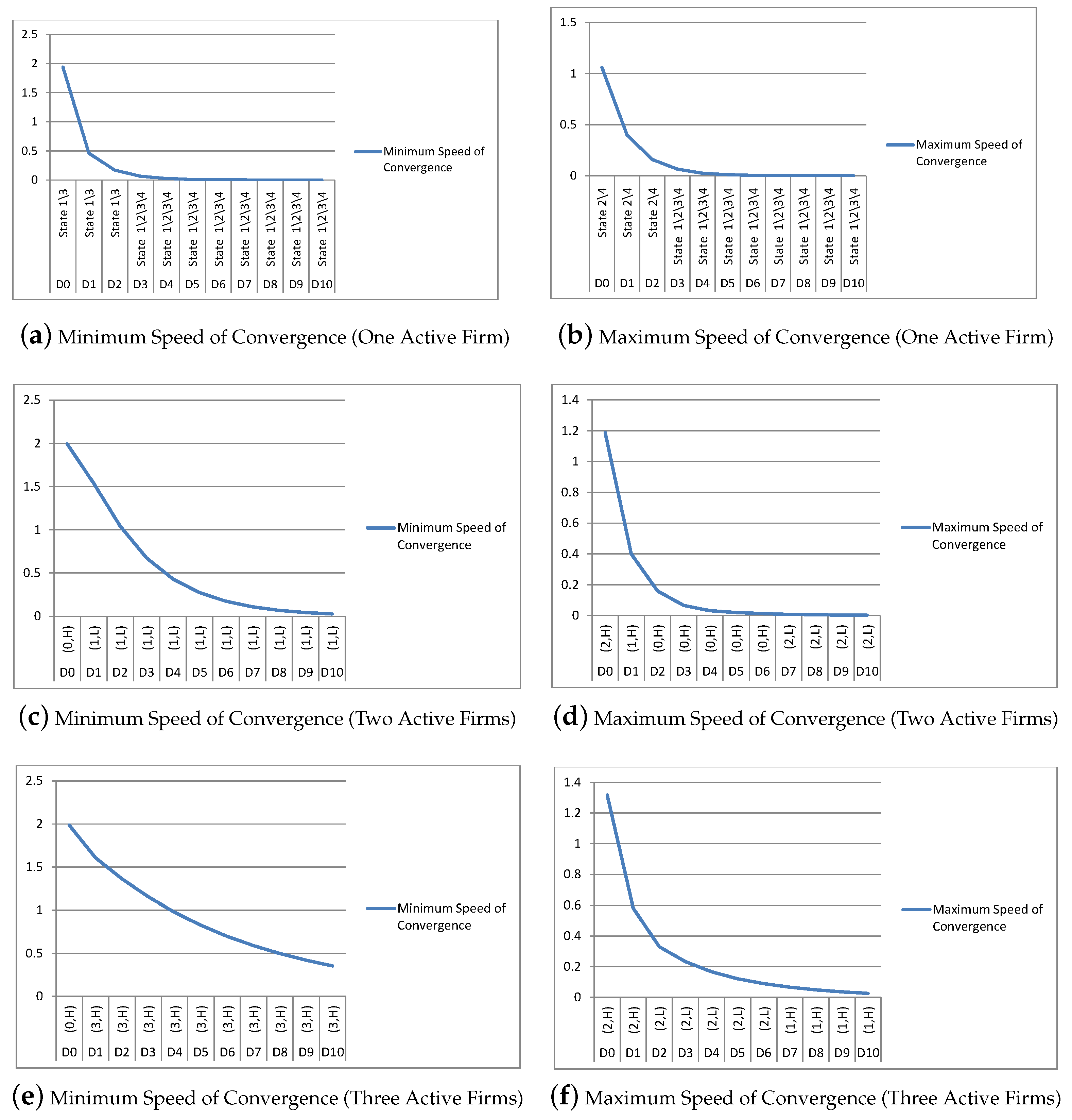
Figure 1, the D0 to D10 are calculated from the sum of absolute value of the probability for each state by the power of transition matrix from period 0 to period 10 minus the steady state probability for each state, respectively. Here, the horizontal axis indicates the initial states of the system, which have the minimum or maximum converging speed to the steady states of the system from period 0 to 10. The vertical axis means values for the minimum or maximum of converging speed to the steady states of the system during these 11 periods.
Figure 1a,b show the maximum and minimum speed of convergence to the steady state of the system for the one active firm’s case in the Cournot framework. We discover that the speed of convergence is maximum when the initial states of the system is
or
for any periods no more than three, then has indifference speed of converge with different initial states. In contrast, the initial states
or
have the minimum speed of convergence for any periods no more than three. We present the minimum and maximum speed of convergence for two active firms’ case in
Figure 1c,d. We discover the initial state of the system
has the minimum speed of convergence for any periods no less than one. As for the maximum speed of convergence, it appears in the initial state
for any periods, which is greater than 3 and less than 7.
Figure 1e,f show the maximum and minimum speed of convergence for the three active firms’ case. The initial state of the system
has the minimum speed of convergence for any periods no less than 1 and the maximum speed of convergence appears in the initial state
for any periods, which is greater than 3 and less than 7.
Setting the convergence criteria equal to the distance between the probability distribution of the state in period t and thus the probability distribution of the steady state is supposed to be less than 0.01, we conclude that only the one and two active firms’ cases are with their maximum speed of convergence in the Cournot framework. Nevertheless, the probability distribution in period t is certain to converge to the steady state, for the one-firm, two-firm, and three-firm cases with both their maximum and minimum speed, if t is large enough.
4. Conclusions
This paper elaborates the dynamic interaction in a Cournot market. In our settings, making a positioning investment can be used by a firm who would like to enter the market in the next period. The rate of success and the cost of the investment are determined by the firm’s position. In the market, all the established firms simultaneously set their quantities while the unestablished firms could not enter the market until they make an investment to establish their positions. The demand of market in our paper is symmetric and the positioning strategy of firms are asymmetric.
Our model is based on the symmetric Markov perfect Nash equilibrium (SMPNE), in which the firms make their positioning investment strategy first and then the quantity strategy. By considering the cases with one, two, and three active firms in a Cournot market, respectively, we present firm profit, consumer surplus, and total surplus, show the transition probabilities, find the steady state of the system, and discuss the speed of convergence. The dynamic uncertainty on market demand is modeled in a symmetric way while transmission probability of firms’ market position across different period is asymmetric.
This paper extends the model developed by Bloch et al. (2014) [
1] with two significant modifications. First, we assume the entry of firms is stochastic, so firms have to consider the uncertainty after making the positioning investment strategy. Second, we assume there are two levels of demand a niche market and realization of market demand is stochastic, so firms have to consider the uncertainty of the market demand given the successful investment. This work also extends the study of Lian and Zheng (2019) [
2] in which the price competition is studied. In this paper, we study the output competition in Cournot market where firms set their quantities simultaneously.
There are several possibilities to further extend our current work. First, our work focuses on the Cournot competition for the stage game, and it is worth investigating to consider the Stackelberg stage game where the firms with established positions serve as leaders while firms with unestablished positions serve as followers (Ford et al., 2019) [
33]. It is also possible to consider the sticky prices models, following Fershtman and Kamien (1987) [
8], Claudio (2000) [
9], Cellini and Lambertini (2004) [
10], Wiszniewska-Matyszkiel et al. (2015) [
11], Colombo and Labrecciosa (2019) [
12]. Second, this paper assumes that the number of firms is exogenously fixed, and it is meaningful to further study an endogenously determined market structure (Ford et al., 2020) [
33]. In addition, one may also consider (Kuang et al., 2021) [
34] of positioning investment and/or take the interdependence between market condition and positioning investment into account.


