Abstract
One class of cooperative differential games on networks is considered. It is assumed that interaction on the network is possible not only between neighboring players, but also between players connected by paths. Various cooperative optimality principles and their properties for such games are investigated. The construction of the characteristic function is proposed, taking into account the network structure of the game and the ability of players to cut off connections. The conditions under which a strong time-consistent subcore is not empty are studied. The formula for explicit calculation of the Shapley value is derived. The results are illustrated by the example of one differential marketing game.
1. Introduction
One of the current directions of research in game theory is network games. Such games explore individuals’ interactions connected through a network and whose behavior depends on their neighbors’ behavior. An overview and structuring of the main trends in network games can be found in [1,2,3,4].
The theory of differential games on networks is commonly used when the evolution of decision-making occurs continuously in time. The papers investigating applied models of differential games on networks confirm the relevance of this topic. For example, a differential game of a duopoly with network externalities is examined in [5]. Differential games with network structure in marketing are considered in [6]. An application of such games in regional cooperation is developed in [7]. Adaptation of differential games to the problem of network traffic is proposed in [8]. Cooperative differential games on networks were first considered by L. Petrosyan [9], who introduced a new type of strategies. The possibility of cutting the links with neighboring players during the game is included in these strategies. When evaluating a coalition’s worth, the classical methods assume that players who are not in this coalition minimize the coalition’s payoff. The use of the new type of strategies has led to the possibility of measuring a coalition’s worth without considering the actions of players who are not members of this coalition. Based on this, a novel form for characteristic function—named as cooperative-trajectory characteristic function—is proposed in [10]. Moreover, it satisfies the convexity property. In [11], formulas for the Shapley value and some core imputations are obtained using the new characteristic function. In this paper, we generalize the approach used in [10,11] on a more interesting case when the payoff of a player depends not only on his neighbors’ actions but also on players’ actions with whom paths in the network connect the player. This case differs essentially from one considered in [10]. In such games, the convexity of the new characteristic function depends on the structure of the network on which the game is defined.
In this paper, we consider cooperative differential games on networks defined on a given time-interval. We suppose that payoffs are transferable. Under the cooperation, we understand that players choose their strategies to maximize the sum of payoffs and then define a rule (optimality principle) on how to allocate this joint payoff between them. There are different optimality principles such as core, NM-solution, the Shapley Value, and others in classical and differential game theory. However, a serious problem arises with time-consistency and, in the case of set-valued optimality principles, also with strong time-consistency, which very often is not satisfied (see [12,13]). This makes questionable the application of the optimality principles mentioned above.
Thus, our main contributions to the literature on differential network games are the following:
- A new characteristic function for the game with interactions through paths is defined.
- It is found that the properties of such a characteristic function depend on the game’s network structure.
- A condition under which the characteristic function is convex is obtained.
- Under this condition, we prove the non-emptiness of the strong time-consistent subcore and receive explicit forms for the Shapley value and the IDP of imputations from the strong time-consistent subcore.
The paper is structured as follows. The definition of the cooperative differential game on a network is given in Section 2. In Section 3, the definition of the characteristic function based on cooperative strategies used by players from a coalition is given. As mentioned above, the basic difference from previous approaches is that, when defining the value of the characteristic function for a given coalition, it is supposed that the left out players trying to minimize the payoff of the coalition are cutting connections with players from this coalition. Based on defined characteristic function, the core is constructed, and a strong time-consistent solution as a subset of the core is proposed in Section 4. The formula for the dynamic Shapley value is derived in Section 5. As an illustrative example, a differential marketing game on the network is investigated in Section 6. For this game, the characteristic function, the strong time-consistent subset of the core, and the dynamic Shapley value are computed in explicit form.
2. Problem Formulation
Consider a class of n-person differential games with prescribed duration of T. Let be the set of players. The players are connected in a network system. A pair is called a network, where N is a set of nodes and is a given set of links. The nodes are used to represent the players. If pair , there is a link connecting players and . It is supposed that all links are undirected.
Denote the set of players directly connected to player i as .
Denote by where , the set of players connected with player by a minimal path containing exactly m edges (only paths without cycles and loops are considered) and let , for .
Every player at any instant of time can cut the connection with any other players from .
The system dynamics is given by
Here, is the state variable of player at time t and is the control variable of player . The function is continuously differentiable in and .
The payoff function of player i depends on his state variable, the state variables of players from the sets , , and his control variable. In particular, the payoff of player i is given as
The term is the instantaneous gain that player i can obtain through interaction with player and is the instantaneous gain that player i can obtain by itself. Assume that . The multiplier shows that, the farther players are in the network from player i, the less their behavior influences the payoff of this player. Suppose that functions , for are non-negative. We denote by the vector of initial conditions.
We say that we have the game if the network is defined, the system dynamics (1) and the sets of feasible controls , are given, and the players’ payoffs are determined by (2). Each player, choosing a control variable from his set of feasible controls, steers his own state according to the differential Equation (1) and seeks to maximize his objective functional (2).
Suppose that players can cooperate in order to achieve the maximum joint payoff
subject to dynamics (1).
The optimal cooperative strategies of players , for are defined as follows
The trajectory corresponding to the optimal cooperative strategies is the optimal cooperative trajectory . The maximum joint payoff can be expressed as:
subject to dynamics
To determine how to allocate the maximum total payoff among the players under an agreeable scheme, defining the characteristic function is necessary.
There are many approaches to define the characteristic function (see [14,15,16]).
In [9], for differential games on networks, it is supposed that the worth of the coalition does not take into account the actions of players from the coalition , since the worst thing they can do for the coalition S is to cut the connection with players from S. In [10], it is also proposed to find the value of the characteristic function of S on the cooperative trajectory when the players from S use cooperative strategies under the condition that the connections with players from are cut off. The characteristic function constructed in this way is easier to compute and possesses some advantageous properties. In this paper, we apply this approach to the class of games under consideration.
Let . A pair is called a subnet (subgraph) if it only has subset S of the set of vertices (players) of the original network and contains all links from L whose initial and final vertices are both within subset S. For player , denote by where , the set of players connected with player i by a minimal path in containing exactly m edges and let , for .
The worth of coalition S in the game is evaluated along the cooperative trajectory
where and are the solutions obtained in (4) and (6).
Similarly, the cooperative-trajectory characteristic function of the subgame starting at time can be evaluated as
3. Properties of the Characteristic Function
In references [10,11], the characteristic function is constructed in a similar way, but it was assumed that if the players i and j are not connected by an edge. It was shown that such characteristic function is convex. Characteristic function is called convex (or supermodular) if for any coalitions the following condition holds: . A game is called convex if its characteristic function is convex. However, in our case, additional restrictions on the network are required for the characteristic function to be convex.
Define functions that can be interpreted as instantaneous values of the characteristic function according to the following rule:
Proposition 1.
Let , . If there are no cycles in the network , then the following inequality holds for each and each :
Proof.
For simplicity, we denote
The absence of cycles in the network (tree or forest) means that there can be only one path between any two vertices. Suppose If vertex i lies on the path between some vertices in the coalition , then the path between these vertices does not exist in . Let be the set of pairs of vertices such that , , the distance between them equals m, all the vertices of the path between p and q belong to S, and i lies on this path. Then,
Since and , we have
It follows that (10) is satisfied. □
Remark 1.
Note that the presence of a cycle in the network can lead to the violation of property (10).
Indeed, the presence of a cycle in the network allows several paths between two vertices. Let us assume that there are two paths with the length r between vertices and . Suppose that all vertices from the first path belong to , and vertex i lies on this path. Assume also that the second path contains vertices from and vertex i does not lie on this path.
Note that there exists a path between p and q in , but there is no path between these vertices in , since the first path goes through player i who is no longer in the coalition and the second path does not belong to . Then, there is a term in the right-hand side of (12).
There are two paths with the length r between vertices p and q in . One of them passes through vertex i and the other does not. Thus, there exists path between p and q in . This means that, on the right-hand side of (11), there is no term corresponding to the vertices p and q.
Thus, if is large enough, inequality (10) will not hold.
Corollary 1.
Proof.
It is shown that, for each , , and each , the following inequality holds:
Integrating both sides of this inequality with respect to t, we have for each , each , , and each
The absence of cycles guarantees the convexity of the characteristic function. However, even if there are cycles in the network, the characteristic function defined according to a given rule (7) and (8) may be convex for some parameter values. Therefore, the existing formula (7) for the characteristic function is relevant not only for networks without cycles.
4. Strong Time-Consistent Subcore
The next problem to define a cooperative solution is to determine an allocation rule to distribute among the players their maximum joint payoff. We again assume that there are no cycles in the network .
The set of all imputations in the game , , is given by
Definition 1
([17]). The core of the game is the subset of the imputation set , such that
Similarly, for every denote by the set of all imputations and by the core in the subgame along the cooperative trajectory.
The convexity of the characteristic function (7) and (8), which is proved above, guarantees that the core is not empty for every [17].
The time consistency of cooperative solutions is an important issue when considering dynamic games. Suppose the optimality principle chosen by the players contains a set of imputations. In that case, as the game evolves along the cooperative trajectory , the players can deviate from the imputation chosen in the initial time for any other imputation in that optimality principle. Will it lead to the payment rule selected in the game corresponding to the initial optimality principle? This is true only if the cooperative solution is strong time-consistent. This property of cooperation solution was introduced by L. Petrosyan [13]. Let us show that there is a subset of the core in the class of games under consideration, which is strong time-consistent.
Definition 2
(see [18]). A function , is the imputation distribution procedure (IDP) for imputation , if
Definition 3
(see [13]). An optimality principal is called strong time-consistent if
- 1.
- .
- 2.
- For each there exists an IDP , , such that , and
For , , the symbol ⊕ means the following: .
In [19], a method for constructing a strong time-consistent subset of the core is proposed. Furthermore, conditions under which such a subset exists are obtained. In this paper, we implement this approach for the class of games under consideration, taking into account the peculiarities of the definition of the characteristic function.
Using the functions introduced in (9), we define for each as the set of functions such that
Note that, if we consider as a characteristic function of the stationary game, then is an imputation in this game and coincides with its core. Taking into account the fulfillment of property (10), we can conclude that, for each , the set is not empty in the considered class of games since the characteristic function in each moment t is convex [17].
To prove that is an IDP in the initial differential game , let us consider . Now, we define in the following way
According to (17),
Then,
and
which proves that . is an IDP for this imputation. Similarly, it can be proved that, for every vector , defined by
is an imputation in .
Denote by the set of all imputations , specified by Equation (20) for all .
Proposition 2.
In the class of games under consideration, the sets are non-empty for every and .
Proof.
The sets are non-empty for each because functions are convex for each . Then, are non-empty for each .
Now, we prove that .
Let . Then, for , there exists an IDP , such that
Then,
From (22), it follows that the imputation belongs to the core for each . This means that for each . □
Proposition 3.
is a strong time-consistent optimality principle in the game .
Proof.
The proof follows directly from Theorem 5.1 in [19]. □
Consider also a rule for constructing some IDP from the set .
Denote by the set of pairs , where , , the distance between k and l equals m, and vertex i belongs to the path between k and l (i can coincide with k or l). Let be the set of pairs , where , , with the distance between k and l equal to m, all vertices from this path belonging to S, and vertex i lying on the path between k and l.
For each pair of vertices , , we denote by the set of vectors ), such that , , for each . Here, we assume the length of the path between p and q equals m (for each vertex , , belonging to the path between p and q, the coefficient is given).
Proposition 4.
In the class of games under consideration, the IDP defined by the Equation (23) belongs to the set for any for each pair of vertices ,
Proof.
This concludes the proof. □
5. The Shapley Value
Consider also the problem of constructing the Shapley value (see [20]) in differential games on networks. It turned out that using the characteristic function (7) in the considered class of games, the construction of the Shapley value does not require the calculation of the characteristic function of every . Proposition 5 demonstrates this specific result.
Proposition 5.
Proof.
The formula for the Shapley value [20] is as follows
Consider the term . This is the value that the coalition S loses when a player i leaves it. This value consists of
- is the payoff of player i that he can obtain by itself.
- is the payoff that player i receives from interaction with players from .
- is the payoff that players from receive from interaction with player i.
- are the payoffs that players p and q receive from interaction with each other, where p and q are such vertices from that there exists a path with the length m between them in S, and player i lies on this path (since there is no path in between p and q, because player i leaves the set S).
Rewrite the values from the last three items into one summand using the definition of sets :
Consider two fixed players k and l with the length of the path between them equal to m. These two vertices (players), together with all vertices (players) from the path between them, are included in coalitions of power s. Then,
where
Then,
This concludes the proof. □
Remark 2.
belongs to the strong time-consistent subcore. This can be verified by choosing an IDP for it, constructed according to (23) with all coefficients equal to .
6. One Cooperative Differential Network Marketing Game
As an illustrative example, we consider a simple model of network marketing. There are n distributors (players) selling the same product or brand. Let denote the sales rate of player i. The sales rate dynamics of player i evolves according to the accumulation equation
where is the promotional effort of distributor i, .
We assume that each player’s payoff depends on their own sales and those of other distributors. First, we consider the general case where a player’s payoff depends on all participants’ sales, taking into account the distance between players on the network. Then, we apply the obtained solution to a multi-level marketing model on a directed network. The directions of arcs are supposed to indicate the hierarchy between players. In this case, distributors can only benefit from down-line distributors.
If each agent extracts linear utility from his own sales and sales of other participants and the cost function has a quadratic form, then the objective functions are given by
Here, is the instantaneous gain that player i can obtain by himself, is the instantaneous gain that player i obtains through interaction with player , and is a cost function of agent i. Parameter indicates the percentage of sales of player j that player i receives.
Suppose that the game is played in a cooperative scenario and players have the opportunity to cooperate in order to achieve maximum total payoff:
To define the cooperative strategies, we use the Bellman dynamic programming technique. We denote by the Bellman function in a subgame starting at the moment t from :
The Hamilton–Jacobi–Bellman (HJB) equation has the following expression:
The solution of (34) is found in the form
Substituting it into (34), we have the following system of differential equations for and B(t):
The solution of (37) is the following
where .
Then, the optimal cooperative strategies have the form
The optimal cooperative trajectory is
The value function for the cooperative joint payoff of all n players can be obtained as
According to (7), the characteristic function becomes
Consider now the numeric example for the case of multi-level marketing game. This model assumes that the graph is directed. The direction of edge from player i to player j means that player i has recruited player j.
Figure 1 shows the structure of the network in the game. It is assumed that distributors can only benefit from down-line distributors. In the framework of the considered example of network marketing, this means that .
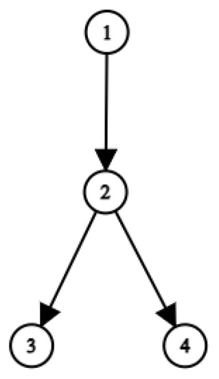
Figure 1.
A four-player multi-level marketing game.
We assume the following values of the remaining parameters: , , , , , , , , , , , , , , .
According to Proposition 5, the Shapley value has the form
Thus, to obtain the Shapley value, it is not necessary to calculate all the values of the characteristic function; it is enough to find the following quantities:
Then,
To construct IDP from , we use a set of coefficients that satisfy the system:
Then, the formulas for IDP have the form:
Choosing , we obtain the IDP for the Shapley Value.
Finally, we show the graphical representation of the obtained solutions. Expressing and passing to the system of inequalities with three variables (15) to find the core, we plot the resulting area in Figure 2. The Shapley value (red color) and imputations from the strong time-consistent subcore, calculated according to (23) (blue color), are also indicated in Figure 2.
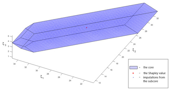
Figure 2.
Cooperative solutions in a four-player multi-level marketing game.
The example considered in Section 6 illustrates a possible application of the proposed model and shows how to distribute the joint payoff between the players connected by the network. This example also shows the possibility of applying the obtained solutions to the case of a directed graph.
7. Conclusions
One class of cooperative differential games on networks is investigated. It is assumed that each player’s payoff depends not only on his neighbors’ actions but also on players’ actions with whom paths in the network connect the player. A novel form for characteristic function in such games is proposed. It is shown that the convexity of this characteristic function not always takes place and essentially depends on the structure of the network on which the game is defined. It is proved that, if the network has no cycles, then the characteristic function is convex and the strong time-consistent subcore is not empty. The formula for explicit calculation of the Shapley value is derived. An algorithm for the construction of IDP, corresponding to imputations from the strong time-consistent subcore is given. An illustrative example demonstrating this result is considered.
Further research can be done on cooperative differential games on networks. It will be interesting to use the approach based on cooperative trajectory characteristic functions to differential games defined on general networks containing cycles. It seems that, in this case, the convexity of the corresponding characteristic function will not take place, but the existence of the core could be proved, and the dynamic Shapley value could be calculated in explicit form. It would also be interesting to obtain such values of for which the characteristic function turns out to be convex even in the presence of cycles in the network.
Author Contributions
Conceptualization, L.P.; Formal analysis, L.P. and A.T.; Investigation, A.T.; Methodology, L.P. and A.T.; Project administration, A.T.; Supervision, L.P.; Validation, L.P. and A.T.; and Writing—original draft, L.P. and A.T. All authors have read and agreed to the published version of the manuscript.
Funding
The work by L. Petrosyan was supported by Russian Science Foundation (grant N 17-11-01079).
Institutional Review Board Statement
Not applicable.
Informed Consent Statement
Not applicable.
Data Availability Statement
Not applicable.
Conflicts of Interest
The authors declare no conflict of interest.
References
- Mazalov, V.; Chirkova, J.V. Networking Games: Network Forming Games and Games on Networks; Academic Press: Cambridge, MA, USA, 2019. [Google Scholar]
- Jackson, M.O.; Zenou, Y. Games on Networks. Handbook of Game Theory; Young, P., Zamir, S., Eds.; Elsevier Science: Amsterdam, The Netherlands, 2014; Volume 4. [Google Scholar]
- Sedakov, A. Dynamic Network Games. Ph.D. Thesis, St. Petersburg State University, St. Petersburg, Russia, 2020. [Google Scholar]
- Gao, H.; Pankratova, Y. Cooperation in Dynamic Network Games. Contrib. Game Theory Manag. 2017, 10, 42–67. [Google Scholar]
- Meza, M.A.G.; Lopez-Barrientos, J.D. A differential game of a duopoly with network externalities. In Recent Advances in Game Theory and Applications; Petrosyan, L.A., Mazalov, V.V., Eds.; Springer: Cham, Switzerland, 2016. [Google Scholar] [CrossRef]
- Gromova, E.; Malakhova, A. Solution of Differential Games with Network Structure in Marketing. In Frontiers of Dynamic Games. Static & Dynamic Game Theory: Foundations & Applications; Petrosyan, L.A., Mazalov, V.V., Zenkevich, N.A., Eds.; Birkäuser: Cham, Switzerland, 2020. [Google Scholar]
- Petrosyan, L.; Yeung, D. Shapley value for differential network games: Theory and application. J. Dyn. Games 2020. [Google Scholar] [CrossRef]
- Wie, B.W. A Differential Game Model of Nash Equilibrium on a Congested Traffic Network. Networks 1993, 23, 557–565. [Google Scholar] [CrossRef]
- Petrosyan, L.A. Cooperative Differential Games on Networks. Trudy Inst. Mat. I Mekh. UrO RAN 2010, 16, 143–150. [Google Scholar]
- Petrosyan, L.; Yeung, D. Construction of Dynamically Stable Solutions in Differential Network Games. In Stability, Control and Differential Games. Lecture Notes in Control and Information Sciences— Proceedings; Tarasyev, A., Maksimov, V., Filippova, T., Eds.; Springer: Cham, Switzerland, 2020. [Google Scholar] [CrossRef]
- Tur, A.; Petrosyan, L. Cooperative optimality principles in differential games on networks. Math. Theory Appl. 2020, 12, 93–111. [Google Scholar]
- Yeung, D.W.K.; Petrosyan, L.A. Subgame Consistent Cooperation; Springer Science and Business Media LLC: Singapore, 2016. [Google Scholar]
- Petrosyan, L.A. Strong Time-Consistent Differential Optimality Principles. Vestn. Leningrad. Univ. 1993, 4, 35–40. [Google Scholar]
- Von Neumann, J.; Morgenstern, O. Theory of Games and Economic Behavior; Princeton University Press: Princeton, NJ, USA, 1953. [Google Scholar]
- Gromova, E.; Petrosyan, L. On an approach to constructing a characteristic function in cooperative differential games. Autom. Remote Control 2017, 78, 98–118. [Google Scholar] [CrossRef]
- Gromova, E.; Marova, E.; Gromov, D. A substitute for the classical Neumann-Morgenstern characteristic function in cooperative differential games. J. Dyn. Games 2020, 7, 105–122. [Google Scholar] [CrossRef]
- Shapley, L.S. Cores of convex games. Int. J. Game Theory 1971, 1, 11–26. [Google Scholar] [CrossRef]
- Petrosyan, L.A.; Danilov, N.N. Stable Solutions in Nonantagonistic Differential Games with Transferable Payoffs. Vestn. Leningrad. Univ. 1979, 1, 52–79. [Google Scholar]
- Petrosian, O.L.; Gromova, E.V.; Pogozhev, S.V. Strong Time-Consistent Subset of the Core in Cooperative Differential Games with Finite Time Horizon. Autom. Remote Control 2018, 79, 1912–1928. [Google Scholar] [CrossRef]
- Shapley, L.S. A value for n-person games. In Contributions to the Theory of Games; Annals of Mathematics Studies; Princeton University Press: Princeton, NJ, USA, 1953; Volume 2, p. 28. [Google Scholar]
Publisher’s Note: MDPI stays neutral with regard to jurisdictional claims in published maps and institutional affiliations. |
© 2021 by the authors. Licensee MDPI, Basel, Switzerland. This article is an open access article distributed under the terms and conditions of the Creative Commons Attribution (CC BY) license (https://creativecommons.org/licenses/by/4.0/).