
Rule-Based EEG Classifier Utilizing Local Entropy of Time–Frequency Distributions


Abstract
1. Introduction
2. Materials and Methods
2.1. Signal Analysis in the Time–Frequency Domain
- Identification of signal characteristics (such as time and frequency variations and the number of signal components);
- Extracting components from their mixtures and background noise;
- Ability to synthesize extracted components in the time domain;
- Analysis of features (such as instantaneous amplitude, frequency, and bandwidth of each component).
2.1.1. Spectrogram
2.1.2. Wigner–Ville Distribution (WVD)
2.1.3. The Quadratic Class of Time–Frequency Distributions
2.2. Measuring TFDs’ Information Content Using the Global Rényi Entropy
The Local or Short-Term Rényi Entropy (STRE)
2.3. Instantaneous Frequency Estimation
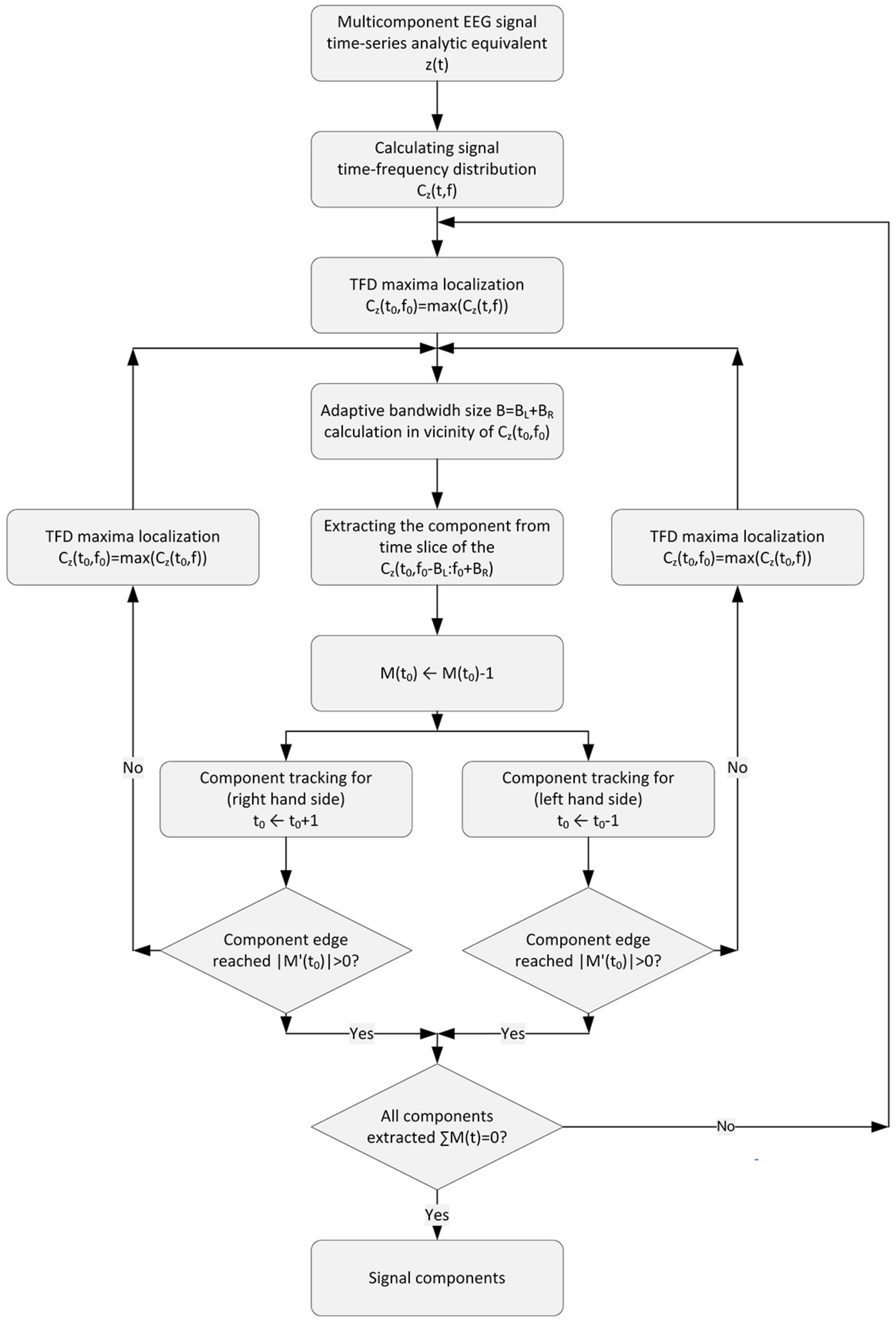
2.4. Component Extraction Procedure
2.5. Real data
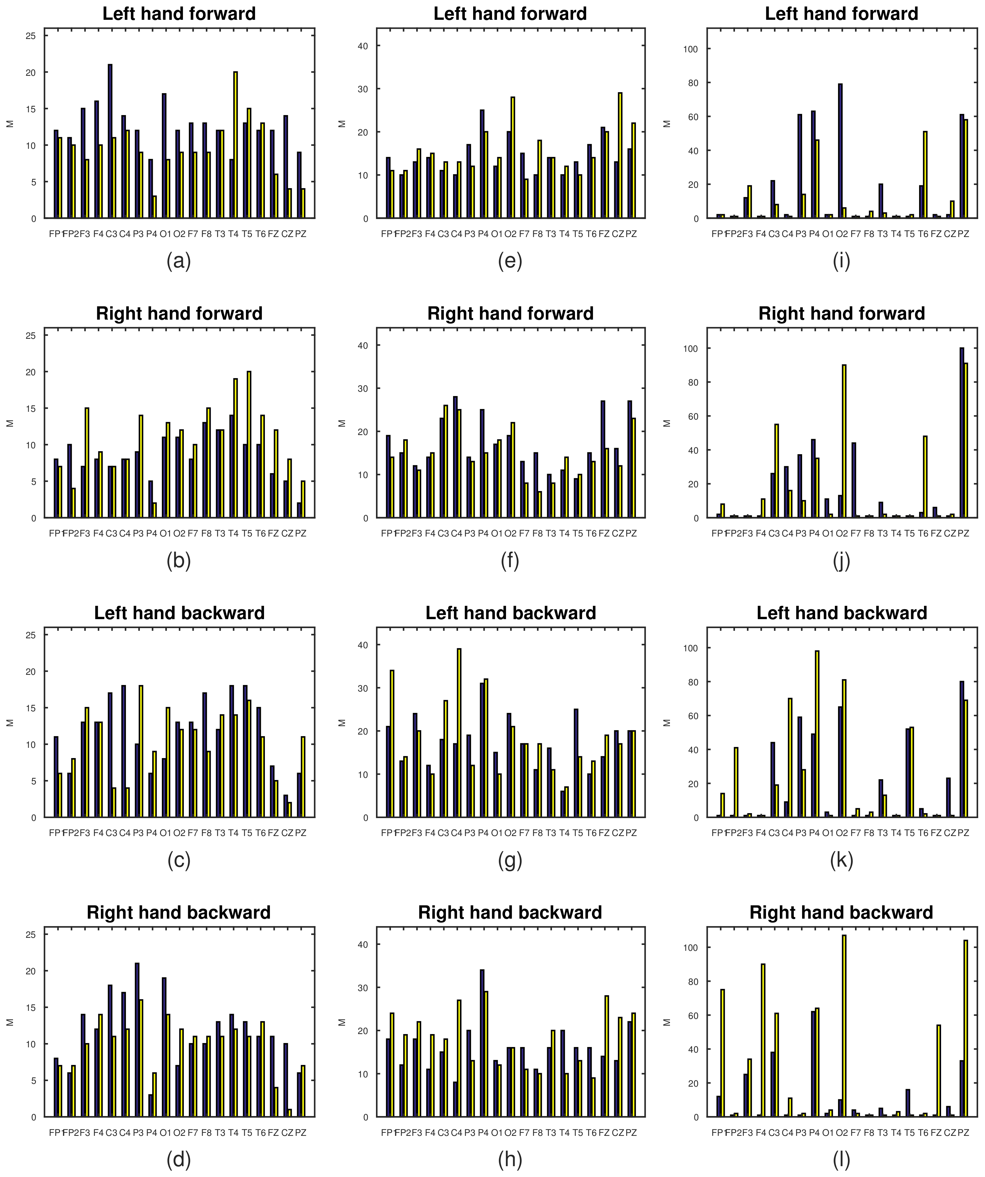
3. Results
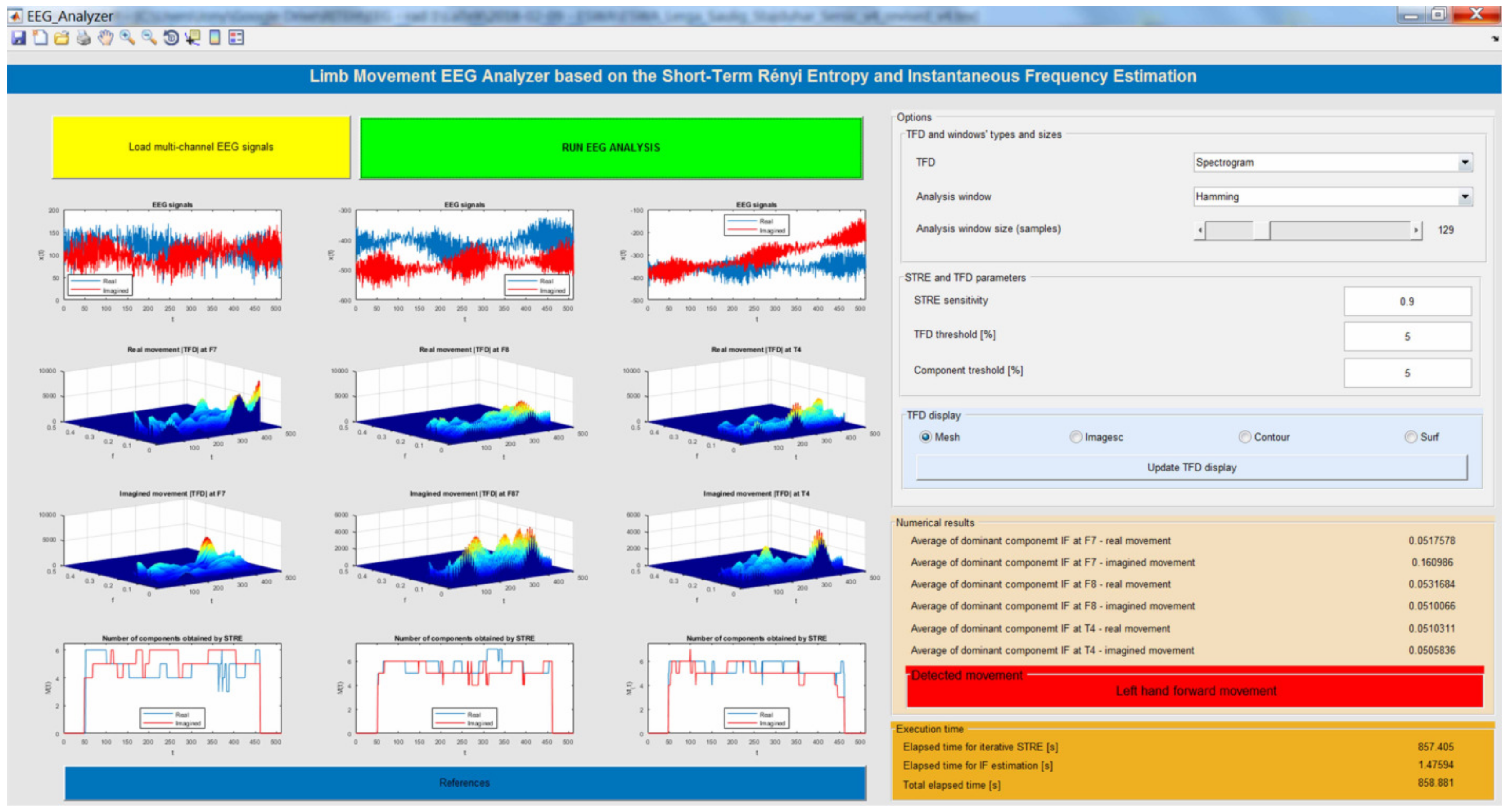
EEG Analyzer Implemented in a Virtual Computer Instrument
- Load multi-channel EEG signals: The user imports multi-channel EEG records as a MAT file (for real and imagined limb movements), which are then shown in the first row of the proposed instrument.
- Run EEG analysis: By clicking on this button, the EEG analysis is started by employing STRE- and IF-based algorithms.
- Displaying results: The results are shown in twelve figures as follows. The first row of figures (from top to bottom) show EEG time series at F7, F8, and T4. The second row of figures show the TFDs of the EEGs of real limb movements, followed by the TFDs of the EEG signals of imagined movements, which are given in the third row. The fourth row of figures present the instantaneous number of EEG components obtained using the STRE for both real and imagined movements.
- Numerical results: The application provides numerical results in terms of the average of the dominant EEG component IFs at F7, F8, and T4 for the real and imagined limb movements. Based on these dominant components’ IFs, the analyzed limb movements are estimated. In addition, the instrument shows elapsed time for both the STRE and IF estimations, as well as the total elapsed time for overall EEG analysis.
- Selecting TFD and windows’ sizes and types: The user is allowed to choose a TFD from the provided list of TFDs, and depending on the chosen TFD, they are allowed to set the analyzing window width and type (Hamming, Hanning, rectangular, triangular, Gauss, and Kaiser).
- STRE and TFD parameters: In addition, prior to running EEG analysis, the user is allowed to select values of the STRE sensitivity parameter, the TFD threshold for reducing noise and low-energy cross-terms, and the component extraction threshold.
- TFD display options: The proposed instrument allows display of the TFDs as imagesc (TFD is displayed as an image), contour (TFD values are treated as heights above a plan), mesh (TFD is treated as colored parametric mesh), and surf (plots colored parametric surface).
- References: By clicking on this button, related papers and previous works of the authors that led to the development of the proposed instrument are given.
4. Discussion
5. Conclusions
Author Contributions
Funding
Institutional Review Board Statement
Informed Consent Statement
Data Availability Statement
Conflicts of Interest
References
- Van Hoey, G.; Philips, W.; Lemahieu, I. Time-frequency analysis of EEG signals. In Proceedings of the 8th Workshop on Circuits, Systems and Signal Processing, Mierlo, The Netherlands, 27–28 November 1997; pp. 631–636. [Google Scholar]
- Diykh, M.; Li, Y.; Wen, P. Classify Epileptic EEG Signals Using Weighted Complex Networks Based Community Structure Detection. Expert Syst. Appl. 2017, 90, 87–100. [Google Scholar] [CrossRef]
- Del Rincon, J.M.; Santofimia, M.J.; del Toro, X.; Barba, J.; Romero, F.; Navas, P.; Lopez, J.C. Non-linear classifiers applied to EEG analysis for epilepsy seizure detection. Expert Syst. Appl. 2017, 86, 99–112. [Google Scholar] [CrossRef]
- Nakisa, B.; Rastgoo, M.N.; Tjondronegoro, D.; Chandran, V. Evolutionary computation algorithms for feature selection of EEG-based emotion recognition using mobile sensors. Expert Syst. Appl. 2018, 93, 143–155. [Google Scholar] [CrossRef]
- Peng, A. Research on The EEG Signal Denoising Method Based on Improved Wavelet Transform. Int. J. Digit. Content Technol. Appl. 2013, 7, 154–163. [Google Scholar]
- Gaur, P.; Pachori, R.B.; Wang, H.; Prasad, G. A multi-class EEG-based BCI classification using multivariate empirical mode decomposition based filtering and Riemannian geometry. Expert Syst. Appl. 2018, 95, 201–211. [Google Scholar] [CrossRef]
- Gaur, P.; Pachori, R.B.; Wang, H.; Prasad, G. A multivariate empirical mode decomposition based filtering for subject independent BCI. In Proceedings of the 27th Irish Signals and Systems Conference, Derry, UK, 21–22 June 2016; pp. 1–7. [Google Scholar]
- Gaur, P.; Pachori, R.B.; Wang, H.; Prasad, G. Enhanced motor imagery classification in EEG-BCI using multivariate EMD based filtering and CSP features. In International Brain-Computer Interface (BCI) Meeting 2016; BCI Society: Utrecht, The Netherlands, 2016. [Google Scholar]
- Speckmann, E.J.; Elger, C.E.; Gorji, A. Niedermeyer’s Electroencephalography; Chapter Neurophysiologic Basis of EEG and DC Potentials; Lippincott Williams and Wilkins: Philadelphia, PA, USA, 2011; pp. 1–15. [Google Scholar]
- Sharma, M.; Dhere, A.; Pachori, R.B.; Acharya, U.R. An automatic detection of focal EEG signals using new class of time–frequency localized orthogonal wavelet filter banks. Knowl. Based Syst. 2017, 118, 217–227. [Google Scholar] [CrossRef]
- Aboalayon, K.A.I.; Faezipour, M.; Almuhammadi, W.S.; Moslehpour, S. Sleep Stage Classification Using EEG Signal Analysis: A Comprehensive Survey and New Investigation. Entropy 2016, 18, 272. [Google Scholar] [CrossRef]
- Hassan, A.R.; Subasi, A. A decision support system for automated identification of sleep stages from single-channel EEG signals. Knowl. Based Syst. 2017, 128, 115–124. [Google Scholar] [CrossRef]
- Rosenblatt, M.; Figliola, A.; Paccosi, G.; Serrano, E.; Rosso, O.A. A Quantitative Analysis of an EEG Epileptic Record Based on MultiresolutionWavelet Coefficients. Entropy 2014, 16, 5976–6005. [Google Scholar] [CrossRef]
- Bhati, D.; Pachori, R.B.; Gadre, V.M. A novel approach for time–frequency localization of scaling functions and design of three-band biorthogonal linear phase wavelet filter banks. Digit. Signal Process. 2017, 69, 309–322. [Google Scholar] [CrossRef]
- Bhati, D.; Sharma, M.; Pachori, R.B.; Gadre, V.M. Time–frequency localized three-band biorthogonal wavelet filter bank using semidefinite relaxation and nonlinear least squares with epileptic seizure EEG signal classification. Digit. Signal Process. 2017, 62, 259–273. [Google Scholar] [CrossRef]
- Sharma, R.; Pachori, R.B. Classification of epileptic seizures in EEG signals based on phase space representation of intrinsic mode functions. Expert Syst. Appl. 2015, 42, 1106–1117. [Google Scholar] [CrossRef]
- Pachori, R.B. Discrimination between ictal and seizure-free EEG signals using empirical mode decomposition. Res. Lett. Signal Process. 2008, 2008, 1–5. [Google Scholar] [CrossRef]
- D’Avanzo, C.; Tarantino, V.; Bisiacchi, P.S.; Sparacino, G. A wavelet Methodology for EEG Time-frequency Analysis in a Time Discrimination Task. Int. J. Bioelectromagn. 2009, 11, 185–188. [Google Scholar]
- Zhang Xizheng, Y.L.; Weixiong, W. Wavelet Time-frequency Analysis of Electro-encephalogram (EEG) Processing. Int. J. Adv. Comput. Sci. Appl. 2010, 1, 1–5. [Google Scholar] [CrossRef]
- Boashash, B. Time-Frequency Signal Analysis and Processing: A Comprehensive Reference; Academic Press: Cambridge, MA, USA, 2015. [Google Scholar]
- Sucic, V.; Lerga, J.; Boashash, B. Multicomponent noisy signal adaptive instantaneous frequency estimation using components time support information. IET Signal Process. 2014, 8, 277–284. [Google Scholar] [CrossRef]
- Lerga, J.; Sucic, V.; Boashash, B. An Efficient Algorithm for Instantaneous Frequency Estimation of Nonstationary Multicomponent Signals in Low SNR. EURASIP J. Adv. Signal Process. 2011, 2011, 1–16. [Google Scholar] [CrossRef]
- Lerga, J.; Sucic, V. Nonlinear IF Estimation Based on the Pseudo WVD Adapted Using the Improved Sliding Pairwise ICI Rule. IEEE Signal Process. Lett. 2009, 16, 953–956. [Google Scholar] [CrossRef]
- Sharma, M.; Achuth, P.V.; Pachori, R.B.; Gadre, V.M. A parametrization technique to design joint time–frequency optimized discrete-time biorthogonal wavelet bases. Signal Process. 2017, 135, 107–120. [Google Scholar] [CrossRef]
- Sharma, M.; Dhere, A.; Pachori, R.B.; Gadre, V.M. Optimal duration-bandwidth localized antisymmetric biorthogonal wavelet filters. Signal Process. 2017, 134, 87–99. [Google Scholar] [CrossRef]
- Sharma, M.; Bhati, D.; Pillai, S.; Pachori, R.B.; Gadre, V.M. Design of Time-Frequency Localized Filter Banks: Transforming Non-convex Problem into Convex Via Semidefinite Relaxation Technique. Circuits Syst. Signal Process. 2016, 35, 3716–3733. [Google Scholar] [CrossRef]
- Lerga, J.; Sucic, V. An instantaneous frequency estimation method based on the improved sliding pair-wise ICI rule. In Proceedings of the 10th International Conference on Information Science, Signal Processing and their Applications (ISSPA 2010), Kuala Lumpur, Malaysia, 10–13 May 2010; pp. 161–164. [Google Scholar]
- Sun, M.; Scheuer, M.L.; Qian, S.; Baumann, S.B.; Adelson, P.D.; Sclabassi, R.J. Time-frequency analysis of high-frequency activity at the start of epileptic seizures. In Proceedings of the 19th Annual International Conference of the IEEE Engineering in Medicine and Biology Society. ‘Magnificent Milestones and Emerging Opportunities in Medical Engineering’ (Cat. No.97CH36136), Chicago, IL, USA, 30 October–2 November 1997; Volume 3, pp. 1184–1187. [Google Scholar]
- Tzallas, A.T.; Tsipouras, M.G.; Fotiadis, D.I. The Use of Time-Frequency Distributions for Epileptic Seizure Detection in EEG Recordings. In Proceedings of the 29th Annual International Conference of the IEEE Engineering in Medicine and Biology Society, Lyon, France, 23–26 August 2007; pp. 3–6. [Google Scholar]
- Sharma, M.; Pachori, R.B.; Acharya, U.R. A new approach to characterize epileptic seizures using analytic time-frequency flexible wavelet transform and fractal dimension. Pattern Recognit. Lett. 2017, 94, 172–179. [Google Scholar] [CrossRef]
- Tzallas, A.T.; Tsipouras, M.G.; Fotiadis, D.I. Automatic Seizure Detection Based on Time-frequency Analysis and Artificial Neural Networks. Comput. Intell. Neurosci. 2007, 2007, 18:1–18:13. [Google Scholar] [CrossRef] [PubMed]
- Tzallas, A.T.; Tsipouras, M.G.; Fotiadis, D.I. Epileptic Seizure Detection in EEGs Using Time-Frequency Analysis. IEEE Trans. Inf. Technol. Biomed. 2009, 13, 703–710. [Google Scholar] [CrossRef] [PubMed]
- Martínez-Vargas, J.D.; Avendaño-Valencia, L.D.; Giraldo, E.; Castellanos-Dominguez, G. Comparative analysis of time frequency representations for discrimination of epileptic activity in EEG signals. In Proceedings of the 2011 5th International IEEE/EMBS Conference on Neural Engineering, Cancun, Mexico, 27 April–1 May 2011; pp. 148–151. [Google Scholar]
- Subasi, A.; Gursoy, M.I. EEG signal classification using PCA, ICA, LDA and support vector machines. Expert Syst. Appl. 2010, 37, 8659–8666. [Google Scholar] [CrossRef]
- Awal, M.A.; Khlif, M.S.; Dong, S.; Azemi, G.; Colditz, P.; Boashash, B. Detection of Neonatal EEG Burst-Suppression Using Time-Frequency Matching Pursuit. In Proceedings of the Australian Biomedical Engineering Conference (ABEC), Melbourne, Australia, 22–25 November 2015. [Google Scholar]
- Rankine, L.; Stevenson, N.; Mesbah, M.; Boashash, B. A Nonstationary Model of Newborn EEG. IEEE Trans. Biomed. Eng. 2007, 54, 19–28. [Google Scholar] [CrossRef]
- Hamid Hassanpour, M.M.; Boashash, B. Time–frequency based newborn EEG seizure detection using low and high frequency signatures. Physiol. Meas. 2004, 25, 935–944. [Google Scholar] [CrossRef]
- Boashah, B.; Mesbah, M. A time-frequency approach for newborn seizure detection. IEEE Eng. Med. Biol. Mag. 2001, 20, 54–64. [Google Scholar] [CrossRef]
- Omidvarnia, A.H.; Mesbah, M.; Khlif, M.S.; O’Toole, J.M.; Colditz, P.B.; Boashash, B. Kalman filter-based time-varying cortical connectivity analysis of newborn EEG. In Proceedings of the 2011 Annual International Conference of the IEEE Engineering in Medicine and Biology Society, Boston, MA, USA, 30 August–3 September 2011; pp. 1423–1426. [Google Scholar]
- Omidvarnia, A.; Mesbah, M.; O’Toole, J.M.; Colditz, P.; Boashash, B. Analysis of the time-varying cortical neural connectivity in the newborn EEG: A time-frequency approach. In Proceedings of the International Workshop on Systems, Signal Processing and their Applications (WOSSPA), Tipaza, Algeria, 9–11 May 2011; pp. 79–182. [Google Scholar]
- Hassanpour, H.; Boashash, B. A Time-Frequency Approach For EEG Spike Detection. Iran. J. Energy Environ. 2011, 2, 390–395. [Google Scholar] [CrossRef][Green Version]
- Powell, G.E.; Percival, I.C. A spectral entropy method for distinguishing regular and irregular motion of Hamiltonian systems. J. Phys. A Math. Gen. 1979, 12, 2053–2071. [Google Scholar] [CrossRef]
- Rosenblatt, M.; Serrano, E.; Figliola, A. An Entropy Based in Wavelet Leaders to Quantify the Local Regularity of a Signal and its Application to Analize the Dow Jones Index. Int. J. Wavelets Multiresolution Inf. Process. 2012, 10, 1250048. [Google Scholar] [CrossRef]
- Jaffard, S. Oscillation spaces: Properties and applications to fractal and multifractal functions. J. Math. Phys. 1998, 39, 4129–4141. [Google Scholar] [CrossRef]
- Bhattacharyya, A.; Pachori, R.B.; Upadhyay, A.; Acharya, U.R. Tunable-Q Wavelet Transform Based Multiscale Entropy Measure for Automated Classification of Epileptic EEG Signals. Appl. Sci. 2017, 7, 385. [Google Scholar] [CrossRef]
- Bhattacharyya, A.; Pachori, R.B.; Acharya, U.R. Tunable-Q Wavelet Transform Based Multivariate Sub-Band Fuzzy Entropy With Application to Focal EEG Signal Analysis. Entropy 2017, 19, 99. [Google Scholar] [CrossRef]
- Acharya, U.R.; Yanti, R.; Zheng, J.W.; Krishnan, M.M.R.; Tan, J.H.; Martis, R.J.; Lim, C.M. Automated Diagnosis of Epilepsy Using CWT, HOS and Texture Parameters. Int. J. Neural Syst. 2013, 23, 1350009:1–1350009:15. [Google Scholar] [CrossRef] [PubMed]
- Bhattacharyya, S.; Khasnobish, A.; Chatterjee, S.; Konar, A.; Tibarewala, D.N. Performance analysis of LDA, QDA and KNN algorithms in left-right limb movement classification from EEG data. In Proceedings of the 2010 International Conference on Systems in Medicine and Biology, Kharagpur, India, 16–18 December 2010; pp. 126–131. [Google Scholar]
- Bhattacharyya, S.; Khasnobish, A.; Konar, A.; Tibarewala, D.N.; Nagar, A.K. Performance analysis of left/right hand movement classification from EEG signal by intelligent algorithms. In Proceedings of the 2011 IEEE Symposium on Computational Intelligence, Cognitive Algorithms, Mind, and Brain (CCMB), Paris, France, 11–15 April 2011; pp. 1–8. [Google Scholar]
- Caracillo, R.C.; Castro, M.C.F. Classification of executed upper limb movements by means of EEG. In Proceedings of the 2013 ISSNIP Biosignals and Biorobotics Conference: Biosignals and Robotics for Better and Safer Living (BRC), Rio de Janeiro, Brazil, 18–20 February 2013; pp. 1–6. [Google Scholar]
- Shiman, F.; López-Larraz, E.; Sarasola-Sanz, A.; Irastorza-Landa, N.; Spüler, M.; Birbaumer, N.; Ramos-Murguialday, A. Classification of different reaching movements from the same limb using EEG. J. Neural Eng. 2017, 14, 046018. [Google Scholar] [CrossRef] [PubMed]
- Waldert, S.; Preissl, H.; Demandt, E.; Braun, C.; Birbaumer, N.; Aertsen, A.; Mehring, C. Hand movement direction decoded from MEG and EEG. J. Neurosci. 2008, 28, 1000–1008. [Google Scholar] [CrossRef]
- Sanes, J.; Donoghue, J.; Thangaraj, V.; Edelman, R.; Warach, S. Shared neural substrates controlling hand movements in human motor cortex. Science 1995, 268, 1775–1777. [Google Scholar] [CrossRef]
- Yong, X.; Menon, C. EEG classification of different imaginary movements within the same limb. PLoS ONE 2015, 10, e0121896. [Google Scholar]
- Shiman, F.; Irastorza-Landa, N.; Sarasola-Sanz, A.; Spüler, M.; Birbaumer, N.; Ramos-Murguialday, A. Towards decoding of functional movements from the same limb using EEG. In Proceedings of the 2015 37th Annual International Conference of the IEEE Engineering in Medicine and Biology Society (EMBC), Milan, Italy, 25–29 August 2015; pp. 1922–1925. [Google Scholar]
- Planelles, D.; Hortal, E.; Costa, A.; Úbeda, A.; Iáez, E.; Azorín, J.M. Evaluating classifiers to detect arm movement intention from EEG signals. Sensors 2014, 14, 18172–18186. [Google Scholar] [CrossRef]
- Cohen, L. Time-frequency distributions-a review. Proc. IEEE 1989, 77, 941–981. [Google Scholar] [CrossRef]
- Hlawatsch, F.; Boudreaux-Bartels, G.F. Linear and quadratic time-frequency signal representations. IEEE Signal Process. Mag. 1992, 9, 21–67. [Google Scholar] [CrossRef]
- Kadambe, S.; Boudreaux-Bartels, G.F. A comparison of the existence of “cross terms” in the Wigner distribution and the squared magnitude of the wavelet transform and the short-time Fourier transform. IEEE Trans. Signal Process. 1992, 40, 2498–2517. [Google Scholar] [CrossRef]
- Slepian, D. On bandwidth. Proc. IEEE 1976, 64, 292–300. [Google Scholar] [CrossRef]
- Wigner, E. On the Quantum Correction For Thermodynamic Equilibrium. Phys. Rev. 1932, 40, 749–759. [Google Scholar] [CrossRef]
- Hahn, S.L. Hilbert Transforms in Signal Processing; Artech Print on Demand. 1996. Available online: https://us.artechhouse.com/Hilbert-Transforms-in-Signal-Processing-P427.aspx (accessed on 5 January 2021).
- Ville, J. Theory and Applications of the Notion of Complex Signal; RAND Corporation: Santa Monica, CA, USA, 1948. [Google Scholar]
- Boashash, B. Note on the use of the Wigner distribution for time-frequency signal analysis. IEEE Trans. Acoust. Speech Signal Process. 1988, 36, 1518–1521. [Google Scholar] [CrossRef]
- Pachori, R.B.; Sircar, P. A new technique to reduce cross terms in the Wigner distribution. Digit. Signal Process. 2007, 17, 466–474. [Google Scholar] [CrossRef]
- Pachori, R.B.; Nishad, A. Cross-terms reduction in the Wigner–Ville distribution using tunable-Q wavelet transform. Signal Process. 2016, 120, 288–304. [Google Scholar] [CrossRef]
- Martin, W.; Flandrin, P. Wigner-Ville spectral analysis of nonstationary processes. IEEE Trans. Acoust. Speech Signal Process. 1985, 33, 1461–1470. [Google Scholar] [CrossRef]
- Stankovic, L.; Dakovic, M.; Thayaparan, T. Time-Frequency Signal Analysis with Applications; Artech House Radar: London, UK, 2013; Available online: https://us.artechhouse.com/Time-Frequency-Signal-Analysis-with-Applications-P1577.aspx (accessed on 5 January 2021).
- Boashash, B.; Escudie, B. Wigner-Ville analysis of asymptotic signals and applications. Signal Process. 1985, 8, 315–327. [Google Scholar] [CrossRef]
- Bruni, V.; Tartaglione, M.; Vitulano, D. A Signal Complexity-Based Approach for AM–FM Signal Modes Counting. Mathematics 2020, 8, 2170. [Google Scholar] [CrossRef]
- Baraniuk, R.G.; Flandrin, P.; Janssen, A.J.E.M.; Michel, O.J.J. Measuring time-frequency information content using the Renyi entropies. IEEE Trans. Inf. Theory 2001, 47, 1391–1409. [Google Scholar] [CrossRef]
- Stankovic, L. A Measure of Some Time–Frequency Distributions Concentration. Signal Process. 2001, 81, 621–631. [Google Scholar] [CrossRef]
- Saulig, N.; Pustelnik, N.; Borgnat, P.; Flandrin, P.; Sucic, V. Instantaneous counting of components in nonstationary signals. In Proceedings of the 21st European Signal Processing Conference (EUSIPCO 2013), Marrakech, Morocco, 9–13 September 2013; pp. 1–5. [Google Scholar]
- Sucic, V.; Saulig, N.; Boashash, B. Estimating the number of components of a multicomponent nonstationary signal using the short-term time-frequency Rényi Entropy. EURASIP J. Adv. Signal Process. 2011, 2011, 125. [Google Scholar] [CrossRef]
- Barkat, B.; Abed-Meraim, K. Algorithms for Blind Components Separation and Extraction from the Time-Frequency Distribution of Their Mixture. EURASIP J. Adv. Signal Process. 2004, 13, 2025–2033. [Google Scholar] [CrossRef]
- Delorme, A.; Makeig, S.; Fabre-Thorpe, M.; Sejnowski, T. From single-trial EEG to brain area dynamics. Neurocomputing 2002, 44, 1057–1064. [Google Scholar] [CrossRef]
- Delorme, A.; Rousselet, G.; Macé, M.M.; Fabre-Thorpe, M. Interaction of top-down and bottom up processing in the fast visual analysis of natural scenes. Cogn. Brain Res. 2004, 19, 103–113. [Google Scholar] [CrossRef][Green Version]
- Millioz, F.; Martin, N. Circularity of the STFT and Spectral Kurtosis for Time-Frequency Segmentation in Gaussian Environment. IEEE Trans. Signal Process. 2011, 59, 515–524. [Google Scholar] [CrossRef]
- Stankovic, L.; Stankovic, S. Wigner distribution of noisy signals. IEEE Trans. Signal Process. 1993, 41, 956–960. [Google Scholar] [CrossRef]
- Amin, M.G. Minimum Variance Time-Frequency Distribution Kernels for Signals in Additive Noise. IEEE Trans. Signal Process. 1996, 44, 2352–2356. [Google Scholar] [CrossRef]
- Tatum, W.O. Ellen R. Grass Lecture: Extraordinary EEG. Neurodiagnostic J. 2014, 54, 3–21. [Google Scholar]
- Lerga, J.; Saulig, N.; Mozetič, V. Algorithm based on the short-term Rényi entropy and IF estimation for noisy EEG signals analysis. Comput. Biol. Med. 2017, 80, 1–13. [Google Scholar] [CrossRef]
- Saulig, N.; Milanović, Ž.; Ioana, C. A local entropy-based algorithm for information content extraction from time–frequency distributions of noisy signals. Digit. Signal Process. 2017, 70, 155–165. [Google Scholar] [CrossRef]
- Arbelaitz, O.; Gurrutxaga, I.; Muguerza, J.; Pérez, J.M.; Perona, I. An extensive comparative study of cluster validity indices. Pattern Recognit. 2013, 46, 243–256. [Google Scholar] [CrossRef]
- Powers, D.M.W. Evaluation: From precision, recall and f-measure to roc., informedness, markedness & correlation. J. Mach. Learn. Technol. 2011, 2, 37–63. [Google Scholar]
- Hoshen, J.; Kopelman, R. Percolation and cluster distribution. 1. Cluster multiple labeling technique and critical concentration algorithm. Phys. Rev. B 1976, B14, 3438–3445. [Google Scholar] [CrossRef]


| Left Hand Forward | Right Hand Forward | Left Hand Backward | Right Hand Backward | |||||
|---|---|---|---|---|---|---|---|---|
| Moved | Imagined | Moved | Imagined | Moved | Imagined | Moved | Imagined | |
| FP1 | 0.051 | 0.050 | 0.050 | 0.052 | 0.052 | 0.051 | 0.050 | 0.050 |
| FP2 | 0.051 | 0.051 | 0.053 | 0.052 | 0.052 | 0.056 | 0.052 | 0.050 |
| F3 | 0.050 | 0.154 | 0.053 | 0.051 | 0.052 | 0.050 | 0.050 | 0.054 |
| F4 | 0.051 | 0.050 | 0.053 | 0.051 | 0.052 | 0.050 | 0.052 | 0.050 |
| C3 | 0.050 | 0.050 | 0.054 | 0.051 | 0.051 | 0.051 | 0.050 | 0.050 |
| C4 | 0.050 | 0.051 | 0.055 | 0.053 | 0.050 | 0.050 | 0.050 | 0.053 |
| P3 | 0.051 | 0.050 | 0.052 | 0.050 | 0.050 | 0.050 | 0.056 | 0.053 |
| P4 | 0.052 | 0.051 | 0.050 | 0.052 | 0.052 | 0.050 | 0.050 | 0.051 |
| O1 | 0.053 | 0.050 | 0.050 | 0.052 | 0.050 | 0.053 | 0.050 | 0.051 |
| O2 | 0.052 | 0.052 | 0.050 | 0.051 | 0.052 | 0.050 | 0.050 | 0.050 |
| F7 | 0.050 | 0.161 | 0.054 | 0.099 | 0.096 | 0.054 | 0.052 | 0.181 |
| F8 | 0.053 | 0.053 | 0.088 | 0.051 | 0.057 | 0.056 | 0.079 | 0.050 |
| T3 | 0.051 | 0.050 | 0.054 | 0.051 | 0.050 | 0.054 | 0.052 | 0.051 |
| T4 | 0.052 | 0.051 | 0.082 | 0.050 | 0.080 | 0.055 | 0.192 | 0.050 |
| T5 | 0.051 | 0.051 | 0.050 | 0.052 | 0.050 | 0.052 | 0.052 | 0.050 |
| T6 | 0.050 | 0.052 | 0.051 | 0.054 | 0.050 | 0.053 | 0.053 | 0.050 |
| FZ | 0.050 | 0.050 | 0.050 | 0.050 | 0.052 | 0.050 | 0.050 | 0.050 |
| CZ | 0.050 | 0.052 | 0.053 | 0.050 | 0.050 | 0.051 | 0.050 | 0.053 |
| PZ | 0.050 | 0.053 | 0.051 | 0.051 | 0.053 | 0.050 | 0.050 | 0.051 |
| Left Hand Forward | Right Hand Forward | Left Hand Backward | Right Hand Backward | |||||
|---|---|---|---|---|---|---|---|---|
| Moved | Imagined | Moved | Imagined | Moved | Imagined | Moved | Imagined | |
| FP1 | 0.051 | 0.050 | 0.052 | 0.060 | 0.051 | 0.052 | 0.051 | 0.051 |
| FP2 | 0.050 | 0.053 | 0.052 | 0.055 | 0.050 | 0.051 | 0.053 | 0.050 |
| F3 | 0.052 | 0.050 | 0.052 | 0.053 | 0.053 | 0.050 | 0.051 | 0.058 |
| F4 | 0.050 | 0.050 | 0.053 | 0.055 | 0.051 | 0.050 | 0.079 | 0.050 |
| C3 | 0.052 | 0.054 | 0.054 | 0.052 | 0.051 | 0.050 | 0.051 | 0.052 |
| C4 | 0.052 | 0.053 | 0.054 | 0.051 | 0.051 | 0.050 | 0.051 | 0.052 |
| P3 | 0.052 | 0.058 | 0.050 | 0.053 | 0.051 | 0.053 | 0.051 | 0.052 |
| P4 | 0.051 | 0.051 | 0.053 | 0.052 | 0.050 | 0.051 | 0.050 | 0.052 |
| O1 | 0.052 | 0.054 | 0.051 | 0.052 | 0.053 | 0.055 | 0.052 | 0.051 |
| O2 | 0.052 | 0.053 | 0.052 | 0.052 | 0.052 | 0.057 | 0.052 | 0.052 |
| F7 | 0.052 | 0.124 | 0.054 | 0.158 | 0.051 | 0.054 | 0.053 | 0.104 |
| F8 | 0.051 | 0.059 | 0.087 | 0.058 | 0.052 | 0.054 | 0.073 | 0.052 |
| T3 | 0.051 | 0.051 | 0.054 | 0.052 | 0.051 | 0.051 | 0.050 | 0.051 |
| T4 | 0.052 | 0.052 | 0.051 | 0.051 | 0.082 | 0.055 | 0.107 | 0.051 |
| T5 | 0.052 | 0.052 | 0.054 | 0.053 | 0.051 | 0.059 | 0.053 | 0.050 |
| T6 | 0.052 | 0.052 | 0.051 | 0.052 | 0.050 | 0.056 | 0.053 | 0.052 |
| FZ | 0.050 | 0.057 | 0.051 | 0.051 | 0.051 | 0.050 | 0.056 | 0.050 |
| CZ | 0.053 | 0.053 | 0.055 | 0.053 | 0.052 | 0.051 | 0.053 | 0.050 |
| PZ | 0.052 | 0.053 | 0.052 | 0.053 | 0.051 | 0.051 | 0.050 | 0.051 |
| Left Hand Forward | Right Hand Forward | Left Hand Backward | Right Hand Backward | |||||
|---|---|---|---|---|---|---|---|---|
| Moved | Imagined | Moved | Imagined | Moved | Imagined | Moved | Imagined | |
| FP1 | 0.050 | 0.050 | 0.052 | 0.058 | 0.051 | 0.053 | 0.053 | 0.050 |
| FP2 | 0.050 | 0.050 | 0.052 | 0.058 | 0.051 | 0.053 | 0.053 | 0.050 |
| F3 | 0.050 | 0.054 | 0.052 | 0.054 | 0.051 | 0.053 | 0.050 | 0.055 |
| F4 | 0.050 | 0.085 | 0.055 | 0.051 | 0.051 | 0.051 | 0.053 | 0.050 |
| C3 | 0.052 | 0.054 | 0.055 | 0.054 | 0.051 | 0.050 | 0.051 | 0.053 |
| C4 | 0.052 | 0.054 | 0.055 | 0.054 | 0.051 | 0.050 | 0.051 | 0.053 |
| P3 | 0.051 | 0.054 | 0.050 | 0.054 | 0.051 | 0.050 | 0.051 | 0.051 |
| P4 | 0.051 | 0.054 | 0.052 | 0.052 | 0.050 | 0.051 | 0.050 | 0.050 |
| O1 | 0.051 | 0.054 | 0.050 | 0.052 | 0.055 | 0.054 | 0.051 | 0.054 |
| O2 | 0.051 | 0.054 | 0.052 | 0.052 | 0.050 | 0.054 | 0.051 | 0.050 |
| F7 | 0.051 | 0.174 | 0.054 | 0.156 | 0.051 | 0.056 | 0.053 | 0.099 |
| F8 | 0.172 | 0.106 | 0.089 | 0.058 | 0.051 | 0.053 | 0.073 | 0.106 |
| T3 | 0.051 | 0.106 | 0.055 | 0.054 | 0.051 | 0.050 | 0.051 | 0.053 |
| T4 | 0.054 | 0.087 | 0.146 | 0.052 | 0.076 | 0.052 | 0.107 | 0.106 |
| T5 | 0.051 | 0.054 | 0.054 | 0.054 | 0.051 | 0.056 | 0.053 | 0.053 |
| T6 | 0.051 | 0.052 | 0.051 | 0.052 | 0.050 | 0.056 | 0.053 | 0.053 |
| FZ | 0.050 | 0.050 | 0.052 | 0.058 | 0.052 | 0.050 | 0.050 | 0.050 |
| CZ | 0.052 | 0.052 | 0.055 | 0.055 | 0.051 | 0.050 | 0.053 | 0.050 |
| PZ | 0.051 | 0.054 | 0.052 | 0.052 | 0.051 | 0.050 | 0.053 | 0.053 |
| Left Hand Forward | Right Hand Forward | |||||||||||
|---|---|---|---|---|---|---|---|---|---|---|---|---|
| Moved | Imagined | Moved | Imagined | |||||||||
| SNR | SP | WVD | RD | SP | WVD | RD | SP | WVD | RD | SP | WVD | RD |
| FP1 | 3 | 3118 | 1035 | 7 | 3078 | 1376 | 4 | 3045 | 1138 | 20 | 2854 | 1710 |
| FP2 | 35 | 2458 | 48 | 478 | 3034 | 772 | 22 | 2137 | 63 | 59 | 2627 | 309 |
| F3 | 9 | 2776 | 1260 | 115 | 2659 | 1879 | 5 | 2356 | 390 | 212 | 2993 | 413 |
| F4 | 19 | 2691 | 1501 | 21 | 2894 | 2060 | 3 | 3102 | 1472 | 181 | 2700 | 1591 |
| C3 | 7 | 2819 | 829 | 25 | 2832 | 977 | 3 | 2877 | 167 | 3 | 2732 | 200 |
| C4 | 3 | 2796 | 1008 | 4 | 2902 | 527 | 3 | 2806 | 238 | 3 | 2706 | 224 |
| P3 | 8 | 2838 | 2850 | 11 | 2694 | 1535 | 13 | 2888 | 2690 | 1 | 2673 | 2319 |
| P4 | 1 | 3255 | 310 | 1 | 3202 | 137 | 1 | 243 | 149 | 2 | 72 | 106 |
| O1 | 25 | 2828 | 431 | 82 | 2699 | 558 | 1 | 2461 | 2163 | 50 | 2604 | 1139 |
| O2 | 13 | 3203 | 2243 | 4 | 2581 | 2060 | 1 | 2982 | 3181 | 1 | 2846 | 95 |
| F7 | 55 | 2552 | 281 | 96 | 2540 | 290 | 5 | 2811 | 2290 | 86 | 2820 | 1403 |
| F8 | 283 | 3034 | 70 | 391 | 3309 | 121 | 287 | 2819 | 38 | 727 | 3088 | 202 |
| T3 | 58 | 2603 | 1311 | 61 | 2482 | 90 | 7 | 2663 | 663 | 18 | 2797 | 946 |
| T4 | 279 | 3090 | 26 | 279 | 3154 | 278 | 126 | 2816 | 432 | 563 | 3147 | 163 |
| T5 | 7 | 3056 | 586 | 5 | 2906 | 639 | 8 | 2909 | 1932 | 17 | 3035 | 146 |
| T6 | 3 | 2777 | 1384 | 1 | 2809 | 2604 | 3 | 2906 | 2064 | 4 | 2951 | 1570 |
| FZ | 4 | 3097 | 967 | 54 | 3302 | 197 | 7 | 3010 | 171 | 59 | 3197 | 629 |
| CZ | 20 | 2748 | 66 | 12 | 2434 | 1781 | 68 | 2355 | 942 | 14 | 2331 | 1256 |
| PZ | 4 | 2909 | 766 | 4 | 3132 | 1383 | 2 | 3088 | 268 | 2 | 3231 | 58 |
| SN | SP | WVD | RD | SP | WVD | RD | SP | WVD | RD | SP | WVD | RD |
| FP1 | 10 | 3196 | 518 | 4 | 3081 | 360 | 5 | 2902 | 2633 | 3 | 2445 | 3030 |
| FP2 | 57 | 2517 | 174 | 18 | 2864 | 37 | 861 | 2096 | 129 | 26 | 2773 | 3 |
| F3 | 14 | 3155 | 1158 | 87 | 3217 | 51 | 2 | 3028 | 3075 | 73 | 3456 | 3135 |
| F4 | 79 | 2739 | 1284 | 5 | 2843 | 1803 | 125 | 2638 | 1561 | 1 | 2691 | 2287 |
| C3 | 12 | 3033 | 1239 | 4 | 2956 | 188 | 2 | 2790 | 3612 | 10 | 3070 | 492 |
| C4 | 15 | 2993 | 124 | 4 | 2891 | 163 | 2 | 2816 | 3610 | 8 | 3182 | 316 |
| P3 | 1 | 3109 | 2833 | 4 | 2778 | 2359 | 8 | 2446 | 347 | 3 | 2751 | 1319 |
| P4 | 2 | 175 | 375 | 1 | 2937 | 3093 | 2 | 3148 | 3815 | 1 | 35 | 226 |
| O1 | 3 | 2890 | 277 | 139 | 2934 | 342 | 19 | 2499 | 517 | 112 | 2516 | 426 |
| O2 | 4 | 3319 | 3060 | 3 | 3081 | 3699 | 3 | 2672 | 2144 | 8 | 2803 | 2932 |
| F7 | 97 | 2688 | 179 | 59 | 2572 | 2781 | 17 | 2660 | 1756 | 64 | 2633 | 1430 |
| F8 | 343 | 3085 | 182 | 46 | 3140 | 192 | 195 | 3009 | 79 | 15 | 3023 | 48 |
| T3 | 4 | 2719 | 332 | 87 | 2797 | 1498 | 8 | 2482 | 1189 | 2 | 2650 | 1257 |
| T4 | 221 | 2774 | 153 | 6 | 2881 | 487 | 229 | 2931 | 126 | 606 | 2916 | 26 |
| T5 | 9 | 2904 | 1495 | 16 | 3270 | 1814 | 11 | 3158 | 2748 | 8 | 3309 | 2095 |
| T6 | 1 | 2628 | 1272 | 5 | 2783 | 2610 | 9 | 2434 | 1751 | 72 | 2663 | 1702 |
| FZ | 98 | 3143 | 411 | 6 | 3311 | 35 | 5 | 3050 | 686 | 4 | 3108 | 1 |
| CZ | 16 | 2218 | 1654 | 8 | 2004 | 312 | 12 | 2339 | 2934 | 8 | 2956 | 57 |
| PZ | 3 | 171 | 193 | 2 | 3038 | 2740 | 2 | 2782 | 296 | 2 | 47 | 800 |
| Left Hand Forward | Right Hand Forward | Left Hand Backward | Right Hand Backward | |
|---|---|---|---|---|
| Spectrogram | ||||
| Accuracy | 0.90 | 0.94 | 0.86 | 0.99 |
| Precision | 0.90 | 0.95 | 0.86 | 0.99 |
| Recall | 0.90 | 0.94 | 0.86 | 0.99 |
| F1 | 0.90 | 0.94 | 0.86 | 0.99 |
| WVD | ||||
| Accuracy | 0.86 | 0.78 | 0.99 | 0.90 |
| Precision | 0.80 | 0.81 | 1.00 | 0.90 |
| Recall | 0.98 | 0.74 | 0.99 | 0.90 |
| F1 | 0.88 | 0.77 | 0.99 | 0.90 |
| RD | ||||
| Accuracy | 0.73 | 0.95 | 1.00 | 0.82 |
| Precision | 0.73 | 0.95 | 1.00 | 0.82 |
| Recall | 0.73 | 0.95 | 1.00 | 0.82 |
| F1 | 0.73 | 0.95 | 1.00 | 0.82 |
Publisher’s Note: MDPI stays neutral with regard to jurisdictional claims in published maps and institutional affiliations. |
© 2021 by the authors. Licensee MDPI, Basel, Switzerland. This article is an open access article distributed under the terms and conditions of the Creative Commons Attribution (CC BY) license (http://creativecommons.org/licenses/by/4.0/).
Share and Cite
Lerga, J.; Saulig, N.; Stanković, L.; Seršić, D. Rule-Based EEG Classifier Utilizing Local Entropy of Time–Frequency Distributions. Mathematics 2021, 9, 451. https://doi.org/10.3390/math9040451
Lerga J, Saulig N, Stanković L, Seršić D. Rule-Based EEG Classifier Utilizing Local Entropy of Time–Frequency Distributions. Mathematics. 2021; 9(4):451. https://doi.org/10.3390/math9040451
Chicago/Turabian StyleLerga, Jonatan, Nicoletta Saulig, Ljubiša Stanković, and Damir Seršić. 2021. "Rule-Based EEG Classifier Utilizing Local Entropy of Time–Frequency Distributions" Mathematics 9, no. 4: 451. https://doi.org/10.3390/math9040451
APA StyleLerga, J., Saulig, N., Stanković, L., & Seršić, D. (2021). Rule-Based EEG Classifier Utilizing Local Entropy of Time–Frequency Distributions. Mathematics, 9(4), 451. https://doi.org/10.3390/math9040451