A Full Description of ω-Limit Sets of Cournot Maps Having Non-Empty Interior and Some Economic Applications

Abstract

Given a continuous Cournot map $F(x,y)=(f_2\left(y\right),f_1\left(x\right))$ defined from $I^2=[0,1]\times [0,1]$ into itself, we give a full description of its $\omega$-limit sets with non-empty interior. Additionally, we present some partial results for the empty interior case. The distribution of the $\omega$-limits with non-empty interior gives information about the dynamics and the possible outputs of each firm in a Cournot model. We present some economic models to illustrate, with examples, the type of $\omega$-limits that appear.

1. Introduction

Topological structure and classification of $\omega$-limits for general compact metric spaces remain an important problem and, in many aspects, an unknown subject. In order to better understand the main goal pursued in this paper in relation to the description of certain $\omega$-limit sets for Cournot maps, and their presence in the numeric simulations of several economic models, let us first present the needed notions and their associated notation.

Given a compact metric space X, let $C(X,X)$ denote the set of continuous maps from X into itself. The interior of a subset $Y\subset X$ is denoted by $\mathrm{Int}\left(Y\right).$ We say that $Y\subset X$ is a nowhere dense set whenever the interior of its closure is empty. Let $\phi \in C(X,X).$ For $n\in \mathbb{N}$ we put ${\phi }^n=\phi \circ {\phi }^{n-1},$ with ${\phi }^0=\mathrm{Identity}$. The orbit of a point $x\in X$ through $\phi$ is ${\mathrm{Orb}}_{\phi }\left(x\right)={\left\{{\phi }^n\left(x\right)\right\}}_{n=0}^{\infty }.$ We say that $Y\subset X$ is n-periodic if ${\phi }^n\left(Y\right)=Y$ and ${\phi }^k\left(Y\right)\ne Y$ for $0<k<n;$ in this case, ${\mathrm{Orb}}_{\phi }\left(Y\right)=Y\cup \phi \left(Y\right)\cup \dots \cup {\phi }^{n-1}\left(Y\right)$ is the orbit of $Y.$ If $Y=\left\{x\right\}$ we say that it is a n-periodic point. The period of x is denoted by ${\mathrm{ord}}_{\phi }\left(x\right).$ When $X=I:=[0,1]$ is the unit interval and Y is a subinterval of I, we have an n-periodic subinterval. If $X=I^2$, and $Y=J_1\times J_2$, with $J_i$ subintervals of I, $i=1,2,$ we have an n-periodic rectangle.

The set of limit points of ${\mathrm{Orb}}_{\phi }\left(x\right)$ (i.e., its accumulation points or elements y in X, for which there exists an infinite subsequence $n_1<n_2<\dots <n_j<\dots$ of positive integers such that ${\phi }^{n_j}\left(x\right)$ converges to y), is called the ω-limit set of x by $\phi ,$ and we denote it by ${\omega }_{\phi }\left(x\right)$. For any $x\in X,$ ${\omega }_{\phi }\left(x\right)$ is non-empty, closed and strongly invariant ($\phi \left({\omega }_{\phi }\left(x\right)\right)={\omega }_{\phi }\left(x\right)$) (see [1]). Moreover, for any $n\in \mathbb{N}$

$${\omega }_{\phi }\left(x\right)=\bigcup _{j=0}^{n-1}{\omega }_{{\phi }^n}\left({\phi }^j\left(x\right)\right).$$

(1)

We say that $\phi$ is transitive if, given two non-empty open sets $U,V\subset X$, there is $n_0\in \mathbb{N}$ such that ${\phi }^{n_0}\left(U\right)\cap V\ne \varnothing .$ If there is $k_0\in \mathbb{N}$ such that ${\phi }^n\left(U\right)\cap V\ne \varnothing$ for all $n\ge k_0,$ then $\phi$ is called a (topologically) mixing map. Observe that topologically mixing implies transitivity (see [2] for a detailed explanation on properties of these types of maps). Moreover, $\phi$ is transitive if and only if there exists a point $x\in X$ with ${\omega }_{\phi }\left(x\right)=X$ (see [1]).

The pair $(X,\phi )$ is called a discrete dynamical system. Given such a system, the main objective is to know the asymptotic behavior of the orbits ${\mathrm{Orb}}_{\phi }\left(x\right)$ for all $x\in X$ and to analyze the topological structure of their $\omega$-limit sets. This is a difficult problem, and we restrict our attention to a particular class of continuous two-dimensional maps.

Given $f\in C(I,I)$, $I=[0,1],$ the topological structure of an $\omega$-limit set L of f is well known: either L is a nowhere dense set or $L={\bigcup }_{i=1}^n{J}_i,$ where $J_i$ are non-degenerate closed subintervals of I such that $f\left(J_i\right)=J_{i+1\left(\mathrm{mod}n\right)}$ and $J_i\cap J_k=\varnothing$ if $i\ne k$ (for a proof, see [1]). Conversely, any set of the above forms can be realized as an $\omega$-limit set for a suitable continuous interval map (see [3] or [4]).

Nevertheless, the description of $\omega$-limit sets for continuous maps $f:I^n\to I^n,$ with $n\ge 2,$ is an open problem. In this direction, only a few results are known (see for instance, [5,6,7,8,9]). It seems to be more reasonable to focus our attention on special classes of two-dimensional continuous maps.

Following [10], we are interested in describing the topological structure of $\omega$-limit sets of a particular class of $C(I^2,I^2)$ called antitriangular maps or Cournot maps. We say that $F\in C(I^2,I^2)$ is an antitriangular map (or Cournot map) if

$$F(x,y)=(f_2\left(y\right),f_1\left(x\right)),$$

with $f_i\in C(I,I)$, $i=1,2.$ It is immediate to see that for any $n\ge 0$ it holds

$$F^{2n}(x,y)=({(f_2\circ f_1)}^n\left(x\right),{(f_1\circ f_2)}^n\left(y\right)),$$

(2)

$$F^{2n+1}(x,y)=((f_2\circ {(f_1\circ f_2)}^n)\left(y\right),(f_1\circ {(f_2\circ f_1)}^n)\left(x\right)).$$

(3)

The set of antitriangular maps on $I^2$ will be denoted by $C_A(I^2,I^2).$

This type of two-dimensional map appears closely related to an economical process called the Cournot duopoly (see [11]), in which two firms produce an identical good, and in each step they try to obtain the maximum profit according to the decision of the opposite firm in the last step. This economical process has been profusely studied in the literature (for instance, see [12,13,14,15,16,17],...).

The following result gives a description of $\omega$-limit sets of antitriangular maps.

Theorem 1

([10] Theorem 2). Let $F\in C_A(I^2,I^2)$ and let $L={\omega }_F(x,y)$, $(x,y)\in I^2$. Then L can be one of the following types:

1. 

A finite set (periodic orbit).

2. 

An infinite nowhere dense set.

3. 

L is a finite union ${\bigcup }_{i=1}^p{R}_i$, where $R_i=I_i\times J_i\subset I^2$ are non-degenerate periodic rectangles of F such that $R_i\cup R_j$ is not a rectangle and $\mathrm{Int}\left(R_i\right)\cap \mathrm{Int}\left(R_j\right)=\varnothing$ for $1\le i<j\le p$.

But, as it was highlighted in [10], not every distribution of rectangles in the square can be realized as an $\omega$-limit of a suitable antitriangular map. In this paper, our main goal is to give a full description of $\omega$-limit sets with non-empty interior, and consider some questions about $\omega$-limit sets with empty interior.

This paper is organized as follows. After some preliminary results stated in Section 2, we proceed to develop in Section 3 a full description for the $\omega$-limit sets of Cournot maps $F(x,y)=(f_2\left(y\right),f_1\left(x\right))$ that have a non-empty interior. It is worth mentioning that this study is strongly related to the nature of the $\omega$-limit sets associated with the one-dimensional maps $f_2\circ f_1$ and $f_1\circ f_2$, in connection with the property of either being or not being a mixing $\omega$-limit set, see Definition 2. Our analysis will be applied and illustrated with several economic models, such as Puu’s duopoly or Matsumoto-Nonaka’s model, among others, in Section 4. Next, in Section 5, on the one hand we present some examples of $\omega$-limit sets of Cournot maps having empty interior and we show the existence of connected limit sets with empty interior; on the other hand, in the non-empty interior case, we characterize the connected $\omega$-limit sets ${\omega }_F(x,y)$ of Cournot maps F by the inspection of their canonical projections ${\pi }_j\left({\omega }_F(x,y)\right)$, $j=1,2$, and the intersection of the limit sets ${\omega }_{F^2}(x,y)$ and ${\omega }_{F^2}\left(F(x,y)\right)$. We also state some open problems with the hope of advancing the comprehension of the empty-interior case of Cournot maps.

2. Auxiliary Results

In this section, some auxiliary results are summed up since they will be used later.

Proposition 1

([10] Proposition 7). Let $F\in C_A(I^2,I^2).$ The following properties hold for all $Z=(z_1,z_2)\in I^2.$

1. 

${\omega }_F\left(Z\right)\subseteq [{\omega }_{f_2\circ f_1}\left(z_1\right)\times {\omega }_{f_1\circ f_2}\left(z_2\right)]\cup [{\omega }_{f_2\circ f_1}\left(f_2\left(z_2\right)\right)\times {\omega }_{f_1\circ f_2}\left(f_1\left(z_1\right)\right)].$

2. 

${\pi }_i\left({\omega }_F\left(Z\right)\right)={\omega }_{f_j\circ f_i}\left(z_i\right)\cup {\omega }_{f_j\circ f_i}\left(f_j\left(z_j\right)\right),$ for $i,j\in \{1,2\},$ $i\ne j.$

3. 

$f_i\left({\omega }_{f_j\circ f_i}\left(z_i\right)\right)={\omega }_{f_i\circ f_j}\left(f_i\left(z_i\right)\right),$ for $i,j\in \{1,2\},$ $i\ne j.$

For the next results, recall that by a bitransitive map f we understand a continuous map for which f and $f^2$ are transitive.

Lemma 1

([2] Theorem 6.1.1). Let $f\in C(I,I)$ be transitive. Then either f is bitransitive or there is $c\in (0,1)$ such that $f\left(\right[0,c\left]\right)=[c,1],$ $f\left(\right[c,1\left]\right)=[0,c]$ and both $f^2{|}_{[0,c]}$ and $f^2{|}_{[c,1]}$ are bitransitive (clearly the point c is the only fixed point of f).

Lemma 2

([2] Theorem 6.1.2). Let $f\in C(I,I)$. The following statements are equivalent:

1. 

f is bitransitive.

2. 

f is topologically mixing.

Remark 1.

With respect to the last result, we can stress that in the case of a bitransitive map $f:I\to I$ (therefore, topologically mixing), if $x_0\in I$ verifies that ${\omega }_f\left(x_0\right)=I$, then ${\omega }_{f^s}\left(x_0\right)=I$ for every positive integer s, see ([1], [Prop. 42, Chapter VI]).

The following result allows us to construct $\omega$-limit sets from mixing sets (we will say that an invariant closed set $Y\subset X$ is mixing for a continuous map $\phi :X\to X$ whenever ${\phi |}_Y$ is mixing); it can be easily derived from Theorem 6 in [6] where the property is established in the frame of mixing compact $\omega$-limit sets in the Euclidean space ${\mathbb{R}}^n$.

Theorem 2

([6] Theorem 6). Let $f,g\in C(I,I)$ and let $x\in I$ such that ${\omega }_f\left(x\right)$ is mixing. Then for any $y\in I$ there are $x_1,y_1\in I$ such that ${\omega }_{f\times g}(x_1,y_1)={\omega }_f\left(x\right)\times {\omega }_g\left(y\right).$

The following lemma states the relationship between two $\omega$-limit sets from a continuous map defined in a compact metric space.

Lemma 3

([10] Lemma 3). Let $\phi \in C(X,X)$ and suppose that Y and Z are ω-limit sets of φ with non-empty interior. Then $\mathrm{Int}\left(Y\right)\cap \mathrm{Int}\left(Z\right)=\varnothing$ or $Y=Z$.

The case in which $\mathrm{Int}\left(Y\right)\cap \mathrm{Int}\left(Z\right)=\varnothing$ can be even more specific. The following result deals with interval maps having two different $\omega$-limits sets with non-empty interiors sharing periodic points. According to the structure of the $\omega$-limit sets L with non-empty interior, corresponding to interval maps $f\in C(I,I)$, described in Section 1, we know that $L={\bigcup }_{s=1}^p{I}_s$ and $f\left(I_s\right)=I_{s+1\mathrm{mod}\left(p\right)},$ $s=1,\dots ,p$. Then, we say that L is mixing for f whenever the transitive restricted map $f^p{|}_{I_s}$ is topologically mixing for $s=1,\dots ,p$. Otherwise, L is said to be no mixing.

Lemma 4.

Let $f\in C(I,I).$ Let $A={\bigcup }_{i=1}^p{I}_i$ and $B={\bigcup }_{j=1}^q{J}_j$ be two different ω-limit sets of f with non-empty interiors. Suppose $p\ge q.$ Suppose $A\cap B\ne \varnothing$ and $\mathrm{Int}\left(A\right)\cap B=\varnothing$. Then, either $p=q$ or $p=2q,$ in both cases A is mixing, and the number of connected components of $A\cup B$ is q.

Proof. 

If $A\cap B\ne \varnothing$ and $\mathrm{Int}\left(A\right)\cap B=\varnothing ,$ then it is easily seen that A and B share endpoints, which are evidently periodic points of $f.$

Let ${(A\cup B)}_1<...<{(A\cup B)}_c$ be the c connected components of $A\cup B$ (given $J,K\subset I,$ $J<K$ means that $x<y$ for all $x\in J,$ $y\in K$; realize that this number c is finite).

Define

$$\begin{array}{ccc}\hfill a_i& =& \mathrm{Card}\left(\{1\le j\le p:I_j\subset {(A\cup B)}_i\}\right),\hfill \\ \hfill b_i& =& \mathrm{Card}\left(\{1\le t\le q:J_t\subset {(A\cup B)}_i\}\right).\hfill \end{array}$$

Obviously, $a_{i_1}=a_{i_2},$ $b_{j_1}=b_{j_2}$ for all $i_1,i_2\in \{1,...,p\}$ and $j_1,j_2\in \{1,...,q\},$ since f maps connected components on connected components and $A,B$ are periodic sets of $f.$ Moreover, since $p\ge q,$ either $a_1=b_1$ or $a_1=b_1+1.$

If $b_1\ge 2,$ it is not restrictive to assume that we have in ${(A\cup B)}_1$ the disposition $I_{i_1}\le J_{j_1}\le I_{i_2}\le J_{j_2}\le ...$ for some $i_{\ell }\in \{1,...,p\}$, $j_{\ell }\in \{1,...,q\},$ $\ell =1,2,\dots$ Notice that $c<p$ because $b_1\ge 2$ and $q\le p$. Since f maps connected components on connected components, and c is the number of such connected components, we have $f^c\left({(A\cup B)}_1\right)={(A\cup B)}_1$. Therefore, being ${(A\cup B)}_1$ a closed interval, there exists a fixed point x of $f^c$ in ${(A\cup B)}_1$. Taking into account that $b_1\ge 2$ (so, $min\left\{p,q\right\}\ge 2$), we deduce that either $x\in \mathrm{Int}\left(I_{i_{\ell }}\right)$ or $x\in \mathrm{Int}\left(J_{j_{\ell }}\right)$ for some $\ell =1,2,\dots$ Consequently, either $f^c\left(I_{i_{\ell }}\right)=I_{i_{\ell }}$ or $f^c\left(J_{j_{\ell }}\right)=J_{j_{\ell }}$. The first case is not allowable because A is a p-periodic orbit and $c<p$; in the second case, we distinguish two situations: (i) if $J_{j_{\ell }}$ is the endpoint of ${(A\cup B)}_1$ necessarily $f^c\left(I_{i_{\ell }}\right)=I_{i_{\ell }}$, a new contradiction; (ii) if $J_{j_{\ell }}$ is not an endpoint of ${(A\cup B)}_1$, since $b_1\ge 2$ we have $J_{j_{\ell }}\le I_{i_{\ell }}\le J_{j_{\ell +1}}$, and due to the fact that $f^c\left(J_{j_s}\right)=J_{j_s}$ for all s, we deduce that $f^c\left(I_{i_{\ell }}\right)=I_{i_{\ell }}$, which again contradicts that $c<p$.

Therefore, we have proved that $b_1=1.$ This gives $c=q.$ Notice that the possibility $a_1=b_1+1$ can occur.

Due to the structure of the connected components ${(A\cup B)}_1,\dots ,{(A\cup B)}_q$ mentioned above, observe that $f^p\left(x\right)=x$ for all $x\in A\cap B$ both if $p=q$ (here ${(A\cup B)}_s=I_{i_s}\cup J_{j_s}$) or $p=2q$ (where ${(A\cup B)}_s=I_{i_s}\cup J_{j_s}\cup I_{i_{s+1}}$, with $I_{i_s}\le J_{j_s}\le I_{i_{s+1}}$). This means that each $I_i$ has an endpoint as a fixed point of $f^p.$ Then Lemma 1 and Lemma 2 imply that A is mixing. □

Remark 2.

Realize that if $p=q$ in the above Lemma 4, we also obtain that B is mixing, but in the case $p=2q$ it is not guaranteed that B is mixing, because in this situation we only know that its endpoints are fixed by $f^{2q}$ but we have no information about the action of $f^q$ on these endpoints.

To describe the $\omega$-limit sets with non-empty interior, we will use the following results, whose proofs can be consulted in [18]. Among them, we include the characterization of finite limit sets, that is, periodic orbits of Cournot maps; in fact, the movement of periodic rectangles realized as $\omega$-limit sets of Cournot maps can be ‘interpreted’ as the evolution of periodic points, and in this sense the distribution of periodic points can show us in some cases the possible way to distribute periodic rectangles.

Lemma 5

([18] Proposition 3.7). Let $F\in C_A(I^2,I^2).$ Let $M\subset I^2$ be a periodic orbit of F and fix $(x,y)\in M$. Then the following statements are equivalent:

1. 

$M\subseteq {\mathrm{Orb}}_{f_2\circ f_1}\left(x\right)\times {\mathrm{Orb}}_{f_1\circ f_2}\left(y\right)$.

2. 

$M\cap ({\mathrm{Orb}}_{f_2\circ f_1}\left(x\right)\times {\mathrm{Orb}}_{f_1\circ f_2}\left(f_1\left(x\right)\right))\ne \varnothing .$

3. 

$f_1\left(x\right)\in {\mathrm{Orb}}_{f_1\circ f_2}\left(y\right)$.

4. 

$f_2\left(y\right)\in {\mathrm{Orb}}_{f_2\circ f_1}\left(x\right)$.

Lemma 6

([18] Proposition 3.8). Let $F\in C_A(I^2,I^2).$ Let $M\subset I^2$ be a periodic orbit of F with $f_2\left(y\right)\notin {\mathrm{Orb}}_{f_2\circ f_1}\left(x\right)$ for all $(x,y)\in M.$ Then there are $d,k_1,k_2\in \mathbb{N}$ and there are two finite sets $H,V\subset I$ holding the following properties:

1. 

$\mathrm{Card}\left(M\right)=2d{k}_1{k}_2,$$gcd(k_1,k_2)=1,$$\mathrm{lcm}(d{k}_1,d{k}_2)=\mathrm{Card}\left(M\right)/2.$

2. 

For all $(x,y)\in M,$ either $d{k}_1={\mathrm{ord}}_{f_2\circ f_1}\left(x\right)$ and $d{k}_2={\mathrm{ord}}_{f_1\circ f_2}\left(y\right),$ or $d{k}_2={\mathrm{ord}}_{f_2\circ f_1}\left(x\right)$ and $d{k}_1={\mathrm{ord}}_{f_1\circ f_2}\left(y\right).$

3. 

$\mathrm{Card}\left(H\right)=k_1,$$\mathrm{Card}\left(V\right)=k_2.$

4. 

${\mathrm{Orb}}_F(H\times V)=M.$

5. 

For $i=1,2$, ${\pi }_i\left(F^j(H\times V)\right)\cap {\pi }_i\left(F^{\ell }(H\times V)\right)=\varnothing$ for $0\le j<\ell <2d.$

Theorem 3

([18] Theorem 3.10). Let $M={\left\{(x_i,y_i)\right\}}_{i=1}^n$ be a periodic orbit for $F\in C_A(I^2,I^2).$ Then

1. 

If $n\in \left\{2\right\}\cup \{2m+1:m\in \mathbb{N}\cup \{0\left\}\right\},$ $x_i\ne x_j$ and $y_i\ne y_j$ for $i\ne j,$ $i,j\in \{1,...,n\}.$ See Figure 1.

2. 

If $n\in \{2m:m\in \mathbb{N}$, $m\ge 2\},$ and M satisfies the equivalent conditions of Lemma 5, for any $i\in \{1,...,n\}$ there are unique $j,k\in \{1,...,n\}\backslash \left\{i\right\}$ such that $x_i=x_j$ and $y_i=y_k.$ See Figure 2.

3. 

If $n\in \{2m:m\in \mathbb{N}$, $m\ge 2\},$ and M does not satisfy the equivalent conditions of Lemma 5, the distribution of points of M is described by Lemma 6. See Figure 3.

3. Description of the Non-Empty Interior Case

In this section, the starting point for the analysis lies in fixing the type of $\omega$-limit sets obtained in the one-dimensional case ($f_1\circ f_2$ and $f_2\circ f_1$) and, then, to study the type of $\omega$-limit sets generated in the two-dimensional case for the antitriangular map $F(x,y)=(f_2\left(y\right),f_1\left(x\right))$.

Let $F\in C_A(I^2,I^2)$ be an antitriangular map such that $F(x,y)=(f_2\left(y\right),f_1\left(x\right))$ where $f_1,f_2\in C(I,I)$. Let $L={\omega }_F(x,y)$ be an $\omega$-limit with non empty interior. Then, according to Theorem 1, $L={\cup }_{i=1}^k{R}_i$, where k is the number of different rectangles in the decomposition. As general observations, we can assume that

$${\omega }_{f_2\circ f_1}\left(x\right)=\bigcup _{i=1}^p{I}_i=A,{\omega }_{f_1\circ f_2}\left(f_1\left(x\right)\right)=\bigcup _{i=1}^p{f}_1\left(I_i\right)=f_1\left(A\right),$$

$${\omega }_{f_1\circ f_2}\left(y\right)=\bigcup _{j=1}^q{J}_j=B,{\omega }_{f_2\circ f_1}\left(f_2\left(y\right)\right)=\bigcup _{j=1}^q{f}_2\left(J_j\right)=f_2\left(B\right),$$

where $I_i$ and $J_j$ are closed non-degenerate periodic subintervals of $f_2\circ f_1$ and $f_1\circ f_2$ respectively, with periods p and q, respectively. In our next development, we put $I_s^{\prime }=f_2\left(J_s\right),$ $J_t^{\prime }=f_1\left(I_t\right),$ $s=1,\dots ,q$, $t=1,\dots ,p$. Moreover, by Proposition 1,

$$L\subset (A\times B)\cup (f_2\left(B\right)\times f_1\left(A\right)).$$

Let ${\pi }_1$ and ${\pi }_2$ be the projection maps on the first and second coordinate, respectively. Let J be an interval appearing in $A\cup B$; for $j=1,2$, we define $p_j\left(J\right)=\left|\{R\subseteq L:{\pi }_j\left(R\right)=J\}\right|$ the number of rectangles R in L, such that ${\pi }_j\left(R\right)=J$.

In order to simplify the classification of $\omega$-limit sets with non-empty interior, we consider the following definition.

Definition 1.

We say that two ω-limit sets $L_1={\cup }_{i=1}^{k_1}{R}_i$ and $L_2={\cup }_{j=1}^{k_2}{\tilde{R}}_j$ are equivalent if

1. 

$k_1=k_2$;

2. 

there exists a permutation σ of $k=k_1=k_2$ elements such that ${\pi }_j\left(L_1\right)={\pi }_j\left(L_2\right)$ and $p_j\left({\pi }_j\left({\tilde{R}}_{\sigma \left(i\right)}\right)\right)=p_j\left({\pi }_j\left(R_i\right)\right)$ for each $j=1,2$ and $i=1,\dots ,k$.

From now we say that two $\omega$-limit sets are different if they are not equivalent (for an example of equivalent limit sets, see Figure 4).

Finally, we recall the definition of the mixing $\omega$-limit set.

Definition 2.

We say that the ω-limit set A is mixing if ${(f_2\circ f_1)}^p{|}_{I_i}$ is mixing for all $i\in \{1,...,p\}.$ In other cases, we say that A is no mixing.

In the next development, the strategy followed describing the $\omega$-limit sets with non-empty interiors consists in distinguishing the cases in which $A,B$ are or are not mixing.

3.1. A and B Mixing

Let $L={\omega }_F(x,y)={\bigcup }_{i=1}^k{R}_i$ be defined as before. Let $\ell \in \mathbb{N}$ be $\ell :=\mathrm{lcm}(p,q)$. Without loss of generality, rearranging the indexes if necessary, we can assume that

$${(f_2\circ f_1)}^r\left(I_1\right)=I_{1+r\left(\mathrm{mod}p\right)},\mathrm{for}r=1,\dots ,p;{(f_1\circ f_2)}^s\left(J_1\right)=J_{1+s\left(\mathrm{mod}q\right)},\mathrm{for}s=1,\dots ,q.$$

(4)

We can distinguish two general subcases:

• $f_1\left(A\right)\cap \mathrm{Int}\left(B\right)\ne \varnothing$ (or equivalently $f_1\left(A\right)=B$, Lemma 3). Therefore, $f_1\left(A\right)=B$ and $f_2\left(B\right)=A$, and there exists a bijective correspondence between the intervals of A and B and, hence, $p=q$. If $p=1$ the distribution is trivial, we only have a unique rectangle $R=I_1\times J_1$. For $p\ge 2$ we reason as follows. Assuming an ordering such that $R_1=I_1\times J_1$, then

  $$f_1\left(I_1\right)=J_t$$

  for some $t\in \{1,\dots ,p\}$. In particular, if $f_1\left(I_1\right)=J_1$ then $p_2\left(J_1\right)\ge 2$ since $p\ge 2$, although it is also possible to find examples for which $p_2\left(I_1\right)=1$. Observe that under the previous assumptions, according to (4) the condition $f_1\left(I_1\right)=J_t$ determines the images of all intervals $I_i$ and $J_j$ for $i,j=1,\dots ,p$. In fact, $f_1\left(I_i\right)=J_{i+t-1\left(\mathrm{mod}p\right)}$ and $f_2\left(J_i\right)=I_{i+2-t\left(\mathrm{mod}p\right)}$ for any $i\in \{1,\dots p\}$. Thus, two different distributions (except equivalences) are possible:

  (D1)

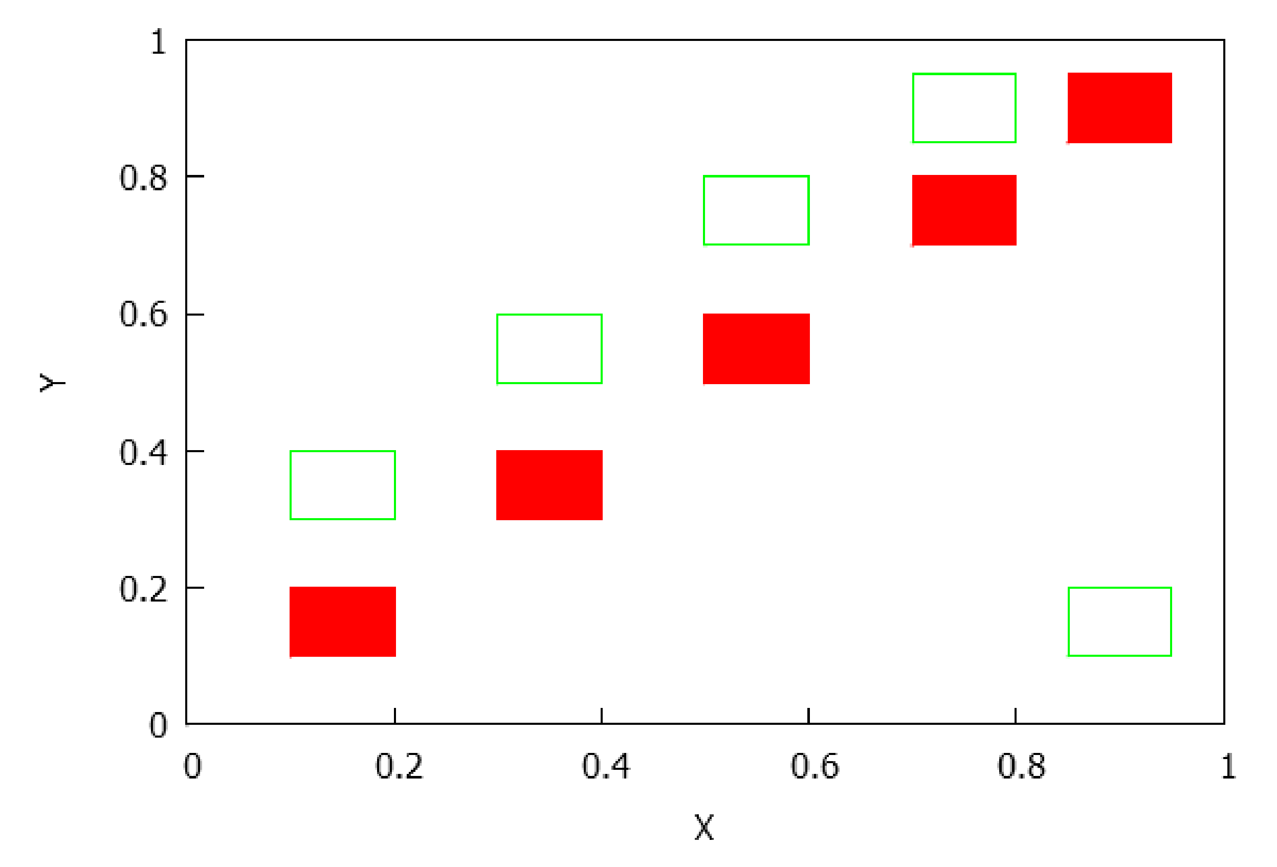
  If $t\ne 1$, there are $k=p=q$ rectangles and there exists an arrangement of the indexes such that $R_i=I_i\times J_i$ for $i=1,\dots ,k$. It is clear that $p_1\left(I_i\right)=p_2\left(J_i\right)=1$ for any $i=1,\dots ,k$. See Figure 5.

  (D2)

  If $t=1$, there are $k=2p=2q$ rectangles and $f_1\left(I_i\right)=J_{i\left(\mathrm{mod}p\right)}$ and $f_2\left(J_i\right)=I_{i+1\left(\mathrm{mod}p\right)}$, where $p\ge 2$. Also, it is held that $p_1\left(I_i\right)=\frac{k}{p}=2$ and $p_2\left(J_i\right)=\frac{k}{p}=2$ for $i=1,\dots p$, see Figure 6.

  Observe that if the number of rectangles k is odd, then only Distribution D1 is possible.
• $f_1\left(A\right)\cap \mathrm{Int}\left(B\right)=\varnothing$. We define

  $$B^{\prime }=\bigcup _{i=1}^p{f}_1\left(I_i\right)=\bigcup _{i=1}^p{J}_i^{\prime }\mathrm{and}{A}^{\prime }=\bigcup _{i=1}^q{f}_2\left(J_i\right)=\bigcup _{i=1}^q{I}_i^{\prime }.$$
  Notice that $B^{\prime }=f_1\left(A\right)$ and $A^{\prime }=f_2\left(B\right)$. Moreover, $B^{\prime }\cap \mathrm{Int}\left(B\right)=\varnothing$ and $A^{\prime }\cap \mathrm{Int}\left(A\right)=\varnothing$. In this case, the number of rectangles, k, is always even, in particular $k=2\ell =2\mathrm{lcm}(p,q)$ as $F^{2r}\left(I_1\times J_1\right)=I_{1+r\left(\mathrm{mod}p\right)}\times J_{1+r\left(\mathrm{mod}q\right)}$ and $F^{2r+1}\left(I_1\times J_1\right)=f_2\left(J_{1+r\left(\mathrm{mod}q\right)}\right)\times f_1\left(I_{1+r\left(\mathrm{mod}p\right)}\right)=I_{1+r\left(\mathrm{mod}q\right)}^{\prime }\times J_{1+r\left(\mathrm{mod}p\right)}^{\prime }$ for $r\in \{1,\dots ,\ell \}.$ The $\omega$-limit set L is given by $L=L_1\cup L_2$, with ${\pi }_1\left(L_1\right)=A$, ${\pi }_2\left(L_1\right)=B$, ${\pi }_1\left(L_2\right)=A^{\prime }$, ${\pi }_2\left(L_2\right)=B^{\prime }$, such that $\mathrm{Int}\left(L_1\right)\cap L_2=\varnothing$. The number of rectangles $R_i$ of $L_1$ is $k_1$ and the number of rectangles $R_i^{\prime }$ of $L_2$ is $k_2$. Observe also that $k_1=k_2=\ell =\mathrm{lcm}(p,q)$, hence $k=2·k_1=2·\ell$ and $R_i=I_{i\left(\mathrm{mod}p\right)}\times J_{i\left(\mathrm{mod}q\right)}$, $R_i^{\prime }=I_{i\left(\mathrm{mod}q\right)}^{\prime }\times J_{i\left(\mathrm{mod}p\right)}^{\prime }$, $i\in \{1,\dots ,\ell \}$, with $p_1\left({\pi }_1\left(R\right)\right)=\frac{\ell }{p}$, $p_2\left({\pi }_2\left(R\right)\right)=\frac{\ell }{q}$ for each R in $L_1$ and $p_1\left({\pi }_1\left(R^{\prime }\right)\right)=\frac{\ell }{q}$, $p_2\left({\pi }_2\left(R^{\prime }\right)\right)=\frac{\ell }{p}$ for each $R^{\prime }$ in $L_2$. Thus, $p_1\left(I_i\right)=p_2\left(J_i^{\prime }\right)=\frac{\ell }{p}=\frac{k}{2p}$ for $i\in \{1,\dots ,p\}$, and $p_2\left(J_i\right)=p_1\left(I_i^{\prime }\right)=\frac{\ell }{q}=\frac{k}{2q}$ for $i\in \{1,\dots ,q\}.$ As we have signaled above, the rectangles of the $\omega$-limit set are described by $R_{i\left(\mathrm{mod}k\right)}=I_{i\left(\mathrm{mod}p\right)}\times J_{i\left(\mathrm{mod}q\right)}$ and $R_{i\left(\mathrm{mod}k\right)}^{\prime }=I_{i\left(\mathrm{mod}q\right)}^{\prime }\times J_{i\left(\mathrm{mod}p\right)}^{\prime }$ for $i=1,\dots ,k$. This case is easily detected when there exists $i\ne j$ such that $p_1\left({\pi }_1\left(R_i\right)\right)=p_2\left({\pi }_2\left(R_j^{\prime }\right)\right)\ne p_1\left({\pi }_1\left(R_j^{\prime }\right)\right)=p_2\left({\pi }_2\left(R_i\right)\right)$. Additionally, if:

  (D3)

  $f_1\left(A\right)\cap B=\varnothing$. There are $2\ell$ connected components, since the number of connected components of $A\cup A^{\prime }$ is $p+q$. See Figure 7.

  (D4)

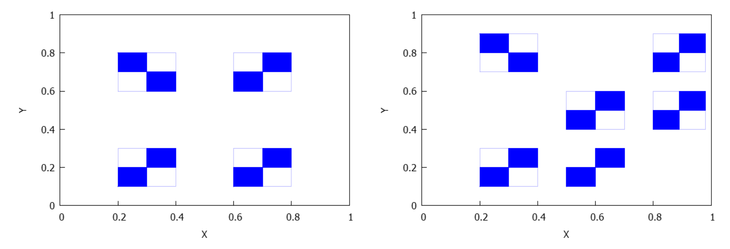
  $f_1\left(A\right)\cap B\ne \varnothing$. The number of connected components depends on the number of connected components of $A\cup A^{\prime }$ and $B\cup B^{\prime }$ which is less than or equal to p and q, respectively, see Lemma 4. Consequently, rectangles can be disjoint, have a common vertex or two common vertices, see Figure 8, Figure 9, Figure 10 and Figure 11. Notice that the case for two common vertices can only be realized by a unique distribution, given precisely by Figure 10; moreover, observe that $R_i\cap R_j^{\prime }\ne \varnothing$ if and only if $I_i\cap I_j^{\prime }\ne \varnothing$ and $J_i\cap J_j^{\prime }\ne \varnothing$.

3.2. A Mixing and B No Mixing

Since B is no mixing and by Definition 2, Lemma 1 and Lemma 2, there are closed intervals $J_i^1$ and $J_i^2$ whose intersection is a fixed point of ${(f_1\circ f_2)}^q$ and such that $J_i=J_i^1\cup J_i^2$, ${(f_1\circ f_2)}^q\left(J_i^1\right)=J_i^2$, ${(f_1\circ f_2)}^q\left(J_i^2\right)=J_i^1$, and ${(f_1\circ f_2)}^{2q}{|}_{J_i^j}$ is mixing on $J_i^j$ for $i=1,2,\dots ,q$ and $j=1,2$. Now, it is not possible that $f_1\left(A\right)\cap \mathrm{Int}\left(B\right)\ne \varnothing$ due to Lemma 3 and the different mixing character of the intervals.

Assume that $L=L_1\cup L_2$ and that the rectangles of $L_1$ and $L_2$ are of type $I_i\times J_j^r$ and type ${\left(I^{\prime }\right)}_j^r\times J_i^{\prime }$ (with $i\in \{1,\dots ,p\},$ $j\in \{1,\dots ,q\},$ $r=1,2$), respectively, where we have implicitly used Proposition 1 as well as the notation

$$f_1\left(A\right)=f_1\left(\bigcup _{i=1}^p{I}_i\right)=\bigcup _{i=1}^p{f}_1\left(I_i\right)=:\bigcup _{i=1}^p{J}_i^{\prime },$$

and

$$f_2\left(B\right)=f_2\left(\bigcup _{i=1}^q\left(J_j^1\cup J_j^2\right)\right)=\bigcup _{j=1}^q\left(f_2\left(J_j^1\right)\cup f_2\left(J_j^2\right)\right)=:\bigcup _{j=1}^q\left({\left(I^{\prime }\right)}_j^1\cup {\left(I^{\prime }\right)}_j^2\right).$$

Next, by assuming that $R_1=I_1\times J_1^1$, we have:

• If $\frac{\ell }{q}$ is odd, $\ell =rq,$ r odd, then ${(f_1\circ f_2)}^{rq}\left(J_j^s\right)=J_j^t$, for all $j=1,\dots ,q$ and $s,t\in \{1,2\}$, $s\ne t$, due to the fact that B is not mixing; then both rectangles $I_i\times J_j^1$ and $I_i\times J_j^2$ belong to $L_1$ (realize that $F^{2\ell }(I_i\times J_j^1)={(f_2\circ f_1)}^{\ell }\left(I_i\right)\times {(f_1\circ f_2)}^{\ell }\left(J_j^1\right)=I_i\times J_j^2$), that is, $I_i\times J_j$ belongs to $L_1$; similarly, both rectangles ${\left(I^{\prime }\right)}_j^1\times J_i$ and ${\left(I^{\prime }\right)}_j^2\times J_i$ belong to $L_2$ and, therefore, the distribution of $L=L_1\cup L_2$ is reduced to the case A and B mixing with $f_1\left(A\right)\cap B=\varnothing$ (distribution D3).
• If $\frac{\ell }{q}$ is even, $\ell =mq,$ m even, now each rectangle of the $\omega$-limit L is the half part of a rectangle $I_i\times J_k$ or $I_j^{\prime }\times J_i^{\prime }$, and the number of rectangles of $L_n$ is equal to ℓ, $n=1,2$, so $\left|L\right|=2\ell$ (notice that, as a consequence of the parity of ℓ, $F^{2\ell }(I_1\times J_1^1)={(f_2\circ f_1)}^{\ell }\left(I_1\right)\times {(f_1\circ f_2)}^{\ell }\left(J_1^1\right)=I_1\times J_1^1$ and consider that $F^t(I_1\times J_1^1)\notin \{I_1\times J_1^1,I_1\times J_2^1\}$ for $0<t<2\ell$).

Thus, we assume that $\frac{\ell }{q}$ is even. The number of rectangles of L must be a multiple of 4. Since $L_1$ has an even number of rectangles, the following cases sum up the possibilities.

(D5)

$f_1\left(A\right)\cap B=\varnothing$. In this case, the $\omega$-limit is a set L which is the union of $L_1$ and $L_2$ both with the same number of rectangles. We also have that $L_i$ has an even number of rectangles for $i=1,2$. Observe that: $p_1\left({\pi }_1\left(R\right)\right)=\frac{\ell }{p}$ and $p_2\left({\pi }_2\left(R\right)\right)=\frac{\ell }{q}$ for each entire rectangle R having the form $I_i\times J_j=I_i\times \left(J_j^1\cup J_j^2\right)$ and each projection of a rectangle of $L_1$ must have a common point with the projection of another rectangle; similarly, $p_2\left({\pi }_2\left(R\right)\right)=\frac{\ell }{p}$ and $p_1\left({\pi }_1\left(R\right)\right)=\frac{\ell }{q}$ for each entire rectangle $R\in L_2$ (having the form ${\left(I^{\prime }\right)}_j\times {\left(J^{\prime }\right)}_i=\left({\left(I^{\prime }\right)}_j^1\cup {\left(I^{\prime }\right)}_j^2\right)\times \left({\left(J^{\prime }\right)}_i\right)$) and each projection of a rectangle must have a common point with the projection of another rectangle. See Figure 12.

(D6)

$f_1\left(A\right)\cap \mathrm{Int}\left(B\right)=\varnothing$ and $f_1\left(A\right)\cap B\ne \varnothing$. By Lemma 4 and Remark 2, we know that each connected component of $A\cup f_2\left(B\right)$ has the form $I_i\cup I_i^{\prime }\cup I_{i+1}$, where $I_i=[a_i,b_i],$ $I_i^{\prime }=[b_i,a_{i+i}],$ $I_{i+1}=[a_{i+1},b_{i+1}],$ for some values $a_i<b_i<a_{i+1}<b_{i+1}$. Notice that $p=2q$, $\ell =p$, $\frac{\ell }{q}=2$; moreover, the number of rectangles in $L=L_1\cup L_2$ is just $4q$. Here, the ‘entire’ rectangles R in $L_1$ have the form $I_i\times J_j=I_i\times \left(J_j^1\cup J_j^2\right)$, and we have $p_1\left({\pi }_1\left(R\right)\right)=\frac{\ell }{p}=1$ and $p_2\left({\pi }_2\left(R\right)\right)=\frac{\ell }{q}=2.$ For rectangles $R^{\prime }$ in $L_2$, having type $\left({\left(I^{\prime }\right)}_i^1\cup {\left(I^{\prime }\right)}_i^2\right)\times J_j^{\prime }$, instead we find $p_1\left({\pi }_1\left(R^{\prime }\right)\right)=\frac{\ell }{q}=2$ and $p_2\left({\pi }_2\left(R\right)\right)=\frac{\ell }{p}=1.$ See Figure 13.

3.3. A and B No Mixing

Realize that if A and B are no mixing, then $f_1\left(A\right)$ and $f_2\left(B\right)$ are also no mixing. We can assume that, except for equivalences, there are closed intervals $I_i^1$ and $I_i^2$, whose intersection is a fixed point of ${(f_2\circ f_1)}^p$ and such that $I_i=I_i^1\cup I_i^2$, ${(f_2\circ f_1)}^p\left(I_i^1\right)=I_i^2$, ${(f_2\circ f_1)}^p\left(I_i^2\right)=I_i^1$ and ${(f_2\circ f_1)}^{2p}{|}_{I_i^j}$ is mixing on $I_i^j$ for $i=1,2,\dots ,p$ and $j=1,2$. A similar situation occurs for B, with $J_j=J_j^1\cup J_j^2$, $j=1,\dots ,q$. We also assume that $R_1=I_1^1\times J_1^1$. Let us assume also that $I_i^1<I_i^2$ and $J_i^1<J_i^2$, where $I<J$ means that $x<y$ for each $x\in I$ and $y\in J$. Now, according to Lemma 4, only the cases $f_1\left(A\right)\cap B=\varnothing$ and $f_1\left(A\right)\cap \mathrm{Int}\left(B\right)\ne \varnothing$ are admissible (notice that the last one is equivalent to $f_1\left(A\right)=B$). Recall that $\ell =\mathrm{lcm}(p,q)$, p and q being the number of intervals in A and B, respectively. Moreover, thanks to the equivalence relation given in Definition 1, we can assume without loss of generality that $(f_2\circ f_1)\left(I_i\right)=I_{i+1\left(\mathrm{mod}p\right)}$ and $(f_1\circ f_2)\left(J_j\right)=J_{j+1\left(\mathrm{mod}q\right)}$.

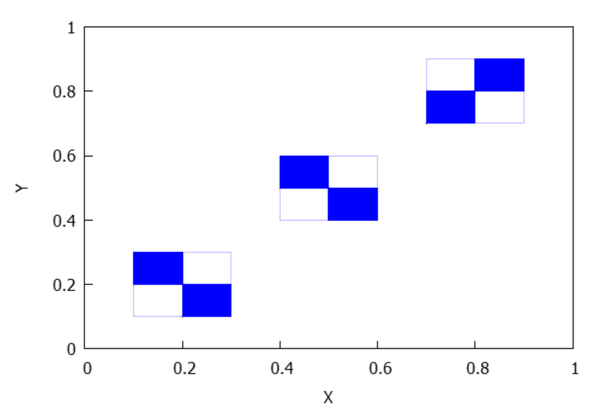
• Case $f_1\left(A\right)\cap B=\varnothing$. Firstly, we claim that the number of rectangles in the orbit of $I_1\times J_1$, ${\mathrm{Orb}}_F(I_1\times J_1)=\{I_1\times J_1,f_2\left(J_1\right)\times f_1\left(I_1\right),(f_2\circ f_1)\left(I_1\right)\times (f_1\circ f_2)\left(J_1\right),\dots \}$, is equal to $2\ell$. To see it, let $\left\{a\right\}=I_1^1\cap I_1^2,$ $\left\{b\right\}=J_1^1\cap J_1^2;$ we know that a (b) is a periodic point of $f_2\circ f_1$ ($f_1\circ f_2$) of period p (q). We assert that $(a,b)$ is a periodic point of F of period $2\ell$. Let m be the order of $(a,b)$ for the map F. Since $F^{2\ell }(a,b)=({(f_2\circ f_1)}^{\ell }\left(a\right),{(f_1\circ f_2)}^{\ell }\left(b\right))=(a,b),$ on the one hand we have $m|2\ell$. Thus, $F^{2m}(a,b)=({(f_2\circ f_1)}^m\left(a\right),{(f_1\circ f_2)}^m\left(b\right))=(a,b)$; on the other hand, we also deduce that $p|m$ and $q|m$, and consequently $\ell |m$. From the above reasoning, either $m=\ell$ or $m=2\ell$. If it were $m=\ell$, with ℓ even, $\ell =2\left(\frac{\ell }{2}\right)$, then $F^{\ell }(a,b)=({(f_2\circ f_1)}^{\frac{\ell }{2}}\left(a\right),{(f_1\circ f_2)}^{\frac{\ell }{2}}\left(b\right))=(a,b)$ and $p|\frac{\ell }{2},q|\frac{\ell }{2}$, in contradiction with the definition of the lowest common multiple. If it were $m=\ell$, with ℓ odd, $\ell =2s+1$, now $F^{2s+1}(a,b)=(a,b)$ would give us ${(f_2\circ f_1)}^s\left(f_2\left(b\right)\right)=a,{(f_1\circ f_2)}^s\left(f_1\left(a\right)\right)=b,$ so $(a,b)\in (A\times B)\cap (f_2\left(B\right)\times f_1\left(A\right))$, that is, $a\in A\cap f_2\left(B\right)$, contrary to our hypothesis. Therefore, $(a,b)$ is F-periodic and its period is $2\ell$. As a consequence, ${\mathrm{Orb}}_F(I_1\times J_1)$ has $2\ell$ different rectangles (maybe with common vertexes). Since $F^{2\ell }(I_1\times J_1)=I_1\times J_1$, and ℓ is the first time s in which ${(f_2\circ f_1)}^s\left(I_1\right)\times {(f_1\circ f_2)}^s\left(J_1\right)=I_1\times J_1,$ we have that ${\mathrm{Orb}}_F(I_1\times J_1)$ has either ℓ or $2\ell$ elements. But the case ℓ is forbidden because then $F^{\ell }(a,b)=(a,b)$ due to the fact that $(a,b),F(a,b),\dots ,$ are the ‘middle points’ of $I_1\times J_1$ and its respective images. This ends the claim.
  The last claim does not imply necessarily that the number k of rectangles in the $\omega$-limit $L={\omega }_F(x,y)={\mathrm{Orb}}_F(I_1^1\times J_1^1)$ must be $2\ell$. It will depend on the parity of $k_1:=\frac{\ell }{p}$ and $k_2:=\frac{\ell }{q}$. Realize that $k_1$ and $k_2$ cannot be even simultaneously, at least some of them are odd.
  If $k_1$ is odd and $k_2$ is even (the case $k_1$ even and $k_2$ odd is analogous), then $F^{2\ell }(I_1^1\times J_1^1)={(f_2\circ f_1)}^{\ell }\left(I_1^1\right)\times {(f_1\circ f_2)}^{\ell }\left(J_1^1\right)=I_1^2\times J_1^1$, and really we have $2\ell$ different rectangles in L because the parts $I_1^1\times J_1^1$ and $I_1^2\times J_1^1$ gives rise to the union of $I_1\times J_1^1$. The distribution that appears is equal to the case mixing–no mixing previously considered, distribution D5.
  If $k_1$ and $k_2$ are both odd integers, then $\ell =p{k}_1=q{k}_2$ and $F^{2\ell }(I_1^1\times J_1^1)={(f_2\circ f_1)}^{\ell }\left(I_1^1\right)\times {(f_1\circ f_2)}^{\ell }\left(J_1^1\right)=I_1^2\times J_1^2$, and in this case we find $4\ell$ different rectangles (notice that $F^{2j}(I_1^1\times J_1^1)\ne I_1^1\times J_1^1$ for $j=1,\dots ,\ell -1$); moreover, the rectangles in the $\omega$-limit L are distributed in two groups of rectangles, namely $L_1$ and $L_2$, with $|L_1|=|L_2|=2\ell$. The distribution of $L_2$ mimics the distribution of $L_1$, shifting the position of the axes. See Figure 14.
  Thus, let us assume $k_1$ and $k_2$ are odd numbers. Then, structures that are made up of two rectangles with a common point appear, which allows us to consider different orientations, namely, $(+)$ and $(-)$ see Figure 15.
  For this case, there must coexist these types of structures with both orientations, but, how many of them?
  In order to describe and count the structures with negative orientation, we proceed as follows. Recall that we assume $A={\cup }_{i=1}^p{I}_i$, $B={\cup }_{j=1}^q{J}_j$, and both ${(f_2\circ f_1)}^p{|}_{I_i}$ and ${(f_1\circ f_2)}^q{|}_{J_j}$ are no mixing. We put $I_i=I_i^1\cup I_i^2,J_j=J_j^1\cup J_j^2,$ with $I_i^1\le I_i^2,J_j^1\le J_j^2.$ Moreover, $p\ge q$, $\ell =\mathrm{lcm}(p,q)$ and $k_1=\frac{\ell }{p}$, $k_2=\frac{\ell }{q}$ are odd integers. If the $\omega$-limit set L is written as $L=L_1\cup L_2$, take into account that we are going to describe the structures with negative orientation in $L_1$, for subrectangles contained in bigger rectangles of type $I_i\times J_j,$ and that we start to iterate with the subrectangle $I_1^1\times J_1^1$.
  For $i=1,\dots ,p$ define $\sigma \left(j\right)\in \{1,2\}$ as the value for which

  $$\begin{array}{cc}\hfill {(f_2\circ f_1)}^i\left(I_1^1\right)& =I_{1+i\left(\mathrm{mod}\right(p\left)\right)}^{\sigma \left(i\right)}.\end{array}$$
  Notice that $\sigma \left(p\right)=2$.
  Similarly, for $j=1,\dots ,q$, define $\tau \left(j\right)\in \{1,2\}$ to be value holding

  $$\begin{array}{cc}\hfill {(f_1\circ f_2)}^j\left(J_1^1\right)& =J_{1+j\left(\mathrm{mod}\right(q\left)\right)}^{\tau \left(j\right)}.\end{array}$$
  From the mixing property of $f_1\circ f_2$, we have $\tau \left(q\right)=2$. In short,

  $$\left(\begin{array}{ccccc}1& 2& \dots & p-1& p\\ \sigma \left(1\right)& \sigma \left(2\right)& \dots & \sigma (p-1)& 2\end{array}\right),\left(\begin{array}{ccccc}1& 2& \dots & q-1& q\\ \tau \left(1\right)& \tau \left(2\right)& \dots & \tau (q-1)& 2\end{array}\right).$$
  We can extend the definition to two sequences

  $$\begin{array}{c}\hfill \sigma :\mathbb{N}\to {\{1,2\}}^{\mathbb{N}},\\ \hfill \tau :\mathbb{N}\to {\{1,2\}}^{\mathbb{N}},\end{array}$$

  in this manner: from the mixing properties of $f_2\circ f_1$ and $f_1\circ f_2$, we know, for instance, that ${(f_2\circ f_1)}^{p+1}\left(I_1^1\right)=(f_2\circ f_1)\left(I_1^2\right)=I_1^{\overline{\sigma \left(1\right)}},$ where we use the notation $\overline{r}$ to denote the value

  $$\overline{r}=1+r\left(\mathrm{mod}\left(2\right)\right)\in \{1,2\};$$

  therefore, we can define $\sigma (p+j)=\overline{\sigma \left(j\right)}$ for $j=1,\dots ,p$. Similarly, ${(f_2\circ f_1)}^{2p+1}\left(I_1^1\right)=(f_2\circ f_1)\left(I_1^1\right)=I_1^{\sigma \left(1\right)},$ and we can define $\sigma (2p+j)=\sigma \left(j\right)$ for $j=1,\dots ,p$. Thus,

  $$\sigma \left(n\right)=\left\{\begin{array}{cc}\sigma \left(r\right),& \mathrm{if}n=\left(2j\right)p+r,\mathrm{for}\mathrm{some}j\ge 0,r\in \{1,\dots ,p\},\\ \overline{\sigma \left(r\right)},& \mathrm{if}n=(2j+1)p+r,\mathrm{for}\mathrm{some}j\ge 0,r\in \{1,\dots ,p\}.\end{array}\right.$$
  Notice that ${(f_2\circ f_1)}^n\left(I_1^1\right)=I_{1+n\left(\mathrm{mod}\right(p\left)\right)}^{\sigma \left(n\right)}$. Similarly, we extend $\tau$ as

  $$\tau \left(n\right)=\left\{\begin{array}{cc}\sigma \left(s\right),& \mathrm{if}n=\left(2j\right)q+s,\mathrm{for}\mathrm{some}j\ge 0,s\in \{1,\dots ,q\},\\ \overline{\sigma \left(s\right)},& \mathrm{if}n=(2j+1)q+s,\mathrm{for}\mathrm{some}j\ge 0,s\in \{1,\dots ,q\}.\end{array}\right.$$
  Here, ${(f_1\circ f_2)}^n\left(I_1^1\right)=I_{1+n\left(\mathrm{mod}\right(q\left)\right)}^{\tau \left(n\right)}$.
  Notice that $F^{2\ell }(I_1^1\times J_1^1)={(f_2\circ f_1)}^{\ell }\left(I_1^1\right)\times {(f_1\circ f_2)}^{\ell }\left(J_1^1\right)=I_1^{\sigma \left(\ell \right)}\times J_1^{\tau \left(\ell \right)},$ and the same time $F^{2\ell }(I_1^1\times J_1^1)={\left({(f_2\circ f_1)}^p\right)}^{k_1}\left(I_1^1\right)\times {\left({(f_1\circ f_2)}^q\right)}^{k_2}\left(J_1^1\right)=I_1^2\times J_1^2.$ This implies that $\sigma \left(\ell \right)=\tau \left(\ell \right)=2$ because $k_1$ and $k_2$ are odd integers, and we can observe that from this point the values of the orbit of $I_1^1\times J_1^1$ belong to the same structure.
  Notice also that if $i\in \{1,\dots ,\ell \}$ then

  $$F^{2(\ell +i)}(I_1^1\times J_1^1)=F^{2i}(I_1^2\times J_1^2)=I_{1+i\left(\mathrm{mod}\right(p\left)\right)}^{\overline{\sigma \left(i\right)}}\times J_{1+i\left(\mathrm{mod}\right(q\left)\right)}^{\overline{\tau \left(i\right)}},$$

  (5)

  whenever $F^{2i}(I_1^1\times J_1^1)=I_{1+i\left(\mathrm{mod}\right(p\left)\right)}^{\sigma \left(i\right)}\times J_{1+i\left(\mathrm{mod}\right(q\left)\right)}^{\tau \left(i\right)}.$ As we see, this again guarantees that our extensions, $\sigma ,\tau :\mathbb{N}\to {\{1,2\}}^{\mathbb{N}}$ are well defined.
  Additionally, in order to check if the structure has positive or negative orientation, it suffices, according to (5), to analyze the pairs $\left(\sigma \right(i),\tau (i\left)\right)$, with $i\in \{1,\dots ,\ell \}$. To this regard, define

  $$\mathrm{O}\left(i\right)=\left(\sigma \right(i),\tau (i\left)\right),i=1,\dots ,\ell .$$
  If $\mathrm{O}\left(i\right)=(r,r)$ for some $r\in \{1,2\}$, we say that $I_{1+i\left(\mathrm{mod}\right(p\left)\right)}^{\sigma \left(i\right)}\times J_{1+i\left(\mathrm{mod}\right(q\left)\right)}^{\tau \left(i\right)}$ has positive orientation; if, on the contrary, $\mathrm{O}\left(i\right)=(r,\overline{r})$, for $r\in \{1,2\}$, we say that the structure has negative orientation.
  Consequently, if we try to count the positive and negative orientations, we only need to see the character of the pairs $\mathrm{O}\left(i\right)=\left(\sigma \right(i),\tau (i\left)\right),i=1,\dots ,\ell .$
  For instance, if $p=5$ and $q=3$, with

  $$\left(\begin{array}{ccccc}1& 2& 3& 4& 5\\ 1& 2& 2& 1& 2\end{array}\right),\left(\begin{array}{ccc}1& 2& 3\\ 2& 1& 2\end{array}\right),$$

  we obtain:

  $$\begin{array}{cccccc}(1,1)& \to & \left(\sigma \right(1),\tau (1\left)\right)=(1,2)& \to & \left(\sigma \right(2),\tau (2\left)\right)=(2,1)& \to \\ \left(\sigma \right(3),\tau (3\left)\right)=(2,2)& \to & (\sigma \left(4\right),\overline{\tau \left(1\right)})=(1,1)& \to & (\sigma \left(5\right),\overline{\tau \left(2\right)})=(2,2)& \to \\ (\overline{\sigma \left(1\right)},\overline{\tau \left(3\right)})=(2,1)& \to & (\overline{\sigma \left(2\right)},\tau \left(1\right))=(1,2)& \to & (\overline{\sigma \left(3\right)},\tau \left(2\right))=(1,1)& \to \\ (\overline{\sigma \left(4\right)},\tau \left(3\right))=(2,2)& \to & (\overline{\sigma \left(5\right)},\overline{\tau \left(1\right)})=(1,1)& \to & (\sigma \left(1\right),\overline{\tau \left(2\right)})=(1,1)& \to \\ (\sigma \left(2\right),\overline{\tau \left(3\right)})=(2,1)& \to & \left(\sigma \right(3),\tau (1\left)\right)=(2,2)& \to & \left(\sigma \right(4),\tau (2\left)\right)=(1,1)& \to \\ \left(\sigma \right(5),\tau (3\left)\right)=(2,2)& \to & (\overline{\sigma \left(1\right)},\overline{\tau \left(1\right)})=(2,2),& \hspace{1em}& \hspace{1em}& \hspace{1em}\end{array}$$

  and from this point we will obtain the opposite orbit to the last $\ell =15$ iterates. In this case, the number of negative orientations is 5.
  Once we have described how to count the orientations in $L_1$, for the set $L_2$ that has subrectangles of type ${\left(I^{\prime }\right)}_{i\left(\mathrm{mod}\right(q\left)\right)}^s\times {\left(J^{\prime }\right)}_{i\left(\mathrm{mod}\right(p\left)\right)}^t$, with $s,t\in \{1,2\}$, we proceed in a similar way to that described for $L_1$. Since we have assumed that $f_1\left(I_i\right)=J_i^{\prime }$ and $f_2\left(J_i\right)=I_i^{\prime }$, we write $f_2\left(J_1^1\right)\times f_1\left(I_1^1\right)={\left(I^{\prime }\right)}_1^{\mu \left(0\right)}\times {\left(J^{\prime }\right)}_1^{\rho \left(0\right)}$, for suitable $\mu \left(0\right),\rho \left(0\right)\in \{1,2\}$. Now, we have to define $\mu \left(s\right)$, $s=1,\dots ,q$ as the value in $\{1,2\}$ for which ${(f_2\circ f_1)}^s\left({\left(I^{\prime }\right)}_1^{\mu \left(0\right)}\right)={\left(I^{\prime }\right)}_{1+s\left(\mathrm{mod}\right(q\left)\right)}^{\mu \left(s\right)}$, and, similarly, $\rho \left(t\right)\in \{1,2\}$ will be characterized by ${(f_1\circ f_2)}^t\left({\left(J^{\prime }\right)}_1^{\rho \left(0\right)}\right)={\left(J^{\prime }\right)}_{1+t\left(\mathrm{mod}\right(p\left)\right)}^{\rho \left(t\right)}$, for $t=1,\dots ,p.$ Notice that $\mu \left(q\right)=\overline{\mu \left(0\right)}$ and $\rho \left(p\right)=\overline{\rho \left(0\right)}$. By extending $\mu$ and $\rho$ to all positive integers, for counting the negative orientations we will have to pick the pairs $\left(\mu \right(i),\rho (i\left)\right)$ with $\mu \left(i\right)\ne \rho \left(i\right)$, for $i=1,\dots ,\ell$.
• Case $f_1\left(A\right)\cap \mathrm{Int}\left(B\right)\ne \varnothing$. This means that $p=q=\ell$, in fact $f_1\left(A\right)=B$ and $f_2\left(B\right)=A$. Firstly, let us show that the point $(a,b)\in I_1\times J_1$, given by $a=I_1^1\cap I_1^2,b=J_1^1\cap J_1^2,$ is F-periodic and its (minimal) period m can be ℓ or $2\ell$. Indeed, it is clear that $F^{2\ell }(a,b)=({(f_2\circ f_1)}^{\ell }\left(a\right),{(f_1\circ f_2)}^{\ell }\left(b\right))=(a,b)$ because a and b are fixed points of ${(f_2\circ f_1)}^{\ell }$ and ${(f_1\circ f_2)}^{\ell }$, respectively, as a consequence of the no mixing property satisfied by A and B, and the fact that $\ell =p=q$. On the other hand, if $n<\ell$ were the order of $(a,b)$, then $(a,b)=F^{2n}(a,b)=({(f_2\circ f_1)}^n\left(a\right),{(f_1\circ f_2)}^n\left(b\right))$ would imply that $\ell |n$, a contradiction. Therefore, m is either ℓ or $2\ell$.
  Consequently, we must distinguish two cases according to whether the order m of the aforementioned F-periodic $(a,b)$ is ℓ or $2\ell$:

  (i.O)

  If $m=\ell$, we affirm that the number k of rectangles in $L={\omega }_F(x,y)$ is $k=\ell$, and in fact ${\omega }_F(x,y)$ is composed of ℓ rectangles of type $I_i\times J_j$. To prove it, recall that we are assuming that $(x,y)\in R_1=I_1^1\times J_1^1\subset I_1\times J_1$. Notice that $F^{\ell }(a,b)=(a,b)\in I_1\times J_1$, so $F^{\ell }(I_1^1\times J_1^1)=I_1^i\times J_1^j$ for some $i,j\in \{1,2\}$. If $i=j=1$, then we would have $F^{2\ell }(I_1^1\times J_1^1)=F^{\ell }(I_1^1\times J_1^1)=I_1^1\times J_1^1$, but at the same time, for the decomposition of A and B obtained for their no mixing property, $F^{2\ell }(I_1^1\times J_1^1)={(f_2\circ f_1)}^{\ell }\left(I_1^1\right)\times {(f_1\circ f_2)}^{\ell }\left(J_1^1\right)=I_1^2\times J_1^2$, it is impossible. If $i=j=2$, now $F^{\ell }(I_1^1\times J_1^1)=I_1^2\times J_1^2$ and since also $F^{2\ell }(I_1^1\times J_1^1)=I_1^2\times J_1^2$, we would obtain $F^{s\ell }(I_1^2\times J_1^2)=I_1^2\times J_1^2$ for all $s\ge 1$, a new contradiction (at least, $F^{2\ell }(I_1^2\times J_1^2)=I_1^1\times J_1^1$). Therefore, $i\ne j$, which implies that either $F^{\ell }(I_1^1\times J_1^1)=I_1^1\times J_1^2$ or $F^{\ell }(I_1^1\times J_1^1)=I_1^2\times J_1^1$. For instance, if $F^{\ell }(I_1^1\times J_1^1)=I_1^1\times J_1^2$, then $F^{3\ell }(I_1^1\times J_1^1)=F^{2\ell }(I_1^1\times J_1^2)=I_1^2\times J_1^1$, and thus all the rectangle $I_1\times J_1$ is included in ${\mathrm{Orb}}_F(I_1^1\times J_1^1)$. From here, and taking into account that an entire rectangle only contains at most a unique point of $\mathrm{Orb}F(a,b)$, we deduce that $\left|L\right|=\ell$, and ${\omega }_F(x,y)$ is composed of $k=\ell$ rectangles of type $I_i\times J_j$. Even more, its distribution follows the pattern of Distribution D1, and with equivalence we can reorder the intervals in such a way that $f_1\left(I_i\right)=J_{i+1\left(\mathrm{mod}p\right)}$ and $f_2\left(J_i\right)=I_{i+1\left(\mathrm{mod}p\right)}$ for $i=1,\dots ,p$. See Figure 16.

  Finally, notice that only the case ℓ odd is permitted here, since if ℓ is even, we would have $(a,b)=F^{\ell }(a,b)$ and then ${\left(f_2\circ f_1\right)}^{\frac{\ell }{2}}\left(a\right)=a$, ${\left(f_1\circ f_2\right)}^{\frac{\ell }{2}}\left(b\right)=b$, impossible (realize that a and b are ℓ-periodic points of $f_2\circ f_1$ and $f_1\circ f_2$, respectively).

  (ii.E)

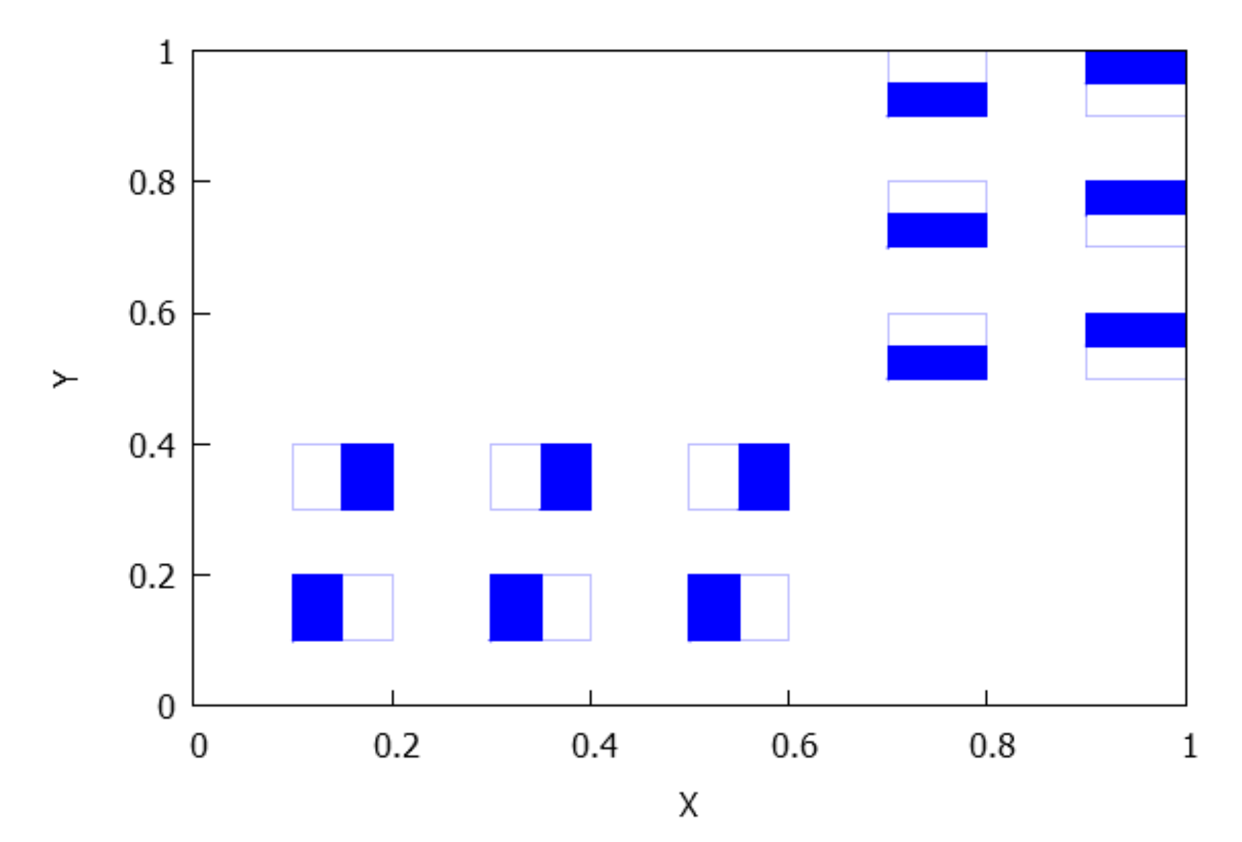
  If $m=2\ell$, we assert that $\left|L\right|=4\ell$ and, to be more precise, $L={\omega }_F(x,y)$ is composed of $4\ell$ rectangles having type $I_i^u,J_j^v$ for some $i,j\in \{1,\dots ,2\ell \},$ $u,v\in \{1,2\}$, such that each of them are included in $I_i\times J_j$, with a common vertex given by a point of the orbit of $(a,b)$. To prove it, first notice that ${\mathrm{Orb}}_F(a,b)=:\{(x_i,y_i):i=1,\dots ,2\ell \}\subseteq {\mathrm{Orb}}_{(f_2\circ f_1)}\left(a\right)\times {\mathrm{Orb}}_{(f_1\circ f_2)}\left(b\right)$, so from Lemma 5 and Theorem 3-(2) we deduce that for any $i\in \{1,\dots ,2\ell \}$ there exist $r,s\in \{1,\dots ,2\ell \}$, $r\ne s$, such that $x_i=x_r$, $y_i=y_s$. This implies that the F-orbit of $(a,b)$ is included in $2\ell$ entire rectangles of type $I_r\times J_s.$ On the other hand, $F^{2\ell }(I_1^1\times J_1^1)={(f_2\circ f_1)}^{\ell }\left(I_1^1\right)\times {(f_1\circ f_2)}^{\ell }\left(J_1^1\right)=I_1^2\times J_1^2$, and $F^j(I_1\times J_1)\cap \left(I_1\times J_1\right)=\varnothing$ for $j=1,\dots ,\ell$ because $F^j(a,b)\ne (a,b)$ for $j\in \{1,\dots ,\ell \}$ and, according to the distribution provided for Theorem 3 to the orbit of $(a,b)$, each entire rectangle $I_i\times J_j$ only contains at most a unique point of ${\mathrm{Orb}}_F(a,b).$ All the above details allow us to conclude that $k=\left|L\right|=4\ell$ and each rectangle $I_i\times J_j$ containing a point of ${\mathrm{Orb}}_F(a,b)$ is divided into two different subintervals with disjoint interiors and a point in ${\mathrm{Orb}}_F(a,b)$ as common vertex, see Figure 17, and therefore we obtain a structure of the type described in Figure 15.

  Observe that if the position of the intervals is shifted, for example if $I_i^1>I_i^2$, for any i, then the orientation of every structure in the column i changes. This case is the same as that obtained in Distribution D2, but changing the entire rectangle by two subrectangles of the type given in Figure 15.

3.4. The Converse Result for the Non-Empty Interior Case

Until now, we have described the structure of $\omega$-limit sets of Cournot maps with non-empty interior. Of course, given one of these structures L, up to equivalences, it is natural to ask whether it is possible or not to find a Cournot map F and a point $(x,y)\in I^2$ such that ${\omega }_F(x,y)=L$. The answer is the affirmative. The general strategy for this construction relies on the fact that we can take advantage of our knowledge of interval maps $f:I\to I$ exhibiting union of intervals ${\bigcup }_{i=1}^m{I}_i$ as $\omega$-limit sets for suitable points $x\in I$. For instance, for any interval $J=[a,b],$ there is a continuous map $f:J\to J$ with $f\left(a\right)=a$ and $f\left(b\right)=b$ such that f is topologically mixing (see ([1], [p. 162])).

In order to illustrate it, we do the corresponding converse result for Distributions D1 (with k odd), with the hope that the other cases can be managed for the reader without any difficulty.

(D1) Assume that $L={\bigcup }_{i=1}^k(I_i\times J_i)$, k odd, and $I_i,J_i$ verify $\left(D1\right),$ that is:

$L={\bigcup }_{i=1}^k{R}_i={\bigcup }_{i=1}^k(I_{{\alpha }_i}\times J_{{\beta }_i}),$ with $I_{{\alpha }_i}\ne I_{{\alpha }_j},$ $J_{{\beta }_i}\ne J_{{\beta }_j},$ if $i\ne j,$

${\pi }_1\left(L\right)={\bigcup }_{i=1}^k{I}_{{\alpha }_i}=A,$${\pi }_2\left(L\right)={\bigcup }_{i=1}^k{J}_{{\beta }_i}=B.$

To simplify the notation, let ${\alpha }_i=i$ and ${\beta }_j=j$, that is,

$$\begin{array}{cc}\hfill A:=& {\bigcup }_{i=1}^k{\pi }_1\left(R_i\right)={\bigcup }_{i=1}^k{I}_i,\\ \hfill B:=& {\bigcup }_{i=1}^k{\pi }_2\left(R_i\right)={\bigcup }_{i=1}^k{J}_i.\end{array}$$

Write $I_i=\left[a_{i\left(1\right)},a_{i\left(2\right)}\right],J_i=\left[b_{i\left(1\right)},b_{i\left(2\right)}\right].$ We then define $f_1\in C(I,I)$ in such a way that

$$f_1\left(\{a_{i\left(1\right)},a_{i\left(2\right)}\}\right)=b_{i+1\left(1\right)},f_i\left(\frac{a_{i\left(1\right)}+a_{i\left(2\right)}}{2}\right)=b_{i+1\left(2\right)},$$

and linear in the rest of $I_i$, $i=1,\dots ,k$. Also, we define a map $f_2\in C(I,I)$ holding $f_2\left(J_i\right)=I_{i+1}$ in a linear way (change of variables) for $i=1,\dots ,k$. Then, it is straightforward to see that ${\mathrm{Orb}}_F(I_1\times J_1)=L.$ Moreover, $\left(f_2\circ f_1\right)\left(I_i\right)=I_{i+2\mathrm{mod}\left(k\right)},$ $\left(f_1\circ f_2\right)\left(J_i\right)=J_{i+2\mathrm{mod}\left(k\right)},$ $i\in \{1,\dots ,k\}.$ Since k is odd, from the definitions of $f_j$ we deduce that $f_2\circ f_1$ is mixing on A, $f_1\circ f_2$ is mixing on B, and $f_1\left(A\right)=B$, $f_2\left(B\right)=A.$ According to Theorem 2, there exists $(x,y)\in I^2$ such that ${\omega }_{F^{2k}}(x,y)=I_1.$ Then ${\omega }_F(x,y)=\mathrm{Orb}(I_1\times J_1)=L.$

4. Applications to Economic Models

In the seminal paper of Day [19] it was highlighted that complex behavior that can be described as chaotic can emerge from simple economic structures. This fact has had as a consequence for the increasing interest in economic dynamics, which is supported by the large amount of related literature published since then.

In this frame, oligopoly structure plays an important role. The assumption that only a few firms can compete makes sense in some markets in which the goods are perfectly substitutable [20]. In the decision process, each firm adjusts its output (product decision) based on the expectation over the other firm’s output decisions. Under this premise, firms take their decisions simultaneously. In an oligopoly the supply side is (not perfectly) competitive—as we often say “Cournot competition”. A duopoly is an oligopoly in which the number of firms is equal to two. Following Friedman [21], “a duopoly is a market in which two firms sell a product to a large number of consumers. Each consumer is too small to affect the market price for the product, that is, on the buyers’ side, the market is competitive.”

Different theoretical models of duopoly have been considered [21]. In 1838, Cournot [22] proposed a non-collusive duopoly model. In this duopoly model, firms decide their output levels simultaneously, that is, firms compete in quantities and it is assumed that price is given by the market. Moreover, each firm seeks to maximize the profit taking into account the decision of the competitor. Cournot duopoly was considered in [17], where the complexity of the dynamics was established. Later, Dana and Montrucchio [13] gave more details about the dynamical properties of the Cournot model. More recently, Pražák and Kovárník have considered in [15] a nonlinear inverse demand function and have shown bifurcation diagrams of the duopoly model.

Antitriangular maps are closely related to Cournot duopoly models. In this section we deal with the type of $\omega$-limits of several Cournot duopoly models in which dynamics is led by antitriangular maps.

Let us notice the relevance of this topic by highlighting its possible interest in implications for strategic decisions. In this direction, cyclical phenomena have an important role in economics in the analysis of the dynamics and fluctuations of the economic activity in a model. A cycle of length n is the orbit of a periodic point. In the matter at hand, that is, $\omega$-limits of non-empty interior of Cournot maps, the full description of the structure is useful in the sense that it provides information about chaotic orbits (realize that $\omega$-limits with non-empty interior appear when the Cournot map F is chaotic). A cyclical movement appears if, in the definition of cycle, we replace points by rectangles, since in each step the point of the chaotic orbit belongs to the corresponding rectangle and this turns on the fact that in each step we have boundaries (restrictions) for the values of the outputs because the boundaries of the rectangles limit the output values of the production firms when initial conditions have been fixed. In this way, the restriction of the regions of $\omega$-limits in Cournot duopolies plays an important role in the analysis of dynamics. Therefore, the distribution of the $\omega$-limits gives us information about the possible layouts in the rectangles giving the feasible region in which both firms take their output values, the rectangles being covered following a “cyclical process”.

4.1. Puu’s Duopoly

The following duopoly model was proposed by Puu [23]. In this model, the goods produced for both firms are equivalent and the demand function is isoelastic. It is assumed that the price is given by

$$p=\frac{1}{x+y},$$

where x and y are the outputs of firms X and Y respectively. The costs are assumed to be linear with the form $c_1\left(x\right)=c_{1}x$ and $c_2\left(y\right)=c_{2}y$, where $c_1$ and $c_2$, the marginal costs, will be the model parameters. Obviously, now profits are given by

$${\Pi }_1=\frac{x}{x+y}-c_{1}x,$$

$${\Pi }_2=\frac{y}{x+y}-c_{2}y.$$

Considering that the objective of the firms is to maximize their own profits, the equations $\frac{\partial {\Pi }_1}{\partial x}=0$ and $\frac{\partial {\Pi }_2}{\partial y}=0$ give us

$$x=\sqrt{\frac{y}{c_1}}-y,$$

$$y=\sqrt{\frac{x}{c_2}}-x.$$

Finally, the reaction map is

$$F(x,y)=(f_2\left(y\right),f_1\left(x\right))=\left(max\{\sqrt{\frac{y}{c_1}}-y,0\},max\{\sqrt{\frac{x}{c_2}}-x,0\}\right),$$

which is an antitriangular map in which has been introduced the max function due to the fact that productions cannot be negative. It is assumed without loss of generality that $c_1\ge c_2$, and we can compute $\omega$-limit sets, see some examples in Figure 18 (we have used the software Mathematica for generating Figure 18, Figure 19, Figure 20, Figure 21, Figure 22 and Figure 23). More details about the dynamics of the model can be found in [24].

4.2. Kopel’s Duopoly

M. Kopel introduced in [14] a general Cournot duopoly model in which two firms, X and Y, plan their productions, $x_t$, $y_t$, at time t, following the system of difference equations:

$$\begin{array}{cc}\hfill x_{t+1}& =max\{0,(1-{\lambda }_1)x_t+{\lambda }_1{\mu }_1{y}_t(1-y_t)\},\hfill \\ \hfill y_{t+1}& =max\{0,(1-{\lambda }_2)y_t+{\lambda }_2{\mu }_2{x}_t(1-x_t)\},\hfill \end{array}$$

(6)

where ${\lambda }_i\in [0,1]$ and ${\mu }_i>0$ for $i=1,2$. The positive parameters ${\mu }_i$ measure the intensity of the effect that one firm’s action has on the other firm, see also [25] for more details. Then, the two-dimensional map

$$R_{{\lambda }_1,{\lambda }_2,{\mu }_1,{\mu }_2}(x,y):=(max\{0,(1-{\lambda }_1)x+{\lambda }_1{\mu }_{1}y(1-y)\},max\{0,(1-{\lambda }_2)y+{\lambda }_2{\mu }_{2}x(1-x)\}),$$

describes the simultaneous choices of both firms.

Observe that taking ${\lambda }_1={\lambda }_2=1$, a Cournot duopoly model is obtained, given as

$$F(x,y)=(max\{0,{\mu }_{1}y(1-y)\},max\{0,{\mu }_{2}x(1-x)\}).$$

(7)

In Figure 19, we have shown some $\omega$-limits for the map (7). We have selected some of them. To get it, we have used random initial conditions, with 6 decimal digits by default.

4.3. Matsumoto-Nonaka’s Model

In [26] a two–market model consisting of two firms that produce differentiated goods is introduced, see also [27]. The first firm produces good x in the first market and the second one produces good y in the second market. In this model, different externalities affect the dynamics.

As in the previous subsection, in [26] a more general model is introduced. Nevertheless, we are interested in the particular case in which inverse demand functions are given by

$$\begin{array}{cc}\hfill p_1(x,y)& ={(\alpha -1)}^2-\frac{x}{2}+{\left(\alpha y\right)}^2,\hfill \\ \hfill p_2(x,y)& =1-\frac{y}{2}+{\left(\beta x\right)}^2,\hfill \end{array}$$

where $p_1$ and $p_2$ are the market prices of goods x and y, respectively, and $\alpha \in [1,2]\subset \mathbb{R}$ and $\beta \in [0,2]\subset \mathbb{R}$. Each firm decides future production depending on the other firm’s choice and production externalities. Cost functions are given by

$$\begin{array}{cc}\hfill C_1(x,y)& =2(\alpha -1)\alpha xy,\hfill \\ \hfill C_2(x,y)& =2\beta xy,\hfill \end{array}$$

and the profit function of each firm is given by

$$\begin{array}{cc}\hfill {\Pi }_1(x,y)& =p_1(x,y)x-C_1(x,y)=\left({(\alpha -1)}^2-\frac{x}{2}+{\alpha }^2{y}^2\right)x-2(\alpha -1)\alpha xy,\hfill \\ \hfill {\Pi }_2(x,y)& =p_2(x,y)y-C_2(x,y)=\left(1-\frac{y}{2}+{\beta }^2{x}^2\right)y-2\beta xy.\hfill \end{array}$$

(8)

As assumed above, each firm tends to maximize its profit. In order to do this the firms can choose their production levels, which would affect to the other firm. The first firm maximizes the profit with respect to x and the same occurs for the second firm with respect to y. The reaction functions of the firms are given by

$$\begin{array}{cc}\hfill f_{\alpha }\left(y\right)& ={(\alpha y-\alpha +1)}^2,\hfill \\ \hfill g_{\beta }\left(x\right)& ={(\beta x-1)}^2.\hfill \end{array}$$

Now, the function

$$R_{\alpha ,\beta }(x,y)=(f_{\alpha }\left(y\right),g_{\beta }\left(x\right))=({(\alpha y-\alpha +1)}^2,{(\beta x-1)}^2),$$

is the reaction function for the outcome $(x,y)$. The iterations are given by

$$\begin{array}{cc}\hfill x_{t+1}& =f_{\alpha }\left(y_t\right)={(\alpha y_t-\alpha +1)}^2,\hfill \\ \hfill y_{t+1}& =g_{\beta }\left(x_t\right)={(\beta x_t-1)}^2,\hfill \end{array}$$

that is,

$$(x_{t+1},y_{t+1})=F_{\alpha ,\beta }(x_t,y_t)=(f_{\alpha }\left(y_t\right),g_{\beta }\left(x_t\right)),$$

where $\alpha \in [1,2]\subset \mathbb{R}$ and $\beta \in [0,2]\subset \mathbb{R}$. Thus, the reaction map $F_{\alpha ,\beta }$ is a Cournot map from $[0,1]\times [0,1]$ into $[0,1]\times [0,1]$. In this situation, we obtain some $\omega$-limits, the results are shown in Figure 20.

4.4. Cournot Duopoly When the Competitors Operate under Capacity Constraints

In [28] A. Norin and T. Puu introduced a Cournot duopoly where the competitors have capacity constraints. The production cost of the firms are given by

$$\begin{array}{cc}\hfill T{C}_1\left(x\right)& =-log\left(1-\frac{x}{u}\right),\hfill \\ \hfill T{C}_2\left(y\right)& =-log\left(1-\frac{y}{v}\right),\hfill \end{array}$$

(9)

where u and v denote the capacity limits and x and y denote the supplies of the two competitors. Observe that when $x=y=0$ then the total costs are zero and tend to infinity when production approaches capacity limits. The price p is given by $p=\frac{1}{x+y}$ and the profits are

$$\begin{array}{cc}\hfill {\prod }_X(x,y)& =p·x-T{C}_1\left(x\right)=\frac{x}{x+y}+log\left(1-\frac{x}{u}\right),\hfill \\ \hfill {\prod }_Y(x,y)& =p·y-T{C}_2\left(y\right)=\frac{y}{x+y}+log\left(1-\frac{y}{u}\right).\hfill \end{array}$$

(10)

To maximize the profits (10) we get the following equations

$$\begin{array}{cc}\hfill \frac{\partial {\prod }_X}{\partial x}(x,y)& =\frac{y}{{(x+y)}^2}-\frac{1}{u-x}=0,\hfill \\ \hfill \frac{\partial {\prod }_Y}{\partial y}(x,y)& =\frac{x}{{(x+y)}^2}-\frac{1}{v-y}=0.\hfill \end{array}$$

(11)

From the previous system of Equation (11), solving the first for x and the second for y (see [28] for details), the following reaction functions are obtained

$$\begin{array}{cc}\hfill f_u\left(y\right)& =max\left\{0,\frac{1}{2}\sqrt{4uy+5y^2}-\frac{3}{2}y\right\}\hfill \\ \hfill f_v\left(x\right)& =max\left\{0,\frac{1}{2}\sqrt{4vx+5x^2}-\frac{3}{2}x\right\},\hfill \end{array}$$

(12)

since clearly productions cannot be negative. Hence, the reaction map we construct is a Cournot map

$$F_{u,v}(x,y)=(f_u\left(y\right),f_v\left(x\right)).$$

Different $\omega$-limits for the model are shown in Figure 21, where the initial conditions are $x_0=0.2$ and $y_0=0.3$. We have computed orbits of length equal to 200,000 and we have drawn the last 100,000 points.

4.5. A Recurrent Class of Two-Dimensional Endomorphisms

The class of maps given by $F(x,y)=(y,h(x\left)\right)$, where $h\left(x\right)$ is a continuous function, piecewise continuously differentiable, has been considered among others in [29], and in this framework this kind of map provides us another different example to which we can apply this analysis.

Observe that $F^2(x,y)=(h\left(x\right),h\left(y\right))$. Following [29] we consider the map $h\left(x\right)=-\alpha x+\beta g\left(\gamma x\right)$, where

$$g\left(x\right)=\left\{\begin{array}{cc}4\mu x(1-x)\hfill & \mathrm{if}0<x<1(\mu >0),\hfill \\ 0\hfill & \mathrm{otherwise}.\hfill \end{array}\right.$$

The parameters satisfy $0<\alpha <1$, $-1<\beta <0$ and $\gamma <0$. In our particular case, the parameters will use in the simulations are fixed, namely $\alpha =0.62386015$, $\beta =-0.790837347$ and $\gamma =-0.85446789$. See results in Figure 22 and Figure 23.

5. Some Advances in the Empty-Interior Case

For a Cournot map, we already know the topological structure of an $\omega$-limit set with empty interior, see Theorem 1. Essentially, the situation is similar to the interval case, the $\omega$-limit set is a nowhere dense set. In the interval case this means that the set is totally disconnected. This changes for Cournot maps, we can find $\omega$-limit sets with empty interior and locally connected, even connected.

Our first example shows an $\omega$-limit set of empty interior homeomorphic to the circle ${\mathbb{S}}^1=\left\{z\in \mathbb{C}:\left|z\right|=1\right\}.$ Consider a transitive map $f_1:[0,1]\to [0,1]$ with $f_1\left(0\right)=1$ and $f_1\left(1\right)=0$; for instance, take

$$f_1\left(x\right)=\left\{\begin{array}{c}1-2x,\mathrm{if}x\in [0,\frac{1}{2}],\\ T\left(2(x-\frac{1}{2})\right),\mathrm{if}x\in [\frac{1}{2},1],\end{array}\right.$$

where T is the well-known tent map $T\left(x\right)=1-|1-2x|,x\in [0,1].$

$f_1$ being (totally) transitive, let $x_0\in [0,1]$ be a transitive point, that is, a point with orbit dense. Consider the map $F_1(x,y)=(y,f_1\left(x\right))$. In this case, it is easily seen that

$${\omega }_{F_1}\left((0,x_0)\right)=\left(\left\{0\right\}\times I\right)\bigcup \left(I\times \left\{1\right\}\right)\bigcup \left(\left\{1\right\}\times I\right)\bigcup \left(I\times \left\{0\right\}\right).$$

Therefore, ${\omega }_{F_1}\left((0,x_0)\right)$ is homeomorphic to the unit circle. See Figure 24.

As a second example, consider the transitive map $f_2:[0,1]\to [0,1]$ given by

$$f_2\left(x\right)=\left\{\begin{array}{c}2(x+\frac{1}{4}),\mathrm{if}x\in [0,\frac{1}{4}],\\ 1-2(x-\frac{1}{4})\mathrm{if}x\in [\frac{1}{4},\frac{3}{4}],\\ 2(x-\frac{3}{4})\mathrm{if}x\in [\frac{3}{4},1].\end{array}\right.$$

Notice that $f_2$ is transitive but $f_2^2$ is not. Consider a point $y_0$ for which ${\omega }_{f_2}\left(y_0\right)=I$, and define the antitriangular map $F_2(x,y)=(y,f_2\left(x\right))$. Now, a direct computation of the orbit of $(\frac{1}{2},y_0)$ gives the limit set (see Figure 25)

$${\omega }_{F_2}(\frac{1}{2},y_0)=\left(\left\{\frac{1}{2}\right\}\times I\right)\cup \left(I\times \left\{\frac{1}{2}\right\}\right).$$

In view of the last example, we stress that it is possible to find $\omega$-limit sets of antitriangular maps consisting of the union of the diagonal and the graph of an interval map (for instance, see Figure 26).

Proposition 2.

Let $f\in C(I,I)$ be a transitive map. Let $x_0\in I$ such that ${\omega }_f\left(x_0\right)=I$. Then,

$$\Delta \cup {\mathsf{\Gamma }}_f=\{(x,x):x\in I\}\cup \{(x,f\left(x\right)):x\in I\}$$

can be realized as the ω-limit set of the Cournot map $F(x,y)=(y,f(x\left)\right).$

Proof. 

It suffices to consider the point $(x_0,x_0)$ to obtain ${\omega }_F(x_0,x_0)=\Delta \cup {\mathsf{\Gamma }}_f$. □

Remark 3.

If in the above result, we choose a map $f\in C(I,I)$ and a point $x_0$ such that ${\omega }_f\left(x_0\right)$ is a Cantor set C; notice that we are able to find totally disconnected $\omega -$limit sets of the form $\left\{\right(x,x):x\in C\}\cup \left\{\right(x,f\left(x\right)):x\in C\}$. For instance, if we consider the well-known parabola $f\left(x\right)={\lambda }_{\infty }x(1-x)$ of type $2^{\infty }$ (its set of periods is given by all the powers of 2), where ${\lambda }_{\infty }=3.569...$ is the limit value of the period doubling bifurcation or route to chaos of the unimodal family of parabolas $f_{\lambda }\left(x\right)=\lambda x(1-x)$, $\lambda \in [0,4]$ (for instance, see [30] for more information), we can choose a point $x_0$ in such a way that ${\omega }_f\left(x_0\right)=C_0$ is homeomorphic to the classical ternary Cantor set and, in this case for $F(x,y)=(y,f(x\left)\right)$, we find that ${\omega }_F(x_0,x_0)=\{(x,x):x\in C_0\}\cup \{(x,f\left(x\right)):x\in C_0\}$, see Figure 27.

In the same direction, we find the following result on a peculiar type of $\omega$-limit set for Cournot maps (see Figure 28).

Proposition 3.

Let $f\in C(I,I)$ be a totally transitive map. Let ${\mathsf{\Gamma }}_f$ be its graph and ${\mathsf{\Gamma }}_f^{*}=\{(f\left(x\right),x):x\in I\}$. Then there exists an antitriangular map F and a point $(x,y)\in I^2$ such that ${\omega }_F(x,y)={\mathsf{\Gamma }}_f\cup {\mathsf{\Gamma }}_f^{*}$.

Proof. 

Since f is transitive, there is $x_0\in I$ such that ${\omega }_f\left(x_0\right)=I$. Consider the antitriangular map $F(x,y)=\left(f\right(y),f(x\left)\right)$. Since f is totally transitive, it is easy to check that ${\omega }_f(x_0,f\left(x_0\right))={\mathsf{\Gamma }}_f\cup {\mathsf{\Gamma }}_f^{*}$. □

In our third example we stress the fact that, contrary to the first examples, there exist $\omega$-limit sets of antitriangular maps which are not connected. To see it, define the map (see Figure 29)

$$f_3\left(x\right)=\left\{\begin{array}{c}1-\frac{3}{2}x,\mathrm{if}x\in \left[0,\frac{1}{3}\right],\\ f_2\left(3(x-\frac{1}{3})\right),\mathrm{if}x\in \left[\frac{1}{3},\frac{2}{3}\right],\\ 1-\frac{3}{2}x,\mathrm{if}x\in \left[\frac{1}{3},\frac{2}{3}\right],\end{array}\right.$$

where $f_2$ was defined in the second example. In this case, there exists $z_0\in [\frac{1}{3},\frac{2}{3}]$ such that ${\omega }_{f_3}\left(z_0\right)=\left[\frac{1}{3},\frac{2}{3}\right].$ By defining $F_3(x,y)=(y,f_3\left(x\right))$, a direct inspection of the orbit of $(0,z_0)$ gives us the limit set

$${\omega }_{F_3}\left((0,x_0)\right)=\left(\left\{0\right\}\times \left[\frac{1}{3},\frac{2}{3}\right]\right)\bigcup \left(\left[\frac{1}{3},\frac{2}{3}\right]\times \left\{1\right\}\right)\bigcup \left(\left\{1\right\}\times \left[\frac{1}{3},\frac{2}{3}\right]\right)\bigcup \left(\left[\frac{1}{3},\frac{2}{3}\right]\times \left\{0\right\}\right).$$

Our following example exhibits an $\omega$-limit set with empty interior and homeomorphic to $C_2:=\left\{(x,y):x^2+y^2=1\right\}\cup \left\{(x,y):{(x-2)}^2+y^2=1\right\}$, namely $C_2$ is the union of two circles joined by a point. We define $F_4(x,y)=(y,f_4\left(x\right))$, where

$$f_4\left(x\right)=\left\{\begin{array}{c}3x,\mathrm{if}x\in \left[0,\frac{1}{3}\right],\\ -3x+2,\mathrm{if}x\in \left[\frac{1}{3},\frac{2}{3}\right],\\ 3x-2,\mathrm{if}x\in \left[\frac{2}{3},1\right].\end{array}\right.$$

Since $f_4$ is a transitive map, take a point $w_0\in I$ such that ${\omega }_{f_4}\left(w_0\right)=I$. Then by direct computation we find that

$${\omega }_{F_4}\left((w_0,w_0)\right)=\Delta \cup {\mathsf{\Gamma }}_{f_4},$$

where $\Delta$ is the diagonal of the unit square and ${\mathsf{\Gamma }}_{f_4}=\left\{(x,f_4\left(x\right)):x\in I\right\}$ is the graph of $f_4$ (see Figure 30).

In fact, we can generalize the above example to find $\omega$-limit sets homeomorphic to the union of n-circles, $n\ge 2$, attach one of them to the other by a point, or

$$C_n=\left\{(x,y)\in {\mathbb{R}}^2:{(x-2j)}^2+y^2=1,\mathrm{for}\mathrm{some}j=0,1,\dots ,n-1\right\}.$$

This is a substantial difference of the $\omega$-limit sets of antitriangular maps with respect to the one dimensional case—the limit sets can be connected and, at the same time, exhibit empty interior.

Proposition 4.

For each $n\ge 1$, there exists an antitriangular map ${\mathsf{\Phi }}_n$ such that ${\omega }_{{\mathsf{\Phi }}_n}\left(X_n\right)$ is homeomorphic to $C_n$ for some $X_n\in I^2$.

Proof. 

We distinguish two cases according to the parity of n.

If $n=2k$, define (see Figure 31 for $n=6$)

$${\phi }_n\left(x\right)=\left\{\begin{array}{c}(n+1)\left(x-\frac{2j}{n+1}\right),\mathrm{if}x\in \left[\frac{2j}{n+1},\frac{2j+1}{n+1}\right]\mathrm{for}j=0,1,\dots ,\frac{n}{2},\\ 1-(n+1)\left(x-\frac{2j-1}{n+1}\right),\mathrm{if}x\in \left[\frac{2j-1}{n+1},\frac{2j}{n+1}\right]\mathrm{for}j=1,\dots ,\frac{n}{2}.\end{array}\right.$$

Since ${\phi }_n$ is transitive, take a point $x_0\in I$ for which ${\omega }_{{\phi }_n}\left(x_0\right)=I$. Define ${\mathsf{\Phi }}_n(x,y)=(y,{\phi }_n\left(x\right))$. Then, as an immediate consequence of iterating $(x_0,x_0)$ successively and to consider the transitivity of the point $x_0$, we obtain

$${\omega }_{{\mathsf{\Phi }}_n}\left((x_0,x_0)\right)=\Delta \cup {\mathsf{\Gamma }}_{{\phi }_n},$$

where $\Delta$ is the diagonal of the unit square and ${\mathsf{\Gamma }}_{{\phi }_n}=\left\{(x,{\phi }_n\left(x\right)):x\in I\right\}$ is the graph of ${\phi }_n$.

For the odd case, first we define (see Figure 32)

$${\phi }_3\left(x\right)=\left\{\begin{array}{c}4x,\mathrm{if}x\in \left[0,\frac{1}{4}\right],\\ \frac{3}{2}-2x,\mathrm{if}x\in \left[\frac{1}{4},\frac{1}{2}\right],\\ 4x-\frac{3}{2},\mathrm{if}x\in \left[\frac{1}{2},\frac{5}{8}\right],\\ 6-8x,\mathrm{if}x\in \left[\frac{5}{8},\frac{3}{4}\right],\\ 4x-3,\mathrm{if}x\in \left[\frac{3}{4},1\right].\end{array}\right.$$

With this function, we consider the antitriangular map ${\mathsf{\Phi }}_3(x,y)=(y,{\phi }_3\left(x\right))$. Notice that ${\phi }_3\left(x\right)$ is a transitive map, therefore there exists $w_0\in I$ such that ${\omega }_{{\phi }_3}\left(w_0\right)=I$. With respect to ${\mathsf{\Phi }}_3$, it is easily seen that ${\omega }_{{\mathsf{\Phi }}_3}(w_0,w_0)=\Delta \cup {\mathsf{\Gamma }}_{{\phi }_3},$ where, again, ${\mathsf{\Gamma }}_{{\phi }_3}$ means the graph of ${\phi }_3$.

In general, for $n=2k+1$, $n\ge 5$, we define (see Figure 33 for $n=7$)

$${\phi }_n\left(x\right)=\left\{\begin{array}{cc}T\left(2(k-1)\left(x-\frac{j}{2(k-1)}\right)\right),\hfill & \mathrm{if}x\in \left[\frac{j}{2(k-1)},\frac{j+1}{2(k-1)}\right],j=0,\dots ,k-2,\hfill \\ {\phi }_3(2x-1),\hfill & \mathrm{if}x\in \left[\frac{1}{2},\frac{5}{8}\right]\cup \left[\frac{13}{16},1\right],\hfill \\ \frac{9}{4}-2x,\hfill & \mathrm{if}x\in \left[\frac{5}{8},\frac{3}{4}\right],\hfill \\ 4x-\frac{9}{4},\hfill & \mathrm{if}x\in \left[\frac{3}{4},\frac{13}{16}\right],\hfill \end{array}\right.$$

where $T(·)$ denotes the well-known tent map $T\left(z\right)=1-|1-2z|,$ $z\in [0,1]$. That is, the graph of ${\phi }_n\left(x\right)$ is composed of $k-2$ tent maps placed between 0 and $\frac{1}{2}$, whereas in $\left[\frac{1}{2},1\right]$ we draw the scaled graph of ${\phi }_3$ in the zones $\left[\frac{1}{2},\frac{5}{8}\right]\cup \left[\frac{13}{16},1\right]$ and try to establish a fixed point in $x=\frac{3}{4}.$ Again, if $z_0\in I$ is a transitive point of ${\phi }_n$, and we put ${\mathsf{\Phi }}_n(x,y)=(y,{\phi }_n\left(x\right))$, it is straightforward to obtain ${\omega }_{{\mathsf{\Phi }}_n}(z_0,z_0)=\Delta \cup {\mathsf{\Gamma }}_{{\phi }_n},$ being ${\mathsf{\Gamma }}_{{\phi }_n}$ the graph of ${\phi }_n$. □

Now, let us present some other connected $\omega$-limit sets whose interiors are empty, and where its aspect is similar to a lattice structure.

Example 1.

Consider a totally transitive map $f:I\to I$, for instance the tent map. Let $x_0\in I$ such that ${\omega }_f\left(x_0\right)=I$ and define the Cournot map $F(x,y)=(y,f(x\left)\right)$. On the other hand, take a periodic point $y_0$ of period $N\ge 1$. Then, if $\{y_0,y_1,\dots ,y_{N-1}\}$ is the periodic orbit, it is easily seen, with the help of Remark 1, that

$${\omega }_F(x_0,y_0)=\left(I\times \{y_0,y_1,\dots ,y_{N-1}\}\right)\cup \left(\{y_0,y_1,\dots ,y_{N-1}\}\times I\right).$$

In Figure 34 you can see the lattice generated by a periodic point of period 2.

According to the aspect of the drawn $\omega$-limit sets of a Cournot map with non-empty interior, we are left the following result concerning the connectivity of such a $\omega$-limit set. Before we state a topological result (see ([31], p. 27)) which implies, as an easy consequence, that the union of two closed sets in the interval has an empty interior if each of them has in turn an empty interior.

Lemma 7.

If K is a closed set in a topological space $(X,\mathcal{T})$, and $A\subset X$ is any subset of X, then $\mathrm{Int}\left(K\cup \mathrm{Int}\left(A\right)\right)=\mathrm{Int}\left(K\cup A\right).$

We present here a characterization for connected $\omega$-limit sets of Cournot maps that have non-empty interior. Realize that we can justify it in view of our analysis developed in Section 3, nevertheless we give the corresponding theoretical proof.

Proposition 5.

Let $F(x,y)=(f_2\left(y\right),f_1\left(x\right)),(x,y)\in I^2$ be a Cournot map. Let ${\omega }_F(x,y)$ be an ω-limit set with non-empty interior. Then, ${\omega }_F(x,y)$ is connected if and only if

(1) 

${\pi }_j\left({\omega }_F(x,y)\right)$ is connected, where ${\pi }_j$ is meant the canonical projection to the j-th coordinate, $j=1,2$.

(2) 

${\omega }_{F^2}(x,y)\cap {\omega }_{F^2}\left(F(x,y)\right)\ne \varnothing$.

Proof. 

Assume that ${\omega }_F(x,y)$ is connected. Since ${\pi }_j$ is continuous, $j=1,2$, we have $\left(1\right)$. On the other hand, if ${\omega }_{F^2}(x,y)\cap {\omega }_{F^2}\left(F(x,y)\right)=\varnothing$, then, taking into account that ${\omega }_F(x,y)={\omega }_{F^2}(x,y)\cup {\omega }_{F^2}\left(F(x,y)\right)$, we would have a decomposition of ${\omega }_F(x,y)$ into two closed disjoint sets, which contradicts that ${\omega }_F(x,y)$ is connected.

Now, we assume that $\left(1\right)$ and $\left(2\right)$ hold, and we are going to prove that in these circumstances ${\omega }_F(x,y)$ is connected. By Proposition 1 and $\left(1\right)$, ${\pi }_1\left({\omega }_F(x,y)\right)={\omega }_{f_2\circ f_1}\left(x\right)\cup {\omega }_{f_2\circ f_1}\left(f_2\left(y\right)\right)$ is a connected set in the real line, therefore an interval, which is possibly degenerate. If the interval is degenerate, then both ${\omega }_{f_2\circ f_1}\left(x\right)$ and ${\omega }_{f_2\circ f_1}\left(f_2\left(y\right)\right)$ are singletons (in fact, the same point), and it is easily seen that ${\omega }_F(x,y)$ is reduced to a fixed point, therefore a connected set. So, next we assume that ${\pi }_1({\omega }_F(x,y)$ is a closed interval with non-empty interior. According to Lemma 7, either ${\omega }_{f_2\circ f_1}\left(x\right)$ or ${\omega }_{f_2\circ f_1}\left(f_2\left(y\right)\right)$ has non-empty interior. Without loss of generality, assume that ${\omega }_{f_2\circ f_1}\left(x\right)={\bigcup }_{i=1}^m{I}_i,$ where each $I_i$ is a non-degenerate subinterval, $I_r\cap I_s=\varnothing$ if $r\ne s$, and $(f_2\circ f_1)\left(I_i\right)=I_{i+1\left(\mathrm{mod}m\right)},$ $i=1,\dots ,m$. Necessarily, either $m=1$ or $m=2$: if $m\ge 3$, then if we denote $I_i=[a_i,b_i]$, $i=1,\dots ,m$, the omega-limit set ${\omega }_{f_2\circ f_1}\left(f_2\left(y\right)\right)$ must contain the intervals $[b_i,a_{i+1}]$ for $i=1,\dots ,m-1$, but this is impossible, as was shown in Lemma 4.

(i)

If $m=2$, then ${\omega }_{f_2\circ f_1}\left(x\right)=A=I_1\cup I_2$, and by force ${\omega }_{f_2\circ f_1}\left(f_2\left(y\right)\right)=I_1^{\prime },$ with ${\pi }_1\left({\omega }_F(x,y)\right)=I_1\cup I_1^{\prime }\cup I_2$. Applying the maps $f_1,f_2$, we find ${\omega }_{f_1\circ f_2}\left(f_1\left(x\right)\right)=f_1\left({\omega }_{f_2\circ f_1}\left(x\right)\right)=f_1\left(A\right)=f_1\left(I_1\right)\cup f_1\left(I_2\right)=:J_1^{\prime }\cup J_2^{\prime }$, and ${\omega }_{f_1\circ f_2}\left(y\right)={\omega }_{f_1\circ f_2}\left((f_1\circ f_2)\left(y\right)\right)=f_1\left({\omega }_{f_2\circ f_1}\left(f_2\left(y\right)\right)\right)=f_1\left(I_1^{\prime }\right)=:J_1.$ By Lemma 4, A is mixing, so ${(f_2\circ f_1)}^2{|}_{I_i}$ is topologically mixing, $i=1,2$. Then, by Theorem 2 there exists $(x_1,y_1)\in I^2$ such that:

(i.1)

either ${\omega }_{F^4}(x_1,y_1)={\omega }_{{(f_2\circ f_1)}^2}\left(x_1\right)\times {\omega }_{{(f_1\circ f_2)}^2}\left(y_1\right)=I_1\times J_1^s,$ for some $s\in \{1,2\}$ (in fact, here $J_1$ is not mixing for $(f_1\circ f_2)$, but we can decompose it as $J_1^1\cup J_1^2$ and each ${(f_1\circ f_2)}^2{|}_{J_1^j}$ is mixing, $j=1,2$): in this case, since ${\omega }_F(x,y)$ has non-empty interior and we can use Lemma 3, it can be noticed that the we obtain Distribution D6, which contradicts our hypothesis $\left(2\right)$ on the intersection of ${\omega }_{F^2}(x,y)$ and ${\omega }_{F^2}\left(F(x,y)\right)$;

(i.2)

or ${\omega }_{F^4}(x_1,y_1)={\omega }_{{(f_2\circ f_1)}^2}\left(x_1\right)\times {\omega }_{{(f_1\circ f_2)}^2}\left(y_1\right)=I_1\times J_1,$ if $(f_1\circ f_2){|}_{J_1}$ is mixing; in this case, reasoning as above, we arrive at Distribution D4, see Figure 10, a connected set with non-empty interior.

(ii)

Let $m=1$. Notice that if $\mathrm{Int}\left({\omega }_F(x,y)\right)\ne \varnothing$, also ${\omega }_{f_1\circ f_2}\left(y\right)$ has non-empty interior, as a consequence of Proposition 1 and the fact that in a Cartesian product the connected components of a set are the product of connected components of each space, see [31]. Here, additionally, we can distinguish two different cases depending on the nature of ${\omega }_{f_1\circ f_2}\left(y\right)=B$.

(ii.1)

If $B=J$ is an interval with $f_2\left(B\right)=f_2\left(J\right)=I_1$, we obtain: either Distribution D1, with $k=1$, if $I_1$ is mixing, therefore a connected $\omega$-limit set holding $\left(1\right)$ and $\left(2\right)$; or the Distribution that we have found in case A, B no mixing, two rectangles tied by the vertex obtained with the ‘middle’ points (fixed points) of $I_1$ and $J_1$.

(ii.2)

If $B=J$ is an interval with $f_1\left(A\right)\cap B\ne \varnothing$, $f_1\left(A\right)\cap \mathrm{Int}\left(B\right)=\varnothing$, according to Lemma 4 both $A=I_1$ and $J_1$ are mixing. Reasoning as in Case (i.2), we can find $(x_1,y_1)$ such that ${\omega }_{f_2\circ f_1}\left(x\right)=I_1$ and ${\omega }_{f_1\circ f_2}\left(y\right)=J$, and it is immediate to see that ${\omega }_F$ will be the union of two rectangles tied by a common vertex, a connected set.

□

Remark 4.

We emphasize that the proof strengthens our study in Section 3, because inside it we have found the only possible connected ω-limit sets with non-empty interior that appeared in that section. Moreover, notice that the conditions are always necessary, even in the general frame of a compact metric space and a continuous map $\phi :X\to X$ that has the form $\phi (x,y)=({\phi }_2\left(y\right),{\phi }_1\left(x\right))$, with ${\phi }_j:X\to X$, $j=1,2$. It remains for us to study whether, in fact, they are or are not also sufficient conditions in order to characterize the connectivity of ω-limit sets of Cournot maps with empty interior.

Remark 5.

In the above Proposition, both conditions $\left(1\right)$ and $\left(2\right)$ are needed in order to attain that the ω-limit set ${\omega }_F(x,y)$ be connected. In this sense, it is possible to find a non-connected ω-limit set ${\omega }_F(x,y)$ holding $\left(1\right)$: see Figure 35.

Additionally, we can find another non-connected ω-limit set ${\omega }_F(x,y)$ verifying, nevertheless, the property $\left(1\right)$, see Figure 36 for the non-empty interior case. With regards to the empty interior case, consider the transitive map $f:[0,1]\to [0,1]$ given by $f\left(x\right)=\frac{1}{2}+2x$ if $0\le x\le 4$, $f\left(x\right)=\frac{3}{2}-2x$ if $\frac{1}{4}\le x\le \frac{3}{4}$, and $f\left(x\right)=2x-\frac{3}{2}$ if $\frac{3}{4}\le x\le 1$. It is easily seen that f is transitive but not totally transitive. Let $\{y_1,y_2\}=\{\frac{1}{6},\frac{5}{6}\}$ be a periodic orbit having order two, and define the Cournot map $F(x,y)=(y,f(x\left)\right)$. If $x_0$ has a dense orbit by f, so ${\omega }_f\left(x_0\right)=[0,1]$, we find ${\omega }_F(x_0,y_1)=\left([0,\frac{1}{2}]\times \left\{y_1\right\}\right)\cup \left(\left\{y_1\right\}\times [\frac{1}{2},1]\right)\cup \left([\frac{1}{2},1]\times \left\{y_2\right\}\right)\cup \left(\left\{y_2\right\}\times [0,\frac{1}{2}]\right)$. Then ${\omega }_F(x_0,y_1)$ is not connected, however ${\pi }_j\left({\omega }_F(x_0,y_1)\right)=[0,1]$ (see Figure 36).

Finally, realize that, according to our description of ω-limit sets of Cournot maps with non-empty interior, we are in a position to assert that both conditions are also sufficient in order to establish the connectivity of ${\omega }_F(x,y)$ in the non-empty interior case, which is an open question in the case of empty interior.

We finish the section by mentioning the notion of minimal set and some associated results, for the case of Cournot maps, extracted from [18]. A minimal set $M\subset I^2$ of a Cournot map $F\in C_A(I^2,I^2)$ is a non-empty, closed and invariant set by F, which does not contain a proper subset with the same three properties. In [18] it is proved that a minimal set M of F cannot be of the form $C_1\times C_2$, where $C_1$ and $C_2$ are Cantor sets. In the same paper, it is shown that, nevertheless, given two solenoidal sets $Q_1$ and $Q_2$ having periodic decompositions that are relatively prime, we can find a Cournot map $F(x,y)=\left(g\right(y),f(x\left)\right)$ and $x,y\in I$ such that ${\omega }_F(x,y)=(Q_1\times f\left(Q_2\right))\cup (Q_2\times f\left(Q_1\right))$ is a minimal set of F (for the notion of solenoidal set—a class of Cantor set—the reader is referred to [18] and references therein). An interesting question would be to find, if possible, a Cournot map that has the product $C\times C$ as an admissible $\omega$-limit set, where C is a Cantor set.

6. Conclusions

Despite the difficulty in analyzing $\omega$-limit sets for two-dimensional maps, in the case of Cournot maps we have been able to completely describe the structure of their omega limits with non-empty interior. As a complement, we have shown that these structures arise naturally in some economic models, which can be formulated by Cournot maps, for instance, the Puu’s duopoly or the Matsumoto-Nonaka’s model. Cyclical phenomena in economics attract great interest. Following Burns and Mitchell (1946), [32], “business cycles are a type of fluctuation found in the aggregate economic activity of nations that organize their work mainly in business enterprises—a cycle consists of expansions occurring at about the same time in many economic activities, followed by similarly general recessions, contractions, and revivals which merge into the expansion phase of the next cycle”. In mathematical terms, the orbit of a periodic point is called a cycle of length n. In the case at hand, we can observe that replacing points in the orbit by rectangles, a “cyclical movement” applies, in which the rectangle limits the values in each step, thus, a more general cyclical process can be considered and the classification of the orbits with non-empty interior that have been studied throughout this paper contributes to shedding light on economic dynamics.

Obviously, it is an open question to give a complete and detailed description of $\omega$-limit sets of Cournot maps with empty interior. In this paper, we have provided some interesting examples showing that the limit set can be homeomorphic to the circle, even to the union of k circles attached between them by common tangent points; moreover, a difference with the one-dimensional case appears, now the limit set can be connected even though it itself has an empty interior. Another task to be carried out is to find in the non-empty interior case a general formulation for all possible realignments and counting of negative orientations which have appeared in the case A and B no mixing, to try to obtain a closed expression for this number of negative orientations.

Realize that Cournot maps can be generalized in the following way: in the n-dimensional cube $I^n={[0,1]}^n$, we define

$$F(x_1,x_2,\dots ,x_n)=\left(f_{\sigma \left(1\right)}\left(x_{\sigma \left(1\right)}\right),f_{\sigma \left(2\right)}\left(x_{\sigma \left(2\right)}\right),\dots ,f_{\sigma \left(n\right)}\left(x_{\sigma \left(n\right)}\right)\right),$$

where $\sigma$ is a (cyclic) permutation of $\{1,2,\dots ,n\}$, and each $f_{\sigma \left(j\right)}$ is a continuous function defined from I into itself. These maps can be named permuted direct product maps (see for instance, [33] or [34]). Then, an interesting question would be the study of $\omega$-limit sets with non-empty interior for permuted direct product maps. For instance, for $n=3$, we would have a union of cubes moving in $I^3$ according to specific rules to be determined.

Another interesting question is to prove whether the conditions $\left(1\right)$ and $\left(2\right)$ in Proposition 5 are sufficient or not in order to establish that the corresponding omega-limit is connected. Our conjecture is the affirmative and, even more, we can address the question to the general frame of a product $X_1\times X_2$ of compact metric spaces and, if we generalize the definition of a Cournot map as $\phi :X_1\times X_2\to X_1\times X_2$, $\phi (x,y)=\left({\phi }_2\left(y\right),{\phi }_1\left(x\right)\right),$ with ${\phi }_i:X_i\to X_j$, $i\ne j$, to ask for a characterization of connected $\omega$-limit sets in terms of their projections and the intersection of the omega-limits ${\omega }_{{\phi }^2}(x,y)$ and ${\omega }_{{\phi }^2}\left(\phi (x,y)\right)$.

References

- Block, L.S.; Coppel, W.A. Dynamics in One Dimension; Lecture Note in Mathematics 1513; Springer: Berlin, Germany, 1992. [Google Scholar]
- Kolyada, S.F.; Snoha, L. Some aspects of topological transitivity—A survey. Grazer Math. Ber. 1997, 334, 3–35. [Google Scholar]
- Agronsky, S.J.; Bruckner, A.M.; Ceder, J.G.; Pearson, T.L. The structure of ω-limit sets for continuous functions. Real Anal. Exch. 1989, 15, 483–510. [Google Scholar] [CrossRef]
- Bruckner, A.M.; Smítal, J. The structure of ω-limit sets for continuous maps of the interval. Math. Bohem. 1992, 117, 42–47. [Google Scholar] [CrossRef]
- Agronsky, S.; Ceder, J. Each Peano subspace of Ek is an ω-limit set. Real Anal. Exch. 1991, 17, 371–378. [Google Scholar] [CrossRef]
- Agronsky, S.; Ceder, J. What sets can be ω-limit sets in En? Real Anal. Exch. 1991, 17, 97–109. [Google Scholar] [CrossRef]
- Ceder, J. Some results and problems about ω-limit sets. Real Anal. Exch. 1990, 16, 39–40. [Google Scholar] [CrossRef]
- Jiménez López, V.; Smítal, J. ω-limit sets for triangular mappings. Fund. Math. 2001, 167, 1–15. [Google Scholar] [CrossRef]
- Kolyada, S.F.; Snoha, L. On ω-limit sets of triangular maps. Real Anal. Exch. 1992, 18, 115–130. [Google Scholar] [CrossRef]
- Balibrea, F.; Cánovas, J.S.; Linero, A. ω-limit sets of antitriangular maps. Topol. Appl. 2004, 137, 13–19. [Google Scholar] [CrossRef]
- Puu, T. Nonlinear Economic Dynamics, 4th ed.; Springer: Berlin, Germany, 1997. [Google Scholar]
- Cánovas, J.S.; Linero, A. Topological dynamic classification of duopoly games. Chaos Solitons Fractals 2001, 12, 1259–1266. [Google Scholar] [CrossRef]
- Dana, R.A.; Montrucchio, L. Dynamic complexity in duopoly games. J. Econom. Theory 1986, 40, 40–56. [Google Scholar] [CrossRef]
- Kopel, M. Simple and Complex Adjustment Dynamics in Cournot Duopoly Models. Chaos Solitons Fractals 1996, 7, 2031–2048. [Google Scholar] [CrossRef]
- Pražák, P.; Kovárník, J. Nonlinear phenomena in Cournot duopoly model. Systems 2018, 6, 30. [Google Scholar] [CrossRef]
- Puu, T. Chaos in Duopoly Pricing. Chaos Solitons Fractals 1991, 1, 573–581. [Google Scholar] [CrossRef]
- Rand, D. Exotic phenomena in games and duopoly models. J. Math. Econ. 1978, 5, 173–184. [Google Scholar] [CrossRef]
- Balibrea, F.; Cánovas, J.S.; Linero, A. Minimal sets of antitriangular maps. Internat J. Bifur. Chaos Appl. Sci. Engrg. 2003, 13, 1733–1741. [Google Scholar] [CrossRef]
- Day, R.H. Irregular growth cycles. Am. Econ. Rev. 1982, 72, 406–414. [Google Scholar]
- Friedman, J. Oligopoly theory. In Handbook of Mathematical Economics. Volume 2; Arrow, K.J., Intriligator, M.D., Eds.; North Holland Publishing Co.: Amsterdam, The Netherlands, 1982; pp. 491–534. [Google Scholar]
- Friedman, J. Duopoly. In Game Theory; Eatwell, J., Milgate, M., Newman, P., Eds.; Palgrave Macmillan: London, UK, 1989; pp. 133–138. [Google Scholar]
- Cournot, A.A. Researches into the Mathematical Principle of the Theory of Wealth; Macmillan: New York, NY, USA, 1838. [Google Scholar]
- Puu, T. Chaos in business cycles. Chaos Solitons Fractals 1991, 1, 457–473. [Google Scholar] [CrossRef]
- Cánovas, J.S.; Muñoz-Guillermo, M. On the complexity of economic dynamics: An approach through topological entropy. Chaos Solitons Fractals 2017, 103, 163–176. [Google Scholar] [CrossRef]
- Cánovas, J.S.; Muñoz-Guillermo, M. On the dynamics of Kopel’s Cournot duopoly model. Appl. Math. Comput. 2018, 330, 292–306. [Google Scholar] [CrossRef]
- Matsumoto, A.; Nonaka, N. Statistical dynamics in a chaotic Cournot model with complementary goods. J. Econ. Behav. Organ. 2006, 61, 769–783. [Google Scholar] [CrossRef]
- Cánovas, J.S.; Muñoz-Guillermo, M. Describing the Dynamics and Complexity of Matsumoto-Nonaka’s Duopoly Model. Abstr. Appl. Anal. 2013, 2013, 18. [Google Scholar] [CrossRef]
- Puu, T.; Norin, A. Cournot duopoly when the competitors operate under capacity constraints. Chaos Solitons Fractals 2003, 18, 577–592. [Google Scholar] [CrossRef]
- Lupini, R.; Lenci, S.; Gardini, L. Bifurcations and multistability in a class of two-dimensional endomorphisms. Nonlinear Anal. 1997, 28, 61–85. [Google Scholar] [CrossRef]
- Sharkovsky, A.N.; Kolyada, S.F.; Sivak, A.G.; Fedorenko, V.V. Dynamics of One-Dimensional Maps; Kluwer Academic Publishers: Dordrecht, The Netherlands, 1997. [Google Scholar]
- Engelking, R. General Topology; Heldermand: Berlin, Germany, 1989. [Google Scholar]
- Burns, A.F.; Mitchell, W.C. Measuring Business Cycles; NBER: Cambridge, MA, USA, 1946. [Google Scholar]
- Linero Bas, A.; Soler López, G. A note on the dynamics of cyclically permuted direct product maps. Topol. Appl. 2016, 203, 147–158. [Google Scholar] [CrossRef]
- Linero Bas, A.; Soler López, G. A splitting result on transitivity for a class of n-dimensional maps. Nonlinear Dyn. 2016, 84, 163–169. [Google Scholar] [CrossRef]
Publisher’s Note: MDPI stays neutral with regard to jurisdictional claims in published maps and institutional affiliations. |
© 2021 by the authors. Licensee MDPI, Basel, Switzerland. This article is an open access article distributed under the terms and conditions of the Creative Commons Attribution (CC BY) license (http://creativecommons.org/licenses/by/4.0/).
Share and Cite
Linero-Bas, A.; Muñoz-Guillermo, M. A Full Description of ω-Limit Sets of Cournot Maps Having Non-Empty Interior and Some Economic Applications. Mathematics 2021, 9, 452. https://doi.org/10.3390/math9040452
Linero-Bas A, Muñoz-Guillermo M. A Full Description of ω-Limit Sets of Cournot Maps Having Non-Empty Interior and Some Economic Applications. Mathematics. 2021; 9(4):452. https://doi.org/10.3390/math9040452
Chicago/Turabian StyleLinero-Bas, Antonio, and María Muñoz-Guillermo. 2021. "A Full Description of ω-Limit Sets of Cournot Maps Having Non-Empty Interior and Some Economic Applications" Mathematics 9, no. 4: 452. https://doi.org/10.3390/math9040452
APA StyleLinero-Bas, A., & Muñoz-Guillermo, M. (2021). A Full Description of ω-Limit Sets of Cournot Maps Having Non-Empty Interior and Some Economic Applications. Mathematics, 9(4), 452. https://doi.org/10.3390/math9040452