A Longitudinal Study of the Bladder Cancer Applying a State-Space Model with Non-Exponential Staying Time in States

Abstract

A longitudinal study for 847 bladder cancer patients for a period of fifteen years is presented. After the first surgery, the patients undergo successive ones (recurrences). A state-model is selected for analyzing the evolution of the cancer, based on the distribution of the times between recurrences. These times do not follow exponential distributions, and are approximated by phase-type distributions. Under these conditions, a multidimensional Markov process governs the evolution of the disease. The survival probability and mean times in the different states (levels) of the disease are calculated empirically and also by applying the Markov model, the comparison of the results indicate that the model is well-fitted to the data to an acceptable significance level of 0.05. Two sub-cohorts are well-differenced: those reaching progression (the bladder is removed) and those that do not. These two cases are separately studied and performance measures calculated, and the comparison reveals details about the characteristics of the patients in these groups.

1. Introduction

Bladder cancer has a relatively high prevalence in the populations; it does not progress to more invasive disease in many cases, has a low mortality, and the treatment is long. Non-muscle invasive vesical tumor can be considered as a chronic disease, and it causes higher economic costs than other types of cancer. A survey on this cancer, describing the incidence, the possible causes, and especially the costs, is in Reference [1]. The incidence of this cancer in European countries has been analyzed in different studies [2,3,4].

In the study of the cohorts of patients to different diseases, the Cox model [5] is frequently used. The survival of bladder cancer until the first recurrence (recidive) or death has been studied under a non-parametric analysis by using the Kaplan-Meyer estimator and the Cox model to compare the risks among the different groups of patients [6]. A predictive model of recurrence and progression in bladder cancer for patients after the first extirpation has been studied in Reference [7] applying the Cox model. Different extensions of this model have been introduced in the literature [8,9,10,11]. Dynamic models based in the Cox one are References [12,13,14,15], among others.

1.1. State-Space Models

A different approach to the previous ones to analyze the evolution of a disease with successive recurrences is the state-space model. It allows to detect different dependence conditions among the staying times in states, to determine the trajectories for groups of patients and the possibility of returning to previous states. The stochastic models are appropriate resources for studying the variability in the evolution of the systems. Among this type of models, the Markovian processes play a central role, they introduce a certain dependence among the recurrence times, the expressions for the performance measures are given in terms of the transition probability functions, and the final calculations can be solved by using suitable software.

A Markov model is a state-space model often used in different domains. One of the first applications of Markov models for the study of diseases is due to Kay [16]. Several reasons contribute to their every time more extended use: the covariates can be introduced in the model in a suitable form; it generalizes the Cox model; it is mathematically tractable; and the expressions of the performance measures can be calculated in transient and steady-state regimes in a reasonable way. Several papers following this methodology have been applied to different types of cancer, such as References [17,18,19], among others.

In Markov models, the staying times are exponentially distributed, so the transition rates between states are constant. This is a consequence of the Markov property and the homogeneity on time. These properties are very important and have shown its applicability in survival and reliability. But, in many cases, it cannot be applied, since the staying times in states are non-exponential. This restricts the applicability of the model. In models under aging effects, frequent in the literature, the transition rates are time-dependent, and the exponential distribution is not applicable; in these cases, the Markov model is not appropriated. A way to overcome this problem is to consider non-homogeneous Markov processes, fitting distributions to the staying times in states [20,21,22], or to consider semi-Markov processes [23,24,25]. When the number of states increases, the calculations using these processes are cumbersome.

1.2. Phase-Type Distributions

A distribution of this class is the one of the lifetime of a finite Markov process with an absorbent state. A system governed by this process is operational up to the absorption, which is defined in each case. The lifetime of the system is the accumulated time in the different exponentially distributed transient phases. These phases do not necessarily have a physical significance, and they can be considered as virtual. The phase-type distributions (PH distributions) are a class that is dense, in the sense of the distributions, in the family of distribution functions defined on the positive real half line [26]. Then, any lifetime distribution can be approximated by a PH distribution and, also, to any dataset it is possible to fit a phase-type distribution. A computational algorithm for fitting PH distributions to distribution functions and dataset has been constructed by Asmussen, Nerman, and Olsson [27]. In the framework of the Markovian processes, the PH distributions have been applied to analyze progressive and non-progressive models in biostatistics, birth-death processes, reliability, and others [28]. In the context of survival analysis, some applications to bladder cancer have been reported [29].

The staying time of patients in hospitals has been studied applying a Coxian phase-type process; it is an increasing Markov process in which all individuals initiate in the first phase, and the only transitions possible are to the next phase or to the absorbent one [30,31]. This process has been used to approach a two-stage model for studying the evolution in time of patients suffering chronic kidney disease; in it, covariates are introduced, allowing to analyze the disease in detail for different groups of patients [32]. An investigating work about the state-space models applied to dynamic systems presents the PH distributions as a good alternative to other models by having a greater applicability and the advantage of the matrix-analytic methods [33].

The distribution of the staying time of the patients in the states plays a fundamental role in dependability modeling. In the exponential case, the Markov process is appropriate for modeling the system. The non-homogeneous and the semi-Markov processes solve partially this problem, with a high cost of calculations. A different approach for introducing non-exponential state-space models is to consider the PH distributions as the staying times in states. In the cohort under study in the present paper, the observed staying times in states are fitted the usual distributions in survival, and, in all of them, the fitting is rejected, and the Kolmogorov-Smirnov test gave significant values for rejecting them. This has driven us to consider the phase-type distributions. The study of a system when PH distributions are involved implies matrix calculations and the use of the Kronecker algorithm; these two elements, together with the Markovian arrival processes (not applied in the present paper), and combinatorial methods, constitute the essential elements of the matrix analytic-methods (MAMs), of frequent use in queues, reliability, and survival. A survey of these methods with examples of application in different domains is in Reference [34].

The study of bladder cancer we propose is based on the state-space model and the MAMs for analyzing the temporal evolution of the disease. The model proceeds by the definition of the states associated with the characteristics of the disease for the observed patients at selected points of time. From the following up of a cohort of patients over fifteen years, a predictive model is constructed. The study initiates when the patients affected by a superficial vesical carcinoma are submitted to surgery and the carcinoma removed. The states are defined by the number of recurrences (recidives) undergone by the patients. Up to 13 recurrences have been recorded in one patient, and it has been in one patient; and we have detected that the great number of progressions is produced in the three first recurrences.

It is observed that, from a certain recurrence on, the number of patients is low, then they are grouped in a sole state, so the number of states is reduced, the calculations are simplified, and the model can be applied, since the states must have a significant number of patients. The patients follow two trajectories, determined by the absorption state to which they arrive: those suffering progression and the others that do not, which are considered as survivors. There is a high number of survivors throughout the observation period.

The process governing the evolution of the cancer is a multidimensional Markov one. Under these considerations, detailed information about the temporal evolution of the disease and some performance measures are calculated in a well-structured form. The study is carried out for the total of observed patients, obtaining global performance measures for the cohort. Observing Figure 1 below, the two types of patients considered above are well-differenced. The analysis of these groups is performed separately, obtaining a complete and detailed information about their evolution.

Figure 1. Transition diagram among the states.

Definition. The phase-type distributions play an important role in the present paper. They are introduced in Reference [26]. A probability distribution $H(·)$ defined on $[0,\infty )$ is a distribution of phase-type (PH distribution) if and only if it is the distribution of the time until the absorption in a finite Markov process with one absorbent state. Consequently, if the infinitesimal generator of the Markov process with state-space $\{1,2,\cdots ,m,m+1\}$ is the block matrix:

$$Q=\left(\begin{array}{cc}T& T^0\\ 0& 0\end{array}\right),$$

where $T=\left(T_{ii}\right)$ is a $m\times m$ matrix with $T_{ii}<0$ for $1\le i\le m,$ and $T_{ij}\ge 0$, for $i\ne j$. In addition, $Te+T^0=0$, e being a column vector of 1’s, and the initial vector of probability of the Markov process is $(\alpha ,{\alpha }_{m+1})$, with $\alpha e+{\alpha }_{m+1}=1$. The states $1,2,\cdots ,m$ are transient and $m+1$ absorbent. The absorption from any initial state is certain. Matrix T is non-singular. The analytic expression of the distribution function $H(·)$ is:

$$H\left(x\right)=1-\alpha exp\left(Tx\right)ex\ge 0.$$

(1)

The order of the vectors and matrices involved are the same, and it is the order of the distribution. It is said that the distribution has representation $(\alpha ,T)$, and it is written $PH(\alpha ,T)$.

The set of PH distributions is closed under a number of operations that demonstrate the mathematical maneuverability in stochastic modeling and its versatility in the applications. The class is closed for the minimum, the maximum, mixtures, and the sum of any finite number of PH distributions. Moreover, in a coherent system with components of PH distributed, the survival function of the system is also a PH distribution. It has been largely applied in queuing theory and is being applied more and more in reliability and survival.

1.3. Contributions

The paper contributes to the study of the state-space models in the analysis of the evolution of diseases in several ways. (1) The distribution functions of the recurrence times play a central role in the construction of the model; these are calculated from the dataset. (2) Approximating the observed recurrence times by PH distributions, the model governing the system is a multidimensional Markov process, so there is dependence among the staying times in states. (3) Three transient states and two absorbent ones are considered; the methodology can be applicable to any number of them. (4) In the study of the disease, two groups of patients with different survival times are detected; consequently, new medical strategies can be applied for optimizing the treatments and costs. (5) The survival functions for the two groups of differenced patients are calculated, as well as for the total of patients. (6) The mean times in states and in the system are calculated for the two groups and the cohort; they are not given directly from the general theory of Markov processes and are calculated from the fundamental matrices associated with the three Markov processes governing the groups of patients. (7) The model is applicable to systems with the possibility of return in the transitions among the states (this is not applicable in the present paper). (8) The matrix-analytic methods are considered; they have been applied in different domains, showing their applicability and presenting the results in algorithmic form and the expressions are computational tractable. (9) Some of the previous models in the literature could be considered as special cases of the present one.

A global study of the cohort under the proposed model is performed. General PH distributions as staying times in states are fitted to the corresponding empirical staying times; the mean times in states are of special interest in the calculation of the costs, such as indicated in the Conclusions. Two well-differenced subgroups (reaching progression and survivors) are also studied separately in looking for their specific behavior and compared in terms of the staying times.

1.4. Organization

The paper is organized as follows. In Section 2, the dataset is analyzed and a study of the total of patients is performed. In Section 3, the state-space model for the total of patients is studied. In Section 4, a state-space model is applied for analyzing the evolution of the patients undergoing progression. A state-space model for the survival patients is performed in Section 5. In Section 3, Section 4 and Section 5, we proceed by obtaining the empirical survival and the observed absorption mean time; then, the PH distributions are introduced, the state-space model is constructed, and the performance measures are calculated and compared with the corresponding empirical performance measures. Finally, in Section 6 the conclusions are included.

2. The Data

In this section, a statistical study of the data is performed: the states are defined, and the empirical survival function constructed. The data have been gathered from the Department of Urology at La Fe University Hospital in Valencia (Spain). This database was collected between January 1995 and January 2010, and there are 847 patients in which a bladder tumor with carcinogenic cells has been removed. Patients are submitted to revision and treatment, following the protocol of the disease. To this set of patients, we fit the state-space model described in the Introduction. A detailed following of the patients is in Reference [35], and the analysis of this cohort is exhaustively analyzed applying Cox models. We contribute to the study of this cohort with a global model, including the total of patients and a more detailed description of the behavior of the times between recurrences.

2.1. The States

The definition of the states is carried out following the evolution of the patients. The total of patients is submitted to surgery, and this is the time $t=0$ for every patient. After the first revision, one of these events occur: the tumor can recidive with a similar or different level of malignancy (recurrence), the level of progression is reached, or there is no sign of the disease onwards. In the first case, the carcinoma is removed, and the patient enters state 1; in the second case, the bladder is removed, and the patient leaves the system (enters state P); in the third case, the patient survives during the following up and leaves the system (enters state $NP$). In successive revisions, the patients with recurrence enter new states until the final time of observation; the successive states $i=2,3,\cdots$ indicate the time between the ith and the $(i+1)$th-recurrences. The set of transient states is reduced to $\{0,1,2,3\}$ since, from state 3, there are only two progressions, one patient with 4 recurrences and another one with 8 ones. So, the set of states is $\{0,1,2,3,NP,P\}$, the last two being absorbent.

From the total of 847 initial patients, the bladder was removed in 26, and 322 suffered at least a recurrence. It is relevant that 499 of the registered patients do not present recurrence in the following consult after the first intervention, and they do not return to the system. It can be interpreted as, if they will survive to the cancer during the observation period, all of them are grouped in state $NP$. The great number of patients reaching state $NP$ indicates that the survival to bladder cancer is high, since the patients attended in the hospital belong to a determinate population area, though some of them could not return due to other causes. The transitions to $NP$ decreases progressively with the sequence of the states. The total of patients reaching progression is 52, and the survival patients is 795. In Figure 1, a diagram of the transition among the number of patients is given.

The unit time is the day. The statistics associated with the staying time in states are given in Table 1. State 3 has a different consideration, it groups patients with more than 3 recurrences. The minimum of the staying days are similar in all the states, and the maximum varies between 9 and 12 years. There are a significant difference among the medians in states 0 and 3 and the ones in states $1,2$, and this is in part due to the accumulation of patients in state 3, but, even so, it is high. The means are not so informative due to the great standard deviations in all states, but they are of interest in the mean total cost of the disease. The empirical distributions of these times are biased to the left.

Table 1. Empirical statistics of the staying times in states.

State	n	$\mathbf{Rang}$	$\mathbf{Min}$	$\mathbf{Max}$	$\mathbf{Med}$	$\mathbf{Mean}$	$\mathbf{sd}$
0	847	4248	85	4333	$656.00$	$971.02$	$880.66$
1	322	3895	87	3982	$399.50$	$679.55$	$671.48$
2	175	4009	83	4092	$372.00$	$628.73$	$660.28$
3	126	3192	82	3274	$891.50$	$1101.56$	$800.25$

In Table 2, the number of patients in the transitions among the states are given. The last two columns indicate the observed percentages of absorption for states $P,NP$ from the different states. The major number of progressions occurs in the two first states. The number of patients reaching progression decreases with time, and the numbers from state $2,3$ are not relevant from a global point of view. The number of patients surviving reaches the minimum value in state 2. In state 3, there are 126 patients, in which three of them go to progression (after $3,4,$ and 8 recurrences), and the rest survive.

Table 2. Number of patients in the transition among states.

State	1	2	3	P	$\mathbf{NP}$
0	$322(38\%)$	0	0	$26(3\%)$	$499(59\%)$
1	0	$175(54\%)$	0	$19(6\%)$	$128(40\%)$
2	0	0	$126(72\%)$	$4(2\%)$	$45(26\%)$
3	0	0	0	$3(2\%)$	$123(98\%)$

2.2. Empirical Survival

The time in the system before the absorption for state P is denoted by T. Then, the event ($T>t$) indicates that the progression occurs after time t. The empirical survival function, denoted by $S_{emp}$, is calculated as follows. Throughout the study, the proportion of patients without progression is denoted by $p\left(NP\right)$, and the patients with progression by $p\left(P\right)$. These numbers are in Table 2, $p\left(NP\right)=795/847$, $p\left(P\right)=52/847$. Patients not undergoing progression at any time survive with probability 1, and the proportion of patients undergoing progression surviving time t is $p(T>t|P)$. The empirical survival function is:

$$S_{emp}\left(t\right)=1·p\left(NP\right)+p(T>t|P)·p\left(P\right)t>0.$$

(2)

The plot of this function is in Figure 2, and it will be compared with the survival function obtained from the model defined in the next section.

Figure 2. Empirical (continuous) and estimated (- -) survival functions.

3. The Model

A statistical study of the correlation between consecutive staying times in states has been carried out. We have detected that the correlations are not significant in some cases, and, in the others, it is weak, with a $0.05$ significance level. The evolution of the system is governed by a stochastic process $\left\{X\right(t),t\ge 0\}$, with $X\left(t\right)$ denoting the state of the system at time t, state-space $\{0,1,2,3,NP,P\}$, and initial state 0, $X\left(0\right)=0$.

3.1. Fitting PH Distributions

The staying times in transient states are known for every patient, and a resume of these is given in Table 1. The application of the state-space model initiates fitting a distribution to the times in states. An exhaustive study has been carried out fitting known distributions to the data and measuring the goodness-of-fit to a $0.05$ significance level. By using the computational program R, the more frequent distributions have been fitted (exponential, Weibull, lognormal, and others). There is no distribution appropriate for states $0,1$, and they are rejected. For states $2,3$, the lognormal distribution is not rejected, but this distribution is not easy to manage in calculations. For getting an applicable model, it is convenient to consider the PH distributions as the ones for being fitted to the staying times.

The following are the representations of the $PH(\alpha ,A)$ distributions fitted to the transient states, using the EMpht algorithm of Asmussen, Nerman, and Olsson [27]. We denote by ${\alpha }_i$ the initial vector, $A_i$ the transition rate matrix between transient phases, and $A_i^0$ the absorption vector for state $i=0,1,2,3$. The numbers are approximated until ${10}^{-4}$.

$${\alpha }_0=(1,0)A_0=\left(\begin{array}{cc}-0.0114& 0.114\\ 0.0003& -0.0015\end{array}\right)A_0^0=\left(\begin{array}{c}0\\ 0.0012\end{array}\right)$$

$${\alpha }_1=(0,0,1,0)A_1=\left(\begin{array}{cccc}-0.0028& 0.003& 0.0024& 0.0001\\ 0.0035& -0.0109& 0& 0.0074\\ 0.0001& 0.0108& -0.0109& 0\\ 0.0020& 0& 0& -0.0120\end{array}\right)A_1^0=\left(\begin{array}{c}0\\ 0\\ 0\\ 0.0100\end{array}\right)$$

$${\alpha }_2=(0,0,1,0)A_2=\left(\begin{array}{cccc}-0.0024& 0.0002& 0.0020& 0.0001\\ 0.0033& -0.0109& 0& 0.0076\\ 0.0001& 0.0109& -0.0110& 0\\ 0.0013& 0& 0& -0.0117\end{array}\right)A_2^0=\left(\begin{array}{c}0\\ 0\\ 0\\ 0.0103\end{array}\right)$$

$${\alpha }_3=(0.7776,0.2224)A_3=\left(\begin{array}{cc}-0.0016& 0.0016\\ 0& -0.0016\end{array}\right)A_3^0=\left(\begin{array}{c}0\\ 0.0016\end{array}\right).$$

The Kolmogorov-Smirnov test is applied to the fittings, and they are not rejected with a $0.05$ significance level. In the application of the EMpht algorithm, the number of phases for the fitted distribution is previously selected, and we proceed from the lower number of phases: if the fit is good, it finishes; if not, a new phase is added, and so on, until we get a good fit.

3.2. The Markov Process

The Markov process $\left\{X\right(t),t\ge 0\}$ with state-space $\{0,1,2,3,NP,P\}$ is a multidimensional process, the generator is denoted by Q, and it is calculated from the representations of the PH distributions and the proportions in Table 2. It is constructed by blocks, corresponding to the phases of the states. The expression of generator Q takes the form:

$$Q=\left(\begin{array}{cc}{A}_{12\times 12}& B_{12\times 2}\\ 0_{2\times 12}& 0_{2\times 2}\end{array}\right).$$

The subindices in the blocks are the order of the matrices. Block A indicates the rate transitions among transient states and block B the ones among the transient and absorbent states. Block 0 is a matrix in which entries are null. Blocks $A,B$ are, in turn, block matrices:

$$A=\left(\begin{array}{cccc}{A}_0& p_{0,1}{A}_0^0{\alpha }_1& 0& 0\\ 0& A_1& p_{1,2}{A}_1^0{\alpha }_2& 0\\ 0& 0& A_2& p_{2,3}{A}_2^0{\alpha }_3\\ 0& 0& 0& A_3\end{array}\right)B=\left(\begin{array}{cc}{p}_{0,NP}{A}_0^0& p_{0,P}{A}_0^0\\ p_{1,NP}{A}_1^0& p_{0,P}{A}_1^0\\ p_{2,NP}{A}_2^0& p_{0,P}{A}_2^0\\ p_{3,NP}{A}_3^0& p_{3,P}{A}_3^0\end{array}\right).$$

Matrix A is formed by blocks of different orders. The transition probability matrix $P\left(t\right)=\left(P_{ij}\left(t\right)\right),i,j=0,1,2,3,NP,P$ is calculated solving the matrix equation $P^{\prime }\left(t\right)=P\left(t\right)Q$ under the initial condition $P\left(0\right)=I$ (identity matrix), and the final expression is $P\left(t\right)=exp\left(Qt\right)$, $t\ge 0$. This equation is solved by computational calculations, and it can also be written by blocks:

$$P\left(t\right)=\left(\begin{array}{cc}A\left(t\right)& B\left(t\right)\\ 0& I\end{array}\right),$$

being

$$A\left(t\right)=exp\left(At\right)B\left(t\right)=A^{-1}(exp\left(At\right)-I)B.$$

(3)

Once the initial vector $\alpha$ is determined, the components of probability vector $\alpha P\left(t\right)$ are the transition probabilities at time t among the phases of the involved PH distributions. Then, the transition probability function between states $0\to 1$ is obtained adding the components 3rd and 4th of vector $\alpha P\left(t\right)$; adding components 5th to 8th the rate between states $0\to 2$ is obtained, and so with the other transitions.

The entries of the block $(u,v),u,v=0,1,2,3$, in matrix $A\left(t\right)$ are the transition probability functions among the phases of the states $u,v$ at time t, and, similarly, the entries of matrix $B\left(t\right)$ are the transition probability functions among the phases of the transient states and the absorbent states $NP,P$ at time t.

Vector $\alpha A\left(t\right)$ is formed by the occupancy probability at time t of the phases corresponding to the transient states. These probabilities are calculated as we have said above. The components of vector $\alpha B\left(t\right)$ are the occupancy probabilities of the states $NP,P$, respectively, at time t. Given that the process initiates in state 0, and the initial vector of the staying time is ${\alpha }_0=(1,0)$, the process initiates in phase 1 of state 0, and the initial vector is

$$\alpha =(1,\stackrel{\left(11\right)}{\overbrace{0,\cdots ,0}}).$$

3.3. Survival Probability

In Section 2.2, the empirical survival function has been calculated, and now the survival function $S\left(t\right)$ associated with the state-space model is calculated and compared with the empirical one.

Considering the progression as the fatal state, a patient has survived at time t if, until this time, it has not visited state P. The survival probability at time t, denoted by $S\left(t\right)$, is the

$$S\left(t\right)=1-\alpha B\left(t\right)\left(\begin{array}{c}0\\ 1\end{array}\right).$$

(4)

The numerical values of this function are calculated by using computational programs. In order to compare the empirical and estimated functions, a partition in the observation period is selected ($t_1,\cdots ,t_k,\cdots ,t_n$), the following up of the patients will be performed in these points. They are selected for $k=1,\cdots ,10$ in the equidistant points $t_1=400$, $t_2=800,\cdots ,t_{10}=4000$. The functions $S_{emp}\left(t\right)$ and $S\left(t\right)$ are plotted in Figure 2. The Kolmogorov-Smirnov statistics is $D=0.0223$, and the fitting is not rejected with a $0.05$ significance level.

In Table 3, the estimated survival times in the states and in the system in the partition points are given. The last column indicates the survival times for the cohort, and it is very high; after 4000 days, more than $94\%$ have survived. In columns 2 to 5, the survival values in states are given. In state 0, nearly $50\%$ of the patients survive the first 800 days; from then on, the decreasing is fast. In state 1, nearly $70\%$ of the patients survive the first 800 days; in state 2, the numbers are shorter than in state 1, but, in state 3, the survival is greater than in the previous states. From $t=2400$ in advance, the differences among the numbers are minor and tend to be similar. The duration of the staying times in states can be due to different causes that are not analyzed in the present study, but we have observed that the survival in state 3 is greater than in the previous ones, maybe due to the effectiveness of the treatments.

Table 3. Numerical values for the estimated survival functions in the partition times.

t (Days)	${\mathbf{S}}_0\left(\mathbf{t}\right)$	${\mathbf{S}}_1\left(\mathbf{t}\right)$	${\mathbf{S}}_2\left(\mathbf{t}\right)$	${\mathbf{S}}_3\left(\mathbf{t}\right)$	S(t)
400	$0.7032$	$0.5030$	$0.4663$	$0.7842$	$0.9896$
800	$0.4484$	$0.2789$	$0.2463$	$0.5492$	$0.9772$
1200	$0.2855$	$0.1681$	$0.1470$	$0.3612$	$0.9673$
1600	$0.1818$	$0.1015$	$0.0880$	$0.2283$	$0.9597$
2000	$0.1158$	$0.0613$	$0.0527$	$0.1404$	$0.9541$
2400	$0.0737$	$0.0370$	$0.0316$	$0.0846$	$0.9499$
2800	$0.0469$	$0.0223$	$0.0189$	$0.0502$	$0.9469$
3200	$0.0299$	$0.0135$	$0.0113$	$0.0294$	$0.9446$
3600	$0.0190$	$0.0081$	$0.0068$	$0.0170$	$0.9430$
4000	$0.0121$	$0.0049$	$0.0041$	$0.0098$	$0.9418$

3.4. Mean Time in States

The empirical mean time in states is calculated following up the trajectory of the patients and measuring the time in the successive occupied states until the final of the observation, when one of the absorbent states is reached. Every patient u initiates the trajectory at time $t=0$ in state $i=0$, and, after a time, it occupies a state $j=1,2,3$ (or it is absorbed) and stays in it at an interval of time $[a_{uj},b_{uj}]$. The initial state 0 is common in every patient, so index i is suppressed, and the staying time in state j for patient u until $t_k$ (partition point) is denoted ${\tau }_{ujk}$ and defined as follows:

$${\tau }_{ujk}=\left\{\begin{array}{cc}0& t_k<a_{uj}\\ t_k-a_{uj}& a_{uj}\le t_k\le b_{uj}\\ b_{uj}-a_{uj}& t_k>b_{uj}\end{array}.\right.$$

Using this expression, the observed times in states and in the system until time $t_k$ are calculated using computational calculations for all patients, and then, the corresponding mean times; these values are in columns 2 to 6 in Table 4. This calculation of the times in states is the discrete approximation to the way in which these ones are calculated in an absorbent Markov process.

Table 4. Staying mean times in states and in the system.

tk (Days)	$\begin{array}{c}{\mathit{m}}_0 \left(\mathit{t}\mathit{k}\right)\\ \mathbf{State}0\end{array}$	$\begin{array}{c}{\mathit{m}}_1 \left(\mathit{t}\mathit{k}\right)\\ \mathbf{State}1\end{array}$	$\begin{array}{c}{\mathit{m}}_2 \left(\mathit{t}\mathit{k}\right)\\ \mathbf{State}2\end{array}$	$\begin{array}{c}{\mathit{m}}_3 \left(\mathit{t}\mathit{k}\right)\\ \mathbf{State}3\end{array}$	$\begin{array}{c}\mathit{m} \left(\mathit{t}\mathit{k}\right)\\ \mathbf{System}\end{array}$	$\begin{array}{c}\mathit{n} \left(\mathit{t}\mathit{k}\right)\\ \mathbf{System}\end{array}$
400	$343.74$	$73.43$	$15.38$	0	$374.83$	$366.18$
800	$557.33$	$218.38$	$105.54$	$59.94$	$671.07$	$647.48$
1200	$696.55$	$344.17$	$204.95$	$210.82$	$901.30$	$860.67$
1600	$795.45$	$435.91$	$304.14$	$379.21$	$1080.42$	$1023.11$
2000	$864.24$	$512.02$	$383.55$	$552.66$	$1220.35$	$1147.25$
2400	$912.58$	$575.06$	$454.09$	$698.99$	$1329.00$	$1242.00$
2800	$943.44$	$615.08$	$517.39$	$837.98$	$1408.83$	$1314.01$
3200	$961.20$	$641.85$	$568.52$	$945.43$	$1463.32$	$1368.39$
3600	$968.66$	$662.31$	$595.12$	$1028.79$	$1496.45$	$1409.14$
4000	$970.44$	$673.63$	$613.78$	$1070.39$	$1512.58$	$1439.42$

The estimated expected time that the process stays in phase j at time t, given that the initial phase is i, is the entry $(i,j)$ in the matrix

$${\int }_0^{t}P\left(x\right)dx=\left(\begin{array}{cc}N\left(t\right)& M\left(t\right)\\ 0& tI\end{array}\right).$$

The entry $(i,j)$ in matrix $N\left(t\right)=\left(n_{ij}\left(t\right)\right)$ is the mean time in phase j starting from phase i, and in matrix $M\left(t\right)=\left(m_{ij}\left(t\right)\right)$ is the expected absorption time for phase j starting from phase i. The algebraic expression of the fundamental matrix of the process $N\left(t\right)$ is:

$$N\left(t\right)={\int }_0^{t}A\left(x\right)dx=A^{-1}(A\left(t\right)-I).$$

(5)

The entries of matrices $N\left(t\right),M\left(t\right)$ can be grouped by blocks according to the phases of the corresponding states; in terms of the blocks, the orders of $N\left(t\right),M\left(t\right)$ are $4\times 4$ and $4\times 2$, respectively. Given that the staying times in states follow PH distributions, the previous expression gives the staying mean times in the virtual phases, that do not have any physical significance, so, for calculating the mean times in states, it is necessary to operate with the phases. The initial vector is $\alpha =(1,0,\cdots ,0)$, of order 12; then, for calculating the mean times in states, it is sufficient to consider the first row in matrix $N\left(t\right)$. We illustrate how the mean time in states are calculated for state 1, starting from 0. This is performed introducing several random variables related to the staying time in the transient phases of the states starting from the initial phases of the system. Let $X_{0v}\left(t\right),v=1,2,3,4$, be the random variable indicating the staying time in phase v in state 1 at time t given that the process initiates in any phase in state 0. Let Y be the discrete random variable indicating the initial phase, and it takes the values $Y=1,2$. The first six elements of the first line in matrix $N\left(t\right)$ are:

$$(n_{11}\left(t\right),n_{12}\left(t\right),n_{13}\left(t\right),n_{14}\left(t\right),n_{15}\left(t\right),n_{16}\left(t\right)),$$

where the two first components correspond to state 0, and the last four to state 1. Given the initial conditions, the mean time at time t in state 1 is:

$$n_1\left(t\right)=n_{13}\left(t\right)+n_{14}\left(t\right)+n_{15}\left(t\right)+n_{16}\left(t\right).$$

(6)

These values are:

$$\begin{array}{cc}\hfill n_{13}\left(t\right)& =E\left[X_{01}\left(t\right)\right|Y=1]n_{23}\left(t\right)=E\left[X_{01}\left(t\right)\right|Y=2]\hfill \\ \hfill n_{14}\left(t\right)& =E\left[X_{02}\left(t\right)\right|Y=1]n_{24}\left(t\right)=E\left[X_{02}\left(t\right)\right|Y=2],\hfill \end{array}$$

$$\begin{array}{cc}\hfill n_{15}\left(t\right)& =E\left[X_{03}\left(t\right)\right|Y=1]n_{25}\left(t\right)=E\left[X_{03}\left(t\right)\right|Y=2]\hfill \\ \hfill n_{16}\left(t\right)& =E\left[X_{04}\left(t\right)\right|Y=1]n_{26}\left(t\right)=E\left[X_{04}\left(t\right)\right|Y=2].\hfill \end{array}$$

Denoting by $X_1\left(t\right)$ the random variable “time in state 1 at time t starting from state 0”, can be written as:

$$X_1\left(t\right)=\sum _{\nu =1}^4{X}_{0v}\left(t\right),$$

(7)

and the mean value is:

$$E\left[X_1\left(t\right)\right]=n_1\left(t\right)=\sum _{y=1}^2\sum _{\nu =1}^{4}E\left[X_{0\nu }\left(t\right)\right|Y=y]·P(Y=y).$$

(8)

The mean times in states until time t in state j are denoted by $n_j\left(t\right)$, $j=1,2,3$, and they are calculated in the same way as $n_1\left(t\right)$. The mean time in the system until time t is:

$$n\left(t\right)=\sum _{j=0}^3{n}_j\left(t\right).$$

(9)

These estimated values $n\left(t\right)$ in the partition points form column 7 in Table 4. The calculations for obtaining the values $n\left(t\right)$ have been simplified due to the form of the initial value. If it is not the case, and the initial vector is, for example, $\alpha =({\beta }_1,{\beta }_2,0,\cdots ,0)$, ${\beta }_1,{\beta }_2\ne 0$, the mean time in state $j=0,1,2,3$ is calculated using the above expressions, and it depends on the two first rows in matrix $N\left(t\right)$.

The empirical mean time in states and in the system for the total of patients during the observation period, and the mean time in the system according to the model, are given in the last row of Table 4. The mean time in state 0 is more than two years and a half. The mean times in states $1,2$ decrease. In state 3, the mean time in the system is greater than in the previous ones, maybe due to the effect of the treatments.

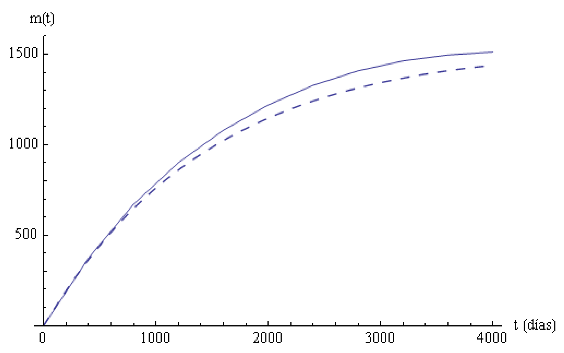
Columns 6, 7 in Table 4 are the empirical and estimated mean times until time t in the system. A linear regression model $Y=aX+b+\epsilon$ is applied to compare these mean values, with Y representing the estimated variable $n\left(t\right)$ and X the empirical variable $m\left(t\right)$. Parameter b is 0 since the initial point is $(0,0)$ for X and Y, and parameter a $\sim 0.9422$ with an adjusted determination coefficient $R^2=0.9999$; the p-value of the corresponding test is much smaller than $0.05$, and the fit cannot be rejected. In Figure 3, the two mean times in the systems are plotted.

Figure 3. Staying mean times in the system: empirical (continuous) and estimated (- -).

The longitudinal study of the survival times in states and in the system for the total of patients under bladder cancer considering a Markovian state-space model has been performed, the staying times are estimated and compared with the corresponding empirical values, and the fittings are acceptable in statistical terms. The survival function (Figure 2) and the mean times in states (Figure 3) illustrate the good fitting of these measures. A more detailed study, based on Figure 1, can be performed considering the well-differenced trajectories of the patients to the two absorbent states, and these present different characteristics that will be studied in the following sections. The notation of the present section is preserved. The diagram of transition among states presenting clearly the two trajectories in the disease is shown in Figure 1.

4. Patients with Progression

We consider the 52 patients undergoing progression and analyze the evolution with time. The transition diagram restricted to this group is given in Figure 4, and it follows a Coxian model under PH-distributions. The study is the one followed in Section 3 restricted to this sub-cohort, the procedure and calculations are as in the previous section, and the comments to the results will be given. We observe that $50\%$ of the patients enter progression from state 0, and 19 from state 1, and the transitions to progression from states $2,3$ are $4,3$, respectively. A total of $86.5\%$ of the patients reach progression from states $0,1$.

Figure 4. Transition diagram among the states.

The statistics associated with the staying time in states are given in Table 5.

Table 5. Empirical statistics of the staying times in states.

State	n	$\mathbf{Rang}$	$\mathbf{Min}$	$\mathbf{Max}$	$\mathbf{Med}$	$\mathbf{Mean}$	$\mathbf{sd}$
0	52	3878	92	3970	$250.00$	$453.77$	$640.33$
1	26	2261	87	2348	$284.50$	$525.08$	$559.21$
2	7	928	140	1068	$227.00$	$416.29$	$362.87$
3	3	2010	206	2216	$717.00$	$1046.33$	$1044.69$
System	52	3878	92	3970	$449.50$	$832.71$	$961.33$

As in the similar table for the total of patients, the dispersion of the measures is high, and the fit to the staying time in states is not good for the usual distributions, and the PH distributions solve this problem.

4.1. Survival Function

The empirical survival function $S_{\left(P\right)emp}$ is directly calculated from the dataset.

For calculating the survival function $S_{\left(P\right)}\left(t\right)$, PH distributions are fitted to the empirical staying times in states, and all of them are of order two:

$${\alpha }_0=(1,0)A_0=\left(\begin{array}{cc}-0.0159& 0.0159\\ 0.0010& -0.0037\end{array}\right)A_0^0=\left(\begin{array}{c}0\\ 0.0027\end{array}\right)$$

$${\alpha }_1=(1,0)A_1=\left(\begin{array}{cc}-0.0166& 0.0166\\ 0.0011& -0.0034\end{array}\right)A_1^0=\left(\begin{array}{c}0\\ 0.0023\end{array}\right)$$

$${\alpha }_2=(1,0)A_2=\left(\begin{array}{cc}-0.0120& 0.0120\\ 0.0009& -0.0041\end{array}\right)A_2^0=\left(\begin{array}{c}0\\ 0.0032\end{array}\right)$$

$${\alpha }_3=(1,0)A_0=\left(\begin{array}{cc}-0.0120& 0.0120\\ 0.0004& -0.0015\end{array}\right)A_0^0=\left(\begin{array}{c}0\\ 0.0011\end{array}\right).$$

All these fitted functions cannot be rejected with the $0.05$ significance level using the Kolmogorov-Smirnov statistics.

Following the methodology in Section 3, the multistate Markov process governing the system is denoted by $\left\{X\right(t),t\ge 0\}$, with $X\left(t\right)$ the state occupied at time t, state space $\{0,1,2,3,P\}$, and P an absorbent one. Blocks $A,B$ have a similar interpretation to the previous section, and the generator takes the form

$$Q=\left(\begin{array}{cc}{A}_{8\times 8}& B_{8\times 1}\\ 0_{1\times 8}& 0_{1\times 1}\end{array}\right),$$

being $A,B$,

$$A=\left(\begin{array}{cccc}{A}_0& p_{0,1}{A}_0^0{\alpha }_1& & \\ & A_1& p_{1,2}{A}_1^0{\alpha }_2& \\ & & A_2& p_{2,3}{A}_2^0{\alpha }_3\\ & & & A_3\end{array}\right)B=\left(\begin{array}{c}{p}_{0,P}{A}_0^0\\ p_{1,P}{A}_1^0\\ p_{2,P}{A}_2^0\\ p_{3,P}{A}_3^0\end{array}\right).$$

Elements $p_{i,,j}$ are the proportion of patients of the transition $i\to j$, $i,j=1,2,3,P$; they satisfy $p_{i,(i+1)}+p_{i,P}=1$, $i=0,1,2$ and are obtained from Table 2. We have observed that half of the patients go to progression from state 0, and this number decreases with the following states, being very small from state 2. This can indicate that the treatment and the time receiving it significantly restricts the progression of the patients.

Once generator Q is calculated, matrix $P\left(t\right)$ of transition probability functions and the corresponding blocks $A\left(t\right),B\left(t\right)$, are obtained. The survival function is the probability of not occupying the absorbent state at time t:

$$S_{\left(P\right)}\left(t\right)=1-\alpha B\left(t\right).$$

(10)

The values of this function are calculated using a computational program. In Figure 5, these survival functions are plotted. The Kolmogorov-Smirnov test establishes that the fit must not be rejected with a significance level of $0.05$.

Figure 5. Empirical (continuous) and estimated (- -) survival functions.

4.2. Mean Times in States

The mean times in states for this group are calculated as in Section 3.4, and the notation is preserved. The numerical values for these means and for the system are given in Table 6.

Table 6. Staying mean times in states and in the system.

tk (Days)	$\begin{array}{c}{\mathit{m}}_0 \left(\mathit{t}\mathit{k}\right)\\ \mathbf{State}0\end{array}$	$\begin{array}{c}{\mathit{m}}_1 \left(\mathit{t}\mathit{k}\right)\\ \mathbf{State}1\end{array}$	$\begin{array}{c}{\mathit{m}}_2 \left(\mathit{t}\mathit{k}\right)\\ \mathbf{State}2\end{array}$	$\begin{array}{c}{\mathit{m}}_3 \left(\mathit{t}\mathit{k}\right)\\ \mathbf{State}3\end{array}$	$\begin{array}{c}\mathit{m} \left(\mathit{t}\mathit{k}\right)\\ \mathbf{System}\end{array}$	$\begin{array}{c}\mathit{n} \left(\mathit{t}\mathit{k}\right)\\ \mathbf{System}\end{array}$
400	$262.37$	$94.69$	0	0	312	$299.34$
800	$334.42$	$235.73$	$74.57$	143	$470.58$	$472.46$
1200	$368.06$	$317.73$	$174.86$	376	$575.31$	$581.39$
1600	$394.73$	$372.08$	$248.14$	$642.67$	$651.25$	$654.13$
2000	$412.92$	$418.23$	$305.29$	805	$709.58$	$704.54$
2400	$423.58$	$463.04$	$312.43$	$938.33$	$751.29$	$740.23$
2800	$431.27$	$482.50$	$369.57$	$1046.33$	$782.63$	$765.79$
3200	$438.96$	$497.88$	$416.29$	$1046.33$	$804.31$	$784.21$
3600	$446.65$	$513.27$	$416.29$	$1046.33$	$819.69$	$797.54$
4000	$453.77$	$525.08$	$416.29$	$1046.33$	$832.71$	$807.20$

The last two columns correspond to the empirical and estimated mean times. An analysis using the linear regression model among these functions, as it has been performed in the previous section is done maintaining the notation; variables $n\left(t\right),m\left(t\right):n\left(t\right)=am\left(t\right)+b+\epsilon$ are correlated with an adjusted determination coefficient $R^2=0.9999$ and coefficients $a\sim 0.94,b\sim 0,$ the p-value of the corresponding test is significant, and it is ∼$2\times {10}^{-16}.$ In Figure 6, these functions are plotted.

Figure 6. Staying mean times in the system: empirical (continuous) and estimated (- -).

The mean time of these patients in state 0 is about one year and three months; in state 1, it increases about two months, and, in state 2, it decreases to one year and one month and a half; the staying in state 3 is almost three years. The mean time in the system is two years and eleven weeks, according to the model, and two years and seven weeks, according to the empirical calculations.

It could be interesting to obtain information about some characteristics from the patients in this sub-cohort, such as treatments, to prevent this type of cancer by means of screening in the sub-population under risk. This information is not available by the authors.

5. Patients without Progression

The number of survivors to progression in the observation period is high. The transition diagram restricted to this group is given in Figure 7. The study is the one followed in Section 3 restricted to this sub-cohort, and, formally, it is the same as in Section 4. The notation is preserved. The set of states is $\{0,1,2,3,NP\}$. Sixty-three percent of the 795 patients in this group do not present recurrence in the observation period.

Figure 7. Transition diagram among the states.

In Table 7, the numerical values describing the mean values are given. As in similar tables in the analyzed cohorts, the data are disperse.

Table 7. Empirical statistics of the staying times in states.

State	n	$\mathbf{Rang}$	$\mathbf{Min}$	$\mathbf{Max}$	$\mathbf{Med}$	$\mathbf{Mean}$	$\mathbf{sd}$
0	795	4248	85	4333	$695.00$	$1004.85$	$883.94$
1	296	3887	95	3982	$404.50$	$693.12$	$679.58$
2	168	4009	83	4092	$375.50$	$637.58$	$668.99$
3	123	3192	82	3274	904	$1102.90$	$798.87$
$System$	795	4729	89	4818	$1275.00$	$1568.29$	$1129.48$

Again, the median is minor than the mean in the different states, the rang is similar to the one in the global system, and the dispersion is high; the usual distributions do not fit to the staying times in states, so PH distributions are fitted.

5.1. Survival Probability

In Figure 7, it is observed that nearly $63\%$ of the patients leave the system from state 0, and $37\%$ from the following states: nearly $43\%$ from state 1, nearly $23\%$ from state 2, and the remaining 123 patients reach the absorbent state $NP$. As in the previous section, the transitions follow a Coxian model.

The empirical survival function $S_{\left(NP\right)emp}$ is directly calculated from the dataset. For calculating the survival function $S\left(t\right)$ as in the previous model, PH distributions are fitted to the empirical staying times in states; in this case, not all the functions have the same order:

$${\alpha }_0=(1,0)A_0=\left(\begin{array}{cc}-0.0100& 0.0100\\ 0.0003& -0.0014\end{array}\right)A_0^0=\left(\begin{array}{c}0\\ 0.0011\end{array}\right)$$

$${\alpha }_1=(0,0,1,0)A_1=\left(\begin{array}{cccc}-0.0028& 0.0002& 0.0024& 0.0001\\ 0.0033& -0.0106& 0& 0.0073\\ 0.0001& 0.0106& -0.0107& 0\\ 0.0021& 0& 0& -0.0118\end{array}\right)A_1^0=\left(\begin{array}{c}0\\ 0\\ 0\\ 0.0097\end{array}\right)$$

$${\alpha }_2=(0,0.0118,0.9882)A_2=\left(\begin{array}{ccc}-0.0061& 0.0016& 0\\ 0.0001& -0.0021& 0.0020\\ 0.0060& 0.0001& -0.0061\end{array}\right)A_2^0=\left(\begin{array}{c}0.0044\\ 0\\ 0\end{array}\right)$$

$${\alpha }_3=(0.7813,0.2187)A_3=\left(\begin{array}{cc}-0.0016& 0.0016\\ 0& -0.0016\end{array}\right)A_0^0=\left(\begin{array}{c}0\\ 0.0016\end{array}\right).$$

The fits are not rejected with a significance level of $0.05$ in the Kolmogorov-Smirnov test. The survival times in the partition points are given in Table 8.

Table 8. Staying mean times in states and in the system.

tk (Days)	$\begin{array}{c}{\mathit{m}}_0 \left(\mathit{t}\mathit{k}\right)\\ \mathbf{State}0\end{array}$	$\begin{array}{c}{\mathit{m}}_1 \left(\mathit{t}\mathit{k}\right)\\ \mathbf{State}1\end{array}$	$\begin{array}{c}{\mathit{m}}_2 \left(\mathit{t}\mathit{k}\right)\\ \mathbf{State}2\end{array}$	$\begin{array}{c}{\mathit{m}}_3 \left(\mathit{t}\mathit{k}\right)\\ \mathbf{State}3\end{array}$	$\begin{array}{c}\mathit{m} \left(\mathit{t}\mathit{k}\right)\\ \mathbf{System}\end{array}$	$\begin{array}{c}\mathit{n} \left(\mathit{t}\mathit{k}\right)\\ \mathbf{System}\end{array}$
400	$349.06$	$71.57$	$15.32$	$0.00$	$378.94$	$377.66$
800	$571.91$	$216.86$	$106.83$	$57.91$	$684.18$	$686.87$
1200	$718.03$	$346.49$	$206.21$	$206.79$	$922.62$	$929.36$
1600	$821.66$	$441.52$	$306.47$	$372.79$	$1108.49$	$1114.14$
2000	$893.76$	$520.26$	$386.81$	$546.50$	$1253.76$	$1251.08$
2400	$944.57$	$584.90$	$459.99$	$693.15$	$1366.79$	$1350.07$
2800	$976.94$	$626.73$	$523.55$	$832.89$	$1449.79$	$1420.11$
3200	$995.36$	$654.50$	$574.86$	$942.97$	$1506.42$	$1468.77$
3600	$1002.80$	$636.42$	$602.57$	$1028.37$	$1540.71$	$1502.05$
4000	$1004.23$	$686.68$	$622.01$	$1070.98$	$1557.05$	$1524.52$

The multistate Markov process governing the system is denoted by $\left\{X\right(t),t\ge 0\}$, with $X\left(t\right)$ the state occupied at time t, state space $\{0,1,2,3,NP\}$ and $NP$ an absorbent one. Blocks $A,B$, have a similar interpretation to the previous section, and the generator takes the form

$$Q=\left(\begin{array}{cc}{A}_{11\times 11}& B_{11\times 1}\\ 0_{1\times 11}& 0_{1\times 1}\end{array}\right),$$

with

$$A=\left(\begin{array}{cccc}{A}_0& p_{0,1}{A}_0^0{\alpha }_1& & \\ & A_1& p_{1,2}{A}_1^0{\alpha }_2& \\ & & A_2& p_{2,3}{A}_2^0{\alpha }_3\\ & & & A_3\end{array}\right)B=\left(\begin{array}{c}{p}_{0,NP}{A}_0^0\\ p_{1,NP}{A}_1^0\\ p_{2,NP}{A}_2^0\\ p_{3,NP}{A}_3^0\end{array}\right).$$

The quantities $p_{i,,j}$ are the proportion of patients of the transition $i\to j$, $i,j=1,2,3,NP$; they satisfy $p_{i,(i+1)}+p_{i,NP}=1$, $i=0,1,2$ and are obtained from Table 2. The transition rate between consecutive states decreases, except in state 3. We can see that the trend to transitions in the transient states increases: $p_{0,1}<$ $p_{1,2}<p_{2,3}$, while the trend to survival (state $NP$) from states $0,1,2$ decreases.

Once generator Q is calculated, matrix $P\left(t\right)$ of transition probability functions and the corresponding blocks $A\left(t\right),B\left(t\right)$, are obtained. The survival function is the probability of not occupying the absorbent state at time t:

$$S_{\left(NP\right)}\left(t\right)=1-\alpha B\left(t\right).$$

(11)

In Figure 8, these functions are plotted. The Kolmogorov-Smirnov test establishes that the fit must not be rejected with a significance level of $0.05$.

Figure 8. Empirical (continuous) and estimated (- -) survival functions.

5.2. Mean Time in States

The mean times in states for this group are calculated as in Section 3.4, and the notation is preserved. The numerical values for these means and for the system are given in Table 8.

The last two columns correspond to the empirical and theoretical mean times, and we can see that the values are very similar. An analysis using the linear regression model among these functions as it has been performed in the previous section is done maintaining the notation; variables $n\left(t\right),m\left(t\right):n\left(t\right)=am\left(t\right)+b+\epsilon$ are correlated with an adjusted determination coefficient $R^2=0.9999$ and coefficients $a\sim 0.99,b\sim 0,$ the p-value of the corresponding test is significant, and it is ∼$2\times {10}^{-16}.$ In Figure 9, these functions are plotted.

Figure 9. Staying mean times in the system: empirical (continuous) and estimated (- -).

The mean time of these patients in state 0 is about two years and nine months; in states $1,2$, the means are similar, between two years and a half and three years; in state 3, it is almost three years. These quantities contribute to valuate the treatments. The mean time in the system is about four years and three months.

In this group of patients, we observe that the mean times in states 0 and 3 are similar, as well as higher than in states $1,2$. This fluctuations should be interpreted in terms of the treatments and the characteristics of the patients, information not available to the authors.

6. Conclusions

The study we present is centered in the temporal evolution of the bladder cancer. The longitudinal study allows description of how the number of patients in different stages changes with time and reveals the high difference among the two groups of patients, with or without progression, in the duration of the disease and, consequently, in the costs. Survival tables have been given for the total and the selected groups of patients, giving a general vision of the evolution of the disease. The methodology we propose can be applied to patients with different treatments, and it is possible to perform a more complete analysis of bladder cancer. It is particularly interesting to measure the effectivity of the treatments and a comparison among them, in order to improve the wellness of the patients. It is our interest to continue the study incorporating these new elements to the state-space model and to perform a deeper study of the cancer. The procedure can also be appropriate in other diseases.

A major novelty of this paper is to consider non-exponential random times of occupying the states. In general, the staying times in states are not exponential, mainly when the trajectories of the patients depend on the previous times and, consequently, the transition rates among states are not constant. This difficulty has been avoided considering the PH distributions as the basic tool in the study of the times, and it results to be a suitable model for analyzing the temporal measures. All this is done preserving the Markovian structure of the stochastic process governing the system; in return, the number of exponential phases enlarges the orders of the involved matrices. The expressions are presented in an algorithmic form for being computational implemented. The fits of the different quantities and functions between the empirical and estimated ones are good.

In biomedical literature, the costs deserve special attention, and the treatment of diseases is an important point for governments, patients, and society. Particularly, bladder cancer has a long treatment. In 1991, it was the most expensive one in terms of the direct cost in US [1]. We present how the costs can be estimated and applied to data, when available, and incorporated to the model we have studied. The direct costs include the consumption of primary care resources, surgeries, and medicines in hospitals and for outpatients treatment (ambulatory). The indirect costs have to do with the decrease in productivity and the labor inactivity.

Given the structure of the model, the costs are associated with the occupied states for the patients. For every patient in state $j=0,1,2,3$, the direct mean cost at time t is denoted by $C{D}_j\left(t\right)$. The fixed mean cost associated with the initial state corresponds to the diagnosis, the previous treatment to the first surgery, and the surgery cost, and it is denoted by $C{F}_0.$ This is applicable to the following states, denoted by $C{F}_j$, $j=0,1,2,3$. After surgery, the costs of the treatments per unit time for every patient are denoted by $CVj$. These are the direct costs. The mean time in state $j=0,1,2,3$ at time t has been denoted by $m_j\left(t\right)$.

The direct mean cost at time t in states can be expressed as:

$$C{D}_j\left(t\right)=C{F}_j+C{V}_j{m}_j\left(t\right)j=0,1,2,3.$$

(12)

The indirect cost per unit time in state j is denoted by $C{I}_j$, $j=0,1,2,3$. The total mean cost at time t of the trajectory of bladder cancer is:

$$CM\left(t\right)=\sum _{j=0}^{3}C{D}_j\left(t\right)+C{I}_j{m}_j\left(t\right)=\sum _{j=0}^{3}C{F}_j+\left[C{V}_j+C{I}_j\right]m_j\left(t\right).$$

(13)

A simulation of the costs has been carried out for the cohorts analyzed in the paper, and the mean numbers of staying times in states are very different for the two groups of patients and, consequently, the costs.

References

- Botteman, M.F.; Pashos, C.L.; Redaelli, A.; Laskin, B.; Hauser, R. The Health Economics of Bladder Cancer. Pharmaeconomics 2003, 7, 1315–1330. [Google Scholar]
- Grasso, M. Bladder cancer: A major public health issue. Eur. Urol. Suppl. 2008, 7, 510–515. [Google Scholar] [CrossRef]
- Bosetti, C.; Bertuccio, P.; Chatenoud, L.; Negri, E.; Vecchia, C.L.; Levi, F. Trends in mortality from urologic cancers in Europe 1970–2008. Eur. Urol. J. 2011, 60, 1–15. [Google Scholar] [CrossRef]
- Antoni, S.; Ferlay, J.; Soerjomataram, I.; Znaor, A.; Jemaol, A.; Bray, F. Bladder Cancer Incidence and Mortality: Global Overview and Recent Trends. Eur. Urol. 2017, 71, 96–108. [Google Scholar] [CrossRef]
- Cox, D.R. Regression models and life tables (with discussion). J. R. Stat. Soc. Ser. B 1972, 34, 187–220. [Google Scholar]
- García, B.; Rubio, G.; Santamaría, C. A Predictive Mathematical Model in the Recurrence of Bladder Cancer. Math. Comput. Model. 2005, 42, 621–634. [Google Scholar]
- García-Mora, B.; Santamaría, C.; Rubio, G.; Pontones, J.L. Modeling the recurrence–progression process in bladder carcinoma. Comput. Math. Appl. 2008, 56, 619–630. [Google Scholar] [CrossRef]
- Andersen, P.K.; Gill, R.D. Cox’ regression model for counting processes: A large sample study. Ann. Stat. 1982, 10, 1100–1120. [Google Scholar] [CrossRef]
- Amorim, L.D.; Cai, J. Modelling recurren events: A tutorial for analysis in epidemiology. Int. J. Epidemiol. 2015, 44, 324–333. [Google Scholar]
- Geskus, R.B. Data Analysis with Competing Risks and Intermediate States; Chapman & Hall: Boca Raton, FL, USA, 2016. [Google Scholar]
- Andersen, P.K.; Keiding, N. Multi-state models for event history analysis. Stat. Methods Med. Res. 2002, 11, 91–115. [Google Scholar] [CrossRef]
- Porta, N.; Calle, M.L.; Malats, C.; Gómez, G. A dynamic model for the risk of bladder cancer progression. Stat. Med. 2012, 31, 287–300. [Google Scholar] [CrossRef] [PubMed]
- Beyer, U.; De Jardin, D.; Meller, M.; Rufibach, K.; Burger, J.U. A multistate model for early decision-making in oncology. Biom. J. 2020, 62, 550–567. [Google Scholar] [CrossRef] [PubMed]
- Aalen, O.O.; Cook, R.J.; Roysland, K. Does Cox analysis of a randomized survival study yield a causal treatment effect? Lifetime Data Anal. 2015, 21, 579–593. [Google Scholar] [CrossRef] [PubMed]
- Cook, R.J.; Lawless, J.F. Analysis of repeated events. Stat. Methods Med. Res. 2012, 11, 141–166. [Google Scholar] [CrossRef]
- Kay, R.A. Markov model for analysing cancer markers and disease states in survival studies. Biometrics 1986, 42, 855–865. [Google Scholar] [CrossRef]
- Pérez-Ocón, R.; Ruiz-Castro, J.E.; Gámiz-Pérez, M.L. A Multivariate Model to Measure the Effect of Treatments in Survival to Breast Cancer. Biom. J. 1998, 40, 703–715. [Google Scholar] [CrossRef]
- Pérez-Ocón, R.; Ruiz-Castro, J.E. A Multiple-Absorbent Markov Process in Survival Studies: Application to Breast Cancer. Biom. J. 2003, 45, 1–15. [Google Scholar] [CrossRef]
- Santamaría, C.; García-Mora, B.; Rubio, G.; Navarro, E. A Markov model for analyzing the evolution of bladder carcinoma. Math. Comput. Model. 2009, 50, 726–732. [Google Scholar]
- Pérez-Ocón, R.; Ruiz-Castro, J.E.; Gámiz-Pérez, M.L. Markov Models with Lognormal Transition Rates in the Analysis of Survival Times. Test 2000, 9, 353–370. [Google Scholar] [CrossRef]
- Pérez-Ocón, R.; Ruiz-Castro, J.E.; Gámiz-Pérez, M.L. A piecewise Markov process for analyzing survival from breast cancer in different risk groups. Stat. Med. 2001, 20, 109–122. [Google Scholar] [CrossRef]
- Pérez-Ocón, R.; Ruiz-Castro, J.E.; Gámiz-Pérez, M.L. Nonhomogeneous Markov Models in the Analysis of Survival after Breast Cancer. J. R. Stat. Soc. C 2001, 50, 111–124. [Google Scholar] [CrossRef]
- Ruiz-Castro, J.E.; Pérez-Ocón, R. Semi-Markov model in biomedical studies. Commun. Stat. Theory Methods 2004, 33, 437–455. [Google Scholar] [CrossRef]
- Wang, X.; Pai, J.S.; Shand, K.J. A semi-Markov model of disease recurrence in insured dogs. Appl. Stoch. Model. Bus. Ind. 2007, 23, 429–437. [Google Scholar] [CrossRef]
- Limnios, N. Reliability Measures of Semi-Markov Systems with General State Space. Methodol. Comput. Appl. Probab. 2012, 14, 895–917. [Google Scholar] [CrossRef]
- Neuts, M.F. Matrix-Geometric Solutions in Stochastic Models—An Algorithmic Approach; The John Hopkins University Press: Baltimore, MD, USA, 1981. [Google Scholar]
- Asmussen, S.; Nerman, O.; Olsson, M. Fitting phase-type distribution via the EM algorithm. Scand. J. Probab. 1996, 23, 419–441. [Google Scholar]
- Aalen, O.O. Phase Type Distributions in Survival Analysis. Scand. J. Stat. 1995, 22, 447–463. [Google Scholar]
- García-Mora, B.; Santamaría, C.; Ruiz, G. A Phase-Type Distribution for the Sum of Two Concatenated Markov Processes Application to the Analysis Survival in Bladder Cancer. Mathemathics 2020, 8, 2099. [Google Scholar]
- Marshall, A.H.; McClean, S. Using Coxian Phase-Type Distributions to Identify Patient Characteristics for Duration of Stay in Hospital. Health Care Manag. Sci. 2004, 7, 285–298. [Google Scholar] [CrossRef]
- Garg, L.; McClean, S.; Meenan, B.J.; Millard, P. Phase-Type Survival Trees and MIxed Distribution Survival Trees for Clustering Patient’s Hospital Length of Stay. Informatica 2011, 22, 57–72. [Google Scholar] [CrossRef]
- Donnelly, C.; McFetridge, M.; Marshall, A.H.; MItchell, H.J. A two-stage approach to the joint analysis of longitudinal and survival data utilizing the Coxian phase-type distribution. Stat. Methods Med. Res. 2018, 27, 3577–3594. [Google Scholar] [CrossRef] [PubMed]
- Distefano, S.; Longo, F.; Trivedi, K.S. Investigating dynamic reliability and availability through state-space models. Comput. Math. Appl. 2012, 64, 3701–3716. [Google Scholar] [CrossRef]
- Asmussen, S. Matrix-analyticc Models and their Analysis. Scand. J. Stat. 2000, 27, 193–226. [Google Scholar] [CrossRef]
- Luján, S. Modelización Matemática de la Multirrecidiva y Heterogeneidad Individual Para el Cálculo del Riesgo Biológico de Recidiva y Progresión del Tumor Vesical no Músculo Invasivo. Ph.D. Thesis, Universitat de València, València, Spain, 2012. (In Spanish). [Google Scholar]
Publisher’s Note: MDPI stays neutral with regard to jurisdictional claims in published maps and institutional affiliations. |
© 2021 by the authors. Licensee MDPI, Basel, Switzerland. This article is an open access article distributed under the terms and conditions of the Creative Commons Attribution (CC BY) license (http://creativecommons.org/licenses/by/4.0/).