Iterative Variable Selection for High-Dimensional Data: Prediction of Pathological Response in Triple-Negative Breast Cancer

Abstract

Over the last decade, regularized regression methods have offered alternatives for performing multi-marker analysis and feature selection in a whole genome context. The process of defining a list of genes that will characterize an expression profile remains unclear. It currently relies upon advanced statistics and can use an agnostic point of view or include some a priori knowledge, but overfitting remains a problem. This paper introduces a methodology to deal with the variable selection and model estimation problems in the high-dimensional set-up, which can be particularly useful in the whole genome context. Results are validated using simulated data and a real dataset from a triple-negative breast cancer study.

1. Introduction

Breast cancer (BC) is the most frequent cancer among women, representing around 25% of all new cancer diagnoses in women [1]. One in eight women in developed countries will be diagnosed with BC over the course of a lifetime.

The prognosis of this disease has progressively improved over the past three decades, due to the implementation of population-based screening campaigns and, above all, the introduction of new effective targeted medical therapies, i.e., aromatase inhibitors (effective in hormone receptor-positive tumors) and trastuzumab (effective in HER2-positive tumors). Breast cancer is, however, a heterogeneous disease. The worst outcomes are associated with the so-called triple-negative breast cancer subtype (TNBC), diagnosed in 15–20% of BC patients. TNBC is defined by a lack of immunohistochemistry expression of the estrogen and progesterone receptors and a lack of expression/amplification of HER2 [2]. The absence of expression of these receptors makes chemotherapy the only available therapy for TNBC.

TNBC is usually diagnosed in an operable (early) stage. Surgery, chemotherapy and radiation therapy are the critical components of the treatment of early TNBC. Many early TNBC patients are treated with upfront chemotherapy (neoadjuvant chemotherapy, NACT) and then operated on and, perhaps, irradiated. The rationale for this sequence is the ability to predict the long-term outcome of patients looking at the pathological response achieved with initial NACT [3].

With the currently available neoadjuvant chemotherapy regimens, nearly 50% of TNBC patients achieve a good pathological response to this therapy, whereas the remaining patients have an insufficient response. TNBC patients achieving a complete or almost complete disappearance of the tumor in the breast and axilla after NACT have an excellent outcome (less than 10% of relapses at five years), in contrast with those with significant residual disease (more than 50% of relapses at five years) [4,5].

The identification of these two different populations is therefore of utmost relevance, in order to test new experimental therapies in the population unlikely to achieve a good pathological response.

Several tumor multigene predictors of pathological response of operable BC to NACT have been proposed over the past few years, taking advantage of the recent decreased economic cost of obtaining an individual’s full transcriptome [6,7,8]. Most of them have been tested in unselected populations of BC patients and have shown insufficient positive predictive value and sensitivity.

The process of defining a list of genes that will define a characteristic expression profile is still ambiguous. This process relies upon advanced statistics and can use an agnostic point of view or include some a priori knowledge, but overfitting remains a problem. RNA-Seq has become one of the most appealing tools of modern whole transcriptome analyses because it combines a relatively low cost and a comprehensive approach to transcript quantification. Some approaches to complex disease biomarker discovery already pointed to the need to use a whole genome perspective using joint information in order to predict complex traits instead of a priori selecting individual features [9,10]. This strategy would lead to high predictive accuracy, and there would be no need to know the precise biological associations in the genome background because of the high correlation among the biomarkers [11]. This approach is challenging from the statistical point of view because of the large number of biomarkers that must be tested along the genome in relation to the rather small sample sizes in clinical studies. On the other hand, daily clinical practice scenarios require cheaper and faster quantification platforms than whole-genome RNA-Seq analysis. Thus, it is necessary to reduce the number of biomarkers to focus on in order to define a practical gene expression signature for the clinical community.

Regularized regression methods provide alternatives for performing multi-marker analysis and feature selection in a whole genome context [12]. Specifically, we focus on the sparse-group lasso (SGL) regularization method [13], which generalizes lasso [14], group lasso [15] and elastic-net [16], merging lasso and group lasso penalties. The solution provided by SGL usually involves a small number of predictor variables, given that many coefficients in the solution are exactly zero. It has an advantage over lasso when the predictor variables are grouped, as many groups are entirely zeroed out, but unlike group lasso, the solution is also sparse within those groups that are not completely eliminated from the model. However, as will be explained in the next sections, the SGL is not appropriate for the problem we are dealing with without introducing a broader methodology to control the regularization hyper-parameters, the groups, and the high-dimensionality issue. From a methodological point of view, this paper provides an original contribution to perform variable selection and model fitting in high-dimensional problems, allowing a priori selection of the final number of variables and addressing the problem of overfitting with the introduction of the importance index. Furthermore, the results presented in this paper are the first attempt in a translational oncology scenario at building a predictive model for the response to treatment, based entirely on whole genome RNA-Seq data and conventional clinical variables.

This paper is organized as follows. Section 2 ties together the various theoretical concepts that support our approach. Section 2.1 introduces the mathematical formulation of the SGL as an optimization problem. Section 2.2 discusses the iterative-sparse group lasso, a coordinate descent algorithm used to automatically select the regularization parameters of the SGL. Section 2.3 describes a clustering strategy for the variables, based on principal component analysis, which makes it possible to work with an arbitrarily large number of variables without specifying the groups a priori. Section 2.5 highlights our main methodological contributions: the importance and the power indexes, to weight variables and models, respectively. In Section 3, a simulation study is presented, with several synthetic matrix designs, and varying the number of variables from 40 to 4000. Section 4 highlights the contributions of our methodology on a TNBC cohort that had undergone neoadjuvant docetaxel/carboplatin chemotherapy. Some conclusions and outlines for future work are drawn in the final section.

2. Methodology and Algorithms

Consider the usual logistic regression framework, with N observations in the form $\{y^{\left(i\right)}$, $x_1^{\left(i\right)}$, $x_2^{\left(i\right)},\dots ,x_p^{\left(i\right)}{\}}_{i=1}^N$, where p is the number of features or predictor variables, and $y^{\left(i\right)}$ is the binary response. We assume that the response comes from a random variable with conditional distribution,

$$Y|(X_1\dots X_p)\sim Ber\left(p(X_1\dots X_p,\mathbf{\beta })\right),$$

where:

$$p(X_1\dots X_p,\mathbf{\beta })={(1+exp(-\eta ))}^{-1},$$

and $\eta$ is the linear predictor,

$$\eta ={\beta }_0+\sum _{j=1}^p{\beta }_j{X}_j,\mathbf{\beta }=[{\beta }_0{\beta }_1\dots {\beta }_p]\in {\mathbb{R}}^{p+1}.$$

The objective is to predict the response Y for future observations of $X_1\dots X_p$, using an estimation of the unknown parameter $\mathbf{\beta }$, given by:

$$\widehat{\mathbf{\beta }}=\underset{\mathbf{\beta }\in {\mathbb{R}}^{p+1}}{argmin}\widehat{R}\left(\mathbf{\beta }\right),$$

(1)

where:

$$\widehat{R}\left(\mathbf{\beta }\right)=\frac{1}{N}\sum _{i=1}^N\left[log\left(1+exp\{{\beta }_0+\sum _{j=1}^p{\beta }_j{x}_j^{\left(i\right)}\}\right)-y_i({\beta }_0+\sum _{j=1}^p{\beta }_j{x}_j^{\left(i\right)})\right].$$

(2)

The problem with this approach is that for $N<p$, the minimization (1) has infinite optimal solutions. When the features $X_1\dots X_p$ represent genetic expressions, this problem of predicting Y becomes more extreme, since we often have N several orders of magnitude smaller than p.

As a solution, variable selection techniques are proposed, in order to tackle the analytical intractability of this problem.

2.1. The Sparse-Group Lasso

It has been shown that SGL can play an important role in addressing the issue of variable selection in genetic models, where genes are grouped following different pathways. The mathematical formulation of this problem is:

$$\widehat{\mathbf{\beta }}\left(\mathbf{\lambda }\right)=\underset{\mathbf{\beta }\in {\mathbb{R}}^{p+1}}{argmin}\left\{\widehat{R}\left(\mathbf{\beta }\right)+{\lambda }_2\sum _{j=1}^J{\gamma }_j\parallel {\mathbf{\beta }}^{\left(j\right)}{\parallel }_2+{\lambda }_1{\parallel \mathbf{\beta }\parallel }_1\right\}.$$

(3)

Here J is the number of groups, ${\mathbf{\beta }}^{\left(j\right)}\in {\mathbb{R}}^{p_j}$ are vectors with the components of $\mathbf{\beta }$ corresponding to j-th group (of size $p_j$), and ${\gamma }_j=\sqrt{p_j}$, $j=1,2,\dots ,J$. The regularization parameter is $\mathbf{\lambda }=\left[{\lambda }_1{\lambda }_2\right]\in {\mathbb{R}}_{+}^2.$

The problem with (3) is that the vector $\widehat{\mathbf{\beta }}\left(\mathbf{\lambda }\right)$ of estimated coefficients depends on the selection of a vector of regulation parameters $\mathbf{\lambda }$, which must be chosen before estimating $\widehat{\mathbf{\beta }}\left(\mathbf{\lambda }\right)$. The selection of $\mathbf{\lambda }$ is partly an open problem, because although there are several practical strategies for choosing these parameters, there is no established theoretical criterion to follow. In most cases, the regularization parameters are set a priori, based on some additional information about the data, or the characteristics of the desired solution, e.g., a greater ${\lambda }_1$ implies that more components of $\widehat{\mathbf{\beta }}$ are identically zero. The most commonly used methodology to select $\mathbf{\lambda }$ consists of moving the regulation parameters in a fixed grid, which is usually not very thin. However, this approach has many disadvantages. By contrast, we propose the iterative-sparse group lasso, a coordinate descent algorithm, recently introduced in [17].

2.2. Selection of the Optimal Regularization Parameter

Traditionally, the data set $\mathcal{Z}={\{y^{\left(i\right)},x_1^{\left(i\right)},x_2^{\left(i\right)},\dots ,x_p^{\left(i\right)}\}}_{i=1}^N$ is partitioned into three disjoint data sets, ${\mathcal{Z}}_T,{\mathcal{Z}}_V$, and ${\mathcal{Z}}_{test}$. The data in ${\mathcal{Z}}_T$ are used for training the model, i.e., solving (3). ${\mathcal{Z}}_V$ is used for validation, i.e., finding the optimal parameter $\mathbf{\lambda }$. The remaining observations in ${\mathcal{Z}}_{test}$ are used for testing the prediction ability of the model on future observations. Specifically, the selection of the optimal parameter $\mathbf{\lambda }$ is based on the minimization of the validation error, defined as:

$${\widehat{R}}_V\left(\mathbf{\lambda }\right)=\frac{1}{\#{\mathcal{Z}}_V}\sum _{(y^{(i)},{\mathbf{x}}^{(i)})\in {\mathcal{Z}}_V}\left[log(1+exp\{\eta ({\widehat{\mathbf{\beta }}}_T)\})-y^{\left(i\right)}\eta ({\widehat{\mathbf{\beta }}}_T)\right],$$

(4)

where:

$${\widehat{\mathbf{\beta }}}_T\left(\mathbf{\lambda }\right)=arg\underset{\mathbf{\beta }\in B}{min}\left\{{\widehat{R}}_T\left(\mathbf{\beta }\right)+{\lambda }_2\sum _{j=1}^J{\gamma }_j\parallel {\mathbf{\beta }}^{\left(j\right)}{\parallel }_2+{\lambda }_1{\parallel \mathbf{\beta }\parallel }_1\right\},$$

(5)

and:

$${\widehat{R}}_T\left(\mathbf{\beta }\right)=\frac{1}{\#{\mathcal{Z}}_T}\sum _{(y^{\left(i\right)},{\mathbf{x}}^{\left(i\right)})\in {\mathcal{Z}}_T}\left[log(1+exp\{\eta ({\widehat{\mathbf{\beta }}}_T)\})-y^{(i)}\eta ({\widehat{\mathbf{\beta }}}_T)\right],$$

(6)

with # denoting the cardinal of a set. Therefore, the problem of finding the optimal parameter $\mathbf{\lambda }$ can be formulated as:

$$\begin{array}{c}\underset{\mathbf{\lambda }\in {\mathbb{R}}_{+}^2}{min}{\widehat{R}}_V\left(\mathbf{\lambda }\right)\\ \mathrm{s}.\mathrm{t}.{\widehat{\mathbf{\beta }}}_T\left(\mathbf{\lambda }\right)=arg\underset{\mathbf{\beta }\in {\mathbb{R}}^{p+1}}{min}\left\{{\widehat{R}}_T\left(\mathbf{\beta }\right)+{\lambda }_2\sum _{j=1}^J{\gamma }_j\parallel {\mathbf{\beta }}^{\left(j\right)}{\parallel }_2+{\lambda }_1{\parallel \mathbf{\beta }\parallel }_1\right\}.\end{array}$$

(7)

Algorithm 1 describes the two-parameter iterative sparse-group lasso (isgl${}_0$), a gradient-free coordinate descent method to tune the parameter $\mathbf{\lambda }$ from the sparse-group lasso (3), which performs well under different scenarios while drastically reducing the number of operations required to find optimal penalty weight parameters that minimize the validation error in (4). The isgl${}_0$ iteratively performs a univariate minimization over one of the coordinates of $\mathbf{\lambda }$, while the other coordinate is fixed.

Algorithm 1: Two-parameter iterative sparse-group lasso (isgl${}_0$)

As mentioned before, a very useful property of the sparse-group lasso as a variable selection method is the ability to remove entire groups from the model (sending to zero the components of the $\widehat{\mathbf{\beta }}$ vector relative to those groups), as is the case with group lasso. However, this means that a grouping among the variables under consideration must be specified. This does not entail a challenge if there are natural groupings among the variables, e.g., if the variables are dummies related to different levels of the same original categorical variable. However, in our study most of the variables are transcriptomes, for which there are no established groupings in the literature. To overcome this problem, we suggest an empirical variable grouping approach, based on the principal component analysis of the data matrix.

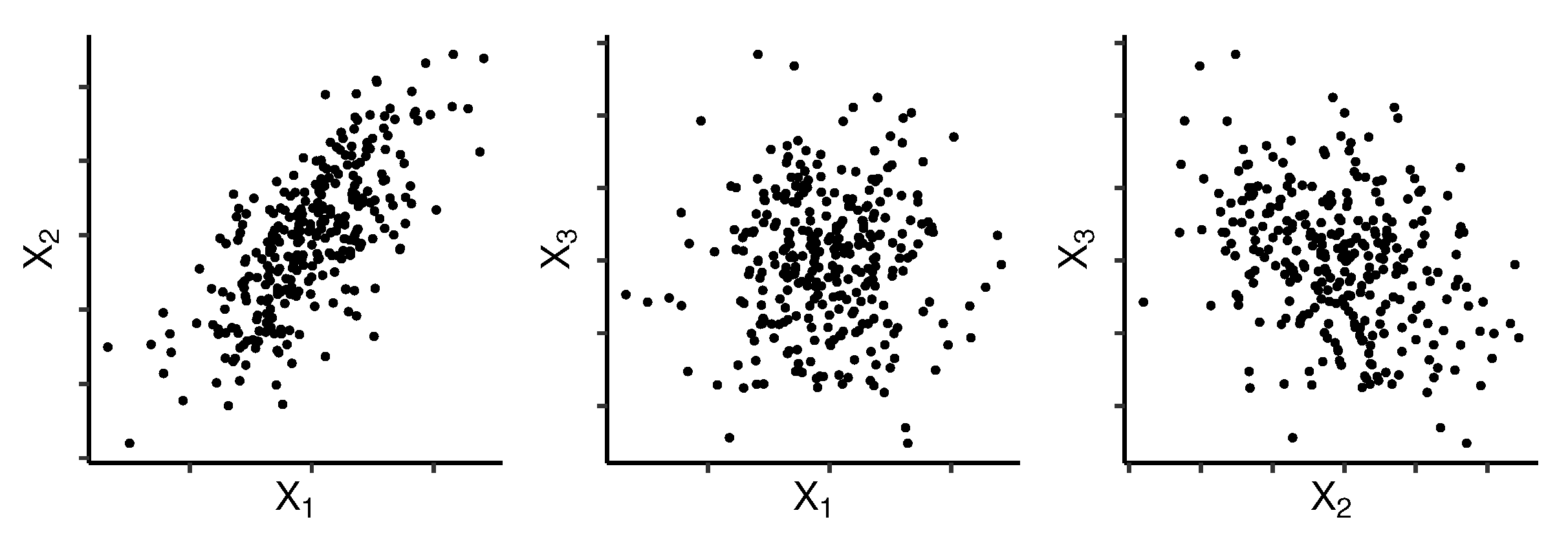
2.3. Grouping Variables Using Principal Component Analysis

Principal component analysis (PCA) is a dimension reduction technique, which is very effective in reducing a large number of variables related to each other to a few latent variables while trying to lose a minimum amount of information. The new latent variables obtained (the principal components), which are a linear transformation of the original variables, are uncorrelated and ordered in such a way that the first components capture most of the variation present in all of the original variables.

Given the data matrix $\mathbf{X}\in {\mathbb{R}}^{N\times p}$, PCA computes the rotation matrix $\mathbf{W}\in {\mathbb{R}}^{p\times G}$, where $G\le min(N,p)$ is the number of principal components to retain. The transformed data matrix (the principal component matrix) is $\mathbf{T}=\mathbf{X}\mathbf{W}$. This rotation matrix $\mathbf{W}$ suggests a natural grouping on the columns of $\mathbf{X}$, given by:

$$group\left(X_j\right)=arg\underset{i}{max}\left|W_{ji}\right|,j=1,2,\dots ,p.$$

(8)

This strategy will provide at most G groups on the columns of $\mathbf{X}$.

The following example illustrates our approach on a simulated data set. Suppose that we want to cluster variables $X_1,X_2$, and $X_3$ using two groups. There are 300 observations (Figure 1) and they are simulated such that $\mathrm{corr}(X_1,X_2)=0.75$, $\mathrm{corr}(X_1,X_3)=0.1$, and $\mathrm{corr}(X_2,X_3)=-0.25$. The principal components rotation matrix $\mathbf{W}$ is displayed in

Table 1. Principal components rotation matrix $\mathbf{W}$.

	PC1	PC2
$X_1$	−0.67	0.40
$X_2$	−0.70	−0.08
$X_3$	0.23	0.91

.

In this example, $X_1$ and $X_2$ would be grouped together, whereas $X_3$ would be in the other group. This method places highly correlated variables in the same group.

2.4. Mining Influent Variables under a Cross-Validation Approach

In this section, we focus on the problem of variable selection in models where the ratio $p/N$ is in the order of ${10}^2$. In these scenarios, even state-of-the-art methods such as SGL find it hard to select an appropriate set of variables related to the response term. We propose a cross-validation approach to fit and evaluate many different models using only a sample size of N initially given observations.

The solution in terms of $\widehat{\mathbf{\beta }}\left(\mathbf{\lambda }\right)$ provided by Algorithm 1 strongly depends on the partition ${\mathcal{Z}}_T,{\mathcal{Z}}_V$. As a consequence, if we run Algorithm 1 for different partitions ${\mathcal{Z}}_T,{\mathcal{Z}}_V$ of the same data $\mathcal{Z}$, it will probably result in different coefficient estimates $\widehat{\mathbf{\beta }}\left(\mathbf{\lambda }\right)$. Therefore, the indicator function of variable $X_j$ included in the model, $\mathbf{1}({\widehat{\beta }}_j\left(\mathbf{\lambda }\right)\ne 0)$, will take different values depending on the partition ${\mathcal{Z}}_T,{\mathcal{Z}}_V$. In order to avoid this dependency in the sample data partition, we propose Algorithm 2, which computes many different solutions $\widehat{\mathbf{\beta }}\left(\mathbf{\lambda }\right)$ of Algorithm 1 for different partitions of the original data sample $\mathcal{Z}$. The goal of this algorithm is to be able to fit and evaluate many models using the same data. Since the sample size is small compared to the number of covariates, the variable selection will greatly depend on the train–validate partition. We denote by R the total number of models that will be fitted using different partitions from the original sample. Algorithm 2 stores the information of the fitting $\widehat{\mathbf{\beta }}$ of each model and the correct classification rate in the validation sample ($cc{r}_V$) in each case.

Algorithm 2:

2.5. Selection of the Best Model

Our objective is to select one of the R models computed in Algorithm 2 to be our final model. We believe that a selection only based on the maximization of $cc{r}_V$ could lead to overfit in the training sample data $\mathcal{Z}$. To overcome this problem, we define two indexes: the importance index of a variable and the power of a model. These indexes are fundamental to choosing a final model that does not overfit the data.

We consider the importance index $I_j$ of variable $X_j$, defined as:

$$I_j=\sum _{r=1}^R|{\beta }_j^{\left(r\right)}|·(cc{r}_V^{\left(r\right)}-\delta )/\underset{j}{max}\left\{\sum _{r=1}^R|{\beta }_j^{\left(r\right)}|·(cc{r}_V^{\left(r\right)}-\delta )\right\},$$

(9)

where ${\mathbf{\beta }}^{\left(r\right)}$ and $cc{r}_V^{\left(r\right)}$ are those returned by Algorithm 2 on data $\mathcal{Z}$. With the objective of penalizing those models that performed poorly on the validation set, the term $\delta$ has been introduced, which is the maximum between $\overline{\mathit{y}}$ and $1-\overline{\mathit{y}}$, i.e., the null model correct classification rate.

The importance index weights each variable $X_1\dots X_p$ differently depending on the correct classification rate of the models in which each variable was present. The larger $I_j$, the greater the chances of $X_j$ being present in the underlying model that generated the data $\mathcal{Z}$.

Figure 2 illustrates the importance index, computed on a simulated data set, with $N=100$ observations and $p=400$ variables. Notice that the most important highest variables are actually in the generating model, and there is a clear gap in Figure 2 between them and the rest of the variables.

Based on the maximization of the importance index, an appropriate subset is selected from the original p variables. Although the true number of variables involved in the model is unknown, we can focus our attention on a predefined number of important variables K, which depends only on the sample data $\mathcal{Z}$. We empirically found $K=\lceil \sqrt{N/2}\rceil$ to achieve good results. Using the importance index of the best K variables, we define the power of a model as:

$$P_r=\frac{1}{{\sum }_{k=1}^K{I}_{\left(k\right)}}\sum _{j:I_j\le I_{\left(K\right)}}{I}_j|{\beta }_j^{\left(r\right)}|/\parallel {\mathbf{\beta }}^{\left(r\right)}{\parallel }_1,r=1,2\dots R,$$

(10)

where $I_{\left(k\right)}$ denotes the k-th greatest importance index, e.g., $I_{\left(1\right)}={max}_j{I}_j$. The power index P weights each model, depending on the importance of its included variables.

The selection of the final model is based on the criterion:

$$\widehat{\mathbf{\beta }}={\mathbf{\beta }}^{\left(r^{*}\right)},\mathrm{where}{r}^{*}=\underset{r}{max}\left\{P_r+cc{r}_V^{\left(r\right)}\right\}.$$

(11)

Equation (11), Algorithm 2, and the framework that supports them, are the main contribution of this paper from a methodological point of view. Equation (11) is based on the correct classification rates of R different fitted models, two indexes defined in this paper, and the iterative sparse-group lasso, which is a novel algorithm.

3. A Simulation Study

In this section, we illustrate the performance of Algorithm 2 using synthetic data. To generate observations, we have followed simulation designs from [13] (uncorrelated features) and [14,18,19] (correlated features). Since our objective was to evaluate Algorithm 2 in binary classification problems, we used a logistic regression model for the response term using the simulated design matrices in each case. We simulated data from the true model:

$$\mathbf{\eta }=\mathbf{X}\mathbf{\beta },$$

with the logistic response $\mathit{y}$ given by:

$$y_i\sim Ber\left(p_i\right),p_i={(1+exp(-{\eta }_i))}^{-1},i=1,2\dots N.$$

(12)

Five scenarios for $\mathbf{\beta }$ and $\mathbf{X}$ were simulated. In each example, our simulated data consisted of a training set of $N=50$ observations and p variables, and an independent test set of 5000 observations and p variables. Models were fitted using training data only. Below are the details of the five scenarios.

(SFHT_1)

$$\mathbf{\beta }=(1,2,3,4,5,\underset{p-5}{\underbrace{0,\dots ,0}})$$

and $X_i$ are i.i.d $N(0,1)$, for $1\le i\le p$.

(SFHT_2)

In this example, $\mathbf{\beta }$ is generated as in SFHT_1, but the rows of the model matrix $\mathbf{X}$ are i.i.d. generated from a multivariate gaussian distribution with $\mathrm{cov}(X_i,X_j)=0.5^{|i-j|},1\le j\le i\le p$.

(Tibs_1)

$$\mathbf{\beta }=(3,1.5,0,0,2,\underset{p-5}{\underbrace{0,\dots ,0}}),$$

and the rows of $\mathbf{X}$ are i.i.d. generated from a multivariate gaussian distribution with $\mathrm{cov}(X_i,X_j)=0.5^{|i-j|},1\le j\le i\le p$.

(Tibs_4)

$$\mathbf{\beta }=(\underset{10}{\underbrace{0,\dots ,0}},\underset{10}{\underbrace{2,\dots ,2}},\underset{10}{\underbrace{0,\dots ,0}},\underset{10}{\underbrace{2,\dots ,2}},\underset{p-40}{\underbrace{0,\dots ,0}})$$

and the rows of $\mathbf{X}$ are i.i.d. generated from a multivariate gaussian distribution with $\mathrm{cov}(X_i,X_j)=0.5$, and $\mathrm{var}\left(X_i\right)=1,1\le j<i\le p$.

(ZH_d)

$$\mathbf{\beta }=(\underset{15}{\underbrace{3,\dots ,3}},\underset{p-15}{\underbrace{0,\dots ,0}})$$

and the rows of $\mathbf{X}$ were generated as follows:

• $X_i=Z_1+{ϵ}_i^x,Z_1\sim N(0,1),i=1,\dots ,5,$
• $X_i=Z_2+{ϵ}_i^x,Z_2\sim N(0,1),i=6,\dots ,10,$
• $X_i=Z_3+{ϵ}_i^x,Z_3\sim N(0,1),i=11,\dots ,15,$
• $X_i\sim N(0,1)$, $X_i$ i.i.d. for $i=16,\dots ,p,$

where ${ϵ}_i^x$ are i.i.d. $N(0,0.01)$, for $1\le i\le 15$.

We aimed to investigate the robustness of our methodology in each example, measured using the test accuracy, as the number of noisy variables (not in the generating model) increased.

Table 2. Average correct classification rate ($ccr$, %) of Algorithm 2 (Alg. 2) in the test data (5000 observations), in 30 experiments for each configuration, and $N=50$ observations in the training sample. Mean standard errors are given in parenthesis. Algorithm 2 was run with $R=30$. To establish a baseline comparison, we also included Lasso with grid search (Lasso-GS), and our methodology with known groups.

	Simulation A
	p = 40	p = 100	p = 400	p = 1000	p = 4000
Alg. 2	77.82 (0.88)	73.97 (1.04)	65.42 (1.23)	62.1 (1.09)	56.95 (1.19)
Lasso (Grid Search)	82.61 (0.62)	81.1 (0.95)	83.08 (0.7)	83.48 (0.56)	84.27 (0.86)
Alg. 2 (Known Groups)	74.66 (1.24)	67.01 (1.8)	61.38 (1.8)	59.07 (1.49)	54.54 (1.19)
	Simulation B
	p = 40	p = 100	p = 400	p = 1000	p = 4000
Alg. 2	84.72 (0.65)	82.28 (0.99)	75.63 (1.14)	73.33 (1.55)	68.87 (1.46)
Lasso (Grid Search)	87.82 (0.57)	88.01 (0.67)	88.16 (0.65)	89.25 (0.43)	88.5 (0.49)
Alg. 2 (Known Groups)	80.36 (0.93)	81.57 (0.82)	75.72 (1.18)	74.98 (0.96)	69.48 (2.04)
	Simulation ZHa
	p = 40	p = 100	p = 400	p = 1000	p = 4000
Alg. 2	79.44 (0.76)	76.76 (0.87)	71.2 (0.86)	68.52 (1.08)	66.93 (1.46)
Lasso (Grid Search)	82.75 (0.79)	83.39 (0.6)	83.54 (0.41)	85.68 (0.42)	84.68 (0.45)
Alg. 2 (Known Groups)	78.72 (1.12)	75.75 (1.22)	70.81 (1.51)	69.54 (1.95)	61.98 (1.84)
	Simulation ZHc
	p = 40	p = 100	p = 400	p = 1000	p = 4000
Alg. 2	89.11 (0.3)	87.95 (0.38)	88 (0.52)	88.96 (0.54)	89.68 (0.4)
Lasso (Grid Search)	92.1 (0.43)	92.52 (0.55)	93.27 (0.34)	93.21 (0.35)	92.7 (0.38)
Alg. 2 (Known Groups)	83.98 (0.86)	83.11 (0.64)	81.12 (0.8)	81.81 (0.67)	81.52 (0.97)
	Simulation ZHd
	p = 40	p = 100	p = 400	p = 1000	p = 4000
Alg. 2	85.91 (0.81)	83.44 (0.87)	83.19 (0.81)	80.41 (1.16)	71.89 (1.51)
Lasso (Grid Search)	89.98 (0.63)	89.96 (0.86)	90.7 (0.5)	91.87 (0.6)	89.94 (0.98)
Alg. 2 (Known Groups)	79.79 (1.59)	75.55 (1.74)	68.4 (1.71)	62.58 (1.62)	55.93 (1.29)

describes the performance of the final model (Algorithm 2 with importance index) selected under our methodology in the scenarios described above. We have conducted 30 experiments in each case, as we varied the number of variables in the model (p). Mean standard errors are given in parenthesis. To establish a baseline comparison, we also included Lasso with grid search, and our methodology with groups known. Table 2 reveals that for all the configurations (except, perhaps Tibs_1 and SHFT_1) the methodology is very robust with respect to an increase in the number of variables p. In fact, for most of them, the $ccr$ does not vary much from $p=400$ to $p=1000$. Intuitively, the grouping strategy introduced in Section 2.3 places highly correlated variables in the same groups, producing better results when there is correlation between the variables in the model. That is why the simulation scheme SFHT_1 produces the poorest results. In SFHT_1, all the simulated variables are independent and therefore, there is not any clear way to group the variables.

From a computational point of view, however, Algorithm 2 is very expensive compared with lasso. In fact, the parameter R in Algorithm 2 is expected to linearly increase the computational burden of the method. That is because Algorithm 2 loops through R independent runs of Algorithm 1, which multiplies the computational cost of running one instance of Algorithm 1 by a factor R. However, the actual time needed to obtain a solution for Algorithm 2 can be decreased to the maximum of one instance of Algorithm 1, because this is a parallel problem. The remaining computations performed to select the best model can be ignored because they are at the same order of a matrix-vector product. Therefore, the parameter K is not going to affect the computational performance of our method. However, it should affect the predictive performance, since K is directly related to the model selection. Figure 3 compares the computational and predictive performance of our method and lasso on a numerical experiment. Figure 3 confirms that K does not affect the computational burden, and its impact on the predictive performance is also negligible in this case, although it has a peak when K equals the true number of variables in the generating model.

To empirically evaluate the impact of R, we propose a numerical simulation. Figure 4 displays the average elapsed time needed to obtain a solution to Algorithm 2 (Alg. 2) and lasso with grid search (lasso-GS), varying the parameter R (which does not affect lasso, which has been included as a baseline). The illustrated simulation design was ZH_d, with $n=50$ and $p=200$ both fixed, and R varying between 1 and 300. These experiments demonstrate that the relationship between R and the elapsed time is linear. In addition, Figure 4 confirms that we are trading computational cost for an increase of more than $10\%$ in the accuracy, which we believe is a reasonable trade for most applications.

4. Application to Biomedical Data

In this section, we evaluate the methodology described in Algorithm 2 with the model selection criterion given by (11) on a real case study. A sample of TNBC patients from a previously published clinical trial [20] was used to analyze relations between cancer cells’ transcriptome and the response of patients to the given medical treatment (docetaxel plus carboplatin). The dataset was composed of 93 observations (patients) and $16,616$ variables (genetic transcripts and clinical variables).

Figure 5 shows the highest 30 importance indexes out of a total of $16,616$ variables. The criterion used to measure the importance of the variables is given in (9). Algorithm 2 was run with $R=200$, and the cutoff value was set to $K=\lceil \sqrt{N/2}\rceil =7$, as described in Section 2.5. With this importance index, the power of each model was computed using (10) and the best model was chosen according to (11), as highlighted in Figure 6.

The selected model included 843 out of $16,616$ variables. The grouping strategy mentioned in Section 2.3 resulted in a total of 82 groups, from which 18 were included in the final model.

Figure 7 displays the distribution of the number of non-zero coefficients for each group that was included in the final model, which is revealing in several ways. Firstly, it indicates that PCA finds groups of similar lengths, and secondly, the selected model is sparse at both the group and the variable levels.

In an attempt to discover the biological and genetic meaning in the model selected by our methodology, we ran DAVID [21,22] to detect enriched functional-related gene groups. The clustering and functional annotation was performed using the default analysis options, and the role of the potential multiple testing effect was considered using the false discovery rate (FDR). The results are detailed in supplementary Table S1.

We observed just two remarkable families of pathways after the gene enrichment analysis: the homeobox-related and the oxidative phosphorylation pathways. They are both involved in the mechanism of action of docetaxel and carboplatin in response to the provided treatment.

The homeobox genes have been proposed to be involved in mechanisms of resistance to taxane-based oncologic treatments in ovarian and prostate cancer [23,24,25,26]. Docetaxel hyper-stabilizes the microtube structure, irreversibly blocking the cytoskeleton function in the mitotic process and intracellular transport. In addition, this drug induces programmed cell death.

On the other hand, carboplatin attaches alkyl groups to DNA bases, resulting in fragmentation by repair enzymes when trying to repair them. It also inducts to mutations due to nucleotide despairing and generates DNA cross-links that affects the transcription process [27]. The development of resistance to platinum-based schemes of chemotherapy is a common feature. Several studies demonstrate that dysfunctions in mitochondrial processes, in conjunction with the mentioned mechanism of action, can contribute to the development of phenotypes associated with resistance [28,29,30,31,32,33].

5. Conclusions

The present study introduced a methodology to deal with the variable selection problem in a high dimensional set-up. It can be seen as an extension of the sparse-group lasso regularization method, without dependencies on both the hyper-parameters and the groups. There are several critical components in this approach:

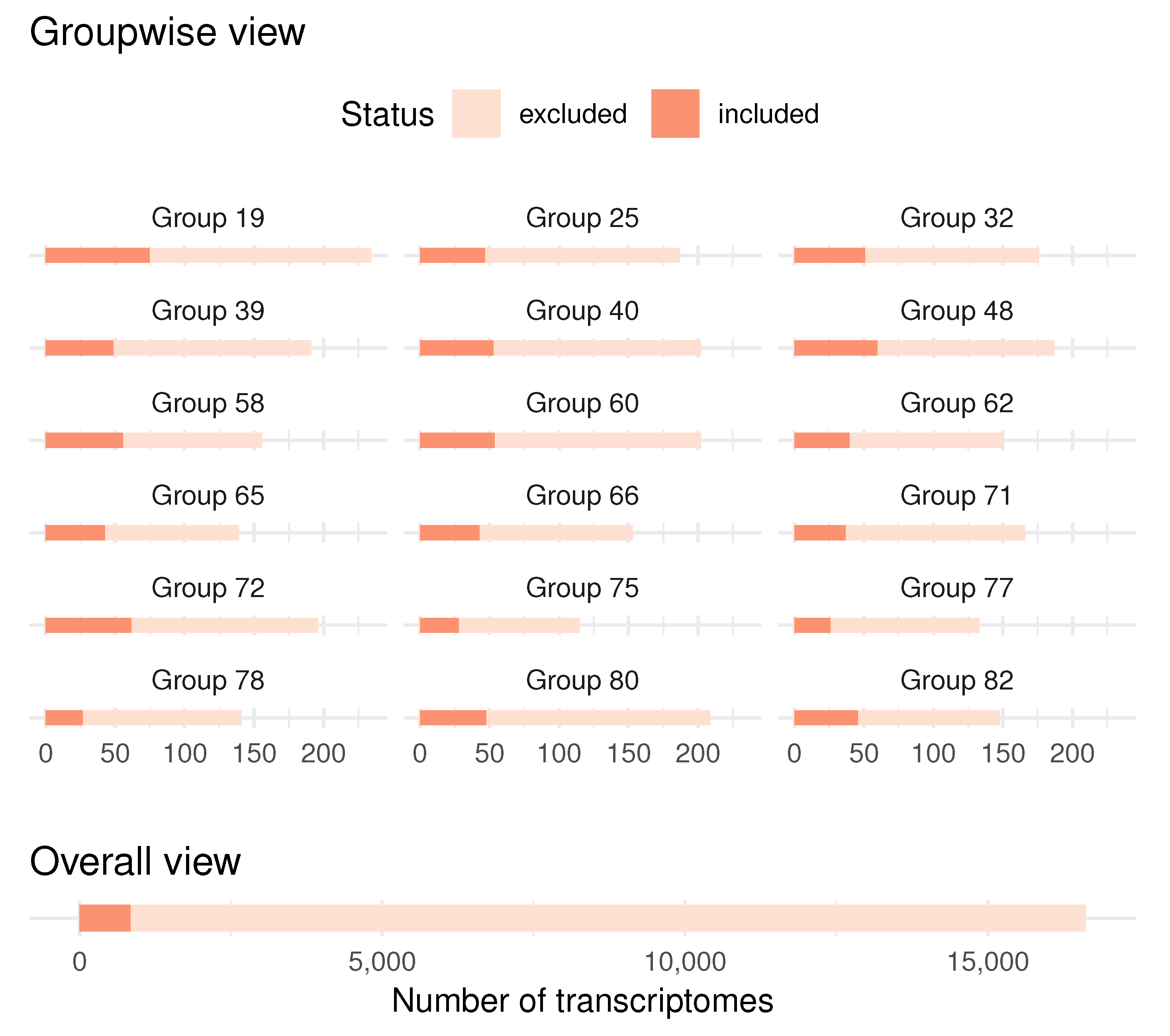
• A clustering of the variables, based on PCA, makes it possible to work with an arbitrarily large number of variables without specifying groups a priori.
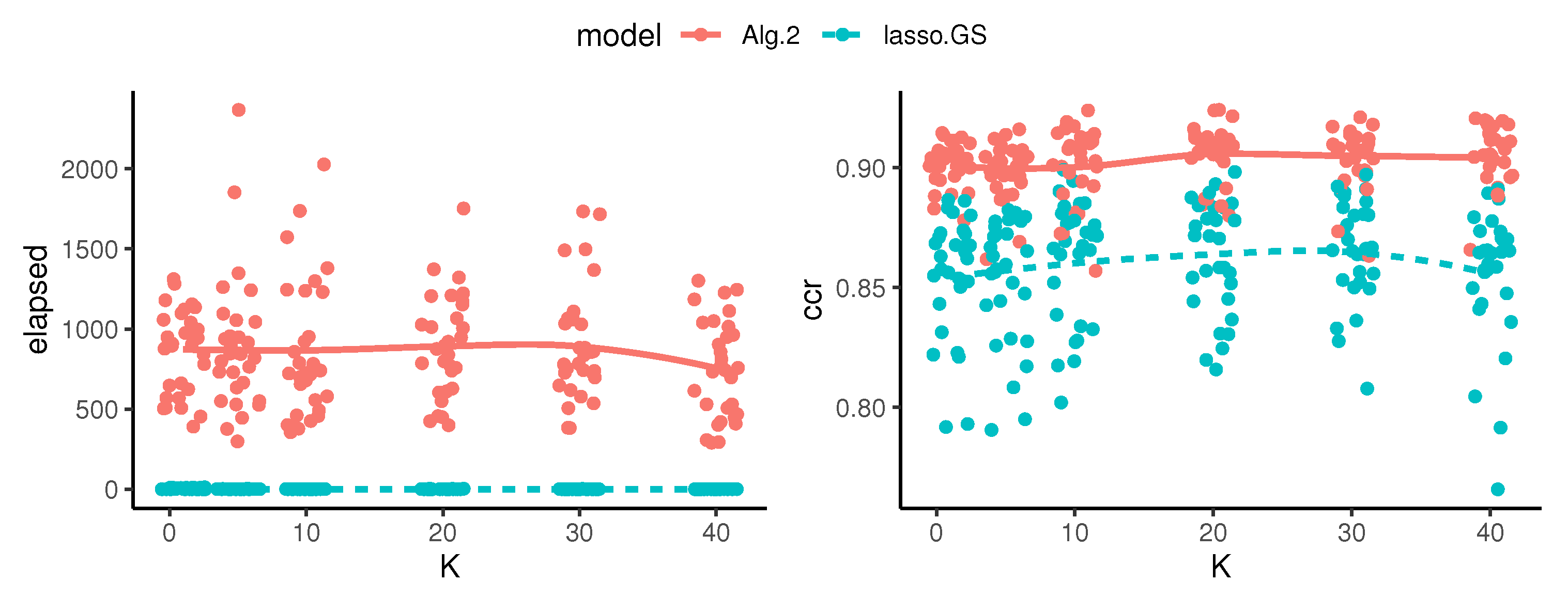
• The iterative sparse group lasso removes the dependence on the hyper-parameters of the sparse group lasso, but is sensible to the train–validate sample partitions. This problem has been solved running the algorithm for a large number of different train–validate sample partitions (Algorithm 2).
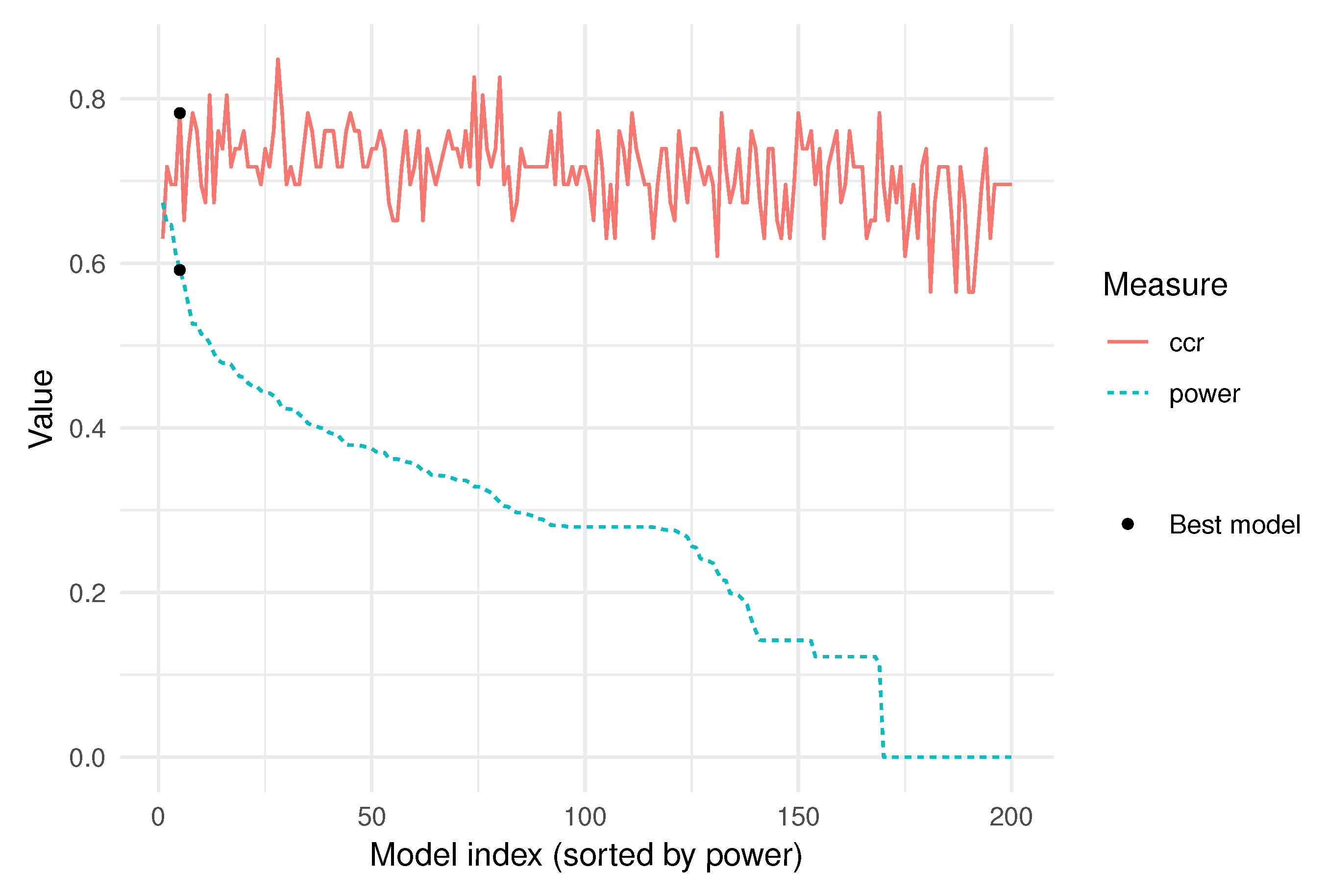
• The correct classification rate of each model in its respective validation sample is stored. Notice that this is an overestimation of the true correct classification rate on future observations, and the highest validation rate does not imply the best model.
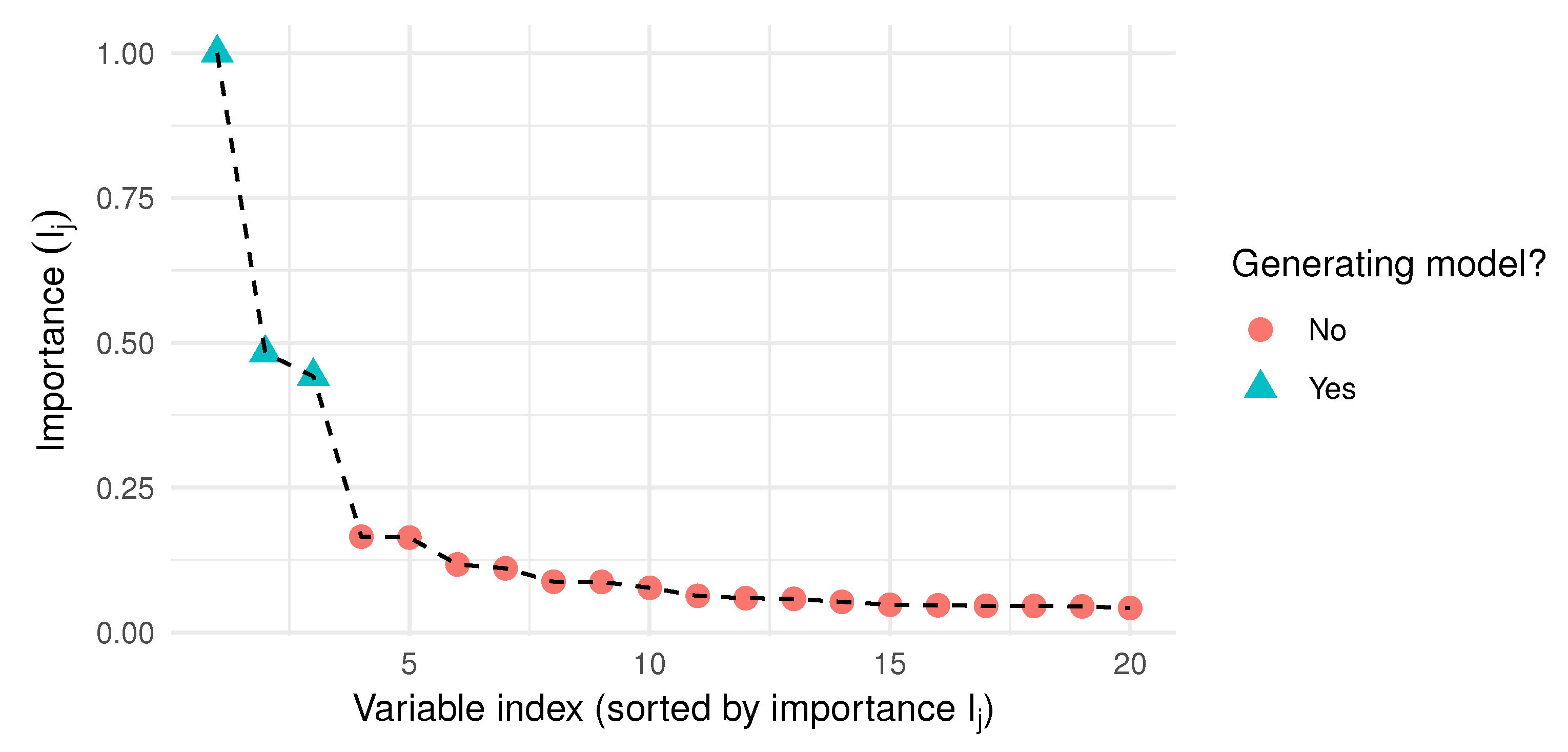
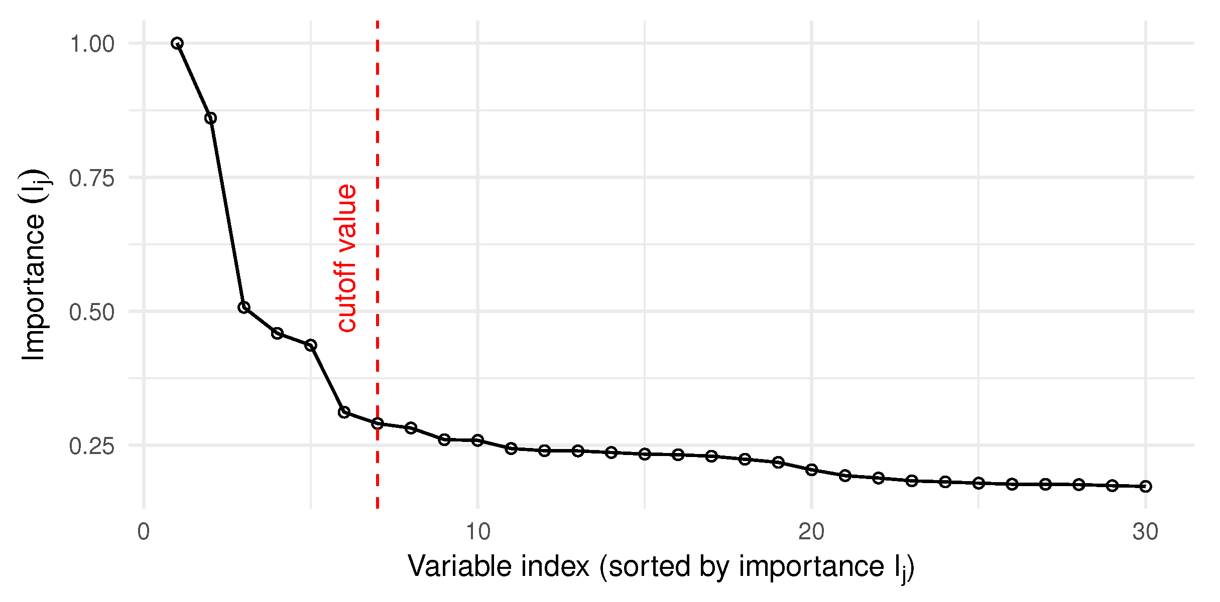
• The importance index weighs the variables, based on the correct classification rate of the models that include them.
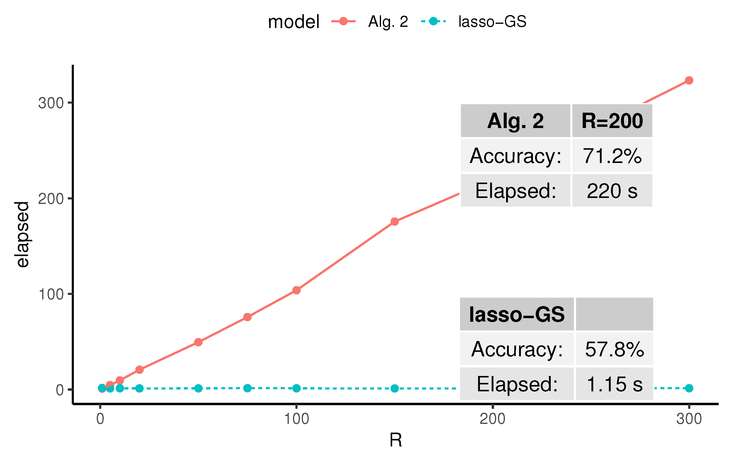
• The power index weighs the models, based on the importance of the variables they include.

This methodology was tested on a sample of TNBC patients, trying to reveal the genetic profile associated with resistance to the treatment of interest. The literature studies mentioned in Section 4 provide a rationale supporting the potential predictive value of the two gene pathways identified in our study (the homeobox-related and the oxidative phosphorylation pathways). In order to validate these results, we are testing the model in a new cohort of TNBC patients from the same clinical trial.

Future studies should examine other strategies to grouping variables, as discussed in Section 2.3, based on supervised algorithms as well as unsupervised ones.

References

1. Ferlay, J.; Soerjomataram, I.; Ervik, M.; Dikshit, R.; Eser, S.; Mathers, C.; Rebelo, M.; Parkin, D.; Forman, D.; Bray, F. GLOBOCAN 2012 v1. 0, Cancer Incidence and Mortality Worldwide: IARC CancerBase No. 11; International Agency for Research on Cancer: Lyon, France, 2013. [Google Scholar]
2. Dent, R.; Trudeau, M.; Pritchard, K.I.; Hanna, W.M.; Kahn, H.K.; Sawka, C.A.; Lickley, L.A.; Rawlinson, E.; Sun, P.; Narod, S.A. Triple-negative breast cancer: clinical features and patterns of recurrence. Clin. Cancer Res. 2007, 13, 4429–4434. [Google Scholar] [CrossRef] [Green Version]
3. Cortazar, P.; Zhang, L.; Untch, M.; Mehta, K.; Costantino, J.P.; Wolmark, N.; Bonnefoi, H.; Cameron, D.; Gianni, L.; Valagussa, P.; et al. Pathological complete response and long-term clinical benefit in breast cancer: the CTNeoBC pooled analysis. Lancet 2014, 384, 164–172. [Google Scholar] [CrossRef] [Green Version]
4. Symmans, W.F.; Wei, C.; Gould, R.; Yu, X.; Zhang, Y.; Liu, M.; Walls, A.; Bousamra, A.; Ramineni, M.; Sinn, B.; et al. Long-Term Prognostic Risk After Neoadjuvant Chemotherapy Associated With Residual Cancer Burden and Breast Cancer Subtype. J. Clin. Oncol. Off. J. Am. Soc. Clin. Oncol. 2017, 35, 1049–1060. [Google Scholar] [CrossRef] [Green Version]
5. Sharma, P.; López-Tarruella, S.; Garcia-Saenz, J.A.; Khan, Q.J.; Gomez, H.; Prat, A.; Moreno, F.; Jerez-Gilarranz, Y.; Barnadas, A.; Picornell, A.C.; et al. Pathological response and survival in triple-negative breast cancer following neoadjuvant carboplatin plus docetaxel. Clin. Cancer Res. 2018, 24, 5820–5829. [Google Scholar] [CrossRef] [Green Version]
6. Tabchy, A.; Valero, V.; Vidaurre, T.; Lluch, A.; Gomez, H.L.; Martin, M.; Qi, Y.; Barajas-Figueroa, L.J.; Souchon, E.A.; Coutant, C.; et al. Evaluation of a 30-gene paclitaxel, fluorouracil, doxorubicin and cyclophosphamide chemotherapy response predictor in a multicenter randomized trial in breast cancer. Clin. Cancer Res. 2010, 16, 5351–5361. [Google Scholar] [CrossRef] [Green Version]
7. Hatzis, C.; Pusztai, L.; Valero, V.; Booser, D.J.; Esserman, L.; Lluch, A.; Vidaurre, T.; Holmes, F.; Souchon, E.; Wang, H.; et al. A genomic predictor of response and survival following taxane-anthracycline chemotherapy for invasive breast cancer. JAMA 2011, 305, 1873–1881. [Google Scholar] [CrossRef] [Green Version]
8. Chang, J.C.; Wooten, E.C.; Tsimelzon, A.; Hilsenbeck, S.G.; Gutierrez, M.C.; Elledge, R.; Mohsin, S.; Osborne, C.K.; Chamness, G.C.; Allred, D.C.; et al. Gene expression profiling for the prediction of therapeutic response to docetaxel in patients with breast cancer. Lancet 2003, 362, 362–369. [Google Scholar] [CrossRef]
9. De Los Campos, G.; Gianola, D.; Allison, D.B. Predicting genetic predisposition in humans: the promise of whole-genome markers. Nat. Rev. Genet. 2010, 11, 880. [Google Scholar] [CrossRef]
10. Lupski, J.R.; Belmont, J.W.; Boerwinkle, E.; Gibbs, R.A. Clan genomics and the complex architecture of human disease. Cell 2011, 147, 32–43. [Google Scholar] [CrossRef] [Green Version]
11. Offit, K. Personalized medicine: New genomics, old lessons. Hum. Genet. 2011, 130, 3–14. [Google Scholar] [CrossRef] [Green Version]
12. Szymczak, S.; Biernacka, J.M.; Cordell, H.J.; González-Recio, O.; König, I.R.; Zhang, H.; Sun, Y.V. Machine learning in genome-wide association studies. Genet. Epidemiol. 2009, 33. [Google Scholar] [CrossRef] [PubMed] [Green Version]
13. Simon, N.; Friedman, J.; Hastie, T.; Tibshirani, R. A sparse-group lasso. J. Comput. Graph. Stat. 2013, 22, 231–245. [Google Scholar] [CrossRef]
14. Tibshirani, R. Regression Shrinkage and Selection via the Lasso. J. R. Stat. Soc. Ser. B (Stat. Methodol.) 1996, 58, 267–288. [Google Scholar] [CrossRef]
15. Yuan, M.; Lin, Y. Model selection and estimation in regression with grouped variables. J. R. Stat. Soc. Ser. B (Stat. Methodol.) 2006, 68, 49–67. [Google Scholar] [CrossRef]
16. Zou, H.; Hastie, T. Regression shrinkage and selection via the elastic net, with applications to microarrays. J. R. Stat. Soc. Ser. B 2003, 67, 301–320. [Google Scholar] [CrossRef] [Green Version]
17. Laria, J.C.; Carmen Aguilera-Morillo, M.; Lillo, R.E. An iterative sparse-group lasso. J. Comput. Graph. Stat. 2019, 28, 722–731. [Google Scholar] [CrossRef]
18. Zou, H.; Hastie, T. Regularization and variable selection via the elastic net. J. R. Stat. Soc. Ser. B (Stat. Methodol.) 2005, 67, 301–320. [Google Scholar] [CrossRef] [Green Version]
19. Azevedo Costa, M.; de Souza Rodrigues, T.; da Costa, A.G.F.; Natowicz, R.; Pádua Braga, A. Sequential selection of variables using short permutation procedures and multiple adjustments: An application to genomic data. Stat. Methods Med Res. 2017, 26, 997–1020. [Google Scholar] [CrossRef]
20. Sharma, P.; López-Tarruella, S.; García-Saenz, J.A.; Ward, C.; Connor, C.; Gómez, H.L.; Prat, A.; Moreno, F.; Jerez-Gilarranz, Y.; Barnadas, A.; et al. Efficacy of neoadjuvant carboplatin plus docetaxel in triple negative breast cancer: Combined analysis of two cohorts. Clin. Cancer Res. 2017, 23, 649–657. [Google Scholar] [CrossRef] [Green Version]
21. Huang, D.W.; Sherman, B.T.; Lempicki, R.A. Systematic and integrative analysis of large gene lists using DAVID bioinformatics resources. Nat. Protoc. 2009, 4, 44–57. [Google Scholar] [CrossRef]
22. Huang, D.W.; Sherman, B.T.; Lempicki, R.A. Bioinformatics enrichment tools: paths toward the comprehensive functional analysis of large gene lists. Nucleic Acids Res. 2008, 37, 1–13. [Google Scholar] [CrossRef] [PubMed] [Green Version]
23. Li, J.; Zhang, Y.; Gao, Y.; Cui, Y.; Liu, H.; Li, M.; Tian, Y. Downregulation of HNF1 homeobox B is associated with drug resistance in ovarian cancer. Oncol. Rep. 2014, 32, 979–988. [Google Scholar] [CrossRef] [PubMed] [Green Version]
24. Hanrahan, K.; O’neill, A.; Prencipe, M.; Bugler, J.; Murphy, L.; Fabre, A.; Puhr, M.; Culig, Z.; Murphy, K.; Watson, R.W. The role of epithelial–mesenchymal transition drivers ZEB1 and ZEB2 in mediating docetaxel-resistant prostate cancer. Mol. Oncol. 2017, 11, 251–265. [Google Scholar] [CrossRef] [PubMed] [Green Version]
25. Marín-Aguilera, M.; Codony-Servat, J.; Reig, Ò.; Lozano, J.J.; Fernández, P.L.; Pereira, M.V.; Jiménez, N.; Donovan, M.; Puig, P.; Mengual, L.; et al. Epithelial-to-mesenchymal transition mediates docetaxel resistance and high risk of relapse in prostate cancer. Mol. Cancer Ther. 2014, 13, 1270–1284. [Google Scholar] [CrossRef] [PubMed] [Green Version]
26. Puhr, M.; Hoefer, J.; Schäfer, G.; Erb, H.H.; Oh, S.J.; Klocker, H.; Heidegger, I.; Neuwirt, H.; Culig, Z. Epithelial-to-mesenchymal transition leads to docetaxel resistance in prostate cancer and is mediated by reduced expression of miR-200c and miR-205. Am. J. Pathol. 2012, 181, 2188–2201. [Google Scholar] [CrossRef] [Green Version]
27. Wishart, D.S.; Feunang, Y.D.; Guo, A.C.; Lo, E.J.; Marcu, A.; Grant, J.R.; Sajed, T.; Johnson, D.; Li, C.; Sayeeda, Z.; et al. DrugBank 5.0: A major update to the DrugBank database for 2018. Nucleic Acids Res. 2017, 46, D1074–D1082. [Google Scholar] [CrossRef]
28. Matassa, D.; Amoroso, M.; Lu, H.; Avolio, R.; Arzeni, D.; Procaccini, C.; Faicchia, D.; Maddalena, F.; Simeon, V.; Agliarulo, I.; et al. Oxidative metabolism drives inflammation-induced platinum resistance in human ovarian cancer. Cell Death Differ. 2016, 23, 1542. [Google Scholar] [CrossRef] [Green Version]
29. Dai, Z.; Yin, J.; He, H.; Li, W.; Hou, C.; Qian, X.; Mao, N.; Pan, L. Mitochondrial comparative proteomics of human ovarian cancer cells and their platinum-resistant sublines. Proteomics 2010, 10, 3789–3799. [Google Scholar] [CrossRef]
30. Chappell, N.P.; Teng, P.n.; Hood, B.L.; Wang, G.; Darcy, K.M.; Hamilton, C.A.; Maxwell, G.L.; Conrads, T.P. Mitochondrial proteomic analysis of cisplatin resistance in ovarian cancer. J. Proteome Res. 2012, 11, 4605–4614. [Google Scholar] [CrossRef]
31. Marrache, S.; Pathak, R.K.; Dhar, S. Detouring of cisplatin to access mitochondrial genome for overcoming resistance. Proc. Natl. Acad. Sci. USA 2014, 111, 10444–10449. [Google Scholar] [CrossRef] [Green Version]
32. Belotte, J.; Fletcher, N.M.; Awonuga, A.O.; Alexis, M.; Abu-Soud, H.M.; Saed, M.G.; Diamond, M.P.; Saed, G.M. The role of oxidative stress in the development of cisplatin resistance in epithelial ovarian cancer. Reprod. Sci. 2014, 21, 503–508. [Google Scholar] [CrossRef] [PubMed] [Green Version]
33. McAdam, E.; Brem, R.; Karran, P. Oxidative Stress–Induced Protein Damage Inhibits DNA Repair and Determines Mutation Risk and Therapeutic Efficacy. Mol. Cancer Res. 2016, 14, 612–622. [Google Scholar] [CrossRef] [PubMed] [Green Version]
Figure 1. Simulated sample from three random variables, that illustrate the grouping based on principal component analysis (PCA).
Mathematics 09 00222 g001
Figure 2. Sorted importance index obtained from Algorithm 2, with R = 150 , and a simulated data sample with N = 100 observations and p = 400 variables.
Mathematics 09 00222 g002
Figure 3. Elapsed time (in seconds) to obtain a solution (left panel) and accuracy (right panel) of Algorithm 2 (Alg. 2) and lasso with grid search (lasso-GS), on 30 independent runs for each K. The simulation design was ZH_d, with n = 100 , p = 1000 , R = 30 , and K varying between 1 and 40. These experiments were run sequentially.
Mathematics 09 00222 g003
Figure 4. Average elapsed time (in seconds) needed to obtain a solution of Algorithm 2 (Alg. 2) and lasso with grid search (lasso-GS), on 30 independent runs for each R. The simulation design was ZH_d, with n = 50 and p = 200 both fixed, and R varying between 1 and 300. These experiments were run sequentially.
Mathematics 09 00222 g004
Figure 5. Sorted Importance indexes, according to the criterion given in (9), and after running Algorithm 2 with R = 200 . The cutoff value was set to K = N / 2 = 7 , as described in Section 2.5.
Mathematics 09 00222 g005
Figure 6. Power index (10), measured in R = 200 models, in decreasing order, with the corresponding correct classification rate (ccr) of each model in the validation sample.
Mathematics 09 00222 g006
Figure 7. Number of included variables in the final model, by groups (top) and total (bottom). Eighteen out of 82 groups were included.
Mathematics 09 00222 g007