Non-Iterative Solution Methods for Cauchy Problems for Laplace and Helmholtz Equation in Annulus Domain

Abstract

This note is concerned with two new methods for the solution of a Cauchy problem. The first method is based on homotopy-perturbation approach which leads to solving a series of well-posed boundary value problems. No regularization is needed in this method. Laplace and Helmholtz equations are considered in an annular region. It is also proved that the homotopy solution for the Laplace operator converges to the actual exact solution. The second method is also non-iterative. It is based on the application of the Green’s second identity which leads to a moment problem for the unknown boundary condition. Tikhonov regularization is used to obtain a stable and close approximation of the missing boundary condition. A number of examples are used to study the applicability of the methods with the presence of noise.

1. Introduction

In this note, we introduce two direct (Non-iterative) methods for the solution of a particular ill-posed elliptic inverse problem. Specific applications of this problem in annulus domains appear in various fields including thermal systems [1], corrosion detection in pipes [2,3], interior boundary evaluation in Tokamak [4,5], reconstruction of interior voltage distribution [6], and continuation of magnetic field [7]. This problem falls within the general area of inverse problems (IHCP) that have numerous applications in various fields of engineering [8,9].

The specific problems studied in this note are the Cauchy problems of elliptic systems such as Laplace and Helmholtz [10,11] operators within annulus domains, where no information on the interior boundary is available.

Due to its importance the literature on this problem is vast. Recent results on this particular problem includes meshless methods [12,13], an optimal regularization method [14], a fitting algorithm [15], singular boundary method [16], discrete Fourier transform method [17], a method based on proper solution space [18], and an energy regularization method [19].

Almost all existing results are iterative [20] (and references therein). Iterative algorithms require an appropriate initial guess, and in case of minimization based algorithms [21], some level of convexity. The purpose of this note is to develop two direct (non-iterative) methods for inverse problems for annular domains. Analytical issues for this problem has been addressed in [22]. Iterative methods for this particular application in fusion research has been developed [4,23] (also references therein). However, fast direct (non-iterative) solution methods are more suitable because they can be used on-line for feedback control. The first method is based on Homotopy-perturbation technique [24].

Homotopy perturbation approach leads to solving a series of well-posed boundary value problems. It does not require any regularization and is direct. In case of partial data, it can also be used as an initial guess for optimization-based iterative methods [25]. It is also proved that this method can recover the exact boundary condition for the Laplace operator. This method is presented in Section 2. We also apply this method to the Helmholtz operator in an annular region which is presented in Section 3. The second method is based on the application of Green’s identity. We have presented a different approach that uses Green’s identity in [26]. Here, we are using point sources to excite the domain, and the formulation is simpler. It also does not require a fictitious domain. This method is also non-iterative and requires regularization. This method is presented in Section 4.

Notation: We use subscripts ${\ast }_x$, ${\ast }_r$, ${\ast }_z$, ${\ast }_{\theta }$ to denote differentiation with respect to the independent variable. We use integer subscript to denote an element in a finite dimensional space. For clarity, we specifically denote the normal derivative at the boundary by $\frac{\partial }{\partial n}$.

2. A Direct Method Based on Homotopy-Perturbation

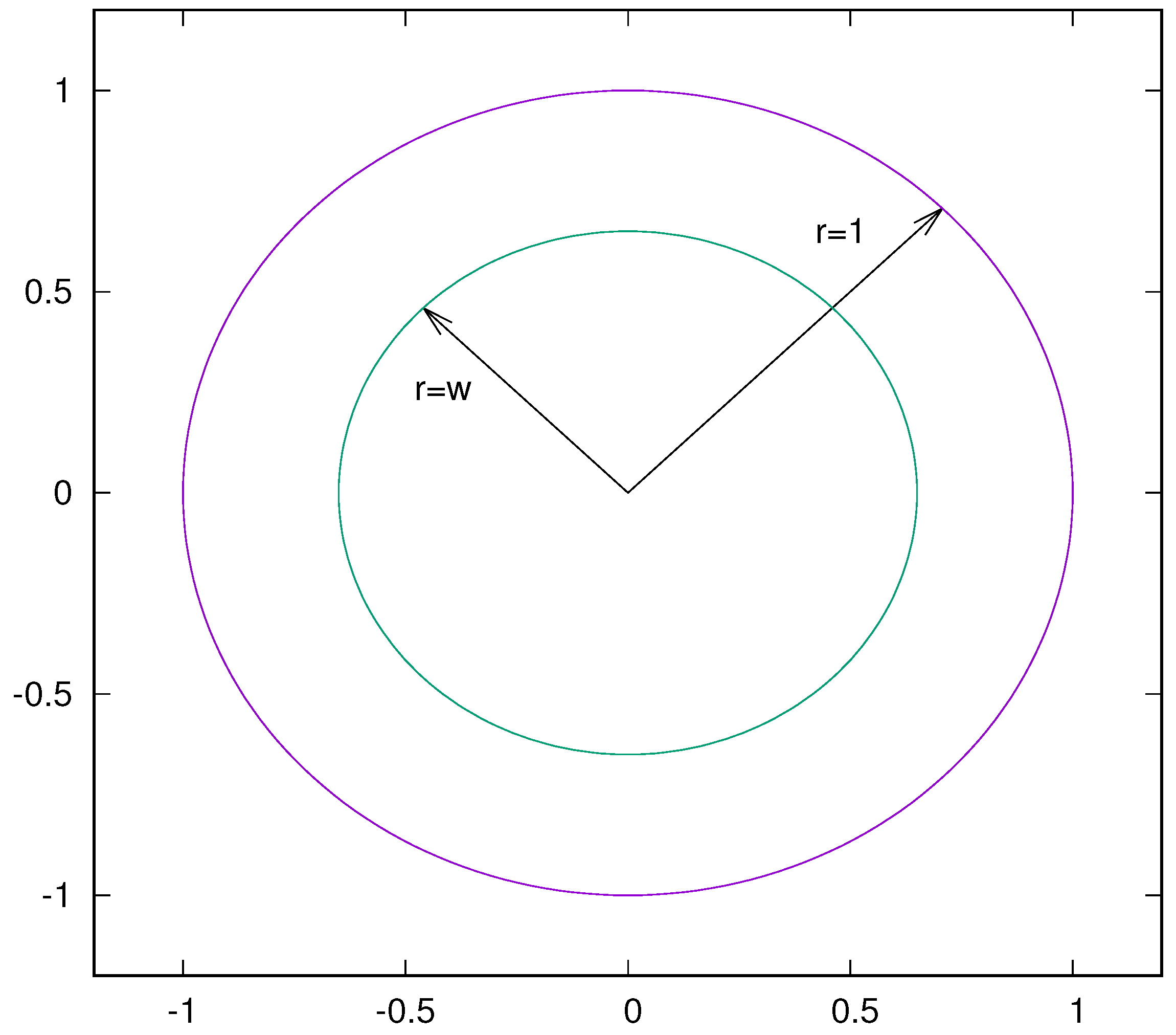
Consider a Cauchy problem for a ring shown in Figure 1, and assume that the outer boundary, i.e., $(r=1)$, is accessible and can be used to collect measurements, and is given by

$$\begin{array}{c}\hfill r^2{u}_{rr}+r{u}_r+u_{\theta \theta }=0,(r,\theta )\in \Omega ,u(1,\theta )=f(\theta ).\end{array}$$

(1)

Measurements in the form of flux can be collected and provided according to

$$\begin{array}{c}\hfill u_r(1,\theta )=g(\theta ).\end{array}$$

(2)

The Cauchy problem of interest is to solve for the temperature $u(r,\theta )$, and in particular the inner boundary condition $u(w,\theta )$. Assuming a homotopy where the scalar $p:0\to 1$, we can consider an elliptic system given by [24]

$$\begin{array}{c}\hfill r^2{u}_{rr}^0+r{u}_r^0-r^2{u}_{rr}-r{u}_r=p\left(r^2{u}_{rr}^0+r{u}_r^0+u_{\theta \theta }\right),(r,\theta )\in \Omega ,\end{array}$$

(3)

where for $p=1$ we recover (1). We can then assume a perturbation for the temperature given by

$$\begin{array}{c}\hfill u(r,\theta )=u^0+p{u}^1+p^2{u}^2+p^3{u}^3+\dots ,\end{array}$$

(4)

where p is the perturbation parameter, and $u^k$ is the temperature at different orders. For various orders it leads to

$$\begin{array}{c}\hfill p^0:r^2{u}_{rr}^0+r{u}_r^0=0,p^1:r^2{u}_{rr}^1+r{u}_r^1=-u_{\theta \theta }^0,p^2:r^2{u}_{rr}^2+r{u}_r^2=-u_{\theta \theta }^1,\dots \end{array}$$

The boundary conditions can also be imposed according to

$$\begin{array}{c}\hfill u^0(1,\theta )=f(\theta ),u_r^0(1,\theta )=g(\theta ),u^k(1,\theta )=u_r^k(1,\theta )=0,,k=1,2,\dots \end{array}$$

(5)

Analytical solutions can be obtained according to

$$\begin{array}{ccc}& & u^0(r,\theta )=g(\theta )ln(r)+f(\theta ),u^1(r,\theta )=-\frac{g^{(2)}}{3!}{\left[ln(r)\right]}^3-\frac{f^{(2)}}{2!}{\left[ln(r)\right]}^2,\hfill \\ & & u^2(r,\theta )=\frac{g^{(4)}}{5!}{\left[ln(r)\right]}^5+\frac{f^{(4)}}{4!}{\left[ln(r)\right]}^4,u^3(r,\theta )=-\frac{g^{(6)}}{7!}{\left[ln(r)\right]}^7-\frac{f^{(6)}}{6!}{\left[ln(r)\right]}^6,\hfill \\ & & u^4(r,\theta )=\frac{g^{(8)}}{9!}{\left[ln(r)\right]}^9+\frac{f^{(8)}}{8!}{\left[ln(r)\right]}^8,\dots \hfill \end{array}$$

where ∗^(ℓ) denotes the ℓ-th order derivative $\frac{d^{\ell }}{d{\theta }^{\ell }}$. For $p=1$, we have the solution given by

$$\begin{array}{ccc}\hfill & & u(r,\theta )=\sum _{k=0}^{\infty }{u}^k(r,\theta )=g(\theta )ln(r)+f(\theta )-\frac{g^{(2)}}{3!}{\left[ln(r)\right]}^3-\frac{f^{(2)}}{2!}{\left[ln(r)\right]}^2\hfill \\ & & +\frac{g^{(4)}}{5!}{\left[ln(r)\right]}^5+\frac{f^{(4)}}{4!}{\left[ln(r)\right]}^4-\frac{g^{(6)}}{7!}{\left[ln(r)\right]}^7-\frac{f^{(6)}}{6!}{\left[ln(r)\right]}^6\hfill \\ & & +\frac{g^{(8)}}{9!}{\left[ln(r)\right]}^9+\frac{f^{(8)}}{8!}{\left[ln(r)\right]}^8+\dots \hfill \end{array}$$

(6)

In a more compact form, it is given by

$$\begin{array}{c}\hfill u(r,\theta )=\sum _{n=0}^{\infty }\frac{{(-1)}^{n+2}{f}^{(2n)}{\left(lnr\right)}^{2n}}{(2n)!}+\sum _{n=0}^{\infty }\frac{{(-1)}^{n+2}{g}^{(2n)}{\left(lnr\right)}^{2n+1}}{(2n+1)!}.\end{array}$$

(7)

Applying the ratio test to the first and second summations leads to

$$\begin{array}{c}\hfill \underset{n\to \infty }{lim}\left|\frac{f^{(2n+2)}{\left(lnr\right)}^2}{f^{(2n)}(2n+1)(2n+2)}\right|,\underset{n\to \infty }{lim}\left|\frac{g^{(2n+2)}{\left(lnr\right)}^2}{g^{(2n)}(2n+2)(2n+3)}\right|,\end{array}$$

(8)

respectively. Therefore, if the functions $f(\theta )$ and $g(\theta )$ are analytic, and if the ratios $g^{(2n+2)}/g^{(2n)}$ and $f^{(2n+2)}/f^{(2n)}$ are bounded for all n, then the two power series converge for all r with $0<w\le r\le 1$. These two conditions are very restrictive, because the functions $g^{(2n)}$, $f^{(2n)}$ can go through zero. Therefore the ratio test can only be used if the functions $f(\theta )$ and $g(\theta )$ and their derivatives satisfy required bounds. The ratio test is sufficient but not necessary. We next proceed to show that $u(r,\theta )$ in Equation (7) is indeed the solution to the elliptic problem posed in Equation (1). The Dirichlet problem for Equation (1) with specified boundary conditions at $r=1$ and $r=w$ is well-posed and has a unique solution [27]. We can proceed as follows. We can use Equation (7) to obtain the missing boundary condition for the problem. Using this condition and the given Dirichlet condition in Equation (1), we can write down the exact solution for the given Dirichlet problem ([27], Section 9.5). Using this solution we can then evaluate the gradient of the temperature at $r=1$, and show that, it is indeed the given gradient condition in Equation (2).

Theorem 1.

(main result) The solution to the Cauchy problem given in Equations (1) and (2) is $u(r,\theta )$ given in Equation (7).

Proof. 

Consider the Dirichlet problem Equation (1) ([27], Section 9.5) for the ring shown in Figure 1. The Dirichlet boundary conditions are given as $u(1,\theta )=f(\theta )$ and $u(w,\theta )=\varphi (\theta )$. We can use the solution obtained in Equation (7) to provide the Dirichlet condition at $r=w$ according to

$$\begin{array}{ccc}\hfill & & u(w,\theta )=\varphi (\theta )=g(\theta )ln(w)+f(\theta )-\frac{g^{(2)}}{3!}{(ln(w))}^3-\frac{f^{(2)}}{2!}{(ln(w))}^2\hfill \\ & & +\frac{g^{(4)}}{5!}{(ln(w))}^5+\frac{f^{(4)}}{4!}{(ln(w))}^4-\frac{g^{(6)}}{7!}{(ln(w))}^7-\frac{f^{(6)}}{6!}{(ln(w))}^6\hfill \\ & & +\frac{g^{(8)}}{9!}{(ln(w))}^9+\frac{f^{(8)}}{8!}{(ln(w))}^8+\dots \hfill \end{array}$$

(9)

The exact solution for this particular Dirichlet problem in given by [27]

$$\begin{array}{ccc}\hfill & & u(r,\theta )=\frac{1}{2}(a_0+b_{0}ln(r))\hfill \\ & & +\sum _{n=1}^{\infty }[(a_n{r}^n+b_n{r}^{-n})cosn\theta +(c_n{r}^n+d_n{r}^{-n})sinn\theta ].\hfill \end{array}$$

(10)

For our specific geometry, the outer radius is $r=1$ and the inner radius is $r=w$, and the coefficients are given by

$$\begin{array}{ccc}& & a_0=\frac{1}{\pi }{\int }_0^{2\pi }f(\tau )d\tau ,b_0=\frac{1}{ln(w)}\left[\frac{1}{\pi }{\int }_0^{2\pi }\varphi (\tau )d\tau -a_0\right],\hfill \\ & & a_n+b_n=\frac{1}{\pi }{\int }_0^{2\pi }f(\tau )cosn\tau d\tau ,w^n{a}_n+w^{-n}{b}_n=\frac{1}{\pi }{\int }_0^{2\pi }\varphi (\tau )cosn\tau d\tau ,\hfill \\ & & c_n+d_n=\frac{1}{\pi }{\int }_0^{2\pi }f(\tau )sinn\tau d\tau ,w^n{c}_n+w^{-n}{d}_n=\frac{1}{\pi }{\int }_0^{2\pi }\varphi (\tau )sinn\tau d\tau ,\hfill \end{array}$$

(11)

We next proceed to use the value of $u(w,\theta )=\varphi (\theta )$ in Equation (9) in Equation (11) and obtain the exact solution for the temperature $u(r,\theta )$ with the Dirichlet conditions $u(1,\theta )=f(\theta )$ and $u(w,\theta )=\varphi (\theta )$. We can then obtain normal derivative $u_r(1,\theta )$ and show that it is indeed the specified $u_r(1,\theta )=g(\theta )$ in Equation (2). Evaluating the gradient $u_r(1,\theta )$ leads to

$$\begin{array}{c}\hfill u_r(r,\theta )=\frac{1}{2}{b}_0+\sum _{n=1}^{\infty }[n(a_n-b_n)cosn\theta +n(c_n-d_n)sinn\theta ],\end{array}$$

(12)

where

$$\begin{array}{ccc}& & b_0=\frac{1}{ln(w)\pi }{\int }_0^{2\pi }(\varphi (\tau )-f(\tau ))d\tau ,\hfill \end{array}$$

(13)

$$\begin{array}{ccc}& & a_n-b_n=\frac{1+w^{2n}}{\pi (1-w^{2n})}{\int }_0^{2\pi }fcosn\tau d\tau -\frac{2w^n}{\pi (1-w^{2n})}{\int }_0^{2\pi }\varphi cosn\tau d\tau ,\hfill \end{array}$$

(14)

$$\begin{array}{ccc}& & c_n-d_n=\frac{1+w^{2n}}{\pi (1-w^{2n})}{\int }_0^{2\pi }fsinn\tau d\tau -\frac{2w^n}{\pi (1-w^{2n})}{\int }_0^{2\pi }\varphi sinn\tau d\tau .\hfill \end{array}$$

(15)

It is easy to note that Equation (12) is the Fourier representation of a function. We can proceed to show that it is indeed the Fourier representation of $g(\theta )$. Considering Equation (11) and substituting for $\varphi (\tau )$ leads to

$$\begin{array}{c}\hfill b_0=\frac{1}{ln(w)\pi }{\int }_0^{2\pi }\left[\left(g(\tau )ln(w)+f(\tau )-\frac{g^{″}}{3!}{(ln(w))}^3-\frac{f^{″}}{2!}(ln{(w)}^2)\dots \right)-f(\tau )\right]d\tau .\end{array}$$

Due to the periodic boundary conditions, the terms involving ${\int }_0^{2\pi }{g}^{(2n)}(\tau )d\tau$ and ${\int }_0^{2\pi }{f}^{(2n)}(\tau )d\tau$ vanish, and the above relation leads to

$$\begin{array}{c}\hfill b_0=\frac{1}{\pi }{\int }_0^{2\pi }g(\tau )d\tau .\end{array}$$

(16)

We next consider Equation (14) and substitute for $\varphi (\theta )$ from Equation (9) which leads to

$$\begin{array}{ccc}& & n(a_n-b_n)=\frac{n(1+w^{2n})}{\pi (1-w^{2n})}{\int }_0^{2\pi }f(\tau )cosn\tau d\tau -\frac{2n{w}^n}{\pi (1-w^{2n})}\hfill \\ & & {\int }_0^{2\pi }\left[\sum _{k=0}^{\infty }\frac{{(-1)}^{k+2}{f}^{(2k)}(\tau ){\left(lnw\right)}^{2k}}{(2k)!}+\sum _{k=0}^{\infty }\frac{{(-1)}^{k+2}{g}^{(2k)}(\tau ){\left(lnw\right)}^{2k+1}}{(2k+1)!}\right]cosn\tau d\tau .\hfill \end{array}$$

Various terms involving ${\int }_0^{2\pi }{g}^{(2n)}(\tau )cosn\tau d\tau$ and ${\int }_0^{2\pi }{f}^{(2n)}(\tau )cosn\tau d\tau$ can be integrated by parts leading to

$$\begin{array}{ccc}& & n(a_n-b_n)=\frac{n(1+w^{2n})}{\pi (1-w^{2n})}{\int }_0^{2\pi }f(\tau )cosn\tau d\tau \hfill \\ & & -\frac{2n{w}^n}{\pi (1-w^{2n})}{\int }_0^{2\pi }\left[1+\frac{{(nln(w))}^2}{2!}+\frac{{(nln(w))}^4}{4!}+\frac{{(nln(w))}^6}{6!}+...\right]f(\tau )cosn\tau d\tau \hfill \\ & & -\frac{2w^n}{\pi (1-w^{2n})}{\int }_0^{2\pi }\left[nln(w)+\frac{{(nln(w))}^3}{3!}+\frac{{(nln(w))}^5}{5!}+...\right]g(\tau )cosn\tau d\tau .\hfill \end{array}$$

(17)

The terms in the second and third integrals on the right hand side converge to

$$\begin{array}{ccc}& & 1+\frac{{(nln(w))}^2}{2!}+\frac{{(nln(w))}^4}{4!}+\frac{{(nln(w))}^6}{6!}...=cosh(nln(w))\hfill \\ & & =\frac{e^{nln(w)}+e^{-nln(w)}}{2}=\frac{w^n+w^{-n}}{2}\hfill \\ & & nln(w)+\frac{{(nln(w))}^3}{3!}+\frac{{(nln(w))}^5}{5!}+...=sinh(nln(w))\hfill \\ & & =\frac{e^{nln(w)}-e^{-nln(w)}}{2}=\frac{w^n-w^{-n}}{2}.\hfill \end{array}$$

Replacing the above terms and simplifying leads to

$$\begin{array}{ccc}& & n(a_n-b_n)={\int }_0^{2\pi }\left[\frac{n(1+w^{2n})}{\pi (1-w^{2n})}-\frac{2n{w}^n}{\pi (1-w^{2n})}\frac{w^n+w^{-n}}{2}\right]f(\tau )cosn\tau d\tau \hfill \\ & & -{\int }_0^{2\pi }\left[\frac{2w^n}{\pi (1-w^{2n})}\frac{w^n-w^{-n}}{2}\right]gcosn\tau d\tau =\frac{1}{\pi }{\int }_0^{2\pi }g(\tau )cosn\tau d\tau .\hfill \end{array}$$

(18)

Following a similar procedure we can show that

$$\begin{array}{c}\hfill n(c_n-d_n)=\frac{1}{\pi }{\int }_0^{2\pi }g(\tau )sinn\tau d\tau .\end{array}$$

(19)

It follows that Equation (12) is indeed the Fourier representation of the gradient of the temperature $u_r(1,\theta )=g(\theta )$. This completes the proof. □

We next consider a numerical example.

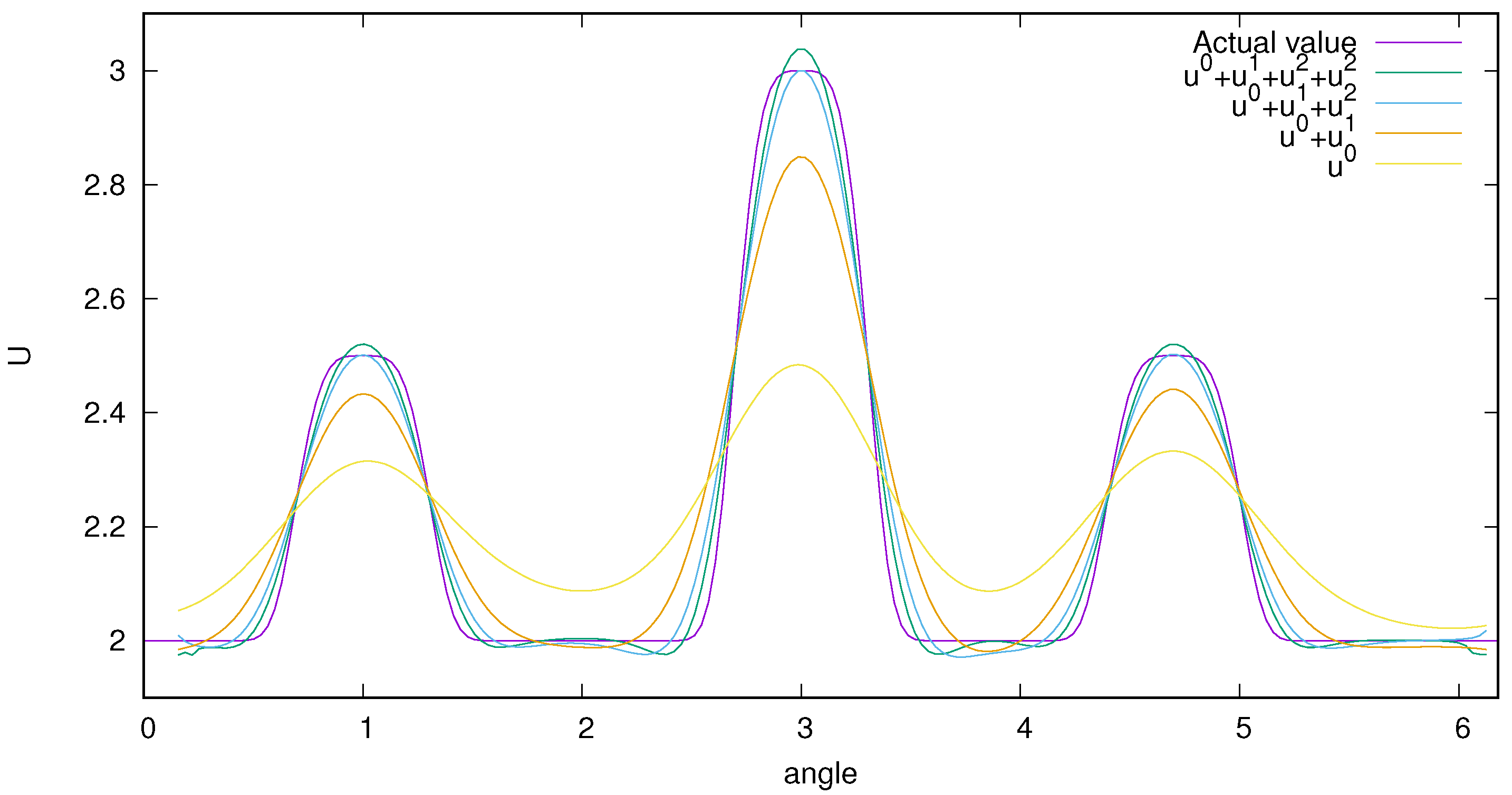
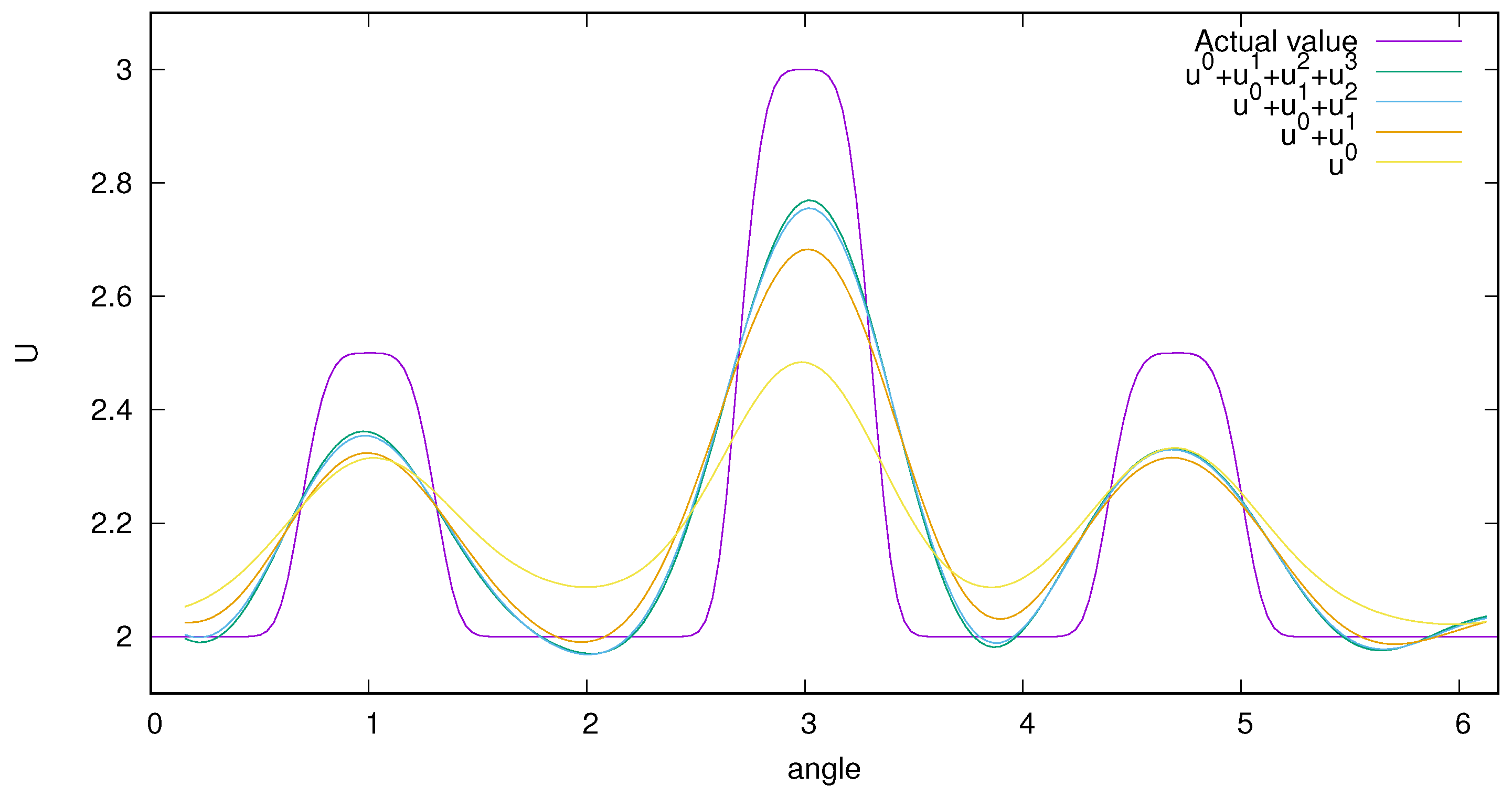
Example 1.

Consider the elliptic system given in Equation (1) and assume that the external boundary condition is given by $u(1,\theta )=f(\theta )=0.5+0.5e^{-{(\theta -\pi )}^2/1.5}$, with the normal gradient at the boundary as the measurement $g(\theta )$. The actual boundary condition is given by

$$\begin{array}{c}\hfill u(w,\theta )=e^{-[{(\theta -1)}^4/0.012]}+2e^{-[{(\theta -3)}^4/0.012]}+e^{-[{(\theta -4.7)}^4/0.012]}.\end{array}$$

We first use this give or actual (or the exact) boundary condition and generate the data, i.e., the gradient at the outer boundary. To simulate a realistic data, we add 3% noise, which is a zero mean, Gaussian, white noise generated with a simple random number generator. We can then provide this as the data. Figure 2 shows the recovered internal boundary at $w=0.63$ with no noise in the data and, Figure 3 presents the results for the same problem with $3\%$ noise.

3. Application to a Helmholtz Equation

Consider a similar Cauchy problem for the Helmholtz equation given by

$$\begin{array}{c}\hfill u_{rr}+\frac{1}{r}{u}_r+\frac{1}{r^2}{u}_{\theta \theta }+k^{2}u=0,(r,\theta )\in \Omega ,u(1,\theta )=f(\theta ),u_r(1,\theta )=g(\theta ),\end{array}$$

(20)

where k is the wave number and, the flux at $r=1$ is provided. Assuming a similar homotopy where the scalar $p:0\to 1$, we can consider an elliptic system given by

$$\begin{array}{c}\hfill u_{rr}^0+\frac{1}{r}{u}_r^0+k^2{u}^0-u_{rr}-\frac{1}{r}{u}_r-k^{2}u=p\left(u_{rr}^0+\frac{1}{r}{u}_r^0+k^2{u}^0+\frac{1}{r^2}{u}_{\theta \theta }\right),\end{array}$$

(21)

where $(r,\theta )\in \Omega$, and for $p=1$ we recover (20). Similarly, the solution can be obtained in the form of a regular perturbation given by

$$\begin{array}{c}\hfill u(r,\theta )=u^0+p{u}^1+p^2{u}^2+p^3{u}^3+\dots ,\end{array}$$

(22)

where various orders of the field variable must satify the following equations

$$\begin{array}{ccc}& & p^0:u_{rr}^0+\frac{1}{r}{u}_r^0+k^2{u}^0=0,p^1:u_{rr}^1+\frac{1}{r}{u}_r^1+k^2{u}^1=-\frac{1}{r^2}{u}_{\theta \theta }^0,\hfill \\ & & p^2:u_{rr}^2+\frac{1}{r}{u}_r^2+k^2{u}^2=-\frac{1}{r^2}{u}_{\theta \theta }^1,\dots \hfill \end{array}$$

(23)

The boundary conditions can also be imposed according to

$$\begin{array}{c}\hfill u^0(1,\theta )=f(\theta ),u_r^0(1,\theta )=g(\theta ),u^k(1,\theta )=u_r^k(1,\theta )=0,,k=1,2,\dots \end{array}$$

(24)

The zero order is the homogenous Bessel equation of order zero. The solution is given by

$$\begin{array}{ccc}\hfill & & u^0(r,\theta )=a_0(\theta )J_0(rk)+b_0(\theta )Y_0(rk),\hfill \\ & & a_0(\theta )=\frac{-1}{d_0(k)}\left(Y_0(k)g(\theta )-\frac{1}{k}{Y}_0^{\prime }(k)f(\theta )\right),\hfill \\ & & b_0(\theta )=\frac{1}{d_0(k)}\left(\frac{1}{k}{J}_0(k)g(\theta )-J_0^{\prime }(k)f(\theta )\right),\hfill \\ & & d_0(k)=J_0(k)Y_0^{\prime }(k)-Y_0(k)J_0^{\prime }(k),\hfill \end{array}$$

(25)

where $J_0(rk)$ and $Y_0(rk)$ are the Bessel functions of order zero. The above solution is unique because the determinant $d_0(k)=\frac{2}{\pi k}$ is away from zero. For $p^1$, we have a nonhomogeous Bessel equation given by

$$\begin{array}{c}\hfill u_{rr}^1+\frac{1}{r}{u}_r^1+k^2{u}^1=-\frac{u_{\theta \theta }^0}{r^2}=\underset{{\Gamma }_0(r,\theta )}{\underbrace{-\frac{1}{r^2}\left(a_0^{″}(\theta )J_0(rk)+b_0^{″}(\theta )Y_0(rk)\right)}},\end{array}$$

(26)

where we are also denoting the known term on the right-hand-side by ${\Gamma }_0(r,\theta )$. The above equation is subject to the boundary condition given in Equation (24). Using the method of variation of parameters [28] (p. 103) the solution is given by

$$\begin{array}{ccc}\hfill & & u^1(r,\theta )=\left[{\int }_{r=w}^1\frac{Y_0(sk){\Gamma }_0(s,k)}{kD(sk)}ds-{\int }_{r=w}^r\frac{Y_0(sk){\Gamma }_0(s,k)}{kD(sk)}ds\right]J_0(rk)\hfill \\ & & +\left[-{\int }_{r=w}^1\frac{J_0(sk){\Gamma }_0(s,k)}{kD(sk)}ds+{\int }_{r=w}^r\frac{J_0(sk){\Gamma }_0(s,k)}{kD(sk)}ds\right]Y_0(rk),\hfill \end{array}$$

(27)

where $D(sk)$ is the Wronskian and is given by $D(rk)=J_0(rk)Y_0^{\prime }(rk)-J_0^{\prime }(rk)Y_0(rk)=\frac{2}{\pi rk}$ for $r\in \Omega$ [29] (p. 302). Since $D(rk)$ is away from zero for $r\in \Omega$, the above solution is well defined. Higher order terms can also be obtained after solving similar nonhomogenous Bessel equations given by

$$\begin{array}{c}\hfill u_{rr}^2+\frac{1}{r}{u}_r^2+k^2{u}^2=-\frac{u_{\theta \theta }^1}{r^2},u_{rr}^3+\frac{1}{r}{u}_r^3+k^2{u}^3=-\frac{u_{\theta \theta }^2}{r^2},\dots \end{array}$$

(28)

We next consider a numerical example for the Helmholtz operator.

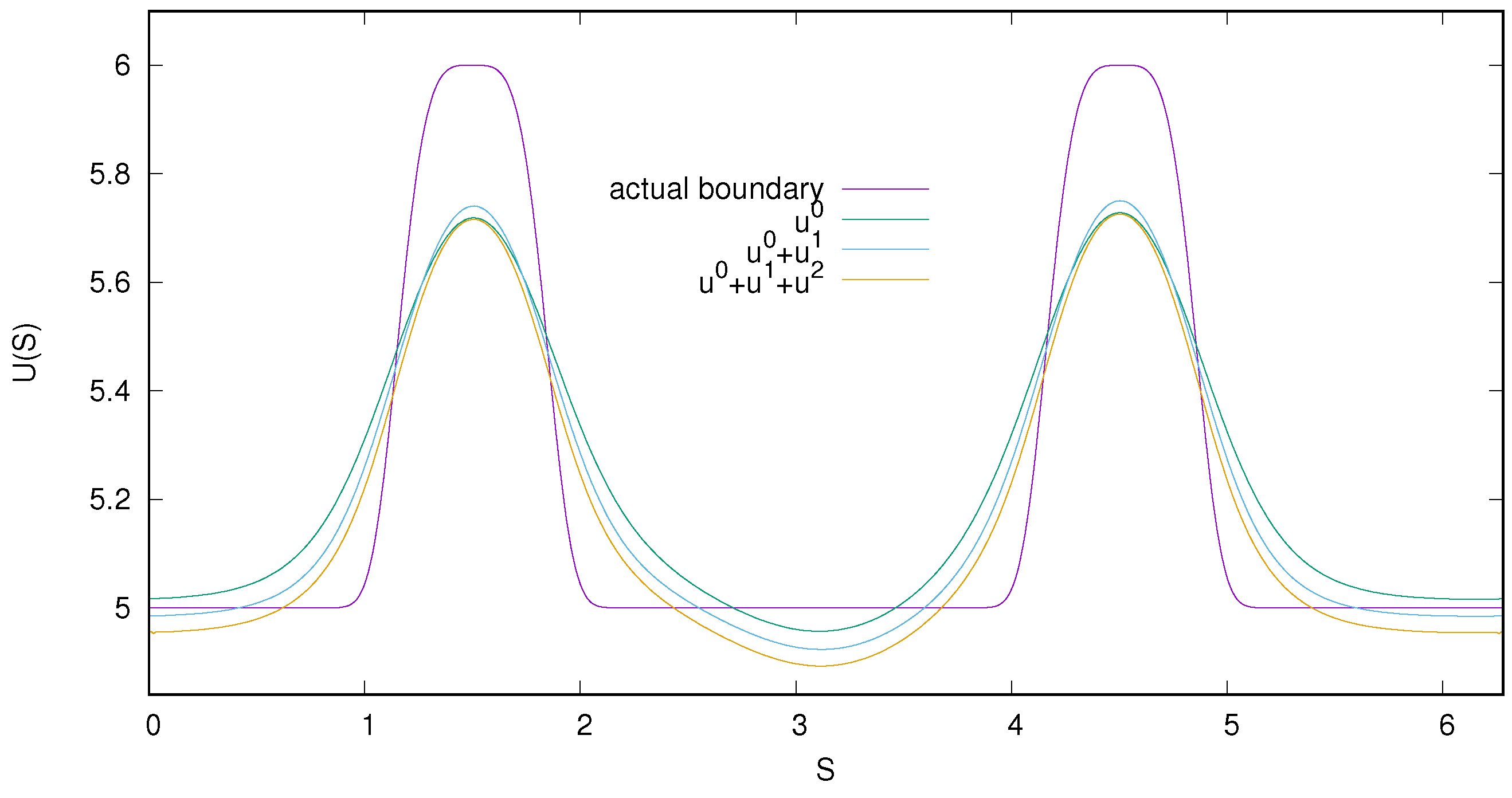
Example 2.

Consider the Cauchy problem for the Helmholtz equation given in Equation (20) and assume that the external boundary condition is given by $u(1,\theta )=f(\theta )=1+0.3e^{{(-(\theta -\pi ))}^2/0.7)}$. The actual boundary condition at $r=w$ is given by

$$\begin{array}{c}\hfill u(w,\theta )=5+e^{(-{(\theta -1.5)}^4/0.02)}+e^{(-{(\theta -4.51)}^4/0.02)},\end{array}$$

(29)

and $k=5$. Figure 4 shows the recovered internal boundary at $w=0.6$. Figure 5 presents the unknown interior boundary for the same boundary condition at $r=1$. The actual interior boundary condition is given by

$$\begin{array}{c}\hfill u(w,\theta )=5+e^{(-{(\theta -1.5)}^4/0.015)}+e^{(-{(\theta -3.51)}^4/0.015)}+1.6e^{(-{(\theta -5.21)}^4/0.015)}.\end{array}$$

(30)

4. A Direct Method in Terms of a Moment Problem

Consider the same bounded domain $\Omega$ shown in Figure 1. The domain is enclosed by smooth boundaries ${\Gamma }_1$ (or $r=1$) and, ${\Gamma }_2$ (or $r=w$) with ${\Gamma }_1\cup {\Gamma }_2=\partial \Omega$ and ${\Gamma }_1\cap {\Gamma }_2=0$. Consider a similar Cauchy problem given by Equation (1), i.e.,

$$\begin{array}{c}\hfill \Delta u(\mathbf{x})=0,\mathbf{x}\in \Omega ,u(\mathbf{x})=f(\theta ),u_n(\mathbf{x})=g(\theta ),\mathbf{x}\in {\Gamma }_1.\end{array}$$

(31)

This is similar to the problem given in (1) and (2), where ${\Gamma }_2$ is the interior boundary where no information is given. Consider two well-posed elliptic problems given by

$$\begin{array}{ccc}& & \Delta \tau (\mathbf{x})=\delta (\mathbf{x}-s_j),\mathbf{x}\in \Omega ,\tau (\mathbf{x})=f(\theta ),\mathbf{x}\in {\Gamma }_1,\tau (\mathbf{x})=0,\mathbf{x}\in {\Gamma }_2,\hfill \end{array}$$

(32)

$$\begin{array}{ccc}& & \Delta \gamma (\mathbf{x})=\delta (\mathbf{x}-s_j),\mathbf{x}\in \Omega ,\gamma (\mathbf{x})={\sigma }_j(\theta ),\mathbf{x}\in {\Gamma }_1,\gamma (\mathbf{x})=0,\mathbf{x}\in {\Gamma }_2,\hfill \end{array}$$

(33)

where $\delta (\mathbf{x}-s_j)$ is a delta function centered at $s_j\in \Omega$, and ${\sigma }_j(\theta )$ is a smooth function chosen by the designer. Applying the Green’s 2-nd identity lead to

$$\begin{array}{c}\hfill {\int }_{\Omega }(u\Delta \tau -\tau \Delta u)d\mathbf{x}={\oint }_{{\Gamma }_1}\left(u\frac{\partial \tau }{\partial n}-\tau \frac{\partial u}{\partial n}\right)ds+{\oint }_{{\Gamma }_2}\left(u\frac{\partial \tau }{\partial n}-\tau \frac{\partial u}{\partial n}\right)ds,\end{array}$$

(34)

$$\begin{array}{c}\hfill {\int }_{\Omega }\left(u\Delta \gamma -\gamma \Delta u\right)d\mathbf{x}={\oint }_{{\Gamma }_1}\left(u\frac{\partial \gamma }{\partial n}-\gamma \frac{\partial u}{\partial n}\right)ds+{\oint }_{{\Gamma }_2}\left(u\frac{\partial \gamma }{\partial n}-\gamma \frac{\partial u}{\partial n}\right)ds,\end{array}$$

(35)

where $\frac{\partial }{\partial n}$ is the outward normal derivative. Using Equations (31)–(33) leads to

$$\begin{array}{ccc}& & {\int }_{\Omega }u\delta (\mathbf{x}-s_j)d\mathbf{x}=u(s_j)={\oint }_{{\Gamma }_1}f\left(\frac{\partial \tau }{\partial n}-g\right)ds+{\oint }_{{\Gamma }_2}u\frac{\partial \tau }{\partial n}ds,\hfill \\ & & {\int }_{\Omega }u\delta (\mathbf{x}-s_j)d\mathbf{x}=u(s_j)={\oint }_{{\Gamma }_1}f\frac{\partial \gamma }{\partial n}ds-{\oint }_{{\Gamma }_1}{\sigma }_{j}gds+{\oint }_{{\Gamma }_2}u\frac{\partial \gamma }{\partial n}ds.\hfill \end{array}$$

(36)

The left hand sides are the field variable at the same point $s_j\in \Omega$. Equating the right hand sides leads to a moment problem given by

$$\begin{array}{c}\hfill {\oint }_{{\Gamma }_2}u(\frac{\partial \tau }{\partial n}-\frac{\partial \gamma }{\partial n})ds={\oint }_{{\Gamma }_1}f(g-\frac{\partial \tau }{\partial n})ds+{\oint }_{{\Gamma }_1}f\frac{\partial \gamma }{\partial n}ds-{\oint }_{{\Gamma }_1}{\sigma }_{j}gds={\lambda }_j,\end{array}$$

(37)

where, the quantities on the right hand side are either known, or can be computed. By changing the location of the delta function $s_j\in \Omega$ and the external sampling function ${\sigma }_j(\theta )$, one can obtain a collection of moment problems for the unknown $u(w,\theta )$ given by

$$\begin{array}{c}\hfill {\oint }_{{\Gamma }_2}u(w,\theta )\left({\left[\frac{\partial \gamma }{\partial n}\right]}_j-{\left[\frac{\partial \tau }{\partial n}\right]}_j\right)ds={\lambda }_j,j=1,2,\dots ,M.\end{array}$$

(38)

The above moment problem can be used to solve for the unknown boundary condition $u(w,\theta )$, if the functions $\left({\left[\frac{\partial \gamma }{\partial n}\right]}_j-{\left[\frac{\partial \tau }{\partial n}\right]}_j\right)$ are linearly independent. Before proceeding to prove the linearly independence of these functions, it is uselful to note that the solution to the elliptic system in Equation (33) (or (32)) is the combination of the solution to two problems, namely,

$$\begin{array}{ccc}& & \Delta {\gamma }_{\delta }(\mathbf{x})=\delta (\mathbf{x}-s_j),\mathbf{x}\in \Omega ,{\gamma }_{\delta }(\mathbf{x})=0,\mathbf{x}\in {\Gamma }_1\cup {\Gamma }_2,\mathrm{and},\hfill \end{array}$$

(39)

$$\begin{array}{ccc}& & \Delta \widehat{\gamma }(\mathbf{x})=0,\mathbf{x}\in \Omega ,\widehat{\gamma }(\mathbf{x})=\sigma (\theta ),\mathbf{x}\in {\Gamma }_1,\widehat{\gamma }(\mathbf{x})=0,\mathbf{x}\in {\Gamma }_2,\hfill \end{array}$$

(40)

where ${\gamma }_{\delta }$ is the solution due to the point source, i.e., Equation (39). Also, $\widehat{\gamma }$ is the solution due to the system being excited at the boundary only, i.e., Equation (40). Since the location of the point source is the same in both problems in Equations (32) and (33), this portion of the solution can be subtracted out. Also, since the boundary condition at ${\Gamma }_1$ is the same, i.e., $f(\theta )$, it is sufficient to state the following theorem.

Theorem 2.

If the functions ${\sigma }_j(\theta )$ and ${\sigma }_k(\theta )$ are linearly independent, then ${\left[\frac{\partial \widehat{\gamma }}{\partial n}\right]}_j$ and ${\left[\frac{\partial \widehat{\gamma }}{\partial n}\right]}_k$ are linearly independent.

Proof. 

It is sufficient to consider two elliptic problems given by

$$\begin{array}{ccc}& & \Delta {\widehat{\gamma }}_j(\mathbf{x})=0,\mathbf{x}\in \Omega ,\widehat{\gamma }(\mathbf{x})={\sigma }_j,\mathbf{x}\in {\Gamma }_1,\widehat{{\gamma }_j}(\mathbf{x})=0,,\mathbf{x}\in {\Gamma }_2,\hfill \end{array}$$

(41)

$$\begin{array}{ccc}& & \Delta {\widehat{\gamma }}_k(\mathbf{x})=0,\mathbf{x}\in \Omega ,\widehat{\gamma }(\mathbf{x})={\sigma }_k,\mathbf{x}\in {\Gamma }_1,\widehat{{\gamma }_k}(\mathbf{x})=0,,\mathbf{x}\in {\Gamma }_2,\hfill \end{array}$$

(42)

The solution to the above problems are given by [27] (pp. 340). Assume that ${\sigma }_j(\theta )$ and ${\sigma }_k(\theta )$ are linearly independent but, ${\left[\frac{\partial \gamma }{\partial n}\right]}_j(\theta )$ and ${\left[\frac{\partial \gamma }{\partial n}\right]}_k(\theta )$ are linearly dependent. If ${\left[\frac{\partial \gamma }{\partial n}\right]}_j(\theta )$ and ${\left[\frac{\partial \gamma }{\partial n}\right]}_k(\theta )$ are linearly dependent, then there must exist a nonzero constand $\mu$ such that ${\left[\frac{\partial \gamma }{\partial n}\right]}_j(\theta )-\mu {\left[\frac{\partial \gamma }{\partial n}\right]}_k(\theta )=0$, $\forall \theta \in [0,2\pi ]$. Solving the elliptic systems for ${\widehat{\gamma }}_k$ and ${\widehat{\gamma }}_j$, computing the normal gradient at $r=w$, multiplying the latter by $\mu$ and subtracting it from the former and simplifying leads to

$$\begin{array}{ccc}\hfill & & {\left[\frac{\partial \widehat{\gamma }}{\partial n}\right]}_j(\theta )-\mu {\left[\frac{\partial \widehat{\gamma }}{\partial n}\right]}_k(\theta )=\frac{-1}{2\pi wln(w)}{\int }_0^{2\pi }({\sigma }_j(\varphi )-\mu {\sigma }_k(\varphi ))d\varphi \hfill \\ \hfill & & +\sum _{\ell =1}^L\left[\frac{2\ell w^{\ell -1}}{\pi (1-w^{2\ell })}{\int }_0^{2\pi }\left[{\sigma }_j(\varphi )-\mu {\sigma }_k(\varphi )\right]cos\ell \varphi d\varphi \right]cos\ell \theta \hfill \\ \hfill & & +\sum _{\ell =1}^L\left[\frac{2\ell w^{\ell -1}}{\pi (1-w^{2\ell })}{\int }_0^{2\pi }\left[{\sigma }_j(\varphi )-\mu {\sigma }_k(\varphi )\right]cos\ell \varphi d\varphi \right]sin\ell \theta =0,\hfill \end{array}$$

(43)

for, ${lim}_{L\to \infty }$. We next argue that if ${\left[\frac{\partial \widehat{\gamma }}{\partial n}\right]}_j(\theta )-\mu {\left[\frac{\partial \widehat{\gamma }}{\partial n}\right]}_k(\theta )=0$ $\forall \theta \in [0,2\pi ]$, then the right-hand-side must be equal to zero for $L=\widehat{L}$, and $L=\widehat{L}+1$, $L=\widehat{L}+2$, $L=\widehat{L}+3$,..., where $\widehat{L}$ is a sufficiently large integer. This leads to ${\sigma }_j(\theta )-\mu {\sigma }_k(\theta )=0$ $\forall \theta \in [0,2\pi ]$, which is a contradiction. This completes the proof. □

The moment problem given in Equation (38) is still ill-posed [30]. Assuming an expansion for the unknown boundary condition $u(w,\theta )$ according to $u(w,\theta )={\sum }_{\ell =1}^L{\xi }_{\ell }{c}_{\ell }(\theta )$, Equation (38) leads to a non-square linear system given by

$$\begin{array}{c}\hfill \underset{\Gamma }{\underbrace{\left[{\oint }_{{\Gamma }_2}{c}_{\ell }{\left[\left(\frac{\partial \gamma }{\partial n}-\frac{\partial \tau }{\partial n}\right)\right]}_{j}ds\right]}}\mathbf{\xi }=\mathbf{\lambda },or,\Gamma \mathbf{\xi }=\mathbf{\lambda },\mathbf{\xi }\in R^L,\mathbf{\lambda }\in R^M,\end{array}$$

(44)

where the unknown coefficients ${\xi }_{\ell }$ are placed in the vector $\mathbf{\xi }$ and the known right-hand side entries ${\lambda }_j$ are placed in the vector $\mathbf{\lambda }$. The above system can be solved after introducing Tikhonov regularization [31] which puts a bound on the slope of the unknown function. We next consider two specific examples.

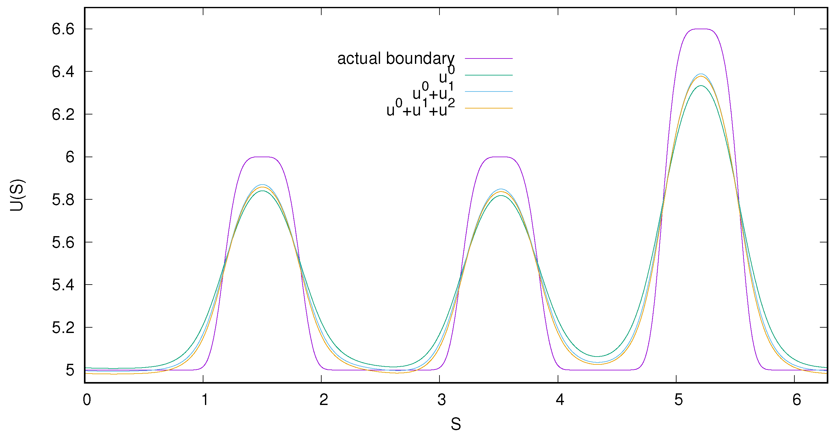
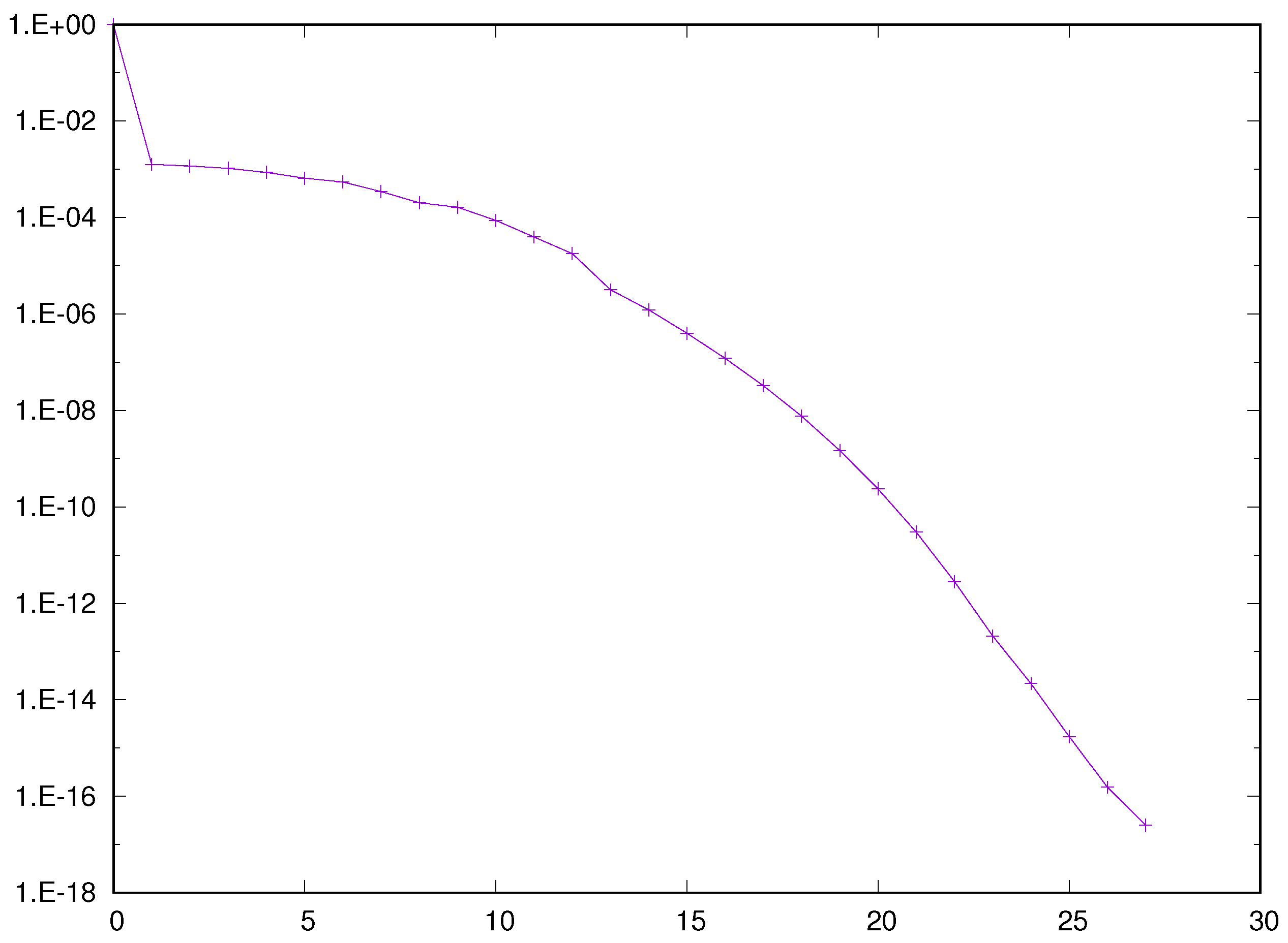
Example 3.

Consider the elliptic system given in Equation (1) and assume that the external boundary condition is given by $f(\theta )=0.5(1+exp(-{(\theta -\pi )}^2/1.5))$. The problem is to recover the temperature at the interior boundary which is located at $w=0.7$. One can choose 30 locations for the point sources, and 30 sampling functions that are denoted by ${\sigma }_j(\theta )$. Dividing the θ direction into 600 equal intervals leads to $d\theta =(2\pi /600)$, and dividing the radial direction into 60 equal intervals leads to $dr=(1-w)/60$. Appropriate locations for the point sources can be given by $s_j=(r_j,{\theta }_j)=((w+(10.5dr)+(7j/6)),((20dt)+j(2\pi /33)))$, for $j=1,2,..,30$. This is to avoid the singularity associated with the solution of Equations in (32) and (33). To generate the sampling functions ${\sigma }_j(\theta ),j=1,2,..,30$ we use a combination of cubic B-splines and sine functions. We essentially need smooth linearly independent functions that satisfy the periodic boundary condition of the problem. We are using Cubic-B splines, and the details are given in [26]. To approximate $u(w,\theta )$ at ${\Gamma }_2$ we use cubic B-splines with $L=28$. Note that L, or the number of unknown coefficients, i.e., ${\xi }_{\ell }$, in the expansion $u(w,\theta )={\sum }_{\ell =1}^L{\xi }_{\ell }{c}_{\ell }(\theta )$ needs to be lower than the number of point sources $M=30$, or $L<M$. Once the location of the point sources and the sampling functions are selected, various terms can be computed and one can proceed to compute the non-square matrix given in (44). Figure 6 shows the normalized singular values of the coefficient matrix Γ. The actual boundary is given by

$$\begin{array}{c}\hfill u(w,\theta )=e^{-[{(\theta -1.3)}^4/0.023]}+1.5e^{-[{(\theta -3)}^4/0.023]}+2e^{-[{(\theta -5)}^4/0.023]}.\end{array}$$

There are about 12 significant (non-zero) eigenvalues out of 28, which is characteristic of a moment problem. In order to be able to invert the matrix, we need to introduce regularization by imposing a bound on the slope of the recovered function. We also need to require that the recovered function be periodic. We can impose that the recovered function be continuous by requiring that

$$\begin{array}{c}\hfill {\xi }_1+4{\xi }_2+{\xi }_3={\xi }_L+4{\xi }_{L-1}+{\xi }_{L-2}.\end{array}$$

(45)

Therefore instead of Equation (44), we proceed to solve a least-square problem given by

$$\begin{array}{c}\hfill \underset{\mathbf{A}}{\underbrace{\left[\begin{array}{c}\Gamma \\ \beta \Phi \\ \alpha \mathbf{\varphi }\end{array}\right]}}\mathbf{\xi }=\underset{\mathbf{b}}{\underbrace{\left[\begin{array}{c}\mathbf{\lambda }\\ 0\\ 0\end{array}\right]}},or,\mathbf{A}\mathbf{\xi }=\mathbf{b},\Rightarrow ,\mathbf{\xi }={[{\mathbf{A}}^T\mathbf{A}]}^{-1}{\mathbf{A}}^T\mathbf{b},\end{array}$$

(46)

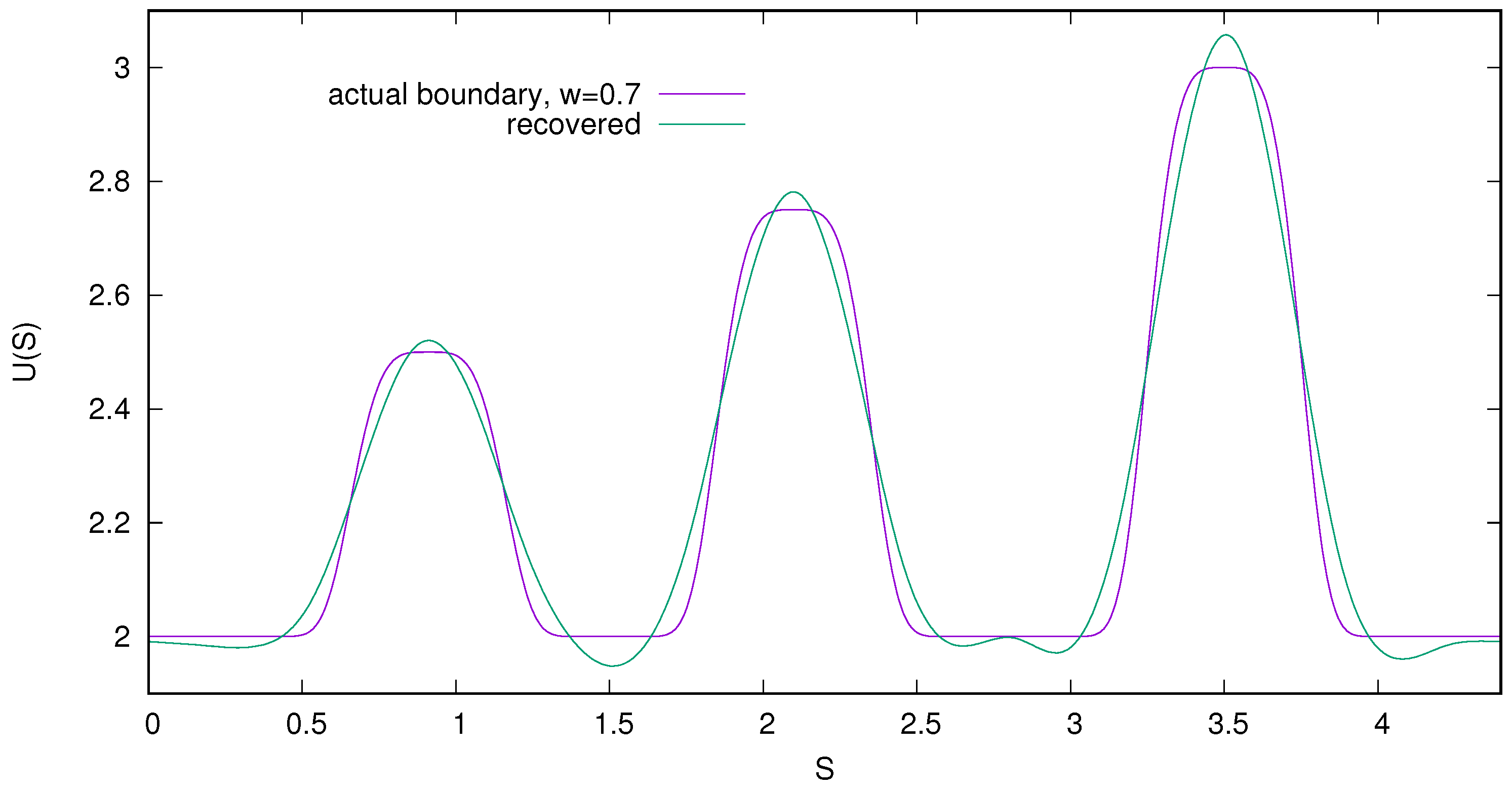
where $\mathsf{\Phi }$ represents the first-derivative operator, and $\mathbf{\varphi }$ represents the condition in (45). For the numerical examples, we use $\beta =0.5\times {10}^{-4}$, and $\alpha =1\times {10}^6$. To ensure a smooth inversion, we use singular-value-decomposition and ignore the singular values lower than $1\times {10}^{-4}$. Figure 7 compares the recovered boundary to the exact value with $0.04\%$ noise level.

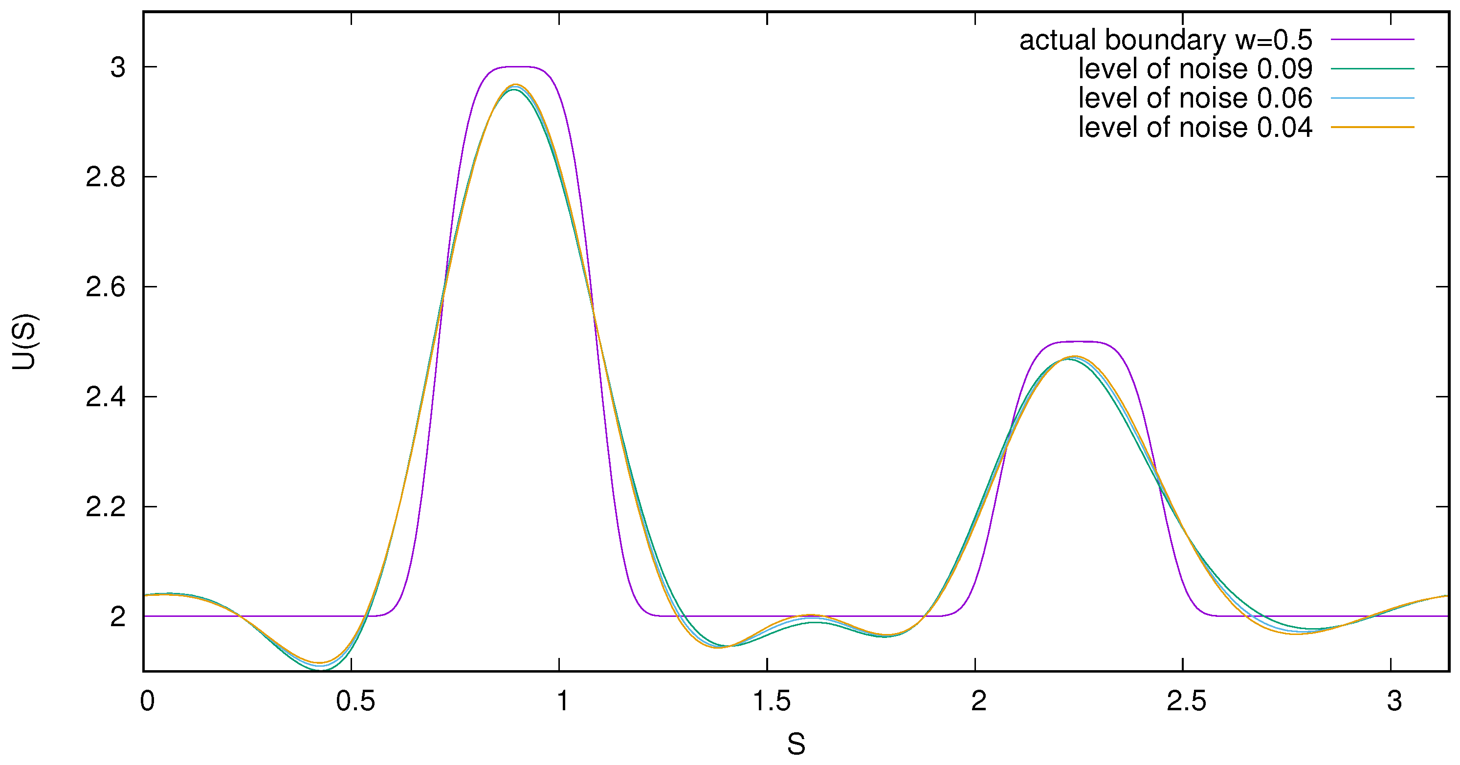
Example 4.

We next consider the same Cauchy problem and study the effect of noise. We also reduce the interior radius to $w=0.5$. We reduce the parameter $\beta =0.1E-4$ and keep the rest of the parameters the same as their values in example 2. The exact value of the boundary condition is given by

$$\begin{array}{c}\hfill u(w,\theta )=2e^{-[{(\theta -1.8)}^4/0.03]}+e^{-[{(\theta -4.5)}^4/0.03]}.\end{array}$$

Figure 8 compares the recovered functions for various levels of noise. The method can recover a very close estimate of the unknown boundary condition directly for various levels of noise. Another feature of both of the methods presented here is that, they both are able to recover a close estimate of unknown boundary conditions where the unknown functions have regions with large gradients.

A number factors can somewhat affect the results. In the work presented here, we did not require for the thickness of the annulus to be small. Methods presented here can recover the unknown boundary condition for all thicknesses. As the interior boundary gets closer to the outer boundary the results improve.

5. Conclusions

In this note we presented two non-iterative (direct) methods for a specific Cauchy problem. The first method is based on Homotopy-perturbation that leads to the solution in the form of a series. We applied this method to Laplace and Helmholtz operators. We also proved that the Homotopy perturbation solution is indeed the unique solusion of the Cauchy prblem for the Laplace operator. The second method is based on the application of the Green’s second identity and leads to a moment problem. Both methods show good robustness to noise. The methods can be applied to a number of elliptic systems.

References

1. Hożejowska, S.; Piasecka, M. Numerical solution of Axisymmetric inverse heat conduction problem by Trefftz method. Energies 2020, 13, 705. [Google Scholar] [CrossRef] [Green Version]
2. Inglese, G. An inverse problem in corrosion detection. Inverse Probl. 1997, 13, 977–994. [Google Scholar] [CrossRef]
3. Choulli, M. An inverse problem in corrosion detection: Stability estimates. J. Inverse Ill Posed Probl. 2004, 12, 349–367. [Google Scholar] [CrossRef]
4. Fischer, Y.; Marteau, B.; Privat, Y. Some inverse problems around the Tokamak Tore Supra. Commun. Pure Appl. Anal. 2012, 11, 2327–2349. [Google Scholar] [CrossRef]
5. Leblond, J.; Mahjoub, M.; Partington, J.R. Analytical extensions and Cauchy-type inverse problems on annular domains: Stability results. J. Inverse Ill Posed Probl. 2006, 14, 189–204. [Google Scholar] [CrossRef]
6. Lee, J.-Y.; Yoon, J.-R. A numerical method for Cauchy problem using singular value decomposition. Commun. Korean Math. Soc. 2001, 16, 478–508. [Google Scholar]
7. Ma, Y.-J.; Fu, C.-L. Cauchy problem for the Laplace equation in cylinder domain. Inverse Probl. Sci. Eng. 2012, 20, 271–285. [Google Scholar] [CrossRef]
8. Hao, D.H.; Dinh, N.H. Methods for Inverse Heat Conduction; Peter Lang Gmbhm Internationaler Verlag Der Wissenschaften: Berlin, Germany, 1998. [Google Scholar]
9. Taler, J.; Duda, P. Solving Direct and Inverse Heat Conduction Problems; Springer: Berlin/Heidelberg, Germany, 2006. [Google Scholar]
10. Marin, L.; Elliot, L.; Heggs, P.J.; Ingham, D.B.; Lesnic, D.; Wen, X. BEM solution for the Cauchy problem associated with Helmholtz-type equations by Landweber method. Eng. Anal. Bound. Elem. 2004, 28, 1025–1034. [Google Scholar] [CrossRef]
11. Shahmurov, R. Solution of the Dirichlet and Neumann problems for a modified Helmholz equation in Bezov spaces on an annulus. J. Differ. Equ. 2010, 249, 526–550. [Google Scholar] [CrossRef] [Green Version]
12. Wu, X.H.; Tao, W.Q. Meshless method based on the local weak-forms for steady-state heat conduction problems. Int. J. Heat Mass Transf. 2008, 51, 3103–3112. [Google Scholar] [CrossRef]
13. Shivanian, E.; Jafarabadi, A. Inverse Cauchy problem of annulus domains in the framework of spectral meshless radial point interpolation. Eng. Comput. 2017, 33, 431–442. [Google Scholar] [CrossRef]
14. He, D.; Pan, K. An order optimal regularization method for the Cauchy problem of a Laplace equation in an annulus domain. Appl. Math. Model. 2015, 39, 3063–3074. [Google Scholar] [CrossRef]
15. Frackowiak, A.; Botkin, N.D.; Cialkowski, M.; Hoffman, K.-H. A fitting algorithm for solving inverse problems of heat conduction. Int. J. Heat Mass Transf. 2010, 53, 2123–2127. [Google Scholar] [CrossRef]
16. Gu, Y.; Chen, W.; He, X.-Q. Singular boundary method for steady-state heat conduction in three dimensional general anisotropic media. Int. J. Heat Mass Transf. 2012, 55, 4837–4848. [Google Scholar] [CrossRef]
17. Wroblewska, A.; Frackowiak, A.; Cialkowski, M. Regularization of the inverse heat conduction problem by the discrete Fourier transform. Inverse Probl. Sci. Eng. 2016, 24, 195–212. [Google Scholar] [CrossRef]
18. Tadi, M. On elliptic inverse heat conduction problems. ASME J. Heat Transf. 2017, 139, 074504. [Google Scholar] [CrossRef]
19. Han, H.; Ling, L.; Takeuchi, T. An energy regularization for Cauchy problems of Laplace equation in Annulus domain. Commun. Comput. Phys. 2011, 9, 878–896. [Google Scholar] [CrossRef]
20. Reinhardt, H.-J.; Hao, D.N.; Frohne, J.; Suttmeier, F.T. Numerical solution of Inverse heat conduction problems in two spatial dimensions. J. Inverse Ill Posed Probl. 2007, 15, 181–198. [Google Scholar] [CrossRef]
21. Wei, T.; Chen, Y.G.; Liu, J.C. A variational-type method of fundamental solutions for the Cauchy problem of Laplace equation. Appl. Math. Model. 2013, 37, 1039–1053. [Google Scholar] [CrossRef]
22. Jaoua, M.; Leblond, J.; Mahjoub, M.; Partington, J.R. Robust numerical algorithms based on analytic approximation for the solution of inverse problems in annular domains. IMA J. Appl. Math. 2009, 74, 481–506. [Google Scholar] [CrossRef] [Green Version]
23. Wang, Y.; Tadi, M. Evaluation of the boundary of the vacuum in a Tokamak. Fusion Eng. Des. 2018, 137, 79–90. [Google Scholar] [CrossRef]
24. Noeiaghdam, S.; Dreglea, A.; He, J.; Avazzadeh, Z.; Suleman, M.; Araghi, M.A.F.; Sidorov, D.N.; Sidorov, N. Error estimation of the Homotopy perturbation method to solve second kind Volterra Integral equations with piecewise smooth Kernels: Application of the CADNA library. Symmetry 2020, 12, 1730. [Google Scholar] [CrossRef]
25. Tadi, M. Evaluation of Elastic Properties in 2-D Non-Homogeneous Solids. Comput. Mech. 2001, 27, 208–218. [Google Scholar] [CrossRef]
26. Tadi, M. A direct method for a Cauchy problem with application to a Tokamak. Theor. Appl. Mech. Lett. 2019, 9, 254–259. [Google Scholar] [CrossRef]
27. Myint-U, T.; Debnath, L. Linear Partial Differential Equations for Scientists and Engineers; Birkhauser: Boston, MA, USA, 2007. [Google Scholar]
28. Myers, G.E. Analytical Methods in Conduction Heat Transfer; Genium: New York, NY, USA, 1987. [Google Scholar]
29. Eom, H.J. Electromagnetic Wave Theory for Boundary Value Problems; Springer: Berlin/Heidelberg, Germany, 2004. [Google Scholar]
30. Ang, D.D.; Gorenflo, R.; Khoi Le, V.; Trong, D.D. Moment Theory and Some Inverse Problems in POTENTIAL Theory and Heat Conduction; Springer: Berlin/Heidelberg, Germany, 2002. [Google Scholar]
31. Tikhonov, A.N.; Arsenin, V.Y. On the Solution of Ill-Posed Problems; John Wiley and Sons: New York, NY, USA, 1977. [Google Scholar]
Figure 1. A cross section of a ring.
Mathematics 09 00268 g001
Figure 2. Recovered unknown interior boundary for the example 1 with no-noise.
Mathematics 09 00268 g002
Figure 3. Recovered unknown interior boundary for the example 1 with 0.03% noise.
Mathematics 09 00268 g003
Figure 4. Recovered unknown interior boundary for example 2, w = 0.6.
Mathematics 09 00268 g004
Figure 5. Recovered unknown interior boundary for example 2, w = 0.7.
Mathematics 09 00268 g005
Figure 6. Significant eigenvalues.
Mathematics 09 00268 g006
Figure 7. Recovered unknown interior boundary for example 3 with (0.04%) noise.
Mathematics 09 00268 g007
Figure 8. Recovered unknown interior boundary for example 4: effect of noise.
Mathematics 09 00268 g008
Publisher’s Note: MDPI stays neutral with regard to jurisdictional claims in published maps and institutional affiliations.