A New Simplified Weak Second-Order Scheme for Solving Stochastic Differential Equations with Jumps

Abstract

In this paper, we propose a new weak second-order numerical scheme for solving stochastic differential equations with jumps. By using trapezoidal rule and the integration-by-parts formula of Malliavin calculus, we theoretically prove that the numerical scheme has second-order convergence rate. To demonstrate the effectiveness and the second-order convergence rate, three numerical experiments are given.

1. Introduction

Many studies are interested in the Lévy process such as the classical stochastic differential equations (SDEs). SDEs have been widely applied to economics and finance [1]. Nowadays, stochastic differential equations with jumps (SDEwJs) are paid more attention by many scholars (see [2,3,4]). As is known, the geometrical and Ornstein–Uhlenbeck (O-U) models are very important in finance, e.g., American option pricing about asset price follows the geometrical model and can be a jump diffusion process (see [4,5]). Chockalingam and Muthuraman [6] studied pricing options when asset prices jump. Li and Zhang [7] employed additive subordination to construct pure jump models for volatility index. Dang, Nguyen and Sewell [8] considered the pricing of Asian options under models that incorporate both regime-switching and jump-diffusions. The O-U process is used to calculate the short term interest rate, and it can also used to account for the mean reversion of prices in modeling commodity processes (see [9]). In this paper, we consider the SDEwJs of the following form:

$$X_t=X_0+{\int }_0^{t}a(s,X_s)ds+{\int }_0^t{\int }_{\mathcal{E}}b(s,e,X_{s-})\tilde{N}(de,ds)$$

(1)

with initial value $X_0\in {\mathbb{R}}^q$. Here, $\mathcal{E}={\mathbb{R}}^q\backslash \{0\}$ is equipped with its Borel field E, $\tilde{N}(de,ds)$ is compensated poisson measure, and the operators $a:[0,t]\times {\mathbb{R}}^q\to {\mathbb{R}}^q$ and $b:[0,t]\times \mathcal{E}\times {\mathbb{R}}^q\to {\mathbb{R}}^q$ are the drift coefficient and the jump coefficient, respectively.

Qualitative theory of the existence and uniqueness of the solution for SDEwJs is studied in [10]. Generally, most of SDEwJs do not have explicit solutions and hence require numerical solutions. It is important to apply appropriate numerical schemes in practice. About numerical solutions of SDEwJs, Platen and Bruti-Liberati [9] systematically introduced the weak schemes and strong schemes with respect to SDEwJs. There are Euler–Maruyama schemes [11], Milstein schemes [12], and jump-adapted schemes [13,14] for solving SDEwJs. Higham and Kloeden [15] presented and analyzed two implicit methods for SDEs and proved in [16] that implicit methods share the same finite time strong convergence rate as the explicit Euler scheme. Hu and Gan [17] studied numerical stability of balanced methods for solving SDEwJs.

Mil’shtein [18] studied the second-order accuracy integration of stochastic differential equations. Similarly, for the higher order numerical methods of SDEwJs, Gardoń [19] proposed the order 1.5 approximation for solutions of jump-diffusion equations. There are [9] the weak or strong order 2.0 Taylor schemes and jump-adapted order 2.0 Taylor schemes. Moreover, the higher order of Runge–Kutta methods for jump-diffusion differential equations can be found in [20]. However, these numerical schemes include multiple stochastic integrals, which are difficult to accurately compute and simulate. Therefore, the simplified weak order 2.0 scheme does not contain the multiple stochastic integrals; particularly, it is convenient and easily calculated for solving SDEwJs in multi-dimensional case. Liu and Li [21] proposed the weak stochastic Taylor order 2.0 (WST2) scheme of SDEwJs with three-point distribution random variables, obtained the convergence rate of the Itô–Taylor scheme, i.e. using the Itô–Taylor expansion and product rule.

In this paper, we propose a new simplified numerical scheme by using the compound Poisson process with a sequence of pairs $({\tau }_k,{\xi }_k)$ of jump time ${\tau }_k$ and marks ${\xi }_k$, where $({\tau }_k,{\xi }_k)$ are uniformly distributed in the square $[0,1]\times [0,1]$. We rigorously prove and obtain its weak second-order convergence rate by using the Malliavin stochastic analysis.

The important contributions of this paper can now be highlighted as follows:

• Our new scheme is simplified without multiple integrals, employs the compound Poisson process with uniformly distribution, and can be easily used to compute the pure jump stochastic models.
• Using a new proof method, i.e. the trapezoidal rule and integration-by-parts formula of Malliavin calculus theory, we rigorously prove that the new scheme has second-order convergence rate.
• We give three experiments to demonstrate the effectiveness and the accuracy of our new scheme, which are consistent with our theoretical results.

Some notations to be used later are listed as follows:

• $C_b^k$ is the set of functions $\psi$:$x\in {\mathbb{R}}^q\to \mathbb{R}$ with uniformly bounded partial derivatives ${\partial }_x^{k_1}\psi$ for $1\le k_1\le k$.
• $C_p^k({\mathbb{R}}^q,\mathbb{R})$ is the set of k times continuously differentiable functions which, together with their partial derivatives of order up to k, have at most polynomial growth.
• C is a generic constant depending only on the upper bounds of derivatives of $a,b$, and g, and it can be different from line to line.

The paper is organized as follows. In Section 2, we introduce some needed preliminaries. In Section 3, we propose a new numerical scheme and obtain its second-order convergence error estimate. In Section 4, three numerical examples are given to verify the theoretical results.

2. Preliminaries

Let there be a filtered probability space $(\Omega ,\mathcal{F},\mathbb{P})$ with the filtration ${\{{\mathcal{F}}_t\}}_{t\ge 0}$, and assume the filtration ${\{{\mathcal{F}}_t\}}_{t\ge 0}$ satisfies the usual hypotheses of completeness, i.e., ${\mathcal{F}}_0$ contains all sets of $\mathbb{P}$-measure zero, and maintains right continuity, i.e., ${\mathcal{F}}_t={\mathcal{F}}_{t+}$. Moreover, the filtration is assumed to be Poisson random measure $N(A,t)$ on $\mathcal{E}\times [0,t]$, where $\mathcal{E}=\mathbb{R}\backslash \{0\}$ is equipped with its Borel field E. Let $\lambda (de)$ be a $\sigma$-finite measure on $(\mathcal{E},E)$ satisfying $\lambda (de):=\gamma (e)de$ with $\gamma (e)\ge 0$ for all $e\in \mathcal{E}$ and $\lambda (de):=0$ for $e\notin \mathcal{E}$, and ${\lambda }_{\mathcal{E}}={\int }_{\mathcal{E}}\gamma (e)de<\infty$. The compensated Poisson random measure can be represented by $\tilde{N}(de,dt)=N(de,dt)-\lambda (de)dt$.

2.1. Itô–Taylor Expansion

Assumption 1.

Assume that the coefficient functions of Equation (1) satisfy the linear growth conditions

$$|a(t,x)|\le C(1+|x|),{\int }_{\mathcal{E}}{|b(t,e,x)|}^2\lambda (de)\le {C(1+|x|}^2).$$

For Equation (1) and $x\in {\mathbb{R}}^q$, we define operators $L^0\phi ,L_e^1\phi$ from $[0,T]\times {\mathbb{R}}^q$ to $\mathbb{R}$

$$\begin{array}{cc}\hfill L^0\phi (t,x)=& \frac{\partial \phi (t,x)}{\partial t}+\sum _{j=1}^q\frac{\partial \phi (t,x)}{\partial x_j}{a}_j(t,x)\hfill \\ & +{\int }_{\mathcal{E}}\left(\phi (t,x+b(t,e,x))-\phi (t,x)-\sum _{j=1}^{q}b(t,e,x)\frac{\partial \phi (t,x)}{\partial x_j}\right)\lambda (de),\hfill \\ \hfill L_e^1\phi (t,x)=& \phi \left(t,x+b(t,e,x)\right)-\phi (t,x),e\in \mathcal{E}.\hfill \end{array}$$

Then, the Itô formula can be presented as:

$$\begin{array}{c}\hfill \phi (t,X_t)=\phi (0,X_0)+{\int }_0^t{L}^0\phi (s,X_s)ds+{\int }_0^t{\int }_{\mathcal{E}}{L}_e^1\phi (s,X_s)\tilde{N}(de,ds).\end{array}$$

(2)

Lemma 1.

(Itô isometry formula) If the stochastic process $\theta (t,e)$ is ${\mathcal{F}}_t$-adapted, then

$$\mathbb{E}\left[{\left({\int }_0^T{\int }_{\mathcal{E}}\theta (t,e)\tilde{N}(de,dt)\right)}^2\right]=\mathbb{E}\left[{\int }_0^T{\int }_{\mathcal{E}}{\theta }^2(t,e)\lambda (de)dt\right].$$

(3)

By Itô–Taylor expansion, we can get a higher order of SDEwJs. However, before we consider the order of approximation, we have to introduce a few additional definitions and notations. We call a row vector $\alpha =(j_1,j_2,\dots ,j_l)$ with $j_i\in \{0,1,\dots ,d\}$ for $i\in \{1,2,\dots ,l\}$ a multi-index of length $l:l(\alpha )\in \{1,2,\dots ,d\}$ and denote by v the multi-index of length zero $(l(v):=0)$. Let $\mathcal{M}$ be the set of all multi-indices, i.e.,

$$\mathcal{M}=\{(j_1,j_2,\dots ,j_l):j_i\in \{0,1,\dots ,d\},i\in \{0,1,\dots ,l\}forl=1,2,\dots \}\cup \{v\}.$$

Assume the hierarchical set

$${\Gamma }_l=\left\{\alpha \in \mathcal{M}:l(\alpha )\le l\right\},$$

and the corresponding remainder set

$$\mathcal{B}({\Gamma }_l)=\left\{\alpha \in \mathcal{M}:l(\alpha )=l+1\right\}.$$

For the time interval $[0,T]$, first we take uniform partitions in temporal domains:

$$0=t_0<···<t_{N-1}<t_N=T$$

with $∆t=t_{n+1}-t_n$ for $n=0,1,\dots ,N-1$. Given a multi-index $\alpha \in \mathcal{M}$ with $l(\alpha )>1$, we write $-\alpha$ and $\alpha -$ for the multi-index in $\mathcal{M}$ by deleting the first and last component of $\alpha$, respectively. Denote by $I_{\alpha }{[g_{\alpha }(·,X_{·})]}_{t_n,t_{n+1}}$ the multiple Itô integral recursively defined by

$$I_{\alpha }{[g_{k,\alpha }(·,X_{·})]}_{t_n,t_{n+1}}=\left\{\begin{array}{c}{\int }_{t_n}^{t_{n+1}}{I}_{\alpha -}{[g_{k,\alpha }(·,X_{·})]}_{t_n,s}ds,l\ge 1,j_l=0,\hfill \\ {\int }_{t_n}^{t_{n+1}}{I}_{\alpha -}{[g_{k,\alpha }(·,X_{·})]}_{t_n,s_l}d{\tilde{N}}_{s_l},l\ge 1,j_l=1,\hfill \end{array}\right.$$

(4)

where the Itô coefficient functions $g_{k,\alpha }$ are defined by

$$g_{k,\alpha }=\left\{\begin{array}{c}{g}_{k,(0)}=a_k,g_{k,(i)}=b_k,l=1.\hfill \\ L_e^1{b}_{k,-\alpha },l>1.\hfill \end{array}\right.$$

(5)

For $\alpha =(1,1,1)$, we define

$$I_{(0,0,0)}^{{\lambda }_{\alpha }}{[H(·,X_{.})]}_{t_n,t_{n+1}}={\int }_{t_n}^{t_{n+1}}{\int }_{\mathcal{E}}{\int }_{t_n}^{s_3}{\int }_{\mathcal{E}}{\int }_{t_n}^{s_2}{\int }_{\mathcal{E}}H(s_1,X_{s_1})\lambda (de)d{s}_1\lambda (de)d{s}_2\lambda (de)d{s}_3.$$

Then, we have the Itô–Taylor expansion

$$\begin{array}{c}\hfill X_{k,t_{n+1}}^n=X_k^n+\sum _{\alpha \in {\Gamma }_2\backslash \{v\}}{g}_{k,\alpha }(t_n,X^n)I_{\alpha }{[1]}_{t_n,t_{n+1}}+\sum _{\alpha \in \mathcal{B}({\Gamma }_2)}{I}_{\alpha }{[g_{k,\alpha }(·,X_{·}^n)]}_{t_n,t_{n+1}}.\end{array}$$

(6)

2.2. The Weak Schemes for Solving SDEwJs

The simple numerical method for the approximate solution of the SDEwJs is the Euler scheme. Thus, we introduce the Euler scheme for solving SDEwJs. Thanks to Itô–Taylor expansion, we can obtain weak convergence schemes for solving SDEsJs as follows.

Scheme 1.

(Euler Scheme) (See [9]) Assume the initial condition$X_0$. For$0\le n\le N-1$, we have

$$\begin{array}{c}\hfill X^{n+1}=X^n+a(t_n,X^n)∆t+b(t_n,X^n)∆{\tilde{N}}_n\end{array}$$

(7)

where$∆{\tilde{N}}_n={\tilde{N}}_{t_{n+1}}-{\tilde{N}}_{t_n}$and$∆t=t_{n+1}-t_n$.

When accuracy and efficiency are required, it is important to construct numerical methods with higher order of convergence. With respect to weak second-order scheme, Liu and Li [21] proposed the weak stochastic Taylor (WST2) scheme and approximated the Poisson jump measure by using three point distribution.

Scheme 2.

(WST2 Scheme) Assume the initial condition$X_0$. For$0\le n\le N-1$, we have

$$\begin{array}{cc}\hfill X^{n+1}=& X^n+a(t_n,X^n)∆t+\sum _{k=1}^{T_n}b(t_n,e_{nk},X^n)+\frac{1}{2}{\tilde{L}}^{0}a(t_n,X^n){(∆t)}^2\hfill \\ \hfill & +\frac{1}{2}\sum _{k=1}^{T_n}\left(L_e^{1}a(t_n,X^n)+{\tilde{L}}^{0}b(t_n,e_{nk},X^n)\right)∆t+\frac{1}{2}{L}_e^{1}b(t_n,e_{nk},X^n)(T_n^2-T_n),\hfill \end{array}$$

(8)

where${\tilde{L}}^0=\frac{\partial }{\partial t}+\sum _{j=1}^q{a}_j(t,x)\frac{\partial }{\partial x_j}$, $\{e_{nk}\}$are independently distributed in a measurable space$\mathcal{E}$with geometric probability law$\frac{\lambda (de)}{{\lambda }_{\mathcal{E}}}$and$T_n$obeys three-point distribution, which has the following probability law:

$$\begin{array}{c}\hfill \mathbb{P}\{T_n=0\}=1-{\lambda }_{\mathcal{E}}∆t+\frac{1}{2}{({\lambda }_{\mathcal{E}}∆t)}^2,\mathbb{P}\{T_n=1\}={\lambda }_{\mathcal{E}}∆t-{({\lambda }_{\mathcal{E}}∆t)}^2,\mathbb{P}\{T_n=2\}=\frac{1}{2}{({\lambda }_{\mathcal{E}}∆t)}^2.\end{array}$$

Then, Buckwar and G. Riedler [20] proposed the Runge–Kutta second-order implicit scheme for solving SDEwJs.

Scheme 3.

(Runge–Kutta Scheme) Assume the initial condition$X_0$. For$0\le n\le N-1$, we have

$$\begin{array}{c}\hfill X^{n+1}=X^n+\frac{1}{2}a\left(t_n,S_1^n\right)∆t+\frac{1}{2}a\left(t_{n+1},S_2^n\right)∆t+b(t_n,X^n)∆{\tilde{N}}_n,\end{array}$$

(9)

$$\begin{array}{c}\hfill S_1^n=X^n,S_2^n=X^n+\frac{1}{2}a\left(t_n,S_1^n\right)∆t+\frac{1}{2}a\left(t_{n+1},S_2^n\right)∆t,\end{array}$$

(10)

where$∆{\tilde{N}}_n={\tilde{N}}_{t_{n+1}}-{\tilde{N}}_{t_n}$and$∆t=t_{n+1}-t_n$.

In addition, the discrete-time approximations considered are divided into regular and jump-adapted schemes. Regular schemes employ time discretizations that do not include the jump times of the Poisson jump measure and Jump-adapted time discretizations include these jump times. Platen and Bruti-Liberati [9] proposed the following jump-adapted weak second-order scheme.

Scheme 4.

(Jump-adapted weak 2-order Scheme) Assume the initial condition$X_0$. For$0\le n\le M-1$, we consider a jump-adapted time discretization$0=t_0<t_1<···<t_M=T$, which is constructed by a superposition of jump times$\{{\tau }_1,{\tau }_2,···\}$of the compensated Poisson measure$\tilde{N}(de,dt)$and equidistant time discretization with step size$∆t$, as given in Section 2.1. For convenience, we set$X_{t_n}=X^n$in this section and define

$$X_{-}^{n+1}=\underset{s\uparrow t_{n+1}}{lim}{X}_s,$$

in the almost sure limit. We have the weak second-order scheme

$$X^{n+1}=X_{-}^{n+1}+b(t_n,X_{-}^{n+1})∆{\tilde{N}}_n$$

(11)

with

$$X_{-}^{n+1}=X^n+a(t_n,X^n)∆t+\frac{1}{2}{L}^{0}a(t_n,X^n){(∆t)}^2,$$

(12)

where$∆{\tilde{N}}_n={\tilde{N}}_{t_{n+1}}-{\tilde{N}}_{t_n}$and$∆t=t_{n+1}-t_n$$(0\le n\le M-1)$.

Remark 1.

Comparing the above methods to solve SDEwJs, the coefficients of Runge–Kutta implicit scheme for solving SDEwJs are not easily determined; the WST2 scheme in [21] needs to consider the probability law of three point distribution and Poisson jump marks, and Jump-adapted weak second-order scheme needs to consider time discretizations that include these jump times.

2.3. Malliavin Stochastic Calculus

Suppose that H is a real separable Hilbert space with scalar product denoted by ${⟨·,·⟩}_H$. The norm of an element $h\in H$ is denoted by ${\parallel h\parallel }_H$. Let the operator $D^k$ be the Malliavin derivative of order k with respect to the lévy process. A random variable F is Malliavin differentiable if and only if $F\in {\mathbb{D}}_{1,2}$, where the space ${\mathbb{D}}_{1,2}\subset L^2(\mathbb{P})$ is defined by completion with respect to the norm ${\parallel ·\parallel }_{1,2}$. The Malliavin derivative of Poisson process (see [22] for details) has the following definition:

$$D_{s_1\dots s_l,e}^{\alpha }=D_{s_1\dots s_l,e}^{(j_1,\dots ,j_l)}=D_{s_1,e}^{j_1}···D_{s_l,e}^{j_t}$$

with especially $D_{s_i,e}^0=1$ for $1\le i\le l$.

Lemma 2.

Let $F\in {\mathbb{D}}_{1,2}$ and $\theta (t,e)\in {\mathbb{D}}_{1,2}$ for $0\le t\le T$. Then, we have the duality formula

$$\begin{array}{cc}\hfill & \mathbb{E}\left[F{\int }_0^T{\int }_{\mathcal{E}}\theta (t,e)\tilde{N}(de,dt)\right]=\mathbb{E}\left[{\int }_0^T{\int }_{\mathcal{E}}\theta (t,e)D_{t,e}F\lambda (de)dt\right],and\hfill \\ \hfill & D_{t,e}{\int }_0^T\theta (s,e)d{\tilde{N}}_s=\theta (t,e)+{\int }_t^T{D}_{t,e}\theta (s,e)d{\tilde{N}}_s.\hfill \end{array}$$

Example 1.

Choose $F={\int }_0^T{\int }_{\mathcal{E}}f(t,e)\tilde{N}(de,dt)$, with the deterministic integral $f\in L^2(\tilde{N}\times \lambda )$. Then, $F=I_1(f)$ and hence

$$D_{t,e}F=f(t,e).$$

In particular, if $F=\eta (T):={\int }_0^T{\int }_{\mathcal{E}}e\tilde{N}(de,dt)$, then

$$D_{t,e}\eta (T)=e.$$

Lemma 3.

(Chain rule) Let $F,G\in {\mathbb{D}}_{1,2}$, then $FG\in {\mathbb{D}}_{1,2}$ and

$$D_{t,e}(FG)=F{D}_{t,e}G+G{D}_{t,e}F+D_{t,e}F{D}_{t,e}G.$$

By induction, it follows that, if $F\in {\mathbb{D}}_{1,2}$, then

$$D_{t,e}(F^n)={(F+D_{t,e}F)}^n-F^n.$$

Let $F\in {\mathbb{D}}_{1,2}$ and φ be a real continuous function on $\mathcal{E}$. Suppose $\phi (F)\in L^2(P)$ and $\phi (F+D_{t,e}F)\in L^2(\mathbb{P}\times \tilde{N}\times \lambda )$. Then, $\phi (F)\in {\mathbb{D}}_{1,2}$ and

$$D_{t,e}\phi (F)=\phi (F+D_{t,e}F)-\phi (F).$$

(13)

Example 2.

Assume $∆{\tilde{N}}_n^{}={\int }_{t_n}^{t_{n+1}}{\int }_{\mathcal{E}}\tilde{N}(de,dt)={\tilde{N}}_{t_{n+1}}^{}-{\tilde{N}}_{t_n}^{}$. Using Itô formula on ${({\tilde{N}}_t-{\tilde{N}}_{t_n})}^2$ yields

$${\int }_{t_n}^{t_{n+1}}{\int }_{t_n}^{t}d{\tilde{N}}_{s}d{\tilde{N}}_t=\frac{1}{2}\left({(∆{\tilde{N}}_n)}^2-{\lambda }_{\mathcal{E}}∆t-∆{\tilde{N}}_n\right).$$

According to Lemma 3, by chain rule (13), taking Malliavin derivatives with respect to $∆{\tilde{N}}_n$ and ${(∆{\tilde{N}}_n)}^2$, we obtain

$$D_{t,e}∆{\tilde{N}}_n=1,D_{t,e}{(∆{\tilde{N}}_n)}^2=2∆{\tilde{N}}_n+1,D_{t,e}{D}_{s,e}{(∆{\tilde{N}}_n)}^2=2,D_{s,e}{\int }_{t_n}^{t_{n+1}}{\int }_{t_n}^{t}dsd{\tilde{N}}_t=s-t_n.$$

3. Main Results

For simple representation, we assume $X_{k,t_{n+1}}^n:=X_{k,t_{n+1}}^{t_n,X^n},$ which is the kth component of $X_{t_{n+1}}^{t_n,X^n}$. It follows from Itô–Taylor formula and trapezoidal rule that

$$\begin{array}{cc}\hfill X_{k,t_{n+1}}^n=& X_k^n+{\int }_{t_n}^{t_{n+1}}{a}_k(s,X_s^n)ds+{\int }_{t_n}^{t_{n+1}}{\int }_{\mathcal{E}}{b}_k(s,X_s^n)\tilde{N}(de,ds)=X_k^{n+1}+R_k^{n+1},\hfill \end{array}$$

(14)

where

$$\begin{array}{cc}\hfill R_k^{n+1}=& L_e^1{a}_k\left[{\int }_{t_n}^{t_{n+1}}{\int }_{t_n}^{t}d{\tilde{N}}_s^{}dt-\frac{1}{2}∆{\tilde{N}}_n^{}∆t\right]\hfill \\ & +L^0{b}_k\left[{\int }_{t_n}^{t_{n+1}}{\int }_{t_n}^{t}dsd{\tilde{N}}_t-\frac{1}{2}∆t∆{\tilde{N}}_n\right]+\sum _{\alpha \in \mathcal{B}({\Gamma }_2)}{I}_{\alpha }{[g_{k,\alpha }(·,X_{·}^n)]}_{t_n,t_{n+1}}.\hfill \end{array}$$

(15)

Here, we write $a_k$ for $a_k(t_n,X^n)$ and $b_k$ for $b_k(t_n,X^n)$. Then, we have the following scheme.

Scheme 5.

Assume the initial condition$X_0$. For$0\le n\le N-1$, we solve$X^{n+1}$with its kth component$X_k^{n+1}$by

$$\begin{array}{cc}\hfill X_k^{n+1}=& X_k^n+a_k∆t+b_k∆{\tilde{N}}_n+\frac{1}{2}{L}^0{a}_k{(∆t)}^2+\frac{1}{2}\left(L_e^1{a}_k+L^0{b}_k\right)∆t∆{\tilde{N}}_n\hfill \\ \hfill & +\frac{1}{2}{L}_e^1{b}_k({(∆{\tilde{N}}_n)}^2-{\lambda }_{\mathcal{E}}∆t-∆{\tilde{N}}_n),\hfill \end{array}$$

(16)

where$∆{\tilde{N}}_n={\tilde{N}}_{t_{n+1}}-{\tilde{N}}_{t_n}$and$∆t=t_{n+1}-t_n$.

Remark 2.

Unlike jump-adapted scheme, Scheme 5 employs regular time discretization, and it is a simplified scheme, which does not involve multiple stochastic integrals. If the jump coefficient function $b=b(t,X_t,e)$, we generate the compound Poisson process

$${\int }_{t_n}^{t_{n+1}}{\int }_{\mathcal{E}}b(s,X^n,e)N(de,ds)=\sum _{k=N_{t_n}+1}^{N_{t_{n+1}}}b({\tau }_k,X^n,{\xi }_k)$$

for simulating compensated Poisson process, where the pairs $({\tau }_k,{\xi }_k)$ are uniformly distributed in the square $[0,1]\times [0,1]$. We found that Scheme 5 has a little impact of the random generation of the compound Poisson process in Example 3. From the numerical experiments, comparing with the three point distribution in WST2 Scheme in [17], our scheme can be implemented in programming and costs less run time. Scheme 5 is an explicit scheme different from Runge–Kutta implicit scheme in [20]. Moreover, in the next subsection, using the integration-by-parts formula of Malliavin calculus, we theoretically prove that our scheme has second-order convergence rate.

Local Weak Convergence Theorem

In this section, using Malliavin stochastic analysis and Itô–Taylor expansion, we obtain the local weak order-2.0 convergence of our new weak second-order scheme.

Theorem 1.

(Local weak convergence) Suppose $X_{t_{n+1}}^n$ and $X^{n+1}$ $(0\le n\le N-1)$ satisfy Equation (1) and Scheme 5, respectively. Under Assumption 1, if the functions $a,b\in C_p^k({\mathbb{R}}^q,\mathbb{R})$ and $g\in C_b^3$, then

$$|\mathbb{E}\left[g(X_{t_{n+1}}^n)-g(X^{n+1})|{\mathcal{F}}_{t_n}\right]|\le C(1+{|X^n|}^r){(∆t)}^3,$$

where $r\in {\mathbb{N}}^{+}$ is a generic constant which can vary from line to line.

Proof. 

Using multi-dimensional Taylor formula, for ease of proof, we have

$$J^n=\mathbb{E}\left[g(X_{t_{n+1}}^n)-g(X^{n+1})|{\mathcal{F}}_{t_n}\right]=J_1^n+J_2^n,$$

where

$$\begin{array}{cc}\hfill J_1^n& =\mathbb{E}\left[\sum _{k=1}^q\frac{\partial }{\partial x_k}g(X^{n+1})(X_{k,t_{n+1}}^n-X_k^{n+1})|{\mathcal{F}}_{t_n}\right],\hfill \\ \hfill J_2^n& =\frac{1}{2}{\int }_0^1\mathbb{E}\left[{\left(\sum _{k=1}^q(X_{k,t_{n+1}}^n-X_k^{n+1})\frac{\partial }{\partial x_k}\right)}^{2}g\left(X^{n+1}+\mu (X_{t_{n+1}}^n-X^{n+1})\right)|{\mathcal{F}}_{t_n}\right]d\mu .\hfill \end{array}$$

(17)

Assume $X_{k,t_{n+1}}^n$ is the kth component of explicit solution $X_{t_{n+1}}^n$. Then, it follows from the Itô–Taylor expansion (6) that

$$\begin{array}{cc}\hfill X_{k,t_{n+1}}^n& =X_k^n+\sum _{\alpha \in {\Gamma }_2\backslash \{v\}}{g}_{k,\alpha }(t_n,X^n)I_{\alpha }{[1]}_{t_n,t_{n+1}}+\sum _{\alpha \in \mathcal{B}({\Gamma }_2)}{I}_{\alpha }{[g_{k,\alpha }(·,X_{·}^n)]}_{t_n,t_{n+1}}\hfill \\ \hfill & =X_k^n+a_k∆t+b_k∆{\tilde{N}}_n+L^0{a}_k{\int }_{t_n}^{t_{n+1}}{\int }_{t_n}^{t}dsdt+L_e^1{a}_k{\int }_{t_n}^{t_{n+1}}{\int }_{t_n}^{t}d{\tilde{N}}_{s}dt\hfill \\ \hfill & +L^0{b}_k{\int }_{t_n}^{t_{n+1}}{\int }_{t_n}^{t}dsd{\tilde{N}}_t+L_e^1{b}_k{\int }_{t_n}^{t_{n+1}}{\int }_{t_n}^{t}d{\tilde{N}}_{s}d{\tilde{N}}_t+\sum _{\alpha \in \mathcal{B}({\Gamma }_2)}{I}_{\alpha }{[g_{k,\alpha }(·,X_{·}^n)]}_{t_n,t_{n+1}}.\hfill \end{array}$$

(18)

Note that the fact ${\int }_{t_n}^{t_{n+1}}{\int }_{t_n}^{t}dsdt=\frac{1}{2}{(∆t)}^2$ and ${\int }_{t_n}^{t_{n+1}}{\int }_{t_n}^{t}d{\tilde{N}}_{s}d{\tilde{N}}_t=\frac{1}{2}\left({(∆{\tilde{N}}_n)}^2-{\lambda }_{\mathcal{E}}∆t-∆{\tilde{N}}_n\right)$; subtracting (16) from (18) yields

$$\begin{array}{cc}\hfill X_{k,t_{n+1}}^n-X_k^{n+1}=& L^0{b}_k\left[{\int }_{t_n}^{t_{n+1}}{\int }_{t_n}^{t}dsd{\tilde{N}}_t-\frac{1}{2}∆t∆{\tilde{N}}_n\right]\hfill \\ & +L_e^1{a}_k\left[{\int }_{t_n}^{t_{n+1}}{\int }_{t_n}^{t}d{\tilde{N}}_{s}dt-\frac{1}{2}∆{\tilde{N}}_n∆t\right]+\sum _{\alpha \in \mathcal{B}({\Gamma }_2)}{I}_{\alpha }{[g_{k,\alpha }(·,X_{·}^n)]}_{t_n,t_{n+1}}.\hfill \end{array}$$

(19)

By the duality formula in Lemma 2 and from Equation (19), we deduce

$$\begin{array}{c}\hfill J_1^n=\mathbb{E}\left[\sum _{k=1}^q\frac{\partial }{\partial x_k}g(X^{n+1})(X_{k,t_{n+1}}^n-X_k^{n+1})|{\mathcal{F}}_{t_n}\right]=\sum _{k=1}^q\sum _{i=1}^3{\epsilon }_{g,x_k}^i,\end{array}$$

(20)

where

$$\begin{array}{cc}\hfill & {\epsilon }_{g,x_k}^1=L^0{b}_k\mathbb{E}\left[\frac{\partial }{\partial x_k}g(X^{n+1})\left({\int }_{t_n}^{t_{n+1}}{\int }_{t_n}^{t}dsd{\tilde{N}}_t-\frac{1}{2}∆t∆{\tilde{N}}_n\right)|{\mathcal{F}}_{t_n}\right],\hfill \\ \hfill & {\epsilon }_{g,x_k}^2=L_e^1{a}_k\mathbb{E}\left[\frac{\partial }{\partial x_k}g(X^{n+1})\left({\int }_{t_n}^{t_{n+1}}{\int }_{t_n}^{t}d{\tilde{N}}_{s}dt-\frac{1}{2}∆{\tilde{N}}_n∆t\right)|{\mathcal{F}}_{t_n}\right],\hfill \\ \hfill & {\epsilon }_{g,x_k}^3=\sum _{\alpha \in \mathcal{B}({\Gamma }_2)}\mathbb{E}\left[\frac{\partial }{\partial x_k}g(X^{n+1})I_{\alpha }{[g_{k,\alpha }(·,X_{·}^n)]}_{t_n,t_{n+1}}|{\mathcal{F}}_{t_n}\right].\hfill \end{array}$$

By taking Malliavin deriavtive with respect to $X_k^{n+1}$ we obtain

$$D_{t,e}{X}_k^{n+1}=b_k+\frac{1}{2}(L_e^1{a}_k+L^0{b}_k)∆t+L_e^1{b}_k∆{\tilde{N}}_n,$$

(21)

which by combining chain rule (13) gives

$$D_{t,e}\frac{\partial }{\partial x_k}g(X^{n+1})=\frac{\partial }{\partial x_k}g(X^{n+1}+D_{t,e}{X}^{n+1})-\frac{\partial }{\partial x_k}g(X^{n+1}):=\varphi (t_n,X^n,∆t,∆{\tilde{N}}_n)$$

for $t_n<t\le t_{n+1}$, where $\varphi (t_n,X^n,∆t,∆{\tilde{N}}_n)$ is a function not depending only on t.

$$\begin{array}{cc}\hfill {\epsilon }_{g,x_k}^1& =L^0{b}_k({\int }_{t_n}^{t_{n+1}}{\int }_{\mathcal{E}}{\int }_{t_n}^t\mathbb{E}\left[D_{t,e}\frac{\partial }{\partial x_k}g(X^{n+1})|{\mathcal{F}}_{t_n}\right]ds\lambda (de)dt\hfill \\ \hfill & -\frac{1}{2}∆t{\int }_{t_n}^{t_{n+1}}{\int }_{\mathcal{E}}\mathbb{E}\left[D_{t,e}\frac{\partial }{\partial x_k}g(X^{n+1})|{\mathcal{F}}_{t_n}\right]\lambda (de)dt)\hfill \\ \hfill & =L^0{b}_k\mathbb{E}\left[\varphi (t_n,X^n,∆t,∆{\tilde{N}}_n)|{\mathcal{F}}_{t_n}\right]\left({\int }_{t_n}^{t_{n+1}}{\int }_{\mathcal{E}}{\int }_{t_n}^{t}ds\lambda (de)dt-\frac{1}{2}∆t{\int }_{t_n}^{t_{n+1}}{\int }_{\mathcal{E}}\lambda (de)dt\right),\hfill \end{array}$$

(22)

which by

$${\int }_{t_n}^{t_{n+1}}{\int }_{\mathcal{E}}{\int }_{t_n}^{t}ds\lambda (de)dt=\frac{1}{2}∆t{\int }_{t_n}^{t_{n+1}}{\int }_{\mathcal{E}}\lambda (de)dt=\frac{1}{2}{(∆t)}^2{\lambda }_{\mathcal{E}},$$

gives ${\epsilon }_{g,x_k}^1=0$. Similarly, we deduce

$$\begin{array}{cc}\hfill {\epsilon }_{g,x_k}^2& =L_e^1{a}_k({\int }_{t_n}^{t_{n+1}}{\int }_{t_n}^t{\int }_{\mathcal{E}}\mathbb{E}\left[D_{s,e}\frac{\partial }{\partial x_k}g(X^{n+1})|{\mathcal{F}}_{t_n}\right]\lambda (de)dsdt\hfill \\ & -\frac{1}{2}∆t{\int }_{t_n}^{t_{n+1}}{\int }_{\mathcal{E}}\mathbb{E}\left[D_{s,e}\frac{\partial }{\partial x_k}g(X^{n+1})|{\mathcal{F}}_{t_n}\right]\lambda (de)ds)=0.\hfill \end{array}$$

(23)

Using the duality formula in Lemma 2, we conclude

$$\begin{array}{c}\hfill |{\epsilon }_{g,x_k}^3|=|I_{(0,0,0)}^{{\lambda }_{\alpha }}{\left[\mathbb{E}\left[D_{s_1{s}_2{s}_3,e}^{\alpha }\left(\frac{\partial }{\partial x_k}g(X^{n+1})\right)g_{k,\alpha }(s_1,X_{s_1}^n)|{\mathcal{F}}_{t_n}\right]\right]}_{t_n,t_{n+1}}|\le C(1+{|X^n|}^r){(∆t)}^3.\end{array}$$

(24)

Combining the Equation (20), ${\epsilon }_{g,x_k}^1={\epsilon }_{g,x_k}^2=0,$ and the inequality (24), we obtain

$$|J_1^n|=|\mathbb{E}\left[\sum _{k=1}^q\frac{\partial }{\partial x_k}g(X^{n+1})(X_{k,t_{n+1}}^n-X_k^{n+1})|{\mathcal{F}}_{t_n}\right]|\le C(1+{|X^n|}^r){(∆t)}^3.$$

(25)

For $\alpha =(1,1,1)$, applying the Itô isometry Formula (3), we have

$$\begin{array}{cc}& \mathbb{E}\left[{\left({\int }_{t_n}^{t_{n+1}}{\int }_{t_n}^{s_3}{\int }_{t_n}^{s_2}{g}_{k,\alpha }(s_1,X_{s_1}^n)d{\tilde{N}}_{s_1}d{\tilde{N}}_{s_2}d{\tilde{N}}_{s_3}\right)}^2|{\mathcal{F}}_{t_n}\right]\hfill \\ \hfill & =\mathbb{E}\left[{\int }_{t_n}^{t_{n+1}}{\int }_{\mathcal{E}}{\int }_{t_n}^{s_3}{\int }_{\mathcal{E}}{\int }_{t_n}^{s_2}{\int }_{\mathcal{E}}{\left(g_{k,\alpha }(s_1,X_{s_1}^n)\right)}^2\lambda (de)d{s}_1\lambda (de)d{s}_2\lambda (de)d{s}_3|{\mathcal{F}}_{t_n}\right]\hfill \\ & =I_{(0,0,0)}^{{\lambda }_{\alpha }}\mathbb{E}\left[{(g_{k,\alpha }(·,X_{·}^n))}^2|{\mathcal{F}}_{t_n}\right].\hfill \end{array}$$

(26)

For $\alpha \ne (1,1,1)$, we obtain

$$\begin{array}{cc}& \sum _{\genfrac{}{}{0pt}{}{\alpha \in \mathcal{B}({\Gamma }_2)}{\alpha \ne (1,1,1)}}|\mathbb{E}\left[I_{\alpha }\left[g_{k,\alpha }(s_1,X_{s_1}^n)\right]|{\mathcal{F}}_{t_n}\right]{|}^2\le C(1+|X^n{|}^r){(∆t)}^3.\hfill \end{array}$$

(27)

Combining the inequalities (26) and (27), we have

$$J_2^n=\frac{1}{2}{\int }_0^1\mathbb{E}\left[{\left(\sum _{k=1}^q(X_{k,t_{n+1}}^n-X_k^{n+1})\frac{\partial }{\partial x_k}\right)}^{2}g\left(X^{n+1}+\mu (X_{t_{n+1}}^n-X^{n+1})\right)|{\mathcal{F}}_{t_n}\right]d\mu \le C(1+{|X^n|}^r){(∆t)}^3.$$

(28)

From the inequalities (25) and (28), we finally obtain

$$|\mathbb{E}\left[g(X_{t_{n+1}}^n)-g(X^{n+1})|{\mathcal{F}}_{t_n}\right]|\le C(1+{|X^n|}^r){(∆t)}^3.$$

The proof is completed. □

4. Numerical Experiments

In this section, we consider three one-dimensional stochastic differential equations with pure jump models to verify the accuracy and effectiveness of the theoretical results. We compare our new scheme in precision as well as the time of computing with other schemes. Assume $T=1$ is terminal time, $N_{sp}=5000$ is the number of sample paths in the numerical experiment, and $N\in \{2^3,2^4,2^5,2^6,2^7\}$. The errors of global weak convergence can be measured by

$$e_{∆t}^{global}:=|\frac{1}{N_{sp}}\sum _{i=1}^{N_{sp}}(\phi (X_i^N)-\phi (X_{i,t_N}))|,$$

and the errors of local weak convergence can be measured by

$$e_{∆t}^{local}:=|\frac{1}{N_{sp}}\frac{1}{N}\sum _{i=1}^{N_{sp}}\sum _{j=1}^N(\phi (X_i^j)-\phi (X_{i,t_j}))|,$$

where $\phi (X_i^j)=sin(X_i^j)$ and $X_i^j$ and $X_{i,t_j}$ are the numerical solution and explicit solution at the time $t_j$, respectively.

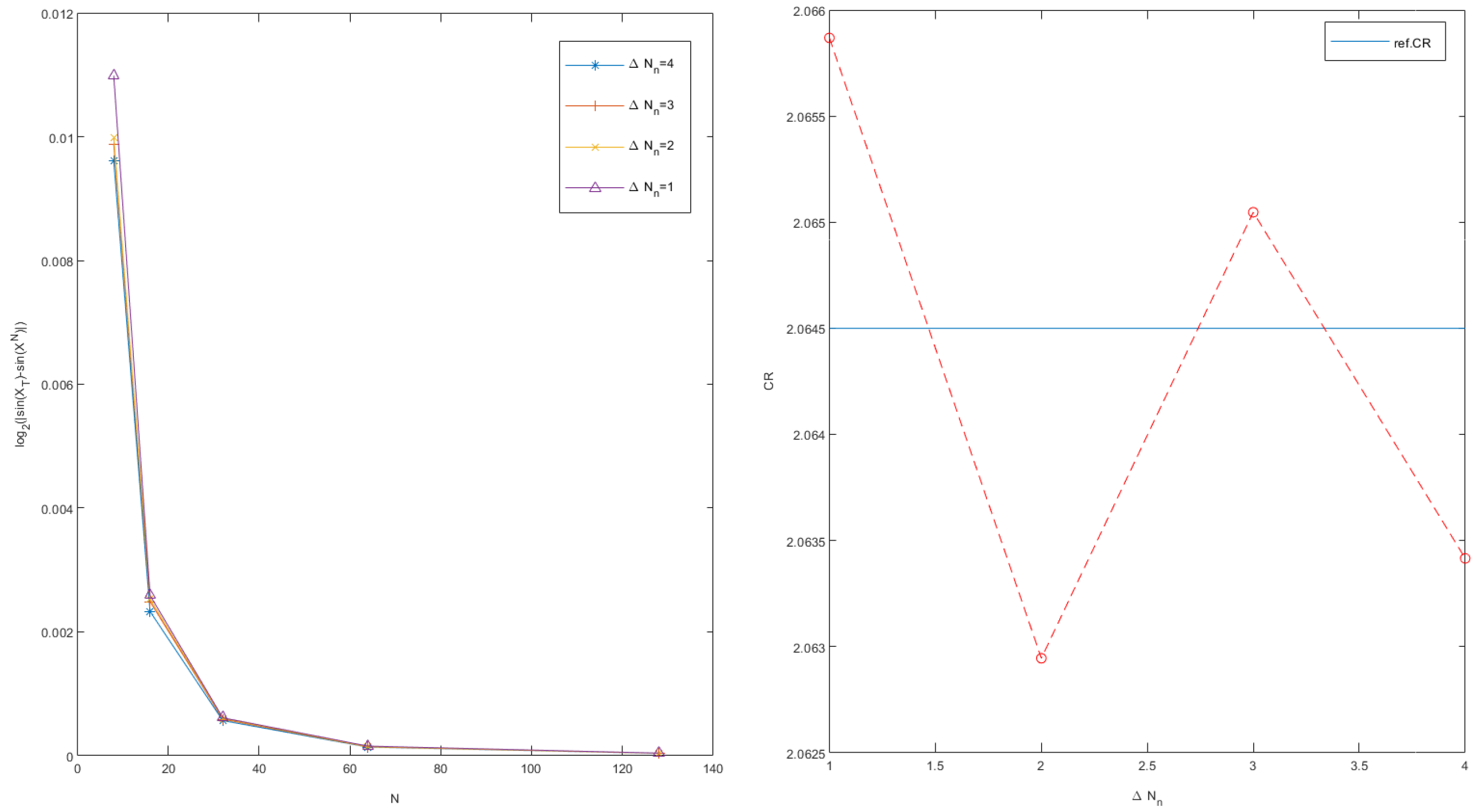
Example 3.

Consider the O-U process with pure jump:

$$\left\{\begin{array}{c}{X}_t=X_0-{\int }_0^{t}a{X}_{s}ds+h{\int }_0^t{\int }_{\mathcal{E}}e\tilde{N}(de,ds),\hfill \\ X_0=20,\hfill \end{array}\right.$$

(29)

where $\tilde{N}(de,ds)$ is one-dimensional compensated poisson process with $\gamma (e)=1$, $\mathcal{E}=[0,1]$ and ${\lambda }_{\mathcal{E}}={\int }_0^{1}de=1$. Let $a=1.5$, $h=0.01$, and $e\in U(0,1)$. Applying Itô formula to $e^{at}{X}_t,$ Equation (29) has the explicit solution

$$X_t=X_0{e}^{-at}+h{e}^{-at}{\int }_0^t{\int }_{\mathcal{E}}{e}^{as}e\tilde{N}(de,ds).$$

For the model (29), by using Itô Taylor expansion, the new Scheme 5 is

$$\begin{array}{cc}\hfill X^{n+1}& =X^n-{\int }_{t_n}^{t_{n+1}}a{X}^{n}ds+h{\int }_{t_n}^{t_{n+1}}{\int }_{\mathcal{E}}e\tilde{N}(de,ds)+a^2{X}^n{\int }_{t_n}^{t_{n+1}}{\int }_{t_n}^{t}dsdt-ah{\int }_{t_n}^{t_{n+1}}{\int }_{t_n}^t{\int }_{\mathcal{E}}e\tilde{N}(de,ds)dt,\hfill \end{array}$$

Using the fact that ${\int }_{t_n}^{t_{n+1}}{\int }_{\mathcal{E}}e\tilde{N}(de,ds)=\sum _{k=1}^{∆N_n}{\xi }_k,$ ${\int }_{\mathcal{E}}e\lambda (de)={\int }_0^{1}ede=\frac{1}{2}$ and

$$\begin{array}{cc}\hfill {\int }_{t_n}^{t_{n+1}}{\int }_{t_n}^t{\int }_{\mathcal{E}}e\tilde{N}(de,ds)dt& ={\int }_{t_n}^{t_{n+1}}{\int }_{t_n}^t{\int }_{\mathcal{E}}eN(de,ds)dt-{\int }_{t_n}^{t_{n+1}}{\int }_{t_n}^t{\int }_{\mathcal{E}}e\lambda (de)dsdt\hfill \\ \hfill & =\sum _{k=1}^{∆N_n}{\xi }_k(t_{n+1}-{\tau }_k)∆t-\frac{1}{4}{\lambda }_{\mathcal{E}}{(∆t)}^2,\hfill \end{array}$$

Scheme 5 becomes

$$\begin{array}{cc}\hfill X^{n+1}& =X^n-a{X}^n∆t+h\sum _{k=1}^{∆N_n}{\xi }_k-\frac{1}{2}h{\lambda }_{\mathcal{E}}∆t+\frac{1}{2}{a}^2{X}^n{(∆t)}^2-ah\left[\sum _{k=1}^{∆N_n}{\xi }_k(t_{n+1}-{\tau }_k)∆t-\frac{1}{4}{\lambda }_{\mathcal{E}}{(∆t)}^2\right],\hfill \end{array}$$

where ${\tau }_k$ is the kth jump time, ${\xi }_k$ is the kth jump mark, and the pairs $({\tau }_k,{\xi }_k)$ are uniformly distributed in the square $[0,1]\times [0,1]$.

In this example, the right of Figure 1 shows that, even if the jumps number $∆N_n$ increase in $[t_n,t_{n+1}]$, the convergence rate of Scheme 5 can still achieve second order. Meanwhile, the left of Figure 1 presents that the global errors may have some difference with different $∆N_n$; a higher number of jumps accompanies less global error in numerical computing in $[t_n,t_{n+1}]$. Then, we conclude that there is a little impact of the random generation of the compound Poisson process.

Figure 1. (Left) The global errors for Example 3; and (Right) the convergence rates of $∆N_n=1$, $∆N_n=2$, $∆N_n=3$, and $∆N_n=4$.

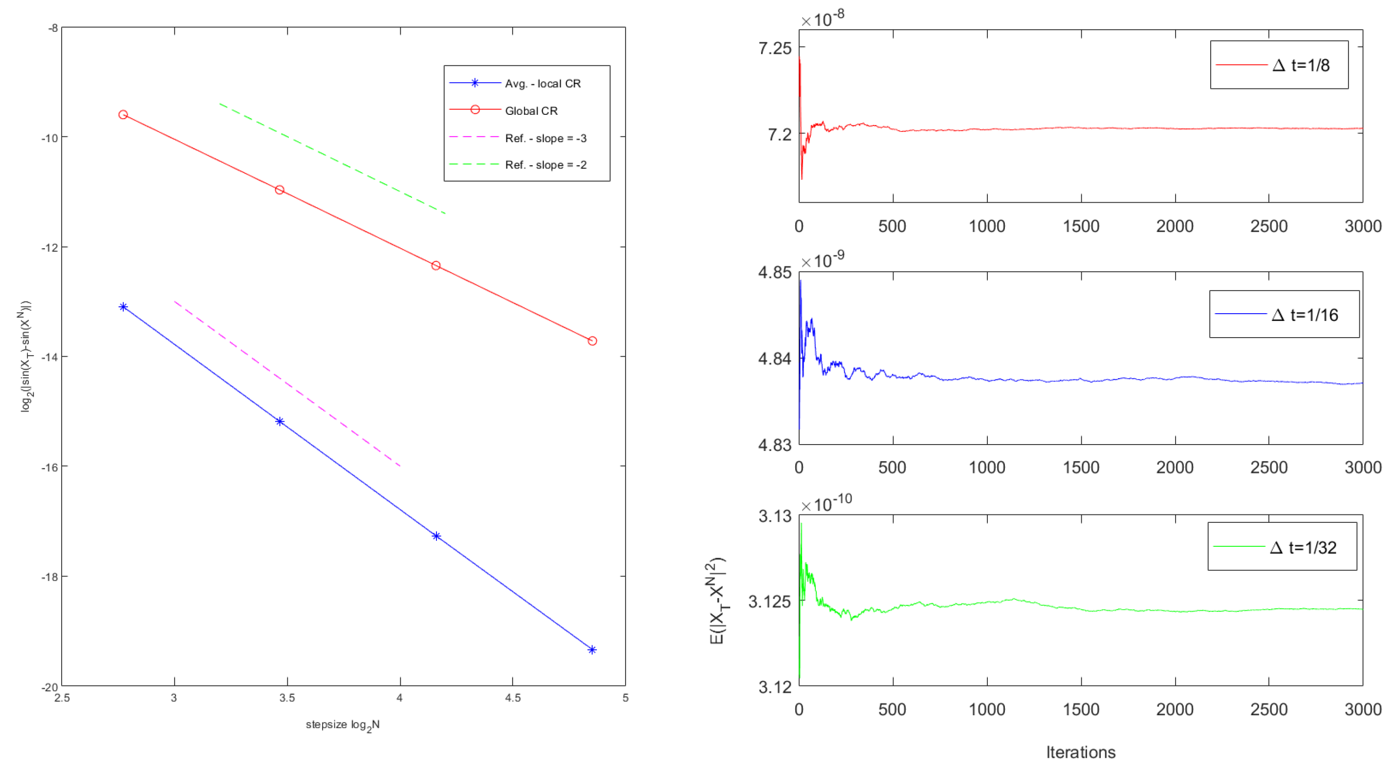
Example 4.

Consider the geometrical model with pure jump:

$$\left\{\begin{array}{c}{X}_t=X_0+{\int }_0^{t}a{X}_{s}ds+{\int }_0^t{\int }_{\mathcal{E}}h{X}_s\tilde{N}(de,ds),\hfill \\ X_0=0.1,\hfill \end{array}\right.$$

(30)

where $\tilde{N}(de,ds)$ is a one-dimensional compensated Poisson process with ${\lambda }_{\mathcal{E}}=1$. Let $a=0.8$ and $h=0.01$; the equation has the explicit solution by using Itô formula

$$X_t=X_{0}exp\left\{{\int }_0^t(a-{\lambda }_{\mathcal{E}}h)ds+{\int }_0^t{\int }_{\mathcal{E}}ln(1+h)N(de,ds)\right\}.$$

For the model (30), the new Scheme 5 is

$$\begin{array}{cc}\hfill X^{n+1}=& X^n+a{X}^n∆t+h{X}^n∆{\tilde{N}}_n+\frac{1}{2}{a}^2{X}^n{(∆t)}^2+ah{X}^n∆{\tilde{N}}_n∆t+\frac{1}{2}{h}^2{X}^n({(∆{\tilde{N}}_n)}^2-{\lambda }_{\mathcal{E}}∆t-∆{\tilde{N}}_n).\hfill \end{array}$$

In this pure jump geometrical model, we apply Scheme 5 to compute $\mathbb{E}[X^N]$ using 5000 sample trajectories. In Table 1, we obtain the scheme errors with $∆t=\{2^{-3},2^{-4},2^{-5},2^{-6},2^{-7}\}$. In addition, we show the global errors and average local errors of the scheme have the convergence rates of global second-order and average local third-order, respectively. Meanwhile, we intuitively display the accuracy of Scheme 5 from the left of Figure 2, where the two coordinate axes are ${log}_2∆t$ and ${log}_2|\phi (X_{t_N})-\phi (X^N)|$. On the other hand, from the right of Figure 2, we verify the result of mean-square convergence stability with $\mathbb{E}[{|\phi (X_{t_N})-\phi (X^N)|}^2]$.

Table 1. Errors and convergence rates of Scheme 5 with the parameters of Example 4.

N	Global Errors	CR	Avg. Local Errors	CR
8	2.618$\times {10}^{-4}$		1.664$\times {10}^{-5}$
16	6.785$\times {10}^{-5}$	1.9482	2.052$\times {10}^{-6}$	3.0197
32	1.724$\times {10}^{-5}$	1.9622	2.544$\times {10}^{-7}$	3.0156
64	4.345$\times {10}^{-6}$	1.9716	3.166$\times {10}^{-8}$	3.0125
128	1.101$\times {10}^{-6}$	1.9751	3.987$\times {10}^{-9}$	3.0072

Figure 2. (Left) The global convergence rates and average local convergence rate for Example 4 with both referenced slope of 2 and 3; and (Right) the mean-square convergence stability of the schemes with $∆t=1/8$, $∆t=1/16$, and $∆t=1/32$.

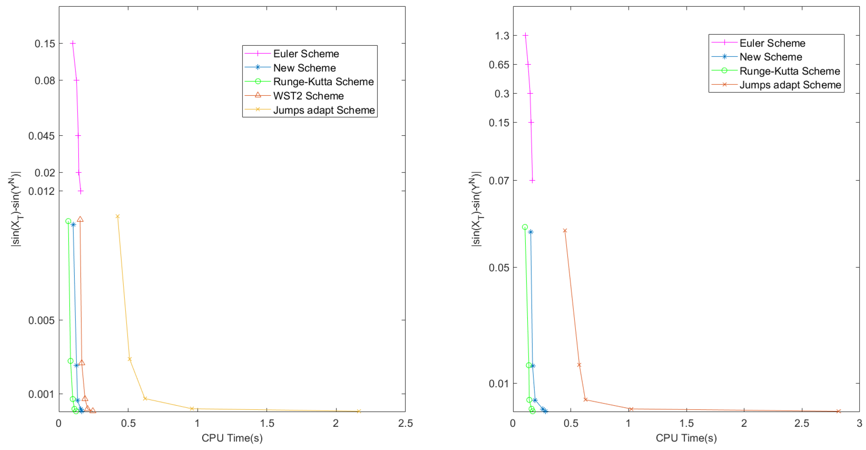
To illustrate the advantages of Scheme 5 in computational efficiency, we also apply Euler Scheme, Runge–Kutta Scheme, WST2 Scheme, and Jump-adapted Scheme to solve Equation (30). The global errors and convergence rates of the schemes are displayed in Table 2 and the left of Figure 3 displays the sample global errors and the corresponding CPU time of the Euler Scheme, Scheme 5, Runge–Kutta Scheme, WST2 Scheme, and Jump-adapted Scheme with $X_0=0.5$, $a=1.5$, $h=0.001$.

Table 2. Errors and convergence rates of schemes with the parameters of Example 4.

N	8	16	32	64	128	CR	Time(s)
Euler Scheme	1.494$\times {10}^{-1}$	8.023$\times {10}^{-2}$	4.564$\times {10}^{-2}$	2.242$\times {10}^{-2}$	1.180$\times {10}^{-2}$	0.916	0.64640
New Scheme 5	1.015$\times {10}^{-2}$	2.531$\times {10}^{-3}$	6.352$\times {10}^{-4}$	1.592$\times {10}^{-4}$	3.701$\times {10}^{-5}$	2.019	0.69348
Runge–Kutta Scheme	1.035$\times {10}^{-2}$	2.772$\times {10}^{-3}$	7.037$\times {10}^{-4}$	1.709$\times {10}^{-4}$	4.082$\times {10}^{-5}$	1.999	0.59267
WST2 Scheme	1.042$\times {10}^{-2}$	2.656$\times {10}^{-3}$	7.015$\times {10}^{-4}$	1.688$\times {10}^{-4}$	4.162$\times {10}^{-5}$	1.991	0.71448
Jump-adapted Scheme	1.062$\times {10}^{-2}$	2.875$\times {10}^{-3}$	7.315$\times {10}^{-4}$	1.807$\times {10}^{-4}$	4.456$\times {10}^{-5}$	1.9718	4.67431

Figure 3. (Left) The global samples errors and CPU time of Example 4; and (Right) the global samples errors and CPU time of Example 5.

Example 5.

Consider the nonlinear model with pure jump:

$$\left\{\begin{array}{c}{X}_t=X_0+{\int }_0^t(a{X}_s+as)ds+{\int }_0^t{\int }_{\mathcal{E}}h\sqrt{X_s}\tilde{N}(de,ds),\hfill \\ X_0=2,\hfill \end{array}\right.$$

(31)

where $\tilde{N}(de,ds)$ is a one-dimensional compensated Poisson process with ${\lambda }_{\mathcal{E}}=1$. Let $a=1.5$ and $h=0.002$. The new Scheme 5 is

$$\begin{array}{cc}\hfill X^{n+1}& =X^n+(a{X}^n+a{t}_n)∆t+h\sqrt{X^n}∆{\tilde{N}}_n+\frac{1}{2}\left(a+a^2{X}^n+a^2{t}_n\right){(∆t)}^2+\frac{1}{2}ah\sqrt{X^n}∆{\tilde{N}}_n∆t\hfill \\ \hfill & +\frac{1}{2}\left(\frac{ah{X}^n+ah{t}_n}{2\sqrt{X^n}}+\left(h\sqrt{X^n+\sqrt{X^n}}-h\sqrt{X^n}-\frac{1}{2}{h}^2\right){\lambda }_{\mathcal{E}}\right)∆t∆{\tilde{N}}_n\hfill \\ \hfill & +\frac{1}{2}\left(h\sqrt{X^n+\sqrt{X^n}}-h\sqrt{X^n}\right)\left({(∆{\tilde{N}}_n)}^2-{\lambda }_{\mathcal{E}}∆t-∆{\tilde{N}}_n\right).\hfill \end{array}$$

In this experiment, we give a nonlinear example which the drift coefficients satisfy Lipschitz condition. Since the exact solution of Equation (31) cannot be expressed explicitly, we set a small time step of $∆t=2^{-18}$ as the exact reference solution.

We give the errors and the convergence rates with different parameters of Example 5 in Table 3 and Figure 3 (right), for the WST2 Scheme. When $∆t<2^{-7}$, the accuracy of reference solution is worse (refer Liu and Li [21]). Therefore, we give the comparison of errors and convergence rates, which includes Euler Scheme, Scheme 5, Runge–Kutta Scheme, and Jump-adapted Scheme.

Table 3. Errors and convergence rates of schemes with the parameters of Example 5.

N	8	16	32	64	128	CR	Time(s)
Euler Scheme	1.278	6.647$\times {10}^{-1}$	3.153$\times {10}^{-1}$	1.493$\times {10}^{-1}$	7.194$\times {10}^{-2}$	1.0456	0.70768
New Scheme 5	6.210$\times {10}^{-2}$	1.596$\times {10}^{-2}$	4.172$\times {10}^{-3}$	1.005$\times {10}^{-3}$	2.597$\times {10}^{-4}$	1.9793	0.98609
Runge–Kutta Scheme	6.383$\times {10}^{-2}$	1.614$\times {10}^{-2}$	4.202$\times {10}^{-3}$	1.094$\times {10}^{-3}$	2.693$\times {10}^{-4}$	1.9960	0.71030
Jump-adapted Scheme	6.273$\times {10}^{-2}$	1.627$\times {10}^{-2}$	4.249$\times {10}^{-3}$	1.083$\times {10}^{-3}$	2.605$\times {10}^{-4}$	1.9732	5.48587

5. Conclusions

In this paper, we propose a new simplified weak second-order numerical scheme for solving stochastic differential equations with jumps. By using trapezoidal rule and the integration-by-parts formula of Malliavin calculus, we theoretically prove that the numerical scheme has second-order convergence rate. In numerical experiments, we used three examples to verify the convergence of our scheme. Meanwhile, we compared the computational time, programming complexity and precision of our scheme with other schemes, such as Euler Scheme, Runge–Kutta Scheme, WST2 Scheme and Jump-adapted Scheme and found our new scheme can be easily computed and consume less run time.