
An Analysis of a KNN Perturbation Operator: An Application to the Binarization of Continuous Metaheuristics


Abstract
1. Introduction
- Inspired by the work in [13], an improvement is proposed to the binarization technique that uses transfer functions, developed in [14], with the objective of metaheuristics which were defined to function in continuous spaces, efficiently solve COPs. This article includes the K-nearest neighbor technique to improve the diversification and intensification properties of a specific metaheuristic. Unlike in [13], in which the perturbation operator is integrated with the k-means clustering technique, in this article the perturbation operator is integrated with transfer functions, and these functions perform the binarization of the continuous metaheuristics. For this work, the Cuckoo Search (CS) metaheuristic was used. This algorithm was chosen due to its ease in parameter tuning, in addition to the existence of basic theoretical models of convergence.
- Unlike in [13], in which the multidimensional knapsack problem was tackled, this article addresses the set covering problem (SCP). This combinatorial problem has been widely studied and, because of that, instances of different difficulties are available which facilitate our analysis. In this work, we have chosen to use large size instances in order to adequately evaluate the contribution of the KNNperturbation operator.
- For a suitable evaluation of our KNN perturbation operator, we first use a parameter estimation methodology proposed in [15] with the goal to find the best metaheuristic configurations. Later, experiments are carried out to get insight into the contribution of the KNN operator. Finally, our hybrid algorithm is compared to the state-of-the-art general binarization methods. The numerical results show that our proposal achieves highly competitive results.
2. Related Work
2.1. Hybridizing Metaheuristics with Machine Learning
- The first front is to apply ML at the level of the problem to be solved. This first front considers obtaining expert knowledge about the characteristics of the data of the problem under consideration. The problem model can be reformulated or it can be broken down to achieve a more efficient and effective solution. The good knowledge of the characteristics allows to design efficient metaheuristics and to understand the behavior of the algorithms. The benefits are varied, ranging from allowing the selection of an appropriate metaheuristic for each type of problem [25] to the possibility of finding an appropriate configuration of parameters [26]. For the knowledge of the ML characteristics it has several methods that can be used: neural networks [27], Bayesian networks [28], regression trees [26], support vector regression [29], Gaussian process [30], ridge regression [25], and random forest [30].
- The second front is to apply ML at the level of the components of metaheuristics. On this front, ML can be used to find suitable search components (or to find a good configuration of parameter values the latter in sin is an optimization problem. ML can be used to find good initial solutions which allows to improve the quality of the solutions and reduce processing costs since currently the initial solutions are randomly generated and of not very good quality [31]. Another participation of ML is in the design of the search operators: constructive, unary, binary, indirect, intensification, and diversification. Furthermore, ML can be present in the important task of finding a good configuration of parameters as this activity has direct impact on the performance of the algorithm [32]. Usually, the assignment of parameters is done by applying the technique of trial and error, which undoubtedly causes a loss of resources, especially time [33]. The number of parameters can vary between one metaheuristic and another, which makes experience an important factor.In general there are two major groups of parameters: those where the values are given before the execution of the algorithm known as static or offline parameters and there are also the parameters where the values are assigned during the execution of the algorithm also known as online or dynamic parameter setting. In the case of the offline parameters, the following ML methodologies can be used: unsupervised learning, supervised learning, and surrogate-based optimization. For the case of sustainable wall design, the k-means unsupervised learning technique was used in [34] to allow algorithms that work naturally in continuous spaces to solve a combinatorial wall design problem. In the allocation of resources, the db-scan technique was used in [35], to solve the multidimensional knapsack problem. For the case of online parameter value assignment, where parameters are changed during the execution of the algorithm, the knowledge obtained during the search can serve as information to dynamically change the values of the parameters during its execution using ML methodologies, as they are Sequential learning approach, Classification/regression approach and Clustering approach. In [36], an algorithm has been proposed in order to carry out an intelligent initiation of algorithms based on populations. In this article, clustering techniques are used for the initiation. The results indicated that the proposed intelligent sampling has a significant impact, as it improves the performance of the algorithms with which it has been integrated. The integration of the k-nearest neighbors technique with a quantum cuckoo search algorithm was proposed in [37]. In this case, the proposed hybrid algorithm was applied to the multidimensional knapsack problem. The results showed that the hybrid algorithm is more robust than the original version.
- A third front is the choice of the best algorithm within a portfolio arranged for a certain problem. There are several metaheuristics to solve complex problems which may have common characteristics among them. For this reason, we can think of selecting an adequate metaheuristic to solve a problem with certain characteristics. We know that there is not a single metaheuristic that can solve a wide variety of problems, so the use of an alternative is to select from a portfolio of algorithms [38]. ML is a good tool for an adequate selection of the algorithm [39]. In this case, we can distinguish between offline learning where information is gathered from a series of instances in a previous form with the purpose of replicating new instances considering three approaches: classification, regression, and clustering. On the other hand, there is the online approach, which has the potential to be adaptive. Additionally, there are some hybrid approaches [40]. In [41], a cooperative strategy was implemented with the aim of land mine detection. The results of the strategy show good detection precision and robustness to environmental changes and data sets.
2.2. Related Binarization Work
- Transfer Function-Binarization. This two-step binarization technique is widely used due to its low implementation cost. In the first step, transfer functions (TF) are used which produce values between 0 and 1 and then in the second step convert these values into binary using rules that allow to leave as value 0 or 1.There are two groups of transfer functions which are associated with the form of the function, which can be either S or V. A TF takes values of and generates transition probability values of . These were used to allow PSO to work with binary problems by relating the speed of particles to a transition probability. In PSO a particle is a solution which in each iteration has a position and velocity which is given by the difference of position between iterations. On the other hand, there are several rules to convert these values to binary among these are Complement, Static probability, Elitist, Elitist Roulette, or Monte Carlo.
- Angle Modulation-Rule. This binary technique has as a first step the use of Angle Modulation was used for phase and frequency modulation of the signal in the telecommunications industry [46]. It belongs to the family of four-parameter trigonometric functions by which it controls the frequency and displacement of the trigonometric function.In PSO, binary heuristic optimization applied to a set of reference functions was used for the first time [47].Consider an n-dimensional binary problem, and let be a solution. First of all, we define a four-dimensional search space. In this space, each dimension corresponds to a coefficient of Equation (1). As a first stage, using the four-dimensional space, we get a function. Specifically, from every tuple in this space, we get a . This corresponds to a trigonometric function.In the second stage, binarization, for each element , the rule (2) is applied and getting an n-dimensional binary solution.Then, for each initial 4-dimensional solution , we obtain a binary n-dimensional solution that is a feasible solution of our n-binary problem. In [48], the authors successfully applied to network reconfiguration problems multi-user detection in multi-carrier wireless broadband system [49], the antenna position problem [50], and N-queens problems [51].
- Quantum binary. In reviewing the areas of quantum and evolutionary computing we can distinguish three types of algorithms [52]:
- Quantum evolutionary algorithms: In these methods, EC algorithms are used in order to apply them in quantum computing.
- Evolutionary-based quantum algorithms: The objective of these methods is to automate the generation of new quantum algorithms. This automation is done using evolutionary algorithms.
- Quantum-inspired evolutionary algorithms: This category adapts concepts obtained from quantum computing in order to strengthen the EC algorithms.
The quantum binary approach is an evolutionary algorithm that adapts the concepts of q-bits and overlap used in quantum computing applied to traditional computers.The position of a feasible solution is given by and a quantum bit vector q where in this approach the probability of change Q is the probability that takes the value 1. For each dimension, a random number between [0.1] is generated and compared to : if , then ; otherwise, . The updating mechanism of the Q vector is specific to each metaheuristic.
3. The Set Covering Problem
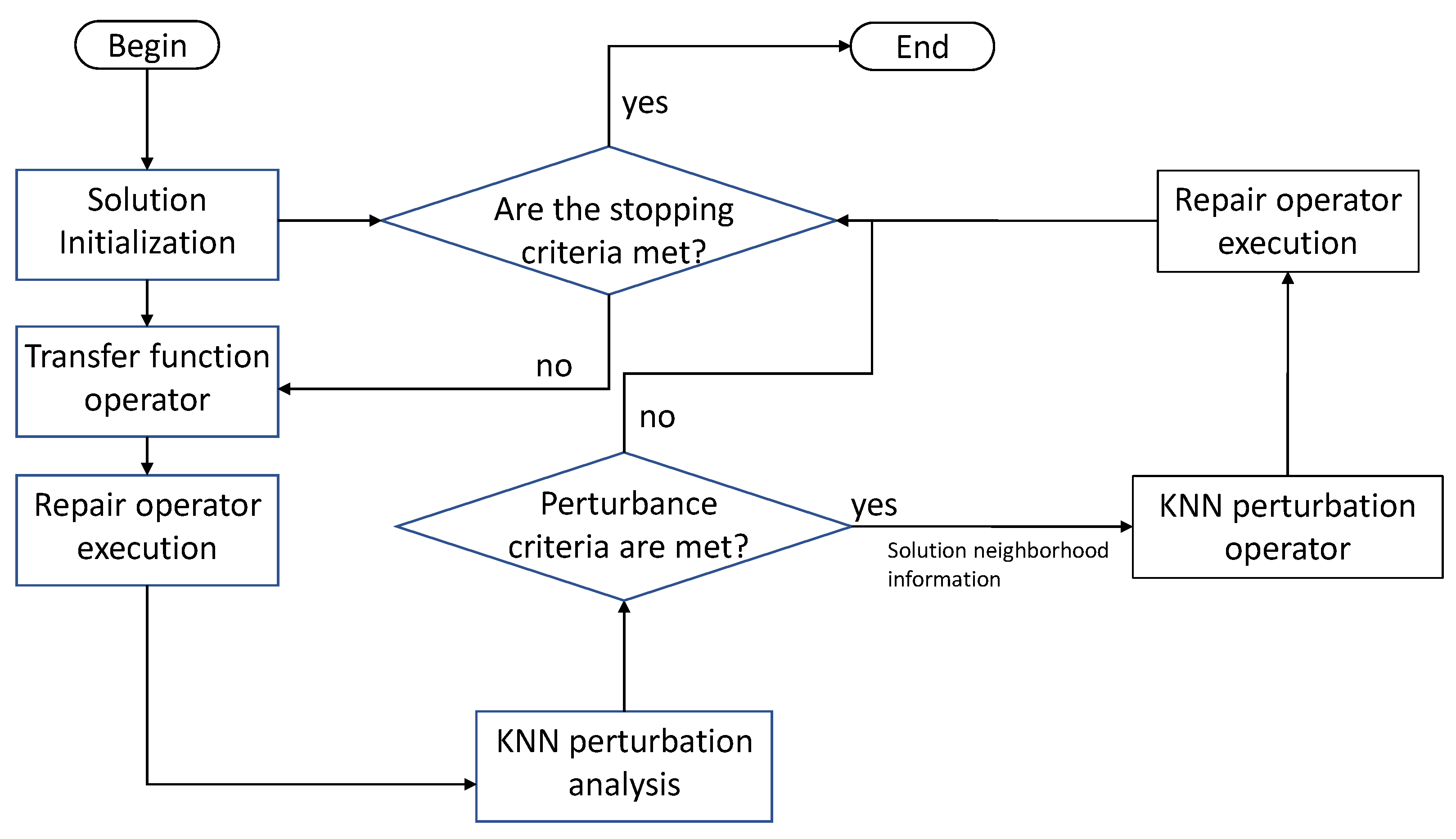
4. The Binary KNN Perturbed Algorithm
4.1. Initialization Operator
| Algorithm 1 Init Operator |
|
4.2. KNN Perturbation Analysis Module
| Algorithm 2 KNN perturbation analysis module |
|
4.3. KNN Perturbation Operator
| Algorithm 3 KNN Perturbation operator |
|
4.4. Transfer Function Operator
4.5. Repair Operator
| Algorithm 4 Repair Operator |
|
4.6. Heuristic Function
| Algorithm 5 Heuristic function |
|
5. Numerical Results
5.1. Parameter Settings
- The percentage deviation of the best value resulting in ten runs compared with the best-known value:
- The percentage deviation of the worst value resulting in ten runs compared to the best-known value:
- The average percentage deviation value resulting in ten runs compared with the best-known value:
- The convergence time in each experiment is standardized using Equation (16).
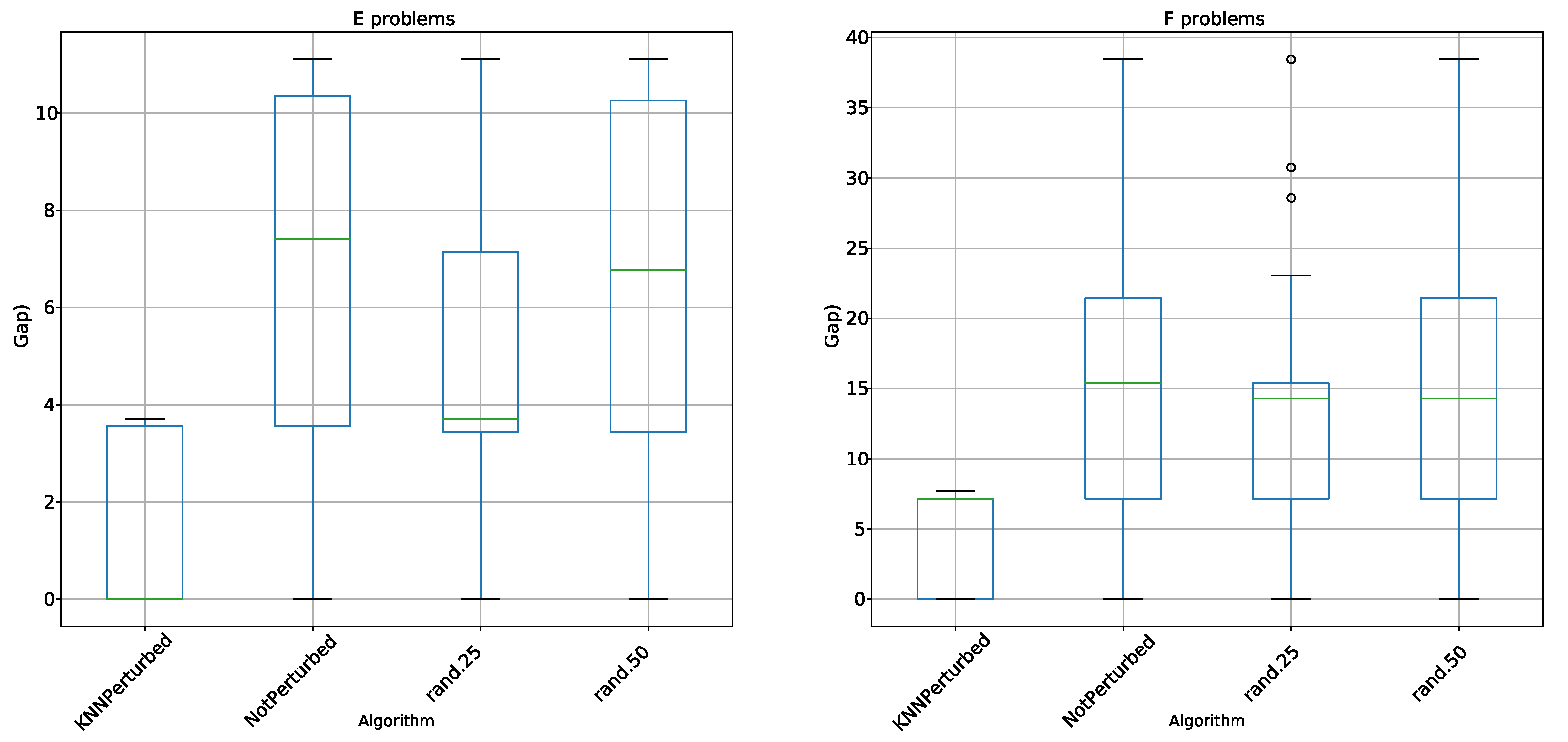
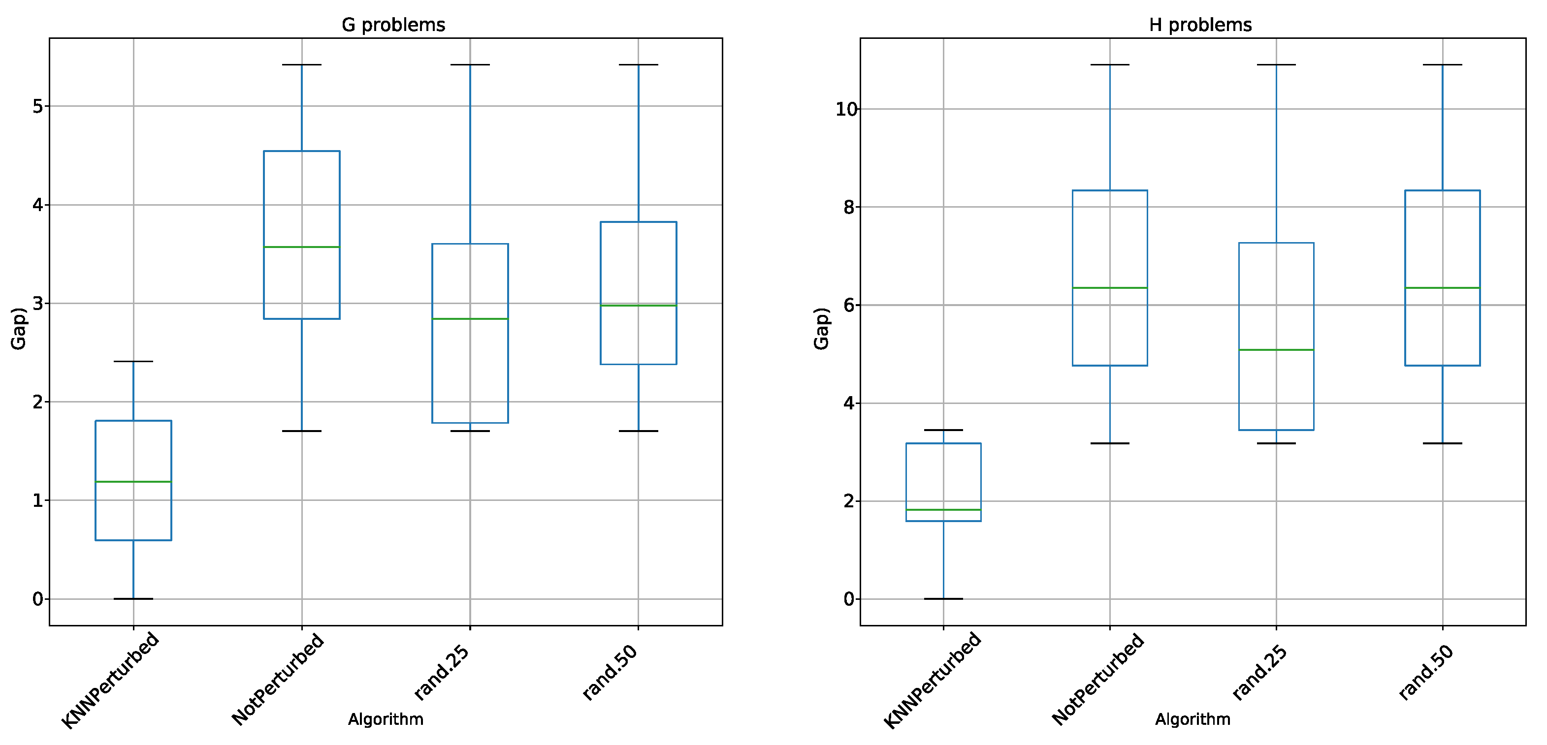
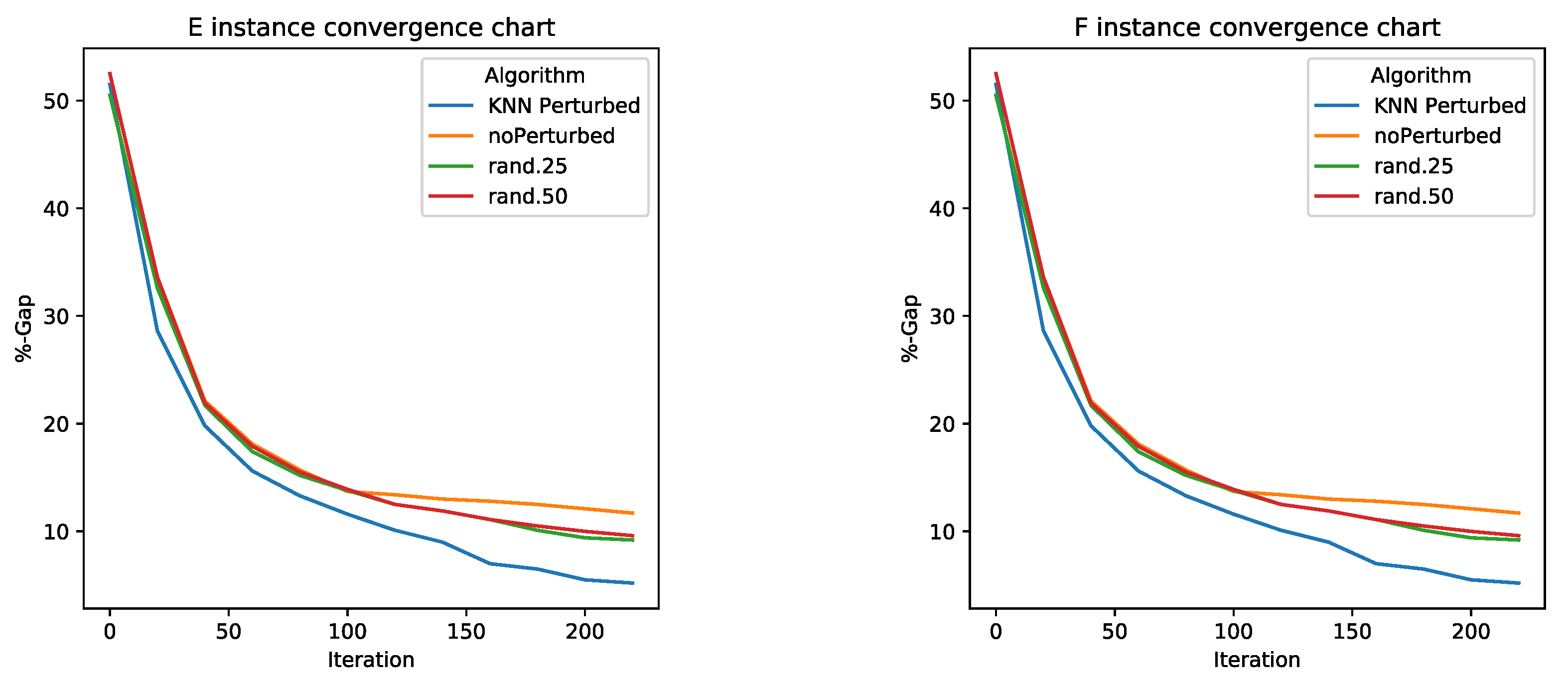
5.2. Perturbation Operator Analysis
5.3. Comparisons
- KNN perturbation in the 4 types of problems outperforms BBH and BCS. These techniques use transfer functions as a method of binarization, the same methods used by KNN perturbation.
- KNN perturbation outperforms db-scan-CS only on instance G. In all other instances, db-scan-CS performs better. db-scan-CS uses a binarization mechanism based on db-scan which adapts iteration to iteration. However, the difference is not statistically significant.
6. Conclusions
Author Contributions
Funding
Data Availability Statement
Conflicts of Interest
References
- Al-Madi, N.; Faris, H.; Mirjalili, S. Binary multi-verse optimization algorithm for global optimization and discrete problems. Int. J. Mach. Learn. Cybern. 2019, 10, 3445–3465. [Google Scholar] [CrossRef]
- García, J.; Moraga, P.; Valenzuela, M.; Crawford, B.; Soto, R.; Pinto, H.; Peña, A.; Altimiras, F.; Astorga, G. A Db-Scan Binarization Algorithm Applied to Matrix Covering Problems. Comput. Intell. Neurosci. 2019, 2019, 3238574. [Google Scholar] [CrossRef] [PubMed]
- Guo, H.; Liu, B.; Cai, D.; Lu, T. Predicting protein–protein interaction sites using modified support vector machine. Int. J. Mach. Learn. Cybern. 2018, 9, 393–398. [Google Scholar] [CrossRef]
- Korkmaz, S.; Babalik, A.; Kiran, M.S. An artificial algae algorithm for solving binary optimization problems. Int. J. Mach. Learn. Cybern. 2018, 9, 1233–1247. [Google Scholar] [CrossRef]
- García, J.; Martí, J.V.; Yepes, V. The Buttressed Walls Problem: An Application of a Hybrid Clustering Particle Swarm Optimization Algorithm. Mathematics 2020, 8, 862. [Google Scholar] [CrossRef]
- Yepes, V.; Martí, J.V.; García, J. Black Hole Algorithm for Sustainable Design of Counterfort Retaining Walls. Sustainability 2020, 12, 2767. [Google Scholar] [CrossRef]
- Caserta, M.; Voß, S. Metaheuristics: Intelligent Problem Solving. In Matheuristics: Hybridizing Metaheuristics and Mathematical Programming; Maniezzo, V., Stützle, T., Voß, S., Eds.; Springer: Boston, MA, USA, 2010; pp. 1–38. [Google Scholar]
- Talbi, E.G. Combining metaheuristics with mathematical programming, constraint programming and machine learning. Ann. Oper. Res. 2016, 240, 171–215. [Google Scholar] [CrossRef]
- Juan, A.A.; Faulin, J.; Grasman, S.E.; Rabe, M.; Figueira, G. A review of simheuristics: Extending metaheuristics to deal with stochastic combinatorial optimization problems. Oper. Res. Perspect. 2015, 2, 62–72. [Google Scholar] [CrossRef]
- Chou, J.S.; Nguyen, T.K. Forward Forecast of Stock Price Using Sliding-Window Metaheuristic-Optimized Machine-Learning Regression. IEEE Trans. Ind. Inform. 2018, 14, 3132–3142. [Google Scholar] [CrossRef]
- Zheng, B.; Zhang, J.; Yoon, S.W.; Lam, S.S.; Khasawneh, M.; Poranki, S. Predictive modeling of hospital readmissions using metaheuristics and data mining. Expert Syst. Appl. 2015, 42, 7110–7120. [Google Scholar] [CrossRef]
- de León, A.D.; Lalla-Ruiz, E.; Melián-Batista, B.; Moreno-Vega, J.M. A Machine Learning-based system for berth scheduling at bulk terminals. Expert Syst. Appl. 2017, 87, 170–182. [Google Scholar] [CrossRef]
- García, J.; Lalla-Ruiz, E.; Voß, S.; Droguett, E.L. Enhancing a machine learning binarization framework by perturbation operators: Analysis on the multidimensional knapsack problem. Int. J. Mach. Learn. Cybern. 2020, 11, 1951–1970. [Google Scholar] [CrossRef]
- García, J.; Crawford, B.; Soto, R.; Astorga, G. A clustering algorithm applied to the binarization of swarm intelligence continuous metaheuristics. Swarm Evol. Comput. 2019, 44, 646–664. [Google Scholar] [CrossRef]
- García, J.; Crawford, B.; Soto, R.; Castro, C.; Paredes, F. A k-means binarization framework applied to multidimensional knapsack problem. Appl. Intell. 2018, 48, 357–380. [Google Scholar] [CrossRef]
- Dokeroglu, T.; Sevinc, E.; Kucukyilmaz, T.; Cosar, A. A survey on new generation metaheuristic algorithms. Comput. Ind. Eng. 2019, 137, 106040. [Google Scholar] [CrossRef]
- Geem, Z.W.; Kim, J.; Loganathan, G. A New Heuristic Optimization Algorithm: Harmony Search. Simulation 2001, 76, 60–68. [Google Scholar] [CrossRef]
- Karaboga, D. An Idea Based on Honey Bee Swarm for Numerical Optimization; Technical Report, Technical Report-tr06; Erciyes university, Engineering Faculty, Computer Engineering Department: Kayseri, Turkey, 2005. [Google Scholar]
- Yang, X.S.; Deb, S. Cuckoo search via Lévy flights. In Proceedings of the 2009 World Congress on Nature & Biologically Inspired Computing (NaBIC), Coimbatore, India, 9–11 December 2009; pp. 210–214. [Google Scholar]
- Rashedi, E.; Nezamabadi-Pour, H.; Saryazdi, S. GSA: A gravitational search algorithm. Inf. Sci. 2009, 179, 2232–2248. [Google Scholar] [CrossRef]
- Rao, R.V.; Savsani, V.J.; Vakharia, D. Teaching–learning-based optimization: A novel method for constrained mechanical design optimization problems. Comput.-Aided Des. 2011, 43, 303–315. [Google Scholar] [CrossRef]
- Gandomi, A.H.; Alavi, A.H. Krill herd: A new bio-inspired optimization algorithm. Commun. Nonlinear Sci. Numer. Simul. 2012, 17, 4831–4845. [Google Scholar] [CrossRef]
- Cuevas, E.; Cienfuegos, M. A new algorithm inspired in the behavior of the social-spider for constrained optimization. Expert Syst. Appl. 2014, 41, 412–425. [Google Scholar] [CrossRef]
- Abdel-Basset, M.; Abdel-Fatah, L.; Sangaiah, A.K. Metaheuristic algorithms: A comprehensive review. In Computational Intelligence for Multimedia Big Data on the Cloud with Engineering Applications; Elsevier: Amsterdam, The Netherlands, 2018; pp. 185–231. [Google Scholar]
- Xu, L.; Hutter, F.; Hoos, H.H.; Leyton-Brown, K. SATzilla: Portfolio-based algorithm selection for SAT. J. Artif. Intell. Res. 2008, 32, 565–606. [Google Scholar] [CrossRef]
- Bartz-Beielstein, T.; Markon, S. Tuning search algorithms for real-world applications: A regression tree based approach. In Proceedings of the 2004 Congress on Evolutionary Computation (IEEE Cat. No.04TH8753), Portland, OR, USA, 19–23 June 2004; Volume 1, pp. 1111–1118. [Google Scholar]
- Smith-Miles, K.; van Hemert, J. Discovering the suitability of optimisation algorithms by learning from evolved instances. Ann. Math. Artif. Intell. 2011, 61, 87–104. [Google Scholar] [CrossRef]
- Peña, J.M.; Lozano, J.A.; Larrañaga, P. Globally multimodal problem optimization via an estimation of distribution algorithm based on unsupervised learning of Bayesian networks. Evol. Comput. 2005, 13, 43–66. [Google Scholar] [CrossRef] [PubMed]
- Bischl, B.; Mersmann, O.; Trautmann, H.; Preuß, M. Algorithm selection based on exploratory landscape analysis and cost-sensitive learning. In Proceedings of the 14th Annual Conference on Genetic And Evolutionary Computation, Philadelphia, PA, USA, 7–11 July 2012; pp. 313–320. [Google Scholar]
- Hutter, F.; Xu, L.; Hoos, H.H.; Leyton-Brown, K. Algorithm runtime prediction: Methods & evaluation. Artif. Intell. 2014, 206, 79–111. [Google Scholar]
- Kazimipour, B.; Li, X.; Qin, A.K. A review of population initialization techniques for evolutionary algorithms. In Proceedings of the 2014 IEEE Congress on Evolutionary Computation (CEC), Beijing, China, 6–11 July 2014; pp. 2585–2592. [Google Scholar]
- De Jong, K. Parameter setting in EAs: A 30 year perspective. In Parameter Setting in Evolutionary Algorithms; Springer: Adelaide, Australia, 2007; pp. 1–18. [Google Scholar]
- Eiben, A.E.; Smit, S.K. Parameter tuning for configuring and analyzing evolutionary algorithms. Swarm Evol. Comput. 2011, 1, 19–31. [Google Scholar] [CrossRef]
- García, J.; Yepes, V.; Martí, J.V. A Hybrid k-Means Cuckoo Search Algorithm Applied to the Counterfort Retaining Walls Problem. Mathematics 2020, 8, 555. [Google Scholar] [CrossRef]
- García, J.; Moraga, P.; Valenzuela, M.; Pinto, H. A db-Scan Hybrid Algorithm: An Application to the Multidimensional Knapsack Problem. Mathematics 2020, 8, 507. [Google Scholar] [CrossRef]
- Poikolainen, I.; Neri, F.; Caraffini, F. Cluster-based population initialization for differential evolution frameworks. Inf. Sci. 2015, 297, 216–235. [Google Scholar] [CrossRef]
- García, J.; Maureira, C. A KNN quantum cuckoo search algorithm applied to the multidimensional knapsack problem. Appl. Soft Comput. 2021, 102, 107077. [Google Scholar] [CrossRef]
- Rice, J.R. The algorithm selection problem. In Advances in Computers; Elsevier: West Lafayette, IN, USA, 1976; Volume 15, pp. 65–118. [Google Scholar]
- Brazdil, P.; Carrier, C.G.; Soares, C.; Vilalta, R. Metalearning: Applications to data mining; Springer Science & Business Media: Houston, TX, USA, 2008. [Google Scholar]
- Burke, E.K.; Gendreau, M.; Hyde, M.; Kendall, G.; Ochoa, G.; Özcan, E.; Qu, R. Hyper-heuristics: A survey of the state of the art. J. Oper. Res. Soc. 2013, 64, 1695–1724. [Google Scholar] [CrossRef]
- Florez-Lozano, J.; Caraffini, F.; Parra, C.; Gongora, M. Cooperative and distributed decision-making in a multi-agent perception system for improvised land mines detection. Inf. Fusion 2020, 64, 32–49. [Google Scholar] [CrossRef]
- Crawford, B.; Soto, R.; Astorga, G.; García, J.; Castro, C.; Paredes, F. Putting Continuous Metaheuristics to Work in Binary Search Spaces. Complexity 2017, 2017, 8404231. [Google Scholar] [CrossRef]
- Taghian, S.; Nadimi-Shahraki, M.H.; Zamani, H. Comparative analysis of transfer function-based binary Metaheuristic algorithms for feature selection. In Proceedings of the 2018 International Conference on Artificial Intelligence and Data Processing (IDAP), Malatya, Turkey, 28–30 September 2018; pp. 1–6. [Google Scholar]
- Mafarja, M.; Aljarah, I.; Heidari, A.A.; Faris, H.; Fournier-Viger, P.; Li, X.; Mirjalili, S. Binary dragonfly optimization for feature selection using time-varying transfer functions. Knowl.-Based Syst. 2018, 161, 185–204. [Google Scholar] [CrossRef]
- Feng, Y.; An, H.; Gao, X. The importance of transfer function in solving set-union knapsack problem based on discrete moth search algorithm. Mathematics 2019, 7, 17. [Google Scholar] [CrossRef]
- Proakis, J.; Salehi, M. Communication Systems Engineering, 2nd ed.; Prentice Hall: Upper Saddle River, NJ, USA, 2002. [Google Scholar]
- Pampara, G.; Franken, N.; Engelbrecht, P. Combining particle swarm optimisation with angle modulation to solve binary problems. In Proceedings of the IEEE Congress on Evolutionary Computation Edinburgh, Scotland, UK, 2–5 September 2005; Volume 1, pp. 89–96. [Google Scholar]
- Liu, W.; Liu, L.; Cartes, D. Angle Modulated Particle Swarm Optimization Based Defensive Islanding of Large Scale Power Systems. In Proceedings of the IEEE Power Engineering Society Conference and Exposition in Africa, Johannesburg, South Africa, 16–20 July 2007; pp. 1–8. [Google Scholar]
- Swagatam, D.; Rohan, M.; Rupam, K. Multi-user detection in multi-carrier CDMA wireless broadband system using a binary adaptive differential evolution algorithm. In Proceedings of the 15th Annual Conference on Genetic and Evolutionary Computation, GECCO, Amsterdam, The Netherlands, July 2013; pp. 1245–1252. [Google Scholar]
- Dahi, Z.A.E.M.; Mezioud, C.; Draa, A. Binary bat algorithm: On the efficiency of mapping functions when handling binary problems using continuous-variable-based metaheuristics. In Proceedings of the IFIP International Conference on Computer Science and its Applications, Saida, Algeria, 20–21 May 2015; Springer: Cham, Switzerland, 2015; pp. 3–14. [Google Scholar]
- Leonard, B.J.; Engelbrecht, A.P. Frequency distribution of candidate solutions in angle modulated particle swarms. In Proceedings of the 2015 IEEE Symposium Series on Computational Intelligence, Cape Town, South Africa, 7–10 December 2015; pp. 251–258. [Google Scholar]
- Zhang, G. Quantum-inspired evolutionary algorithms: A survey and empirical study. J. Heurist. 2011, 17, 303–351. [Google Scholar] [CrossRef]
- Srikanth, K.; Panwar, L.K.; Panigrahi, B.; Herrera-Viedma, E.; Sangaiah, A.K.; Wang, G.G. Meta-heuristic framework: Quantum inspired binary grey wolf optimizer for unit commitment problem. Comput. Electr. Eng. 2018, 70, 243–260. [Google Scholar] [CrossRef]
- Hu, H.; Yang, K.; Liu, L.; Su, L.; Yang, Z. Short-term hydropower generation scheduling using an improved cloud adaptive quantum-inspired binary social spider optimization algorithm. Water Resour. Manag. 2019, 33, 2357–2379. [Google Scholar] [CrossRef]
- Gao, Y.J.; Zhang, F.M.; Zhao, Y.; Li, C. A novel quantum-inspired binary wolf pack algorithm for difficult knapsack problem. Int. J. Wirel. Mob. Comput. 2019, 16, 222–232. [Google Scholar] [CrossRef]
- Kumar, Y.; Verma, S.K.; Sharma, S. Quantum-inspired binary gravitational search algorithm to recognize the facial expressions. Int. J. Mod. Phys. C 2020, 31, 2050138. [Google Scholar] [CrossRef]
- Balas, E.; Padberg, M.W. Set partitioning: A survey. SIAM Rev. 1976, 18, 710–760. [Google Scholar] [CrossRef]
- Borneman, J.; Chrobak, M.; Della Vedova, G.; Figueroa, A.; Jiang, T. Probe selection algorithms with applications in the analysis of microbial communities. Bioinformatics 2001, 17, S39–S48. [Google Scholar] [CrossRef] [PubMed]
- Boros, E.; Hammer, P.L.; Ibaraki, T.; Kogan, A. Logical analysis of numerical data. Math. Program. 1997, 79, 163–190. [Google Scholar] [CrossRef]
- Garfinkel, R.S.; Nemhauser, G.L. Integer Programming; Wiley: New York, NY, USA, 1972; Volume 4. [Google Scholar]
- Balas, E.; Carrera, M.C. A dynamic subgradient-based branch-and-bound procedure for set covering. Oper. Res. 1996, 44, 875–890. [Google Scholar] [CrossRef]
- Beasley, J.E. An algorithm for set covering problem. Eur. J. Oper. Res. 1987, 31, 85–93. [Google Scholar] [CrossRef]
- John, B. A lagrangian heuristic for set-covering problems. Nav. Res. Logist. 1990, 37, 151–164. [Google Scholar]
- Beasley, J.E.; Chu, P.C. A genetic algorithm for the set covering problem. Eur. J. Oper. Res. 1996, 94, 392–404. [Google Scholar] [CrossRef]
- Iooss, B.; Lemaître, P. A review on global sensitivity analysis methods. In Uncertainty Management in Simulation-Optimization of Complex Systems; Springer: Boston, MA, USA, 2015; pp. 101–122. [Google Scholar]
- Soto, R.; Crawford, B.; Olivares, R.; Barraza, J.; Figueroa, I.; Johnson, F.; Paredes, F.; Olguín, E. Solving the non-unicost set covering problem by using cuckoo search and black hole optimization. Nat. Comput. 2017, 16, 213–229. [Google Scholar] [CrossRef]


| Parameters | Description | Value | Range |
|---|---|---|---|
| Perturbation operator coefficient | 25% | [20, 25, 30] | |
| N | Number of Nest | 20 | [20, 30,40] |
| K | Neighbours for the perturbation | 15 | [10, 15,20] |
| Step Length | 0.01 | 0.01 | |
| Levy distribution parameter | 1.5 | 1.5 | |
| Iterations | Maximum iterations | 1000 | [800, 900, 1000] |
| Instance | Best Known | .25 (Best) | .50 (Best) | Non Perturbed (Best) | KNN Perturbed (Best) | .25 (Avg) | .50 (avg) | Non Perturbed (Avg) | KNN (Avg) |
|---|---|---|---|---|---|---|---|---|---|
| E.1 | 29 | 30 | 30 | 31 | 29 | 30.6 | 30.9 | 31.8 | 29.4 |
| E.2 | 30 | 31 | 31 | 31 | 30 | 31.8 | 32.1 | 32.1 | 30.2 |
| E.3 | 27 | 28 | 29 | 29 | 27 | 28.7 | 29.5 | 29.7 | 27.6 |
| E.4 | 28 | 29 | 29 | 29 | 28 | 29.6 | 29.5 | 29.8 | 28.7 |
| E.5 | 28 | 28 | 28 | 28 | 28 | 28.7 | 28.8 | 29.1 | 28.4 |
| F.1 | 14 | 15 | 15 | 16 | 14 | 15.8 | 15.7 | 16.4 | 14.6 |
| F.2 | 15 | 15 | 15 | 15 | 15 | 15.7 | 16.1 | 15.9 | 15.2 |
| F.3 | 14 | 16 | 15 | 16 | 14 | 16.5 | 15.9 | 16.7 | 14.7 |
| F.4 | 14 | 15 | 16 | 16 | 14 | 15.4 | 16.5 | 16.7 | 14.8 |
| F.5 | 13 | 15 | 15 | 15 | 13 | 15.3 | 15.8 | 15.6 | 13.9 |
| G.1 | 176 | 179 | 180 | 182 | 176 | 180.1 | 181.2 | 183.2 | 177.2 |
| G.2 | 154 | 158 | 158 | 160 | 155 | 159.7 | 159.4 | 161.1 | 156.6 |
| G.3 | 166 | 171 | 172 | 171 | 168 | 172.4 | 173.2 | 172.3 | 169.2 |
| G.4 | 168 | 171 | 171 | 171 | 170 | 171.9 | 172.1 | 171.9 | 170.2 |
| G.5 | 168 | 171 | 171 | 172 | 168 | 172.1 | 172.0 | 173.2 | 168.6 |
| H.1 | 63 | 65 | 65 | 66 | 64 | 66.1 | 66.4 | 66.8 | 64.6 |
| H.2 | 63 | 65 | 65 | 65 | 64 | 65.8 | 65.9 | 66.1 | 64.8 |
| H.3 | 59 | 62 | 63 | 63 | 60 | 62.4 | 63.8 | 64.2 | 60.7 |
| H.4 | 58 | 60 | 60 | 60 | 59 | 61.3 | 61.2 | 61.1 | 59.4 |
| H.5 | 55 | 58 | 58 | 58 | 55 | 59.2 | 59.4 | 59.4 | 55.2 |
| Average | 67.10 | 69.10 | 69.30 | 69.80 | 67.55 | 69.96 | 70.27 | 70.66 | 68.20 |
| Wilcoxon p-value | 1.2 × | 1.1 × | 2.7 × |
| Instance | Best Known | db-Scan-CS (Best) | BBH (Best) | BCS (Best) | KNN (Perturbed) (Best) | db-Scan-CS (Avg) | BBH (Avg) | BCS (Avg) | KNN (Perturbed) (Avg) | Time (s) |
|---|---|---|---|---|---|---|---|---|---|---|
| E.1 | 29 | 29 | 29 | 29 | 29 | 29.0 | 30.0 | 30.0 | 29.4 | 17.6 |
| E.2 | 30 | 30 | 31 | 31 | 30 | 30.1 | 31.0 | 32.0 | 30.2 | 19.1 |
| E.3 | 27 | 27 | 28 | 28 | 27 | 27.5 | 28.0 | 29.0 | 27.6 | 18.6 |
| E.4 | 28 | 28 | 29 | 30 | 28 | 28.1 | 29.0 | 31.0 | 28.7 | 20.1 |
| E.5 | 28 | 28 | 28 | 28 | 28 | 28.3 | 28.0 | 30.0 | 28.4 | 18.2 |
| F.1 | 14 | 14 | 14 | 14 | 14 | 14.1 | 15.0 | 14.0 | 14.6 | 17.8 |
| F.2 | 15 | 15 | 15 | 15 | 15 | 15.4 | 16.0 | 17.0 | 15.2 | 17.9 |
| F.3 | 14 | 14 | 16 | 15 | 14 | 14.4 | 16.0 | 16.0 | 14.7 | 19.4 |
| F.4 | 14 | 14 | 15 | 15 | 14 | 14.4 | 16.0 | 15.0 | 14.8 | 19.8 |
| F.5 | 13 | 14 | 14 | 14 | 13 | 13.4 | 15.0 | 15.0 | 13.9 | 18.4 |
| G.1 | 176 | 176 | 179 | 176 | 176 | 176.8 | 181.0 | 177.0 | 177.2 | 116.2 |
| G.2 | 154 | 157 | 158 | 156 | 155 | 156.8 | 160.0 | 157.0 | 156.6 | 114.7 |
| G.3 | 166 | 169 | 169 | 169 | 168 | 168.9 | 169.0 | 170.0 | 169.2 | 113.1 |
| G.4 | 168 | 169 | 170 | 170 | 170 | 170.1 | 171.0 | 171.0 | 170.2 | 110.6 |
| G.5 | 168 | 169 | 170 | 170 | 168 | 169.6 | 169.1 | 171.0 | 168.6 | 117.9 |
| H.1 | 63 | 64 | 66 | 64 | 64 | 64.5 | 67.0 | 64.0 | 64.6 | 104.2 |
| H.2 | 63 | 64 | 67 | 64 | 64 | 64.3 | 68.0 | 64.0 | 64.8 | 107.5 |
| H.3 | 59 | 60 | 65 | 61 | 60 | 60.6 | 65.0 | 63.0 | 60.7 | 95.6 |
| H.4 | 58 | 59 | 63 | 59 | 59 | 59.8 | 64.0 | 60.0 | 59.4 | 102.1 |
| H.5 | 55 | 55 | 62 | 56 | 55 | 55.2 | 62.0 | 57.0 | 55.2 | 92.1 |
| Average | 67.1 | 67.8 | 69.4 | 68.2 | 67.6 | 68.1 | 70.0 | 69.2 | 68.2 | 63.05 |
| Wilcoxon p-value | 0.157 | 0.0005 | 0.0017 | 0.14 | 0.0001 | 0.0011 |
| Problems | Algorithm | Avg Gap | Gap Ratio |
|---|---|---|---|
| E instances | db-scan-CS | 0.2 | 0.43 |
| BBH | 0.8 | 4.0 | |
| BCS | 2.0 | 10 | |
| KNN-perturbation | 0.46 | 1.00 | |
| F instances | db-scan-CS | 0.4 | 0.625 |
| BBH | 1.6 | 2.5 | |
| BCS | 1.4 | 2.19 | |
| KNN-perturbation | 0.64 | 1.00 | |
| G instances | db-scan-CS | 2.04 | 1.04 |
| BBH | 3.62 | 1.85 | |
| BCS | 2.8 | 1.43 | |
| KNN-perturbation | 1.96 | 1.00 | |
| H instances | db-scan-CS | 1.28 | 0.96 |
| BBH | 5.6 | 4.18 | |
| BCS | 2.0 | 1.50 | |
| KNN-perturbation | 1.34 | 1.00 |
Publisher’s Note: MDPI stays neutral with regard to jurisdictional claims in published maps and institutional affiliations. |
© 2021 by the authors. Licensee MDPI, Basel, Switzerland. This article is an open access article distributed under the terms and conditions of the Creative Commons Attribution (CC BY) license (http://creativecommons.org/licenses/by/4.0/).
Share and Cite
García, J.; Astorga, G.; Yepes, V. An Analysis of a KNN Perturbation Operator: An Application to the Binarization of Continuous Metaheuristics. Mathematics 2021, 9, 225. https://doi.org/10.3390/math9030225
García J, Astorga G, Yepes V. An Analysis of a KNN Perturbation Operator: An Application to the Binarization of Continuous Metaheuristics. Mathematics. 2021; 9(3):225. https://doi.org/10.3390/math9030225
Chicago/Turabian StyleGarcía, José, Gino Astorga, and Víctor Yepes. 2021. "An Analysis of a KNN Perturbation Operator: An Application to the Binarization of Continuous Metaheuristics" Mathematics 9, no. 3: 225. https://doi.org/10.3390/math9030225
APA StyleGarcía, J., Astorga, G., & Yepes, V. (2021). An Analysis of a KNN Perturbation Operator: An Application to the Binarization of Continuous Metaheuristics. Mathematics, 9(3), 225. https://doi.org/10.3390/math9030225