CL-Net: ConvLSTM-Based Hybrid Architecture for Batteries’ State of Health and Power Consumption Forecasting

Abstract

Traditional power generating technologies rely on fossil fuels, which contribute to worldwide environmental issues such as global warming and climate change. As a result, renewable energy sources (RESs) are used for power generation where battery energy storage systems (BESSs) are widely used to store electrical energy for backup, match power consumption and generation during peak hours, and promote energy efficiency in a pollution-free environment. Accurate battery state of health (SOH) prediction is critical because it plays a key role in ensuring battery safety, lowering maintenance costs, and reducing BESS inconsistencies. The precise power consumption forecasting is critical for preventing power shortage and oversupply, and the complicated physicochemical features of batteries dilapidation cannot be directly acquired. Therefore, in this paper, a novel hybrid architecture called ‘CL-Net’ based on convolutional long short-term memory (ConvLSTM) and long short-term memory (LSTM) is proposed for multi-step SOH and power consumption forecasting. First, battery SOH and power consumption-related raw data are collected and passed through a preprocessing step for data cleansing. Second, the processed data are fed into ConvLSTM layers, which extract spatiotemporal features and form their encoded maps. Third, LSTM layers are used to decode the encoded features and pass them to fully connected layers for final multi-step forecasting. Finally, a comprehensive ablation study is conducted on several combinations of sequential learning models using three different time series datasets, i.e., national aeronautics and space administration (NASA) battery, individual household electric power consumption (IHEPC), and domestic energy management system (DEMS). The proposed CL-Net architecture reduces root mean squared error (RMSE) up to 0.13 and 0.0052 on the NASA battery and IHEPC datasets, respectively, compared to the state-of-the-arts. These experimental results show that the proposed architecture can provide robust and accurate SOH and power consumption forecasting compared to the state-of-the-art.

1. Introduction

Most energy is provided to the consumers by fossil fuel-based power plants globally. However, these power plants have some problems, such as they depend on non-renewable resources. These resources are finite, will run out, and pollute the atmosphere, especially with carbon dioxide, which is leading the world towards global warming. Therefore, the energy produced by fossil fuel power plants should be reduced and should be moved toward renewable forms of energy [1]. Similarly, it is always a big challenge for smart grids to match energy production and its consumption every time. Numerous other options such as RESs are discovered to match the power consumption and its production, but they have also some problems such as being not sustainable. BESS is efficient and cost-effective in providing the solution to many challenges such as providing power during peak hours along the electrical grid. For example, if batteries are charged based on the highest power peak and not the actual power consumed, the energy bill can be significantly reduced by adding BESS. This allows us to supply the power during peak hours from the batteries and shave off these peak charges resulting in a lower energy bill. Furthermore, if the solar power generation output is sporadic due to cloud coverage or eliminated because of nightfall, in these situations, BESS can be a great solution. Batteries in a BESS can be charged with excess solar power, and when the sun goes down or is blocked, load can be utilized from these batteries.

In the past few years, usage of lithium-ion (Li-ion) batteries has been increased up to a great extent. Li-ion batteries have been extensively used in different electronic appliances due to their higher energy, power, and long-term life cycle [2]. Li-ion batteries are one of the top rechargeable batteries mainly used in portable electronic appliances and power matching in BESSs. Self-discharge is relatively very low in Li-ion batteries when they are not in use, and they are capable of storing a charge for a long time [3]. Li-ion batteries have been used in many electronic appliances such as smartphones, laptops, aerospace applications, military appliances, power backup devices, emergency lighting devices, etc. Li-ion batteries are also incorporated in electric transport vehicles and hybrid vehicles in almost every developed country. This high rate of usage of the Li-ion batteries in different appliances of the real world and BESS has gained much attention from manufacturers as well as researchers toward their safety and reliable lifecycle. Li-ion batteries are regularly charged and discharged while used in regular life appliances. The regular charging and discharging of Li-ion batteries degrade their performance with the passage of time [4]. The cells of a battery are damaged due to regular internal electrochemical reactions. Different side reactions continuously occur in the internals of the batteries cells and affect their life time [5]. Similarly, repetitive charging and discharging of the Li-ion batteries affect the shapes and health conditions of the electrodes, which results in the wastage of the active electrodes, crack propagation, and a decrease in porosity [6]. Moreover, some conditions such as extreme overcharge, complete discharge of the batteries, temperature effects, and high mechanical pressure can affect the SOH of Li-ion batteries [7]. Therefore, proper SOH forecasting of the Li-ion batteries is very essential for the future utilization and decision making of the equipped appliances. The SOH for a battery is particularly measured with the help of its capacity, impedance, and internal resistance [8]. Li-ion battery companies have labeled the capacity of the charge for each battery cell at the initial stages of the lifecycle that shows charge storage capability. The SOH of a battery is predicted as the ratio of the capacity of a cell at present time to the initial stages of the lifecycle [9]. The SOH of a battery demonstrates the current capability of the battery storage and its supply to the appliances as compared to the ideal state of that battery [10]. The precise and accurate prediction and forecasting of the SOH of cells also enable the replication of the expired or out-of-use batteries in vehicles, BESSs, or other electronic appliances to stop future hazardous accidents [11].

In smart energy storage systems (ESSs), battery degradation could lead to several potentially risky consequences. The faults in a battery’s cells cause an increase in temperature and pressure that could result in explosion and combustion in the system [12]. Several forecasting models have been designed for battery SOH and show accurate and satisfying results [13,14]. The accurate prediction of the battery’s SOH is very helpful in ESSs for avoiding dangerous hazards and results in the extension of the battery’s life cycle. SOH prediction or forecasting is also a key factor for the estimation of other important states of the batteries that are remaining useful life (RUL), state of charge (SOC), and state of power (SOP) [15]. Due to the complex mechanism of degradation and operational conditions, accurately predicting the health of Li-ion batteries is a quite difficult task [16]. However, many researchers now employ machine learning (ML) and deep learning (DL) approaches to forecast SOH. These data-driven approaches are not dependent on the model of a battery and therefore do not need its complicated chemical model. In the data-driven methods, the recurrent neural network (RNN) has a great self-learning capability and can achieve higher prediction accuracy on sequential data than other ML and DL approaches. Therefore, in this study, a novel hybrid architecture based on ConvLSTM and LSTM is proposed for battery SOH and power consumption multi-step forecasting. The main contributions of the proposed work can be summarized as follows:

• BESS becomes important to sustain the constancy of power supply to loads due to the fluctuating nature of RESs. The main contribution of this research is to forecast battery SOH in BESSs and power consumption through a hybrid DL-based framework. The accuracy of the SOH prediction is critical for ensuring batteries’ safety and lowering maintenance expenses. Similarly, modern energy management systems are needed that limit power outage to important loads by electricity consumption forecasting.
• Existing research has employed a variety of ML techniques to solve time series problems via handcrafted engineering mechanism features, but they have failed to deal with complicated time series data. To find the most efficient and effective sequential model, several models are examined to obtain the best combination of encoder and decoder networks for multi-step battery SOH and power consumption forecasting.
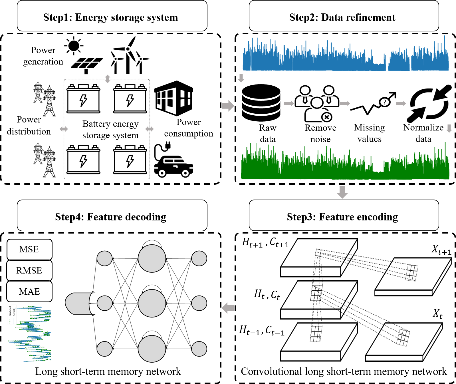
• To obtain effective forecasting results, the acquired raw data related to batteries and power consumption are first processed in a preprocessing step, where the missing values are handled using the replacement approach and normalized to expedite the model learning process.
• For battery SOH and power consumption prediction, a hybrid architecture of ConvLSTM and LSTM is presented, in which preprocessed data are passed through the ConvLSTM layers to extract spatiotemporal features in encoded form, which are then decoded by the LSTM layers for final forecasting.
• The proposed CL-Net architecture is demonstrated by a comprehensive ablation study using three distinct time series datasets and regression error metrics. The CL-Net reduces the error values up to 0.07, 0.13, and 0.135 for mean squared error (MSE), RMSE, and mean absolute error (MAE), respectively, on the NASA battery dataset. Similarly, on the IHEPC dataset, the CL-Net achieves lower values of 0.0012, 0.0052, and 0.0036 for the MSE, RMSE, and MAE, respectively, compared to the state-of-the-art. Finally, the CL-Net obtains 0.031, 0.176, and 0.169 values on the DEMS dataset for the MSE, RMSE, and MAE, respectively.

The remaining manuscript is structured in such a way that Section 2 is about the review of literature, while Section 3 provides the discussion about the proposed CL-Net architecture. Section 4 discusses the detailed experimentation while Section 5 concludes the proposed method.

2. Literature Review

Demand for the long lifetime of batteries is one of the top priorities of the manufacturers of electronic appliances as well as other electric and hybrid vehicles. For precaution purposes, battery SOH estimation can be helpful to deal with the sudden failure of BESS. However, unfortunately, battery SOH estimation is one of the difficult tasks to accurately handle. Li-ion batteries are composed of a complex mechanism that is not easy to understand. Similarly, the degradation of the batteries occurs due to several composite practices and their exchanges. This makes accurate and precise battery SOH forecasting more complicated. Dealing with these issues, different approaches are deployed to accurately predict battery SOH for the proper maintenance and replacement schedule of the batteries in systems. These techniques are categorized as experimental, model-based, and ML-based methods. A review of the different methods introduced from each of the above-mentioned approaches are listed in the sections ahead.

2.1. Experimental-Based Approaches

The experimental method is the simplest technique for understanding battery behavior. Different experiments are conducted using special equipment in order to analyze the degradation behavior of the batteries. Batteries’ internal resistance measurement is one of the experimental methods that is considered as an important factor for SOH estimation. The lifetime of the batteries can be analyzed by determining the capacity loss and the change that occurs in the internal resistance of the batteries. Several studies have investigated the experimental methods of resistance measurement. Wang et al. [17] studied the internal resistance of the batteries to control the thermal behavior of the used batteries. In another study, Wang et al. [18] analyzed the internal resistance by applying different pulse rates. Wei et al. [19] adopted the resistance measurement technique for battery life state prediction. Similarly, Remmlinger et al. [20] suggested a technique by monitoring the internal resistance of a battery in hybrid automobiles. Temperature was confirmed as a main factor for internal resistance that affects a battery life cycle. Waag et al. [21] presented different diagnostic systems that intelligently analyze a battery interior opposition throughout a life cycle. Schweiger et al. [22] determined the cell’s interior resistance by alternating current step methods and determined it as a key parameter. Chiang et al. [23] predicted battery SOH through the inner resistance with adaptive methods. They concluded that a battery’s voltage is reduced, and the internal resistance is increased when the life cycle is completed. Matsushima et al. [24] evaluated heavy storage Li-ion batteries at the industrial level and complained about the higher internal resistance in the affected batteries. In experimental methods, several studies have mentioned the measurement of the impedance value for the SOH estimation of the batteries. Electrochemical impedance spectroscopy (EIS) is a technique utilized frequently for measuring battery impedance [25]. In this procedure, the alternate current is useful, and the impedance is measured as a response of output voltage [26]. The impedance value of a battery increases as the lifetime of a battery comes closer to its end. EIS can be efficiently incorporated to predict the lifetime and SOH of batteries. Ovejas et al. [27] introduced the phenomena of Li-ion cells analysis with the help of EIS and revealed that when a battery’s lifetime is close to ending, the frequency of charge transfer is reduced. Din et al. [28] also used the concept of EIS in a real-time scenario and calculated the impedance values for a battery’s cells. In the experimental approach, Li et al. [29] conducted several experiments on Li-ion batteries and determined their SOH up to the battery’s end of life (EOL). Similarly, Xiong et al. [30] tested a battery’s capacity level and SOH at different temperatures. Another technique of ultrasonic inspection was also used for batteries’ internal health estimation [31]. Battery SOH was also analyzed using different classical destructive methods of X-ray diffractions under laboratory conditions [32]. The experimental approach of battery SOH estimation is convincing, but it has several limitations. The main limitation is that it requires a very long time period for experimentation, which is time-consuming. This approach is not applicable for online forecasting, it mainly depends on a battery’s internal chemistry and requires special laboratory equipment, so these methods are not applicable in operational conditions.

2.2. Battery Model-Based Approaches

SOH estimation is a key factor for analyzing batteries’ lifecycle and degradation level at different stages of life. Several researchers show an inclination towards model-based approaches for battery SOH estimation. Adaptive filtering such as Kalman filter (KF) is an important technique that is followed by many researchers in the literature. Koltypin et al. [33] used KF algorithm and developed an efficient and accurate battery SOH perdition model. Morigaki et al. [34] proposed an on-board SOH approach using KF to understand the internal resistance of Li-ion batteries. Plett et al. [35] used the extended KF for predicting battery SOH by calculating the cell resistance and capacity. Santhanagopalan and White [36] applied extended KF using an electrochemical cell model to estimate battery’s SOC. The results obtained using extended KF were quite accurate and the model was compatible with real-time applications. Similarly, Urbain et al. [37] measured the impedance of a battery and combined it with extended KF for the purpose of SOH estimation. Pérez et al. [38] used an enhanced extended KF approach for estimating different current profiles and states of Li-ion batteries. Their proposed model was validated over different conditions with very low error rates. The unscented KF algorithm was also used for SOH estimation, SOC estimation, and resistance measurement of Li-ion batteries [39]. Couto et al. [40] used unscented KF algorithm for analyzing battery’s cells and evaluated their model with the data from a simulator. Weihan et al. [41] developed a model-based on unscented KF for analyzing the internal states of Li-ion battery’s cells. Li et al. [35] used a dual extended KF for parameters and states estimation purposes. Next, Wang et al. [42] proposed a novel approach for the charged state prediction of Li-ion battery pack based on composite equivalent modeling and an enhanced splice KF algorithm. Researchers also gave attention to the least square-based filters (LSF) for battery SOH estimation applications. Prasad et al. [43] used LSF techniques in developing an electrochemical method to predict a battery’s SOH. Similarly, Eddahech et al. [44] used a recursive LSF algorithm for the estimation of SOC along with SOH. Todeschini et al. [45] used the LSF approach for the identification of batteries aging parameters. In other techniques, electrochemical models were used for understanding a battery’s degradation and aging behavior [46]. The fuzzy logic approach was also used for understanding the complex and nonlinear systems in battery state estimations. Salkind et al. [47] used the fuzzy logic approach along with EIS methods for predicting SOH and SOC in batteries. All these model-based approaches are commonly used in the literature of battery SOH estimation. These methods describe battery degradation phenomena with precise and accurate results up to an extent. These are relatively complex, having higher computational efforts, and require high performance controllers. The computational cost of the model-based techniques of SOH estimation is relatively high.

2.3. Machine Learning-Based Approaches

ML-based approaches use a set of measurements, observations as training data, and models for understanding a system and process for SOH estimating in batteries. ML has been widely used in BESS for the effective purpose of charge storage and battery state predictions. In the study of You et al. [15], a feedforward neural network (FNN) was used for the online SOH prediction of batteries in hybrid vehicles. Khan et al. [48] compared DL and ML techniques for Li-ion battery SOH prediction and RUL estimation. Andre et al. [49] introduced a structural architecture to predict a battery’s SOH in electric and hybrid vehicles, deducing the parameters of capacity and internal battery resistance. Chaoui et al. [50] also used FNN for SOH estimation along with time-delayed data as an input. The data of batteries such as time signals, current, and temperature were utilized to predict SOH. Furthermore, Chaoni et al. [51] used RNN for the dynamic prediction of battery SOC and SOH. Their proposed model used current, voltage, and temperature data during cycles as input parameters. In another work, You et al. [52] utilized an LSTM for battery SOH estimations in electric vehicles based on the sequential data. Veeraraghavan et al. [53] also used an LSTM network for developing a model for battery SOH estimation. Their model was trained and evaluated from the data of both real batteries and simulated data. Eddahech et al. [54] presented a hybrid approach using EIS along with an RNN based on a cell’s inner resistance and capacity. For this task, datasets were obtained performing experimentation on Li-ion batteries’ cells under aging test circumstances. Hamming neural networks along with dual extended KF were also used for predicting cells’ SOH [55]. Klass et al. [56] used a support vector machine algorithm to predict battery SOH in electric vehicles. The data were obtained from different cycle profiles of batteries at different temperatures. Saha et al. [57] used an equivalent circuit model along with particle filters and a relevance vector machine for predicting three important states of Li-ion batteries, which are RUL, SOH, and SOC. He et al. [58] applied dynamic Bayesian networks to predict battery SOH using voltage as the input attribute. SOH prediction and estimation through ML approaches show interesting and accurate results as compared to the other estimation approaches. ML approaches provide a comparatively easy implementation process with higher accuracy rates. The quality of the data provided to the ML and DL models for training and validation tasks is one of the essential aspects to be considered. Based on the above-mentioned studies, ML-based approaches are applicable for the efficient and cost-effective estimation of a battery’s SOH in ESS, electronic and hybrid vehicles, and other electronic appliances.

3. Proposed Method

This section thoroughly explains the overall steps held in the SOH and power consumption forecasting mechanism with visual representation. Initially, data from the acquisition step are preprocessed for the removal of noise and handling missing values, and then its normalization is performed. The refined data are passed into the proposed CL-Net architecture, which is a hybrid connection of two networks including ConvLSTM and LSTM as shown in Figure 1. The initial ConvLSTM layers extract the most discriminative and hierarchical features from the input sequence that are forward propagated into the LSTM network. The latter features obtained from the LSTM network are passed into other fully connected layers that give final forecasting results. The applied several sequential approaches will be covered in the subsequent sections.

3.1. Data Acquisition and Refinement

Energy demand is increased as population of the world rises, due to which the quantity of carbon dioxide also increases. RESs can protect the world from climate change and provide a human friendly environment. Sustainable energy can be provided by RESs, which are endless and never run out, such as wind and solar energies. There are some challenges in renewable energy such as these resources of power are uncontrollable by humans. Wind energy is available when wind is blowing while solar energy is dependent on the sunshine. To tackle the above-mentioned problems, BESS is used where energy is stored for a high demand duration or when the power is not available from RESs. To make BESS safe from any damage, SOH forecasting of a battery is a very important task. There are various smart meters for energy consumption measurement and battery-related attributes such as temperature, current, and voltage. The raw data obtained from these smart meters have different types of issues such as missing values, noise, data redundancy, and outliers. Therefore, preprocessing is a main step in time series problems where the data are cleaned and made suitable for model training. During the collection of raw data, missing values and outliers can occur due to human behavior and environmental conditions. ML and DL models decrease their performance for time series problems if the data have missing values and outliers [59]. Therefore, a substitution method is used for filling the missing values where a previous value at that time is used to fill the current missing values. Similarly, outliers in a dataset are the values deviated from the remaining data, due to which models for time series data are less accurate and their predictions are corrupted. Thus, to remove outliers and noise from the raw data, moving average filter method is employed where the data are made smooth for training the model. Data normalization is a very important step in data preparation for DL models where raw data values are scaled to a particular range. Therefore, the normalization process of min-max is applied to scale the input sequence values in a range from 0 to 1, where the difference between the values is not distorted. The raw data are normalized using Equation (1), where $\overline{x}$ is normalized data, $x$ is unscaled data, while $min$ and $max$ are minimum and maximum values in the input dataset:

$$\overline{x}=\frac{\left(x-min\right)}{max-min}$$

(1)

3.2. Sequential Networks

This section is about the proposed approach for SOH forecasting of batteries and power consumption. LSTM is used separately and with various other DL models as a hybrid network for forecasting. The proposed architecture and other hybrid models are discussed in the following subsections.

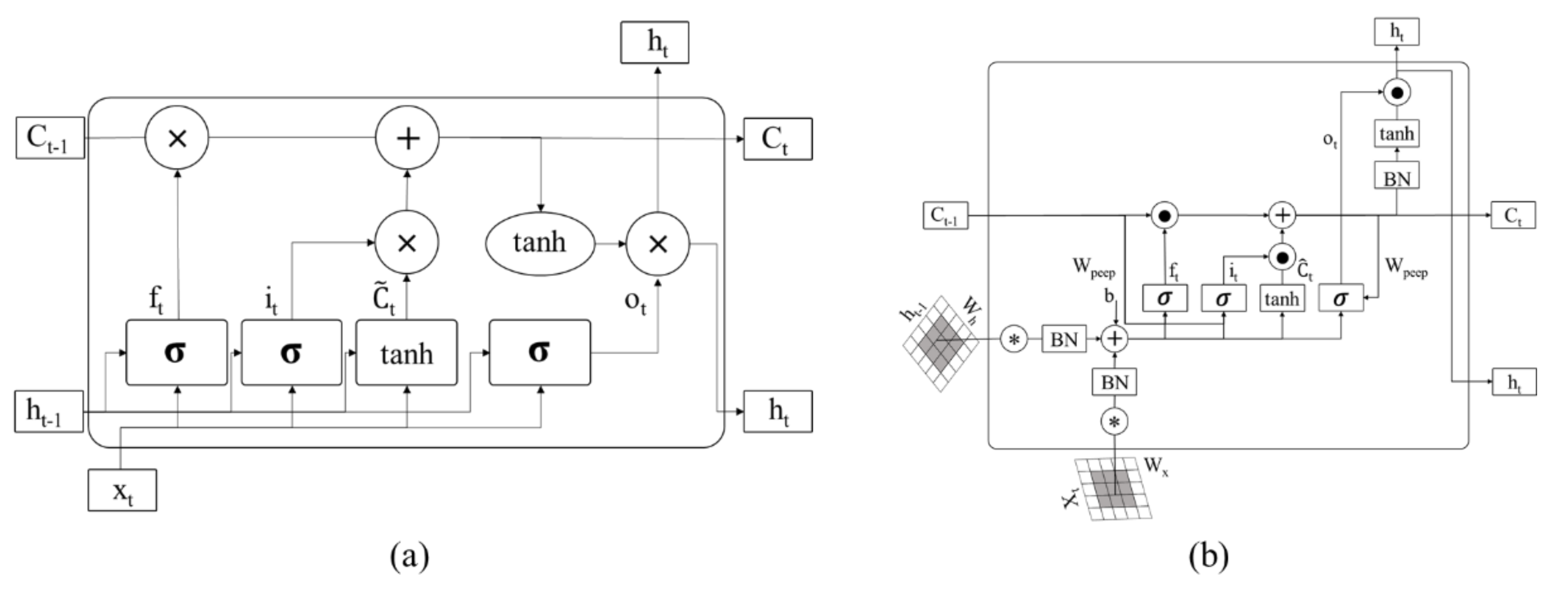
3.2.1. Long Short-Term Memory Network

Recent advancements in huge data availability and DL techniques have made the time series data-driven prediction more prestigious and affordable including forecasting and vision-related tasks such as crowd analysis [60]. However, the established literature on LSTM for time series problems gives an important direction for SOH estimation of batteries as well as power consumption. LSTM networks are a type of RNN that are widely famous for processing the sequential data and addressing the long-term memory drawbacks of vanilla RNN. LSTM extends the architecture of RNN using a gating mechanism and a standalone memory cell, which regulates the flow of information throughout the network. The gating concept comprises of three units, such as input, forgot, and output gate. These gates control the flow of information across the network to allow which information needs to persist or how long it will persist after reading it from the cell memory. LSTM networks are capable to retain the key information and discard the less important information. The memory cell has a recurrent self-connected unit known as constant error carousel (CEC) that has a state vector to preserve long-term dependencies. Next, to distinguish self-contained cell memory from conventional state $h_t$ in LSTM, it is referred as $c_t$. The forget gate $f_t$ obtains input $x_t$ and $h_{t-1}$ to determine which information needs to be retained in $c_{t-1}.$ The activation functions for gates $i_t, o_t,$ and $f_t$ are sigmoid layers where each value is projected between 0 and 1 while $c_{t-1}$ gives the information retention to describe the scale. Further details are beyond the scope of the paper. However, the aforementioned process is formally defined through Equation (2) to Equation (6), and Figure 2a illustrates the cell architecture of LSTM network:

$$i_t=\sigma \left(W_{xi}{x}_t+W_{hi}{h}_{t-1}+W_{ci}○c_{t-1}+b_i\right)$$

(2)

$$f_t=\sigma \left(W_{xf}{x}_t+W_{hf}{h}_{t-1}+W_{cf}○c_{t-1}+b_f\right)$$

(3)

$$o_t=\sigma \left(W_{xo}{x}_t+W_{ho}{h}_{t-1}+W_{co}○c_t+b_0\right)$$

(4)

$$c_t=f_t○c_{t-1}+i_t○\varnothing \left(W_{xc}{x}_t+W_{hc}{h}_{t-1}+b_c\right)$$

(5)

$$h_t=o_t○\varnothing \left(c_t\right)$$

(6)

Here, $W_{xi}$,$W_{hi}$,$W_{ci}$,$W_{xf}$,$W_{hf}$,$W_{cf}$ $W_{xo}$,$W_{ho}$,$W_{co}$, $W_{xc}$, and$W_{hc}$ indicate weight matrices for the gates and cell memory state, while $h_{t-1}$ is a previous hidden state, and $c_t$ is a cell state. The biases of the gates are represented through $b_i$, $b_o$, $b_f$, and $b_c$ while $○$ indicating an element-wise multiplication procedure. Similarly, $\sigma$ shows the logistic sigmoid function, and $\varnothing$ represents hyperbolic tangent function. These activation functions are defined separately in Equations (7) and (8):

$$\sigma \left(x\right)=\frac{1}{1+e^{-x}}$$

(7)

$$\varnothing \left(x\right)=\frac{e^x-e^{-x}}{e^x+e^{-x}}$$

(8)

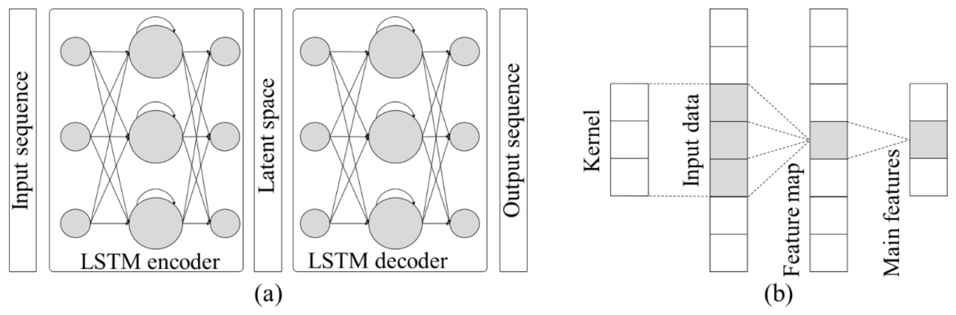
3.2.2. Encoder–Decoder Network

In time series data, problems can be classification or regression problems, where, in classification, the output of a model is a label, while in regression, it is a continuous value. Regression problems can be single- or multi-step, where, in single-step, the output is one next value, while in multi-step, the output has multiple next values. There are other types of regression problems, but one of them is known as a sequence-to-sequence prediction problem, which is a more challenging task in this domain. In this problem, the input data to a model are sequential, while the output of the model is also a sequence instead of predicting a single value for the given input. So, the more efficient and proven to be an effective approach for sequence-to-sequence problems is encoder–decoder. There are two further networks in this approach, where the first network reads the input sequence and converts it into a fixed-length vector in encoded form while the second network decodes the fixed-length vector by given output as a predicted sequence. These architectures are specifically designed for sequence-to-sequence problems and are called encoder–decoder, as shown in Figure 3a. For the purpose of SOH and power consumption forecasting, the input sequence is passed through an encoder to encode the important information from the input sequence. After the encoding mechanism, the encoded features are decoded via plugging an additional unit known as the decoder. The latter generated from the decoder is propagated to fully connected layers that give the final sequence prediction of the input sequence.

3.2.3. CNN and LSTM Hybrid Network

This section discusses about the hybrid connection of CNN and LSTM networks known as CNN-LSTM. The hybrid connection is the prediction model that obtains univariate time series data and gives multi-step forecasting. CNN is a DL-based algorithm that considers spatial inputs and is identical to other neural networks with neurons, learnable weights and biases in them. CNN acts as FNN, where the flow of information happens in one direction, i.e., input to their outputs, as shown in Figure 3b. In the proposed work, the hybrid connection of CNN-LSTM comprises of CNN layers and the LSTM network. The CNN layers extract the features from the time series variables that are given to LSTM to assist the prediction process. In the hybrid connection, 1D CNN is used, where each convolutional layer is followed by a max pooling layer, and its output is flattened and fed into the LSTM units. LSTM layers are followed by dense or fully connected layers to give a final prediction. Initially, the data are rescaled and reshaped to fit the three-dimensional input. The input time steps are defined as various leg values with one feature for the univariate model. Overfitting is one of the main issues common in deep neural networks. There are several solutions, and the dropout is one of the simplest and most efficient that works well. To avoid overfitting, a dropout layer is plugged, whose output is next provided to fully connected layers. Next, there are several frequently used activation functions such as sigmoid function, ReLU function, and tanh function. In these functions, the ReLU function solves the gradient disappearance problem. Next, its calculation and convergence speeds are faster than tanh and sigmoid functions. The working process of the ReLU function is defined in Equation (9). The output of a convolution process is represented in Equation (10) and Equation (11), where $f$ is the input sequence, $h$ is a filter, while $m$ and $n$ are the data dimensions:

$$Ҩ\left(x\right)=\max \left(0,x\right)$$

(9)

$$G\left[m,n\right]=\left(f\ast h\right)\left[m, n\right]$$

(10)

$$\left(f\ast h\right)\left[m, n\right]={{\displaystyle \sum }}_j{{\displaystyle \sum }}_{k}h\left[j,k\right]f\left[m-j,n-k\right]$$

(11)

3.2.4. Convolutional LSTM and LSTM Hybrid Network

Learning via fully connected layers of LSTM has been proven to be powerful to handle temporal correlation; however, a lot of redundancy from spatial data has made it more challenging. To handle this issue, the fully connected LSTM has added an extension having convolutional assembly in both state-to-state and input-to-state transitions. Stacking multiple layers of ConvLSTM by forming encoding and forecasting mechanisms have made the network not only capable of precipitation new casting but also for spatiotemporal forecasting. Similar to the conventional fully connected LSTM, ConvLSTM is also adopted as a building block to handle more complex sequences. Figure 2b illustrates the cell architecture of ConvLSTM. These layers act as an encoder that encodes the input-refined sequence having a defined size, which is then forward propagated into LSTM. ConvLSTM applies convolution operations for the input to hidden and hidden to hidden connection. To replace matrix multiplication operations in RNN, ConvLSTM layers with convolution operations are used, and these layers have the ability to know which information needs to be remembered or to be forgotten from the previous cell state via the forget gate [61]. Similarly, ConvLSTM decides which information will be stored in the current cell. The process of ConvLSTM is described in Equation (12) to Equation (16). After ConvLSTM, an additional LSTM layer is plugged that learns the features map and gives the final prediction. Making this hybrid connection is more efficient and effective in term of correct battery SOH and power consumption forecasting:

$$i_t=\sigma \left(W_{xi}\ast x_t+W_{hi}\ast h_{t-1}+W_{ci}\circ c_{t-1}+b_i\right)$$

(12)

$$f_t=\sigma \left(W_{xf}\ast x_t+W_{hf}\ast h_{t-1}+W_{cf}\circ c_{t-1}+b_f\right)$$

(13)

$$o_t=\sigma \left(W_{xo}\ast x_t+W_{ho}\ast h_{t-1}+W_{co}\circ c_t+b_o\right)$$

(14)

$$c_t=f_t○c_{t-1}+i_t○\varnothing \left(W_{xc}\ast x_t+W_{hc}\ast h_{t-1}+b_c\right)$$

(15)

$$h_t=o_t○\varnothing \left(c_t\right)$$

(16)

4. Experimental Results

This section mainly discusses the datasets, the experimental results, the empirical analysis of the outcome in terms of useful metrics, and a comparative study. These topics are covered in the following subsections.

4.1. System Configuration and Implementation Details

The proposed architecture is implemented in Python language (Version 3.8.5) using the most popular DL framework Keras (Version 2.5.0) with TensorFlow (Version 2.5.0) at the backend. The hardware setup consists of a Windows 10 operating system with an AMD Ryzen 9 3900X 12-core processor, NVIDIA graphics processing unit (GeForce RTX 3090), and 48.0 GB installed RAM. To confirm and validate the efficiency of the different sequential models, three different time series datasets are used, including NASA battery [62], IHEPC [63], and DEMS, which are collected from the prognostic data repository, the UCI ML repository, and the Korean local energy management system, respectively. Next, the model’s validation is performed using the hold-out method where the data are divided into training and testing parts. In this study, 70% of each dataset is used as training and 30% for testing purposes. Furthermore, each model is trained with a batch size of 16, Adam optimizer, and 100 epochs.

4.2. Datasets

In this study, three different time series challenging datasets are utilized to conduct the ablation study on the various sequential models. The following subsections discuss these datasets in detail.

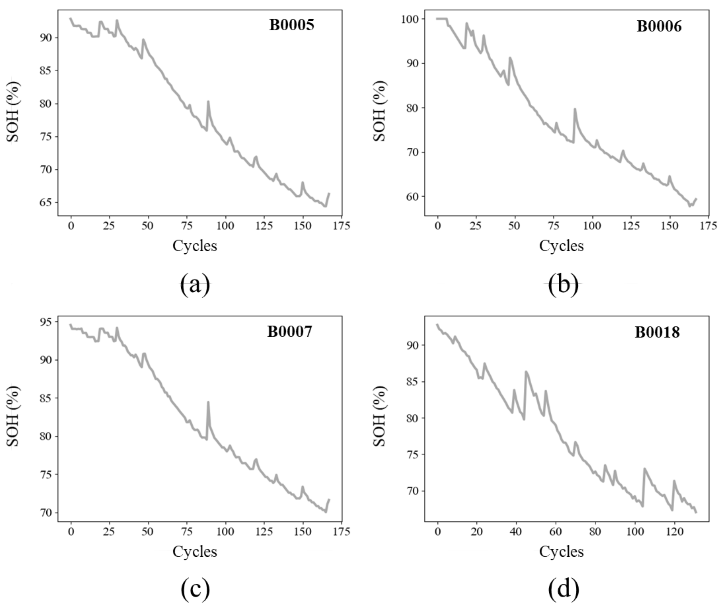
4.2.1. NASA Battery Dataset

This dataset is produced by the prognostics center of excellence at NASA Ames using Li-ion batteries [62] and is considered as a benchmark in batteries-related research. It has been widely used for battery capacity, SOH, RUL, and SOC estimations. Four batteries, including B0018, B0007, B0006, and B0005, were used in the experiments by performing different operations such as charging, impedance, and discharging at room temperature to analyze them. All the batteries were charged at 1.5 amperes until their voltage reached 4.2 volts. At 4.2 volts, the voltage was kept constant and the current was reduced to 20 milli-amperes during charging. Similarly, during discharging, the current was kept constant at 2 amperes, and the voltages were dropped to 2.5, 2.2, 2.5, and 2.7 volts for batteries B0018, B0007, B0006, and B0005, respectively. The process of charging and discharging was carried on for all the batteries until they reached their EOL. The EOL was defined by the research center, which was the reduction of 30% in the rated capacity of a battery. The SOH of a battery can be calculated using Equation (17), where $C_m$ is the maximum capacity while $C_r$ is the rated capacity of the battery. The degradation in the SOH of each battery according to a number of cycles is shown in Figure 4.

$$SOH=\frac{C_m}{C_r}100\%$$

(17)

4.2.2. Individual Household Electric Power Consumption Dataset

This dataset is obtained from the UCI repository [63] that consists of data measured from a house located in Sceaux, France in the period of 2006 to 2010, making 47 months of total power data. There are a total of 2,075,259 samples, where 25,941 contain missing values and is 1.25% of the total data. The issue of these missing values is resolved in the preprocessing step. The basic time resolution used in this dataset is minutely horizon. The power is consumed over every minute and is given in kilowatts. Different time resolutions can be formed such as hours, days, and weeks where a data sequence is given to the network. Some samples of the data are shown in Figure 5a while

Table 1. IHEPC dataset attributes and their description.

Attributes	Description
Date	This variable represents the date when the data was recorded. The date is comprised of years, months, and days.
Time	This variable contains the values measured in hours, minutes, and seconds where the row-to-row jump is one minute.
Global active power	This attribute shows the overall active power consumed by the appliances and is represented by the GAP. The GAP is measured in kilowatts.
Global reactive power	This attribute shows the overall reactive power, and its symbol is GRP. The GRP is also measured in kilowatts.
Voltage	This attribute is measured in volts and is represented by V.
Global intensity	This variable shows the overall intensity of the current and is represented by GI. The GI is measured in amperes.
Sub_metering_S1	The power energy consumed by the devices in the kitchen such as microwave, dishwasher, etc. It is measured in watt-hour.
Sub_metering_S2	The power energy consumed by the machineries in the laundry room such as refrigerator and washing machine, and is measured in watt-hour.
Sub_metering_S3	The power energy consumed by the water cooler and air-conditioner, and it is also measured in watt-hour.

describes the attributes used in this dataset with their remarks.

4.2.3. Domestic Energy Management System Dataset

This dataset is collected from local Korean ESS batteries in the period of 21 March 2017 to 24 September 2019. The dataset consists of three batteries, including BAT1, BAT2, and BAT3, where each battery’s data are originally structured in the resolution of seconds. BAT1 contains 38,733,091 total instances having multi-variate data while BAT2 and BAT3 have 38,732,890 and 38,731,915 instances, respectively. Different time resolutions of the batteries’ data can be made such as minutes, hours, and days where a lag sequence is given to the model for forecasting. In the DEMS dataset, each battery has 78 different attributes at the rack and battery levels such as date-time, temperature, SOC, voltage, current, and SOH, etc. In this study, the hourly resolution of the data is chosen and the SOH attribute for all three batteries is forecasted. Some samples of the DEMS dataset in hourly resolution are depicted in Figure 5b.

4.3. Evaluation Metrics

It is an essential step to evaluate the proposed approach using different metrics that helps to verify the effectiveness of the work. In the literature, several metrics are used depending on the particular problem such as accuracy, recall, precision, etc., which are abundantly used for classification purposes. However, the forecasting time series data is a regression problem, therefore, to confirm its effectiveness, the MSE, RMSE, and MAE error metrics are used. MSE is the average square of difference between the actual and predicted values, while RMSE is the square root of the MSE. Next, the MAE represents the average absolute difference in the actual and predicted values. These metrics are well presented in Equation (18) to Equation (20):

$$\mathrm{MSE}=\frac{1}{n}{{\displaystyle \sum }}_1^n{\left(y-ŷ\right)}^2$$

(18)

$$\mathrm{RMSE}=\sqrt{\frac{1}{n}{{\displaystyle \sum }}_1^n{\left(y-ŷ\right)}^2}$$

(19)

$$\mathrm{MAE}=\frac{1}{n}{{\displaystyle \sum }}_1^n\left|y-ŷ\right|$$

(20)

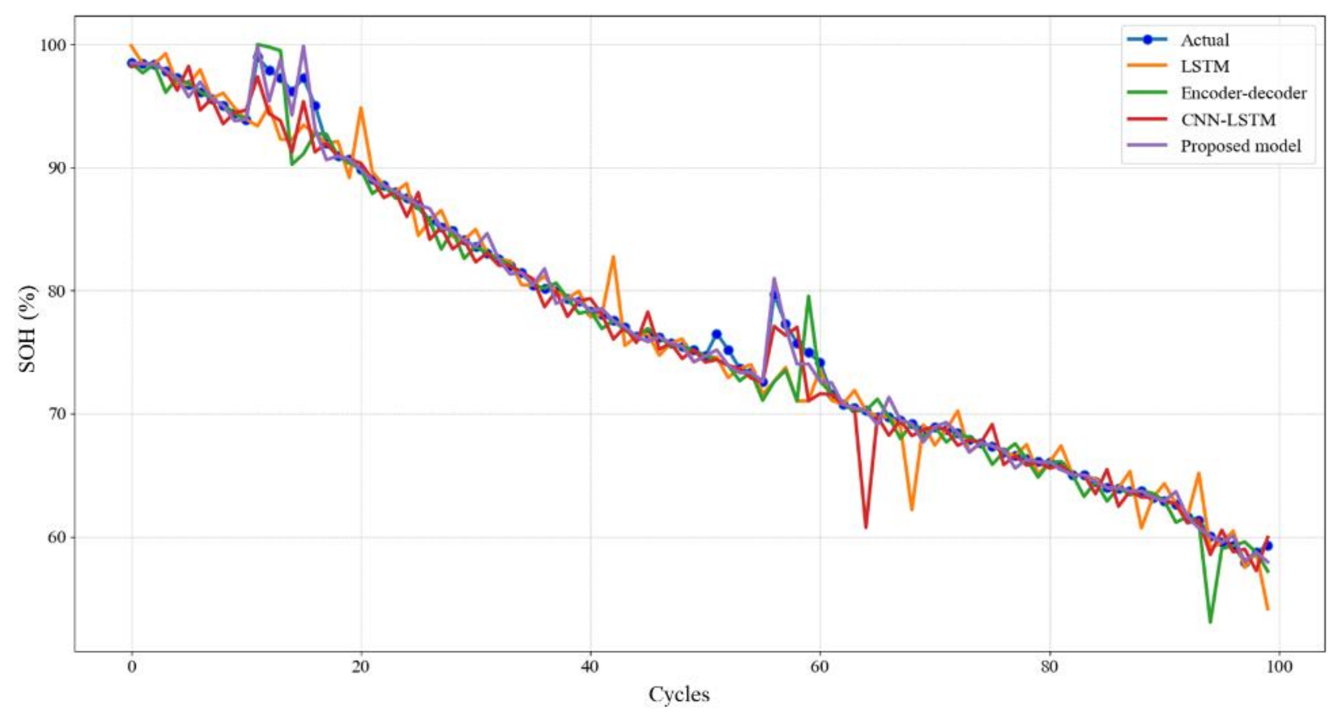
4.4. Ablation Study on the NASA Battery Dataset

The overall results obtained on the NASA battery dataset are discussed in this section. Method evaluation is performed on the NASA battery data using different sequential learning algorithms. The NASA battery dataset is comprised of four Li-ion batteries where each one having different number of cycles. The dataset is firstly tested by LSTM to identify and forecast the SOH. The performance of LSTM can be observed from the metrics where values for the MSE, RMSE, MAE of the LSTM network are 0.067, 0.259, and 0.209, respectively. LSTM utilizes the input sequence from the SOH attributes and extracts meaningful information from it. Further assessment is performed via an encoder–decoder network to identify its performance on the NASA data, and its results are given in

Table 2. Forecasting results obtained on the NASA battery dataset using different sequential models.

Method	MSE	RMSE	MAE
LSTM	0.067	0.259	0.209
Encoder–decoder	0.049	0.221	0.172
CNN-LSTM	0.061	0.247	0.195
Proposed method	0.042	0.205	0.151

. Similarly, the CNN and LSTM-based hybrid connection network is also studied to explore its use for SOH forecasting. The MSE, RMSE, and MAE values obtained by the CNN-LSTM are 0.061, 0.247, and 0.195, respectively. Finally, the results obtained on the proposed CL-Net architecture are discussed, where the MSE, RMSE, and MAE values are 0.042, 0.205, and 0.151, respectively. Figure 6 shows the visual results of the different sequential methods on the NASA battery dataset while the overall performance results are posted in Table 2.

4.5. Ablation Study on the IHEPC Dataset

The numerical results obtained on the IHEPC dataset using hourly resolution are given in

Table 3. Results obtained on the IHEPC dataset in hourly resolution for a day ahead prediction using different sequential models.

Method	MSE	RMSE	MAE
LSTM	0.027	0.164	0.099
Encoder–decoder	0.019	0.137	0.091
CNN-LSTM	0.021	0.145	0.092
Proposed method	0.015	0.122	0.088

while the visual prediction results of the sequential models are depicted in Figure 7. At first, experiments on the LSTM are performed to check and confirm its performance. LSTM is a type of RNN that is trained via backpropagation through time approach to overcome the problem of vanishing gradients. The layers used in the LSTM are kept with the default settings where the memory blocks are connected using layers. These blocks contain some components which make them smarter than a single neuron. The block has gates that manage its output and state. A single block operates an input sequence where each gate uses the sigmoid activation unit. Each unit acts as a mini-state machine having weights, which are learned in training process. After training the LSTM on the IHEPC dataset, the obtained MSE, RMSE, and MAE on an hourly horizon are 0.027, 0.164, and 0.099, respectively. After LSTM, encoder–decoder is applied, which is the hybrid connection of the LSTM encoder and decoder. The initial part involves the LSTM, where it first encodes the given sequence while the second part decodes it. The encoder consists of few recurrent units, which accept a single input sequence that collects the important information and forward propagates it. The encoder part produces an encoded vector, which is the final state that comes from the encoder part. After encoding, the latter from the encoder part is fed into the decoder. The prediction is obtained from the decoder part, and a fully connected layer is added that performs the final prediction process. The MSE, RMSE, and MAE of the encoder–decoder are 0.019, 0.137, and 0.091, respectively. Furthermore, the performance of the hybrid connection of CNN and LSTM is also evaluated, which is abundantly used in several forecasting tasks. CNN-LSTM consists of CNN and LSTM layers where CNN extracts the most discriminative and important features from the input sequence that are given to the LSTM to learn them for the final prediction. The main advantage of using CNNs is the usage of convolutions or filters, which make them capable of power consumption forecasting. The space size in the cell allows the network to better examine the observation in series. Therefore, the CNN and LSTM layers combined in the forecasting problem allow the LSTM to encounter long-term dependencies in the series. In this case, the LSTM gives the final forecasting for power consumption. The obtained results on CNN-LSTM are such that the MSE, RMSE, and MAE values are 0.021, 0.145, and 0.092, respectively. After CNN-LSTM, the results obtained from the proposed method are compared, which is the connection of a ConvLSTM and a simple LSTM network in a hybrid way. Unlike the simple LSTM or CNN-LSTM that calculates the internal state and interprets the output from CNN, the ConvLSTM uses convolutions directly by reading the input into the LSTM. However, the proposed method adds additional LSTM layers to ConvLSTM layers to make their strong hybrid connection. The MSE, RMSE, and MAE using the proposed method are 0.015, 0.122, and 0.088, respectively.

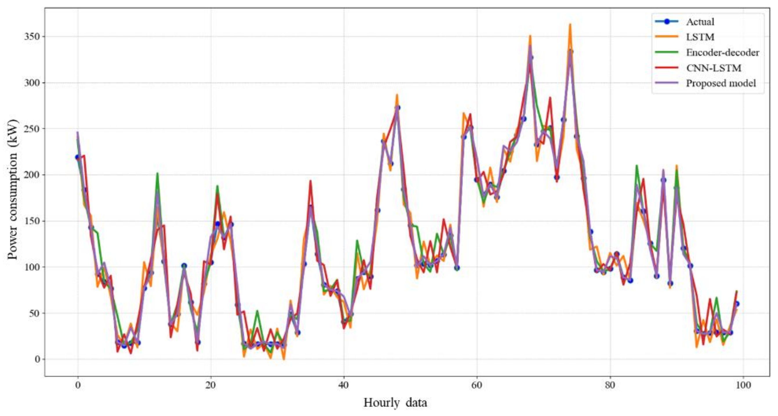
4.6. Ablation Study on the DEMS Dataset

This section discusses the overall results obtained on the DEMS dataset. Similar to the previous dataset, the sequential learning techniques are also investigated for the DEMS dataset. At first, the LSTM network is practiced for its performance on the DEMS batteries data where each sequential model has been applied to hourly horizon of the dataset. The values for the MSE, RMSE, MAE of the LSTM network for hourly horizon are 0.045, 0.212, and 0.194, respectively. The overall results are given in

Table 4. Results obtained on the DEMS dataset in hourly resolution for a day ahead forecasting using different sequential models.

Method	MSE	RMSE	MAE
LSTM	0.045	0.212	0.194
Encoder–decoder	0.036	0.190	0.173
CNN-LSTM	0.039	0.197	0.179
Proposed method	0.031	0.176	0.169

. For the LSTM network, the default settings are used that are applied on the previous dataset. LSTM obtains the sequence of input variables from the SOH attribute and extracts the important information from it. Similarly, the encoder–decoder network is also analyzed to forecast the SOH of the batteries. The setting parameters are the same that are applied on the NASA and IHEPC datasets in the previous subsections. However, if the results obtained on the DEMS batteries data are analyzed as compared to LSTM, they are improved. The results obtained from the encoder–decoder are given in Table 4, where the MSE, RMSE, MAE values are 0.036, 0.190, and 0.173, respectively. Next, the hybrid connection of CNN and LSTM is explored, which is previously explained in detail. The MSE, RMSE, and MAE values obtained from the CNN-LSTM are 0.039, 0.197, and 0.179, respectively. Finally, the results obtained from the proposed method are discussed that are also given in Table 4. The obtained MSE, RMSE, and MAE values of the CL-Net are 0.031, 0.176, and 0.169, respectively. Figure 8 shows visual results of the different sequential methods on the hourly resolution data.

4.7. Comparative Analysis Using the NASA Battery Dataset

This section discusses the comparative analysis of the proposed architecture with other works in the literature using the NASA battery dataset. For instance, a Gaussian process regression method [11] is proposed for a battery’s SOH estimation based on partial incremental capacity curve. In this method, smoothing incremental capacity curves are obtained using Gaussian filters, and then health indices are extracted as the input features. To predict the SOH of a battery, mean and covariance functions are applied where the average values of 1.030, 1.015, and 0.387 are obtained for MSE, RMSE, and MAE, respectively. Next, wavelet neural networks with a genetic algorithm [9] are compared for battery SOH prediction using an incremental capacity mechanism. This method first extracts important features from incremental capacity curves through Pearson’s correlation coefficient approach. To optimize the wavelet neural networks scaling factor, translation factor, and initial connection weights, a genetic algorithm is used. To predict the SOH of a battery, a genetic algorithm with wavelet neural networks is utilized. Different models are used in this study, but the genetic algorithm with wavelet neural network shows the best performance by obtaining an average MAE value of 1.655 on the NASA battery data. Similarly, a parallel layer extreme learning machine algorithm [12] is proposed to enhance the battery’s SOH. They compared two methods where the parallel layer extreme learning machine algorithm shows high performance by obtaining the MSE, RMSE, and MAE values of 0.112, 0.335, and 0.286, respectively. Finally, the proposed CL-Net architecture obtains 0.042, 0.205, and 0.151 values for MSE, RMSE, and MAE, respectively, which prove that the proposed approach outperforms the state-of-the-arts in terms of error metrics. The detailed comparative results are presented in

Table 5. Proposed method comparison with state-of-the-art methods using the NASA battery dataset.

Ref	Method	MSE	RMSE	MAE
[11]	Gaussian process regression	1.030	1.015	0.387
[9]	GA-WNN	---	---	1.655
	WNN	---	---	3.320
	BP	---	---	7.530
	SVM	---	---	4.697
[12]	PL-ELM	0.112	0.335	0.286
	ELM	1.124	1.060	0.676
Proposed method		0.042	0.205	0.151

.

4.8. Comparative Analysis Using the IHEPC Dataset

This section thoroughly explains the comparative analysis of the proposed architecture with other competitive state-of-art methods. The comparison is performed for the results obtained on hourly resolution using the IHEPC dataset. First, the sequence-to-sequence (seq2seq) [64] method is studied and analyzed for its consumption nature, which investigated two types of LSTM architectures, including standard LSTM and LSTM-based seq2seq architectures. This method shows that the LSTM performed better on hourly resolution while it fails on minutely resolution. The obtained RMSE on their method is 0.625. Next, the CNN-LSTM [65] is explored, which is the hybrid connection of the CNN and LSTM networks where CNN extracts the complex features from the consumption variables that effect the consumption. LSTM, in their network, is responsible for modeling the temporal information. The MSE, RMSE, MAE values achieved by the CNN-LSTM are 0.3549, 0.5957, and 0.3317, respectively. Similarly, another method [66] introduced an explainable autoencoder to predict the consumption for 15, 30, 45, and 60 min. They used a t-SNE algorithm to visualize and explain the prediction results. Their method gave values of 0.3840 and 0.3953 for the MSE and MAE, respectively. Furthermore, the most recently published work in the reference [67] is compared, which introduced the DB-Net architecture to predict energy consumption using the hybrid connection of dilated CNN and bidirectional LSTM networks. The MSE, RMSE, and MAE obtained by this method are 0.0162, 0.0112, and 0.0916, respectively. Next, in [68], a comprehensive study is conducted on the traditional ML algorithms and DL sequential models for load consumption prediction. Their comparison found that the multilayer LSTM (M-LSTM) showed the highest performance as compared to the traditional ML and DL algorithms in terms of the error metrics. On the hourly resolution data, the M-LSTM obtained values of 0.1087, 0.3296, and 0.3086 for MSE, RMSE, and MAE, respectively. Similarly, the study [69] introduced a novel hybrid DL-based sequential model for commercial and residential sectors load consumption forecasting where the model obtained values of 0.105, 0.324, and 0.311 for MSE, RMSE, and MAE, respectively. In addition, an RNN model with multi-headed attention is introduced in [70] to learn spatiotemporal features selectively and predict power consumption, where the model obtained a value of 0.2662 for MSE. Similarly, in [71], a hybrid network based on dilated convolutions and residual gated recurrent units (RGRU) is proposed for forecasting power consumption and generation by obtaining values of 0.17, 0.41, and 0.26 for MSE, RMSE, and MAE, respectively. Finally, the proposed architecture obtains values of 0.015, 0.122, and 0.088 for MSE, RMSE, and MAE, respectively, which proves that the CL-Net architecture outperforms the state-of-the-arts in terms of error metrics. These comparison results are presented in

Table 6. Comparison with state-of-the-art methods using the IHEPC hourly resolution dataset.

Ref	Method	MSE	RMSE	MAE
[64]	Seq2Seq	---	0.625	---
[65]	CNN-LSTM	0.3549	0.5957	0.3317
[66]	Explainable autoencoder	0.3840	---	0.3953
[67]	DB-Net	0.0162	0.1272	0.0916
[68]	M-LSTM	0.1087	0.3296	0.3086
[69]	Hybrid DL netwok	0.105	0.324	0.311
[70]	Multi-headed attention model	0.2662	---	---
[71]	RGRU-based hybrid model	0.17	0.41	0.26
Proposed method		0.015	0.122	0.088

.

4.9. Time Complexity Analysis of the Sequential Models

In this section, an ablation study is conducted for the battery SOH and power consumption forecasting using four different sequential models, including LSTM, encoder–decoder, CNN-LSTM, and CL-Net, which is the proposed hybrid architecture of the ConvLSTM and LSTM. All four models are validated using regression error metrics on the time series datasets, including NASA battery, IHEPC, and DEMS, where the proposed CL-Net architecture obtains the lowest error rate as compared to the other models. Next, the model inference time is an important factor for real-time scenarios. Therefore, the time complexity of all the four models in terms of their training and testing time using all the datasets is compared. For the experimentation, a hardware system with an AMD Ryzen 9 3900X 12-core processor, NVIDIA graphics processing unit (GeForce RTX 3090), 48.0 GB RAM, and installed Window 10 operating system is used. All the datasets are divided into 70% and 30% training and testing sets, respectively. The training time of the proposed architecture on the NASA battery dataset for one epoch is 3.05 s, while the testing time on the same dataset is 0.41 s. Next, on the IHEPC hourly resolution data the proposed CL-Net architecture training time is 51.88 s for a single epoch while its testing time is 13.74 s. Similarly, using the hourly resolution of the DEMS dataset, the training time for one epoch taken by the proposed architecture is 87.37 s, while the testing time on the same dataset is 26.55 s. The training and testing time of all four models on the three datasets are given in

Table 7. Time complexity analysis of the proposed architecture and other sequential models in seconds (s) on the NASA battery, IHEPC, and DEMS datasets.

Method	NASA Dataset		IHEPC Dataset		DEMS Dataset
	Training Time (s)	Testing Time (s)	Training Time (s)	Testing Time (s)	Training Time (s)	Testing Time (s)
LSTM	3.18	0.45	87.16	13.96	146.22	30.58
Encoder–decoder	5.61	0.69	225.22	16.77	405.18	33.80
CNN-LSTM	3.36	0.57	126.03	14.23	222.28	28.57
Proposed method	3.05	0.41	51.88	13.74	87.37	26.55

, where the proposed architecture requires a small amount of time for training and testing as compared to the others sequential models.

5. Conclusions

SOH plays an important role in ESS by analyzing and estimating batteries in order to decrease the high risk of accidents and failure. It is also required to extend batteries’ lifespans. Similarly, precise power consumption forecasting is also necessary to minimize energy shortage and oversupply. Thus, to improve battery performance by SOH estimation and demand-side management, this paper proposed a novel hybrid architecture named CL-Net by integrating the ConvLSTM and LSTM for multi-step SOH and power consumption forecasting. Initially, the collected raw data from smart meters are passed into the refinement layer to clean them from noise and abnormalities. The refined data are then fed to the ConvLSTM layers that extract spatiotemporal features by encoding them. Next, an additional set of LSTM layers are attached that decode the resultant output from the ConvLSTM layers, followed by a fully connected layer for the final forecasting of a battery’s SOH and power consumption. To verify and evaluate the effectiveness of the proposed architecture, three datasets were used, such as the NASA battery, IHEPC, and DEMS datasets. The comparative study shows that the proposed architecture is effective and efficient for multi-step battery SOH as well as power consumption forecasting. The proposed architecture obtains values of 0.042, 0.205, 0.151 for the MSE, RMSE, and MAE, respectively, on the NASA battery data. Similarly, on the IHEPC dataset, the architecture obtains values of 0.015, 0.122, and 0.088 for the MSE, RMSE, and MAE respectively. Finally, the CL-Net obtains values of 0.031, 0.176, 0.169 on the DEMS dataset for the MSE, RMSE, and MAE, respectively. Furthermore, the influence of a battery’s temperature on SOH and weather-related variables’ impact on power consumption is not considered in this work, therefore, the approach might be improved by including this information.

In the future, it is aimed to further analyze additional parameters to forecast SOH, power consumption and generation by considering real-world data that include environmental aspects and weather-related attributes. It is also intended to include an edge computing module for long-term battery SOH, power consumption, and generation forecasting to reduce costs and energy.

References

1. Khan, N.; Ullah, F.U.M.; Haq, I.U.; Khan, S.U.; Lee, M.Y.; Baik, S.W. AB-Net: A Novel Deep Learning Assisted Framework for Renewable Energy Generation Forecasting. Mathematics 2021, 9, 2456. [Google Scholar] [CrossRef]
2. Li, Y.; Zhong, S.; Zhong, Q.; Shi, K. Lithium-ion battery state of health monitoring based on ensemble learning. IEEE Access 2019, 7, 8754–8762. [Google Scholar] [CrossRef]
3. Han, X.; Ouyang, M.; Lu, L.; Li, J.; Zheng, Y.; Li, Z. A comparative study of commercial lithium ion battery cycle life in electrical vehicle: Aging mechanism identification. J. Power Sources 2014, 251, 38–54. [Google Scholar] [CrossRef]
4. Fan, Y.; Xiao, F.; Li, C.; Yang, G.; Tang, X. A novel deep learning framework for state of health estimation of lithium-ion battery. J. Energy Storage 2020, 32, 101741. [Google Scholar] [CrossRef]
5. Wu, Y.; Xue, Q.; Shen, J.; Lei, Z.; Chen, Z.; Liu, Y. State of health estimation for lithium-ion batteries based on healthy features and long short-term memory. IEEE Access 2020, 8, 28533–28547. [Google Scholar] [CrossRef]
6. Galeotti, M.; Giammanco, C.; Cinà, L.; Cordiner, S.; Carlo, A.D. Synthetic methods for the evaluation of the State of Health (SOH) of nickel-metal hydride (NiMH) batteries. Energy Convers. Manag. 2015, 92, 1–9. [Google Scholar] [CrossRef]
7. Chen, Z.; Weng, C.; He, X.; Han, X.; Lu, L.; Ren, D.; Ouyang, M. Online state of health estimation for lithium-ion batteries based on support vector machine. Appl. Sci. 2018, 8, 925. [Google Scholar] [CrossRef] [Green Version]
8. Lu, L.; Han, X.; Li, J.; Hua, J.; Ouyang, M. A review on the key issues for lithium-ion battery management in electric vehicles. J. Power Sources 2013, 226, 272–288. [Google Scholar] [CrossRef]
9. Chang, C.; Wang, Q.; Jiang, J.; Wu, T. Lithium-ion battery state of health estimation using the incremental capacity and wavelet neural networks with genetic algorithm. J. Energy Storage 2021, 38, 102570. [Google Scholar] [CrossRef]
10. Yao, H.; Jia, X.; Zhao, Q.; Cheng, Z.; Guo, B. Novel lithium-ion battery state-of-health estimation method using a genetic programming model. IEEE Access 2020, 8, 95333–95344. [Google Scholar] [CrossRef]
11. Li, X.; Yuan, C.; Li, X.; Wang, Z. State of health estimation for Li-Ion battery using incremental capacity analysis and Gaussian process regression. Energy 2020, 190, 116467. [Google Scholar] [CrossRef]
12. Ezemobi, E.; Tonoli, A.; Silvagni, M. Battery State of Health Estimation with Improved Generalization Using Parallel Layer Extreme Learning Machine. Energies 2021, 14, 2243. [Google Scholar] [CrossRef]
13. Tang, S.; Yu, C.; Wang, X.; Guo, X.; Si, X. Remaining useful life prediction of lithium-ion batteries based on the wiener process with measurement error. Energies 2014, 7, 520–547. [Google Scholar] [CrossRef] [Green Version]
14. Si, X.-S. An adaptive prognostic approach via nonlinear degradation modeling: Application to battery data. IEEE Trans. Ind. Electron. 2015, 62, 5082–5096. [Google Scholar] [CrossRef]
15. You, G.-w.; Park, S.; Oh, D. Real-time state-of-health estimation for electric vehicle batteries: A data-driven approach. Appl. Energy 2016, 176, 92–103. [Google Scholar] [CrossRef]
16. Xu, X.; Yu, C.; Tang, S.; Sun, X.; Si, X.; Wu, L. State-of-health estimation for lithium-ion batteries based on Wiener process with modeling the relaxation effect. IEEE Access 2019, 7, 105186–105201. [Google Scholar] [CrossRef]
17. Wang, K.; Gao, F.; Zhu, Y.; Liu, H.; Qi, C.; Yang, K.; Jiao, Q. Internal resistance and heat generation of soft package Li4Ti5O12 battery during charge and discharge. Energy 2018, 149, 364–374. [Google Scholar] [CrossRef]
18. Waag, W.; Fleischer, C.; Sauer, D.U. Critical review of the methods for monitoring of lithium-ion batteries in electric and hybrid vehicles. J. Power Sources 2014, 258, 321–339. [Google Scholar] [CrossRef]
19. Wei, X.; Zhu, B.; Xu, W. Internal resistance identification in vehicle power lithium-ion battery and application in lifetime evaluation. In Proceedings of the 2009 International Conference on Measuring Technology and Mechatronics Automation, Hunan, China, 11–12 April 2009; IEEE: Piscataway, NJ, USA, 2009. [Google Scholar]
20. Remmlinger, J.; Buchholz, M.; Meiler, M.; Bernreuter, P.; Dietmayer, K. State-of-health monitoring of lithium-ion batteries in electric vehicles by on-board internal resistance estimation. J. Power Sources 2011, 196, 5357–5363. [Google Scholar] [CrossRef]
21. Waag, W.; Fleischer, C.; Schaeper, C.; Berger, J. Self-adapting on-board diagnostic algorithms for lithium-ion batteries. In Proceedings of the Advanced Battery Development for Automotive and Utility Applications and their Electric Power Grid Integration, Aachen, Germany, 1–2 March 2011. [Google Scholar]
22. Schweiger, H.-G.; Obeidi, O.; Komesker, O.; Raschke, A.; Schiemann, M.; Zehner, C.; Gehnen, M.; Keller, M.; Birke, P. Comparison of several methods for determining the internal resistance of lithium ion cells. Sensors 2010, 10, 5604–5625. [Google Scholar] [CrossRef] [PubMed] [Green Version]
23. Chiang, Y.-H.; Sean, W.-Y.; Ke, J.-C. Online estimation of internal resistance and open-circuit voltage of lithium-ion batteries in electric vehicles. J. Power Sources 2011, 196, 3921–3932. [Google Scholar] [CrossRef]
24. Matsushima, T. Deterioration estimation of lithium-ion cells in direct current power supply systems and characteristics of 400-Ah lithium-ion cells. J. Power Sources 2009, 189, 847–854. [Google Scholar] [CrossRef]
25. Bueschel, P.; Troeltzsch, U.; Kanoun, O. Use of stochastic methods for robust parameter extraction from impedance spectra. Electrochim. Acta 2011, 56, 8069–8077. [Google Scholar] [CrossRef]
26. Galeotti, M.; Cinà, L.; Giammanco, C.; Cordiner, S.; Carlo, A.D. Performance analysis and SOH (state of health) evaluation of lithium polymer batteries through electrochemical impedance spectroscopy. Energy 2015, 89, 678–686. [Google Scholar] [CrossRef]
27. Ovejas, V.J.; Cuadras, A. Impedance characterization of an LCO-NMC/graphite cell: Ohmic conduction, SEI transport and charge-transfer phenomenon. Batteries 2018, 4, 43. [Google Scholar] [CrossRef] [Green Version]
28. Din, E.; Schaef, C.; Moffat, K.; Stauth, J.T. A scalable active battery management system with embedded real-time electrochemical impedance spectroscopy. IEEE Trans. Power Electron. 2016, 32, 5688–5698. [Google Scholar] [CrossRef]
29. Li, X.; Wang, Z.; Zhang, L.; Zou, C. State-of-health estimation for Li-ion batteries by combing the incremental capacity analysis method with grey relational analysis. J. Power Sources 2019, 410, 106–114. [Google Scholar] [CrossRef]
30. Xiong, R.; Zhang, Y.; Wang, J.; He, H.; Peng, S.; Pecht, M. Lithium-ion battery health prognosis based on a real battery management system used in electric vehicles. IEEE Trans. Veh. Technol. 2018, 68, 4110–4121. [Google Scholar] [CrossRef]
31. D’orazio, T.; Leo, M.; Distante, A. Automatic ultrasonic inspection for internal defect detection in composite materials. NDT E Int. 2008, 41, 145–154. [Google Scholar] [CrossRef]
32. Kostecki, R.; McLarnon, F. Microprobe study of the effect of Li intercalation on the structure of graphite. J. Power Sources 2003, 119, 550–554. [Google Scholar] [CrossRef]
33. Koltypin, M.; Cohen, Y.S.; Markovsky, B.; Cohen, Y. The study of lithium insertion–deinsertion processes into composite graphite electrodes by in situ atomic force microscopy (AFM). Electrochem. Commun. 2002, 4, 17–23. [Google Scholar] [CrossRef]
34. Morigaki, K.-i.; Ohta, A. Analysis of the surface of lithium in organic electrolyte by atomic force microscopy, Fourier transform infrared spectroscopy and scanning auger electron microscopy. J. Power Sources 1998, 76, 159–166. [Google Scholar] [CrossRef]
35. Plett, G.L. Extended Kalman filtering for battery management systems of LiPB-based HEV battery packs: Part 3. State and parameter estimation. J. Power Sources 2004, 134, 277–292. [Google Scholar] [CrossRef]
36. Santhanagopalan, S.; White, R.E. Online estimation of the state of charge of a lithium ion cell. J. Power Sources 2006, 161, 1346–1355. [Google Scholar] [CrossRef]
37. Urbain, M.; Rael, S.; Davat, B.; Desprez, P. State estimation of a lithium-ion battery through kalman filter. In Proceedings of the 2007 IEEE Power Electronics Specialists Conference, Orlando, FL, USA, 17–21 June 2007; IEEE: Piscataway, NJ, USA, 2007. [Google Scholar]
38. Pérez, G.; Garmendia, M.; Reynaud, J.F.; Crego, J. Enhanced closed loop State of Charge estimator for lithium-ion batteries based on Extended Kalman Filter. Appl. Energy 2015, 155, 834–845. [Google Scholar] [CrossRef]
39. Zhang, F.; Liu, G.; Fang, L. Battery state estimation using unscented kalman filter. In Proceedings of the 2009 IEEE International Conference on Robotics and Automation, Kobe, Japan, 12–17 May 2009; IEEE: Piscataway, NJ, USA, 2009. [Google Scholar]
40. Couto, L.D.; Kinnaert, M. Partition-based unscented Kalman filter for reconfigurable battery pack state estimation using an electrochemical model. In Proceedings of the 2018 Annual American Control Conference (ACC), Milwaukee, WI, USA, 27–29 June 2018; IEEE: Piscataway, NJ, USA, 2018. [Google Scholar]
41. Li, W.; Fan, Y.; Ringbeck, F.; Jöst, D. Electrochemical model-based state estimation for lithium-ion batteries with adaptive unscented Kalman filter. J. Power Sources 2020, 476, 228534. [Google Scholar] [CrossRef]
42. Wang, S.; Fernandez, C.; Yu, C.; Fan, Y.; Cao, W.; Stroe, D.-I. A novel charged state prediction method of the lithium ion battery packs based on the composite equivalent modeling and improved splice Kalman filtering algorithm. J. Power Sources 2020, 471, 228450. [Google Scholar] [CrossRef]
43. Prasad, G.K.; Rahn, C.D. Model based identification of aging parameters in lithium ion batteries. J. Power Sources 2013, 232, 79–85. [Google Scholar] [CrossRef]
44. Eddahech, A.; Briat, O.; Vinassa, J.-M. Real-time SOC and SOH estimation for EV Li-ion cell using online parameters identification. In Proceedings of the 2012 IEEE Energy Conversion Congress and Exposition (ECCE), Raleigh, NC, USA, 15–20 September 2012; IEEE: Piscataway, NJ, USA, 2012. [Google Scholar]
45. Todeschini, F.; Onori, S.; Rizzoni, G. An experimentally validated capacity degradation model for Li-ion batteries in PHEVs applications. IFAC Proc. Vol. 2012, 45, 456–461. [Google Scholar] [CrossRef]
46. Jaguemont, J.; Boulon, L.; Dubé, Y. Characterization and modeling of a hybrid-electric-vehicle lithium-ion battery pack at low temperatures. IEEE Trans. Veh. Technol. 2015, 65, 1–14. [Google Scholar] [CrossRef] [Green Version]
47. Salkind, A.J.; Fennie, C.; Singh, P.; Atwater, T.; Reisner, D.E. Determination of state-of-charge and state-of-health of batteries by fuzzy logic methodology. J. Power Sources 1999, 80, 293–300. [Google Scholar] [CrossRef]
48. Khan, N.; Ullah, F.U.M.; Afnan Ullah, A.; Lee, M.Y.; Baik, S.W. Batteries state of health estimation via efficient neural networks with multiple channel charging profiles. IEEE Access 2020, 9, 7797–7813. [Google Scholar] [CrossRef]
49. Andre, D.; Nuhic, A.; Soczka-Guth, T.; Sauer, D.U. Comparative study of a structured neural network and an extended Kalman filter for state of health determination of lithium-ion batteries in hybrid electricvehicles. Eng. Appl. Artif. Intell. 2013, 26, 951–961. [Google Scholar] [CrossRef]
50. Chaoui, H.; Ibe-Ekeocha, C.C.; Gualous, H. Aging prediction and state of charge estimation of a LiFePO4 battery using input time-delayed neural networks. Electr. Power Syst. Res. 2017, 146, 189–197. [Google Scholar] [CrossRef]
51. Chaoui, H.; Ibe-Ekeocha, C.C. State of charge and state of health estimation for lithium batteries using recurrent neural networks. IEEE Trans. Veh. Technol. 2017, 66, 8773–8783. [Google Scholar] [CrossRef]
52. You, G.-W.; Park, S.; Oh, D. Diagnosis of electric vehicle batteries using recurrent neural networks. IEEE Trans. Ind. Electron. 2017, 64, 4885–4893. [Google Scholar] [CrossRef]
53. Veeraraghavan, A.; Adithya, V.; Bhave, A.; Akella, S. Battery aging estimation with deep learning. In Proceedings of the 2017 IEEE Transportation Electrification Conference (ITEC-India), Pune, India, 13–16 December 2017; IEEE: Piscataway, NJ, USA, 2017. [Google Scholar]
54. Eddahech, A.; Briat, O.; Bertrand, N.; Delétage, J.-Y.; Vinassa, J.-M. Behavior and state-of-health monitoring of Li-ion batteries using impedance spectroscopy and recurrent neural networks. Int. J. Electr. Power Energy Syst. 2012, 42, 487–494. [Google Scholar] [CrossRef]
55. Kim, J.; Lee, S.; Cho, B. Complementary cooperation algorithm based on DEKF combined with pattern recognition for SOC/capacity estimation and SOH prediction. IEEE Trans. Power Electron. 2011, 27, 436–451. [Google Scholar] [CrossRef]
56. Klass, V.; Behm, M.; Lindbergh, G. A support vector machine-based state-of-health estimation method for lithium-ion batteries under electric vehicle operation. J. Power Sources 2014, 270, 262–272. [Google Scholar] [CrossRef]
57. Saha, B.; Poll, S.; Goebel, K.; Christophersen, J. An integrated approach to battery health monitoring using Bayesian regression and state IEEE: Piscataway, NJ, USA, 2007.estimation. In Proceddings of the 2007 IEEE Autotestcon, Baltimore, MA, USA, 17–20 September 2007; IEEE: Piscataway, NJ, USA, 2007. [Google Scholar]
58. He, Z.; Gao, M.; Ma, G.; Liu, Y. Online state-of-health estimation of lithium-ion batteries using Dynamic Bayesian Networks. J. Power Sources 2014, 267, 576–583. [Google Scholar] [CrossRef]
59. Sajjad, M.; Khan, S.U.; Khan, N.; Haq, I.U.; Ullah, A.; Lee, M.Y.; Baik, S.W. Towards efficient building designing: Heating and cooling load prediction via multi-output model. Sensors 2020, 20, 6419. [Google Scholar] [CrossRef] [PubMed]
60. Khan, N.; Ullah, A.; Haq, I.U.; Menon, V.G.; Baik, S.W. SD-Net: Understanding overcrowded scenes in real-time via an efficient dilated convolutional neural network. J. Real-Time Image Process. 2021, 18, 1729–1743. [Google Scholar] [CrossRef]
61. Ullah, F.U.M.; Muhammad, K.; Haq, I.U.; Khan, N.; Heidari, A.A.; Baik, S.W.; Albuquerque, V. AI assisted Edge Vision for Violence Detection in IoT based Industrial Surveillance Networks. IEEE Trans. Ind. Informatics. 2021, 1, 1. [Google Scholar] [CrossRef]
62. Saha, B.; Goebel, K. Battery Data Set; NASA AMES Prognostics Data Repository: Washington, DC, USA, 2007. [Google Scholar]
63. Hebrail, A.B.G. Individual Household Electric Power Consumption Data Set. 2012. Available online: https://archive.ics.uci.edu/ml/datasets/individual+household+electric+power+consumption (accessed on 29 December 2020).
64. Marino, D.L.; Amarasinghe, K.; Manic, M. Building energy load forecasting using deep neural networks. In Proceedings of the IECON 2016-42nd Annual Conference of the IEEE Industrial Electronics Society, Florence, Italy, 24–27 October 2016; IEEE: Piscataway, NJ, USA, 2016. [Google Scholar]
65. Kim, T.-Y.; Cho, S.-B. Predicting residential energy consumption using CNN-LSTM neural networks. Energy 2019, 182, 72–81. [Google Scholar] [CrossRef]
66. Kim, J.-Y.; Cho, S.-B. Electric energy consumption prediction by deep learning with state explainable autoencoder. Energies 2019, 12, 739. [Google Scholar] [CrossRef] [Green Version]
67. Khan, N.; Haq, I.U.; Khan, S.U.; Rho, S.; Lee, M.Y.; Baik, S.W. DB-Net: A novel dilated CNN based multi-step forecasting model for power consumption in integrated local energy systems. Int. J. Electr. Power Energy Syst. 2021, 133, 107023. [Google Scholar] [CrossRef]
68. Ullah, F.U.M.; Khan, N.; Hussain, T.; Lee, M.F.; Baik, S.W. Diving Deep into Short-Term Electricity Load Forecasting: Comparative Analysis and a Novel Framework. Mathematics 2021, 9, 611. [Google Scholar] [CrossRef]
69. Haq, I.U.; Ullah, A.; Khan, S.U.; Khan, N.; Lee, M.Y.; Rho, S.; Baik, S.W. Sequential learning-based energy consumption prediction model for residential and commercial sectors. Mathematics 2021, 9, 605. [Google Scholar] [CrossRef]
70. Bu, S.-J.; Cho, S.-B. Time series forecasting with multi-headed attention-based deep learning for residential energy consumption. Energies 2020, 13, 4722. [Google Scholar] [CrossRef]
71. Khan, S.U.; Haq, I.U.; Khan, Z.A.; Khan, N.; Lee, M.Y.; Baik, S.W. Atrous Convolutions and Residual GRU Based Architecture for Matching Power Demand with Supply. Sensors 2021, 21, 7191. [Google Scholar] [CrossRef]
Figure 1. Overview of the proposed hybrid architecture for forecasting where SOH and power consumption-related data are obtained and cleaned then passed through the CL-Net for multi-step fore-casting.
Mathematics 09 03326 g001
Figure 2. Overview of the sequential learning networks where (a) represents the internal structure of LSTM cell while (b) shows the internal structure of ConvLSTM unit.
Mathematics 09 03326 g002
Figure 3. (a) Represents a general structure of encoder–decoder while (b) depicts a one-dimensional convolutional neural network.
Mathematics 09 03326 g003
Figure 4. NASA battery dataset where (ad) show degradation in SOH with respect to cycles for the batteries B0005, B0006, B0007, and B00018, respectively. This figure explains that at the beginning of life, a battery is fresh and has maximum SOH while after charging and discharging several times, the SOH also decreases until its EOL is reached.
Mathematics 09 03326 g004
Figure 5. Samples of the time series datasets are visualized where (a) shows the IHEPC data samples while (b) represents the DEMS batteries dataset samples.
Mathematics 09 03326 g005
Figure 6. SOH estimation visual results of different sequential models using the NASA battery dataset.
Mathematics 09 03326 g006
Figure 7. Power consumption forecasting visual results based on different sequential models for the IHEPC dataset.
Mathematics 09 03326 g007
Figure 8. SOH estimation visual results of different sequential models using the DEMS dataset.
Mathematics 09 03326 g008