Finite-Time Passivity Analysis of Neutral-Type Neural Networks with Mixed Time-Varying Delays

Abstract

This research study investigates the issue of finite-time passivity analysis of neutral-type neural networks with mixed time-varying delays. The time-varying delays are distributed, discrete and neutral in that the upper bounds for the delays are available. We are investigating the creation of sufficient conditions for finite boundness, finite-time stability and finite-time passivity, which has never been performed before. First, we create a new Lyapunov–Krasovskii functional, Peng–Park’s integral inequality, descriptor model transformation and zero equation use, and then we use Wirtinger’s integral inequality technique. New finite-time stability necessary conditions are constructed in terms of linear matrix inequalities in order to guarantee finite-time stability for the system. Finally, numerical examples are presented to demonstrate the result’s effectiveness. Moreover, our proposed criteria are less conservative than prior studies in terms of larger time-delay bounds.

1. Introduction

Neural networks have been intensively explored in recent decades due to their vast range of applications in a variety of fields, including signal processing, associative memories, learning ability and so on [1,2,3,4,5,6,7,8,9,10]. In the study of real systems, time-delay phenomena are unavoidable. Many interesting neural networks, such as Hopfield neural networks, cellular neural networks, Cohen-Grossberg neural networks and bidirectional associative memory neural networks frequently exhibit time delays. In addition, time delays are well recognized as a source of instability and poor performance [11]. Accordingly, stability analysis of delayed neural networks has become a topic of significant theoretical and practical relevance (see [12,13,14,15]), and many important discoveries have been reported on this subject. In recent years, T-S fuzzy delayed neural networks with Markovian jumping parameters using sampled-data control have been presented by Syed Ali et al. [16]. The global stability analysis of fractional-order fuzzy BAM neural networks with time delay and impulsive effects was considered in [17].

Furthermore, conventional neural network models are often unable to accurately represent the qualities of a neural reaction process due to the complex dynamic features of neural cells in the real world. It is only natural for systems to store information about the derivative of a previous state in order to better characterize and analyze the dynamics of such complicated brain responses. Neutral neural networks and neutral-type neural networks are the names given to this new type of neural network. Several academics [18,19,20,21,22,23] have studied neutral-type neural networks with time-varying delays in recent years. In 2018 [24], the authors investigated improved results on passivity analysis of neutral-type neural networks with mixed time-varying delays. In particular, a type of time-varying delay known as distributed delay occurs in networked-based systems and has received a lot of academic interest because of its significance in digital control systems [25]. Then, this system has all three types of delays: discrete delay, neutral delay and distributed delay. As a result, the neutral delay in neural networks has recently been reported, as well as some stability analysis results for neutral-type neural networks with mixed time-varying delays.

The passive theory [26] is a useful tool for analyzing system stability, and it can deal with systems based solely on the input–output dynamics’ general features. The passive theory has been used in engineering applications such as in high-integrity and safety-critical systems. Krasovskii and Lidskii proposed this family of linear systems in 1961 [27]. Researchers have been looking at the passivity of neural networks with delays since then. Many studies have been performed on stability in recent years, including Lyapunov stability, asymptotic stability, uniform stability, eventually uniformly bounded stability and exponential stability, all of which are concerned with the behavior of systems over an indefinite time span. Most actual neural systems, on the other hand, only operate over finite-time intervals. Finite-time passivity is obviously vital and vital for investigating finite-time stabilization of neural networks as a useful tool for analyzing system stability.

This topic has piqued the curiosity of researchers [28,29,30,31,32,33,34,35]. They deal with by Jensen’s and Coppel’s inequality in [28], which is concerned with the problem of finite-time stability of continuous time delay systems. The authors used an unique control protocol based on the Lyapunov theory and inequality technology to examine the finite-time stabilization of delayed neural networks in [29]. Rajavel et al. [30] solves the problem of finite-time non-fragile passivity control for neural networks with time-varying delay using the Lyapunov–Krasovskii functional technique. Researchers used a new Lyapunov–Krasovskii function with triple and four integral terms to examine finite-time passive filtering for a class of neutral time-delayed systems in [31]. The free-weighting matrix approach and Wirtinger’s double integral inequality were used to demonstrate finite-time stability of neutral-type neural networks with random time-varying delays in [32]. Syed Ali et al. [33] studied finite-time passivity for neutral-type neural networks with time-varying delays using the auxiliary integral inequality. Ali et al. [34] explored popular topics including the finite-time $H_{\infty }$ boundedness of discrete-time neural networks and norm-bounded disturbances with time-varying delay. In 2021, Phanlert et al. [35] has been researching a finite-time non-neutral system. Based on the above research, there are many different methods for stability analysis. Our research will make stability stronger. However, no results on finite-time passivity analysis of neutral-type neural networks with mixed time-varying delays latency have been reported to the best of the authors’ knowledge. This is the driving force behind our current investigation.

As a result of the foregoing, we investigate three types of finite passivity in neural networks and provide matching criteria for judging network properties using Lyapunov functional theory and inequality technology. The following are the primary contributions of this paper:

(i)

We examine a system with mixed time-varying delays in this study. Furthermore, because time-varying delays are distributed, discrete and neutral, the upper bounds for the delays are known.

(ii)

We then used the theorems to derive finite-time boundedness, finite-stability and finite-time passivity requirements.

(iii)

By using Peng-integral Park’s inequality, model transformation, zero equation and subsequently Wirtinger-based integral inequality approach, some of the simplest LMI-based criteria have been developed.

(iv)

Several cases have been examined to ensure that the primary theorem and its corollaries are accurate.

The following is a breakdown of the paper’s structure. Section 2 introduces the network under consideration and offers some definitions, propositions and lemmas. In Section 3, three types of finite-time passivity of the neural network are introduced, and finite-time stability is achieved. In Section 4, several useful outcomes are observed. In Section 4, five numerical examples are presented to demonstrate the usefulness of our proposed results. Finally, in Section 5, we bring this study to a close.

2. Preliminaries

We begin by explaining various notations and lemmas that will be used throughout the study. R denotes the set of all real numbers; $R^n$ denotes the n-dimensional space; $R^{m\times n}$ denotes the set of all $m\times n$ real matrices; $A^T$ denotes the transpose of the matrix A; A is symmetric if $A=A^T$; $\lambda \left(A\right)$ denotes the set of all eigenvalues of A; and ${\lambda }_{max}\left(A\right)$ and ${\lambda }_{min}\left(A\right)$ represent the maximum and minimum eigenvalues of the matrix A, respectively. ∗ represents the elements below the main diagonal of the symmetric matrices; $\mathbf{diag}\{.\}$ stands for the diagonal matrix.

Consider the study of finite-time passivity analysis of neutral-type neural networks with mixed time-varying delays of the following form:

$$\begin{array}{c}\hfill \left.\begin{array}{ccc}\hfill \dot{\xi }\left(t\right)-G_c\dot{\xi }(t-\tau \left(t\right))& =\hfill & -A\xi \left(t\right)+G_{b}f\left(\xi \left(t\right)\right)+G_{d}f\left(\xi (t-\mu \left(t\right))\right)+H\kappa \left(t\right)\hfill \\ & & +G_e{\int }_{t-\rho \left(t\right)}^{t}f\left(\xi \left(s\right)\right)ds,\hfill \\ \hfill z\left(t\right)& =\hfill & G_{1}f\left(\xi \left(t\right)\right)+G_2\kappa \left(t\right),t\in R^{+}\hfill \\ \hfill \xi \left(t\right)& =\hfill & \varphi \left(t\right),t\in [-\overline{h},0],\hfill \end{array}\right\}\end{array}$$

(1)

where $\xi \left(t\right)={[{\xi }_1\left(t\right),{\xi }_2\left(t\right),\dots ,{\xi }_n\left(t\right)]}^T\in R^n$ is the neural state vector, $z\left(t\right)$ is the output vector of neuron network, and $\kappa \left(t\right)$ is the exogenous disturbance input vector belongs to $L_2[0,\infty )$. $A=\mathbf{diag}\{a_1,a_2,\dots ,a_n\}>0$ is a diagonal matrix with $a_i>0,i=1,2,\dots ,n$. Matrices $G_b,G_d$ and $G_e$ are the interconnection matrices representing the weight coefficients of the neurons. Matrices $G_1,G_2,H$ and $G_c$ are known real constant matrices with appropriate dimensions. $f\left(\xi \left(t\right)\right)={[f_1\left({\xi }_1\left(t\right)\right),f_2\left({\xi }_2\left(t\right)\right),\dots ,f_n\left({\xi }_n\left(t\right)\right)]}^T\in R^n$ is the neuron activation function, and $\varphi \left(t\right)\in C[[-\overline{h},0],R^n]$ denotes the initial function. $\mu \left(t\right)$ is the discrete time-varying delay, $\rho \left(t\right)$ is the distributed time-varying delay, $\tau \left(t\right)$ is neutral delay and $\overline{h}=\mathbf{max}\{{\mu }_M,{\rho }_M,{\tau }_M\}$.

The variables $\mu \left(t\right),\rho \left(t\right)$ and $\tau \left(t\right)$ represent the mixed delays of the model in (1) and satisfy the following:

$$\begin{array}{ccc}\hfill & 0\le \mu \left(t\right)\le {\mu }_M,0\le \dot{\mu }\left(t\right)\le {\mu }_d,& \hfill \\ & 0\le \rho \left(t\right)\le {\rho }_M,0\le \dot{\rho }\left(t\right)\le {\rho }_d,& \\ & 0\le \tau \left(t\right)\le {\tau }_M,0\le \dot{\tau }\left(t\right)\le {\tau }_d,\end{array}$$

(2)

where ${\mu }_M,{\mu }_d,{\rho }_M,{\rho }_d,{\tau }_M$ and ${\tau }_d$ are positive real constants.

Assumtion 1.

The activation function f is continuous and the exist real constants $F_i^{-}$ and $F_i^{+}$ such that the following is the case:

$$\begin{array}{ccc}\hfill F_i^{-}& \le & \frac{f_i\left(c_1\right)-f_i\left(c_2\right)}{c_1-c_2}\le F_i^{+},\hfill \end{array}$$

(3)

for all $c_1\ne c_2$, and $f_i={[f_1,f_2,\dots ,f_n]}^T$ for any $i\in \{1,2,\dots ,n\}$ satisfies $f_i\left(0\right)=0.$ For the sake of presentation convenience, in the following, we denote $F_1=\mathit{diag}(F_1^{-}{F}_1^{+},F_2^{-}{F}_2^{+},\dots ,F_n^{-}{F}_n^{+})$ and $F_2=\mathit{diag}(\frac{F_1^{-}+F_1^{+}}{2},\frac{F_2^{-}+F_2^{+}}{2},\dots ,\frac{F_n^{-}+F_n^{+}}{2})$.

Assumtion 2.

In the case of a positive parameter δ, $\kappa \left(t\right)$ is a time-varying external disturbance that satisfies the following.

$$\begin{array}{c}\hfill {\int }_0^{T_f}{\kappa }^T\left(t\right)\kappa \left(t\right)dt\ge \delta ,\delta >0.\end{array}$$

(4)

Definition 1

((Finite-time boundedness) [36,37]). For a positive constant of T, system (1) is finite-time bounded with respect to $(g_1,g_2,T_f,P_1,\delta )$ if there exist constants $g_2>g_1>0$ such that the following is the case:

$$\begin{array}{c}\hfill \underset{-{\mu }_M\le t_0\le 0}{sup}\{{\xi }^T\left(t_0\right)P_1\xi \left(t_0\right),{\dot{\xi }}^T\left(t_0\right)P_1\dot{\xi }\left(t_0\right)\}\ge g_1⟹{\xi }^T\left(t\right)P_1\xi \left(t\right)\ge g_2,fort\in [0,T_f],\end{array}$$

for a given positive constant $T_f$, and $P_1$ is a positive definite matrix.

Definition 2

((Finite-time stability) [36,37]). System (1) with $\kappa \left(t\right)=0$ is said to be finite-time stable with respect to $(g_1,g_2,T_f,P_1)$ if there exist constants $g_2>g_1>0$ such that the following is the case:

$$\begin{array}{c}\hfill \underset{-{\mu }_M\le t_0\le 0}{sup}\{{\xi }^T\left(t_0\right)P_1\xi \left(t_0\right),{\dot{\xi }}^T\left(t_0\right)P_1\dot{\xi }\left(t_0\right)\}\ge g_1⟹{\xi }^T\left(t\right)P_1\xi \left(t\right)\ge g_2,fort\in [0,T_f],\end{array}$$

for a given positive constant $T_f$, and $P_1$ is a positive definite matrix.

Definition 3

((Finite-time passivity) [37]). System (1) is said to be a finite-time passive with with a prescribed dissipation performance level $\gamma >0$, if the following relations hold:

(a) 

For any external disturbances $\kappa \left(t\right)$, system (1) is finite-time bounded;

(b) 

For a given positive scalar $\gamma >0$, the following relationship holds under a zero initial condition.

$$\begin{array}{c}\hfill {\int }_0^{T_f}{\kappa }^T\left(t\right)z\left(t\right)dt\ge \gamma {\int }_0^{T_f}{\kappa }^T\left(t\right)\kappa \left(t\right)dt.\end{array}$$

Lemma 1

((Jensen’s Inequality) [38]). For each positive definite symmetric matrix $P_7$, positive real constant ${\mu }_M$ and vector function $\dot{\xi }:[-{\mu }_M,0]\to R^n$ such that the following integral is well defined, then the following is obtained.

$$\begin{array}{c}\hfill -{\mu }_M{\int }_{-{\mu }_M}^0{\dot{\xi }}^T(s+t)P_7\dot{\xi }(s+t)ds\le -{\left({\int }_{-{\mu }_M}^0\dot{\xi }(s+t)ds\right)}^T{P}_7\left({\int }_{-{\mu }_M}^0\dot{\xi }(s+t)ds\right).\end{array}$$

Lemma 2

((Wirtinger-based integral inequality) [39]). For any matrix $P_{12}>0$, the following inequality holds for all continuously differentiable function $\dot{\xi }:[\alpha ,\beta ]\to R^n$

$$\begin{array}{ccc}\hfill -(\beta -\alpha ){\int }_{\alpha }^{\beta }{\dot{\xi }}^T\left(s\right)P_{12}\dot{\xi }\left(s\right)ds& \le & {\kappa }^T\left[\begin{array}{ccc}-4P_{12}& -2P_{12}& 6P_{12}\\ \ast & -4P_{12}& 6P_{12}\\ \ast & \ast & -12P_{12}\end{array}\right]\kappa ,\hfill \end{array}$$

where $\kappa ={[{\xi }^T\left(\beta \right),{\xi }^T\left(\alpha \right),\frac{1}{\beta -\alpha }{\int }_{\alpha }^{\beta }{\xi }^T\left(s\right)ds]}^T$.

Lemma 3

((Peng-Park’s integral inequality) [40,41]). For any matrix of the following:$\left[\begin{array}{cc}{P}_{13}& S\\ \ast & P_{13}\end{array}\right]\ge 0$, $0<\mu \left(t\right)<{\mu }_M$ is satisfied by positive constants ${\mu }_M$ and $\mu \left(t\right)$, and $\dot{\xi }:[-{\mu }_M,0]\to R^n$ is a vector function that verifies the integrations in question are correctly specified. We then have the following:

$$\begin{array}{cc}\hfill -{\mu }_M{\int }_{t-{\mu }_M}^t{\dot{\xi }}^T\left(s\right)P_{13}\dot{\xi }\left(s\right)ds\le & {\Psi }^T\left[\begin{array}{ccc}-P_{13}& P_{13}-S& S\\ \ast & -2P_{13}+S+S^T& P_{13}-S\\ \ast & \ast & -P_{13}\end{array}\right]\Psi ,\end{array}$$

where $\Psi ={[{\xi }^T\left(t\right),{\xi }^T(t-\mu \left(t\right)),{\xi }^T(t-{\mu }_M)]}^T$ and $\Theta =\left[\begin{array}{ccc}-P_{13}& P_{13}-S& S\\ \ast & -2P_{13}+S+S^T& P_{13}-S\\ \ast & \ast & -P_{13}\end{array}\right]$.

Lemma 4

([42]). The following inequality applies to a positive matrix $P_{10}$

$$\begin{array}{c}\hfill -\frac{{(\alpha -\beta )}^2}{2}{\int }_{\beta }^{\alpha }{\int }_s^{\alpha }{\xi }^T\left(u\right)P_{10}\xi \left(u\right)duds\le -{\left({\int }_{\beta }^{\alpha }{\int }_s^{\alpha }\xi \left(u\right)duds\right)}^T{P}_{10}\left({\int }_{\beta }^t{\int }_s^{\alpha }\xi \left(u\right)duds\right).\end{array}$$

Lemma 5

([43]). $P_6\in R^{n\times n}$ is a constant symmetric positive definite matrix. For any constant symmetric positive definite matrix $P_6\in R^{n\times n}$, $\mu \left(t\right)$ is a discrete time-varying delay with (2), vector function $\xi :[-{\mu }_M,0]\to R^n$ such that the integrations concerned are well defined, then the following is the case.

$$\begin{array}{ccc}\hfill -{\mu }_M{\int }_{-{\mu }_M}^0{\xi }^T\left(s\right)P_6\xi \left(s\right)ds& \le & -{\int }_{-\mu \left(t\right)}^0{\xi }^T\left(s\right)ds{P}_6{\int }_{-\mu \left(t\right)}^0\xi \left(s\right)ds\hfill \\ & & -{\int }_{-{\mu }_M}^{-\mu \left(t\right)}{\xi }^T\left(s\right)ds{P}_6{\int }_{-{\mu }_M}^{-\mu \left(t\right)}\xi \left(s\right)ds.\hfill \end{array}$$

Lemma 6

([43]). For any constant matrices $R_7,R_8,R_9\in R^{n\times n},$ $R_7\ge 0,R_9>0$, $\left[\begin{array}{cc}{R}_7& R_8\\ \ast & R_9\end{array}\right]\ge 0$, $\mu \left(t\right)$ is a discrete time-varying delay with (2) and vector function $\dot{\xi }:[-{\mu }_M,0]\to R^n$ such that the following integration is well defined:

$$\begin{array}{c}-{\mu }_M{\int }_{t-{\mu }_M}^t{\left[\begin{array}{c}\xi \left(s\right)\\ \dot{\xi }\left(s\right)\end{array}\right]}^T\left[\begin{array}{cc}{R}_7& R_8\\ \ast & R_9\end{array}\right]\left[\begin{array}{c}\xi \left(s\right)\\ \dot{\xi }\left(s\right)\end{array}\right]ds\le {{\rm Y}}^T\Pi {\rm Y},\hfill \end{array}$$

where ${{\rm Y}}^T=\left[\begin{array}{ccccc}\xi \left(t\right)& \xi (t-\mu (t\left)\right)& \xi (t-{\mu }_M)& {\int }_{t-\mu \left(t\right)}^t\xi \left(s\right)ds& {\int }_{t-{\mu }_M}^{t-\mu \left(t\right)}\xi \left(s\right)ds\end{array}\right].$

and the following is the case Π = $\left[\begin{array}{ccccc}-R_9& R_9& 0& -R_8^T& 0\\ \ast & -R_9-R_9^T& R_9& R_8^T& -R_8^T\\ \ast & \ast & -R_9& 0& R_8^T\\ \ast & \ast & \ast & -R_7& 0\\ \ast & \ast & \ast & \ast & -R_7\end{array}\right]$.

Lemma 7

([43]). Let $\xi \left(t\right)\in R^n$ be a vector-valued function with first-order continuous-derivative entries. For any constant matrices $P_5,{\widehat{M}}_i\in R^{n\times n}$, then the following integral inequality holds, $i=1,2,\dots ,5$ and $\mu \left(t\right)$ is a discrete time-varying delay with (2):

$$\begin{array}{ccc}\hfill -{\int }_{t-{\mu }_M}^t{\dot{\xi }}^T\left(s\right)P_5\dot{\xi }\left(s\right)ds& \le & {\Gamma }^T\left[\begin{array}{ccc}{\widehat{M}}_1+{\widehat{M}}_1^T& -\widehat{M}{1}^T+{\widehat{M}}_2& 0\\ \ast & {\widehat{M}}_1+{\widehat{M}}_1^T-{\widehat{M}}_2-{\widehat{M}}_2^T& -{\widehat{M}}_1^T+{\widehat{M}}_2\\ \ast & \ast & -{\widehat{M}}_2-{\widehat{M}}_2^T\end{array}\right]\Gamma \hfill \\ & & +{\mu }_M{\Gamma }^T\left[\begin{array}{ccc}{\widehat{M}}_3& {\widehat{M}}_4& 0\\ \ast & {\widehat{M}}_3+{\widehat{M}}_5& {\widehat{M}}_4\\ \ast & \ast & {\widehat{M}}_5\end{array}\right]\Gamma ,\hfill \end{array}$$

where $\Gamma =\left[\begin{array}{c}\xi \left(t\right)\\ \xi (t-\mu (t\left)\right)\\ \xi (t-{\mu }_M)\end{array}\right]$, $\left[\begin{array}{ccc}{P}_5& {\widehat{M}}_1& {\widehat{M}}_2\\ \ast & {\widehat{M}}_3& {\widehat{M}}_4\\ \ast & \ast & {\widehat{M}}_5\end{array}\right]\ge 0$.

Lemma 8

([44]). For a positive definite matrix $P_8,P_9>0$ and any continuously differentiable function $\dot{\xi }:[a,b]\to R^n$, the following inequality holds:

$$\begin{array}{ccc}\hfill {\int }_a^b{\dot{\xi }}^T\left(s\right)P_5\dot{\xi }\left(s\right)ds& \ge & \frac{1}{b-a}{\Theta }_1^T{P}_8{\Theta }_1+\frac{3}{b-a}{\Theta }_2^T{P}_8{\Theta }_2+\frac{5}{b-a}{\Theta }_3^T{P}_8{\Theta }_3,\hfill \\ \hfill {\int }_a^b{\int }_u^b{\dot{\xi }}^T\left(s\right)P_5\dot{\xi }\left(s\right)dsdu& \ge & 2{\Theta }_4^T{P}_9{\Theta }_4+4{\Theta }_5^T{P}_9{\Theta }_5+6{\Theta }_6^T{P}_9{\Theta }_6,\hfill \end{array}$$

where the following is the case.

$$\begin{array}{ccc}\hfill {\Theta }_1& =& \xi \left(a\right)-\xi \left(b\right),\hfill \\ \hfill {\Theta }_2& =& \xi \left(a\right)+\xi \left(b\right)-\frac{2}{b-a}{\int }_a^b\xi \left(s\right)ds,\hfill \\ \hfill {\Theta }_3& =& \xi \left(a\right)-\xi \left(b\right)+\frac{6}{b-a}{\int }_a^b\xi \left(s\right)ds-\frac{12}{{(b-a)}^2}{\int }_a^b{\int }_u^b\xi \left(s\right)dsdu,\hfill \\ \hfill {\Theta }_4& =& \xi \left(b\right)-\frac{1}{b-a}{\int }_a^b\xi \left(s\right)ds,\hfill \\ \hfill {\Theta }_5& =& \xi \left(b\right)+\frac{2}{b-a}{\int }_a^b\xi \left(s\right)ds-\frac{6}{{(b-a)}^2}{\int }_a^b{\int }_u^b\xi \left(s\right)dsdu,\hfill \\ \hfill {\Theta }_6& =& \xi \left(b\right)-\frac{3}{b-a}{\int }_a^b\xi \left(s\right)ds+\frac{24}{{(b-a)}^2}{\int }_a^b{\int }_u^b\xi \left(s\right)dsdu\hfill \\ & & -\frac{60}{{(b-a)}^3}{\int }_a^b{\int }_u^b{\int }_s^b\xi \left(r\right)drdsdu.\hfill \end{array}$$

3. Main Results

3.1. Finite-Time Boundedness Analysis

The following finite-time boundedness analysis of neutral-type neural networks with mixed time-varying delays is discussed in this subsection.

$$\begin{array}{c}\hfill \left.\begin{array}{ccc}\hfill \dot{\xi }\left(t\right)-G_c\dot{\xi }(t-\tau \left(t\right))& =\hfill & -A\xi \left(t\right)+G_{b}f\left(\xi \left(t\right)\right)+G_{d}f\left(\xi (t-\mu \left(t\right))\right)+H\kappa \left(t\right)\hfill \\ & & +G_e{\int }_{t-\rho \left(t\right)}^{t}f\left(\xi \left(s\right)\right)ds,\hfill \\ \hfill \xi \left(t\right)& =\hfill & \varphi \left(t\right),\hspace{1em}t\in [-\overline{h},0].\hfill \end{array}\right\}\end{array}$$

(5)

In the first subsection, we look at system (5) with (2) that uses new criteria for systems introduced via the LMIs approach.

$$\begin{array}{c}\hfill \sum ={\left[\begin{array}{c}{\Pi }_{(i,j)}\end{array}\right]}_{23\times 23}.\end{array}$$

(6)

For future reference, we introduce the following notations in the Appendix A.

Theorem 1.

For $\Vert C\Vert$ < 1, system (5) is finite-time bounded if there exist positive definite matrices $P_i,R_j,i=1,2,3,\dots ,16,j=1,2,3,\dots ,9$ any appropriate matrices $S,P_{13},R_8,Q_k,R_7\ge 0,Z_l,l=1,2$ and $O_e,e=1,2,3,\dots ,8,\left[\begin{array}{cc}{R}_{n+3n}& R_{2+3n}\\ R_{2+3n}^T& R_{3+3n}\end{array}\right]\ge 0,\left[\begin{array}{cc}{P}_{13}& S\\ \ast & P_{13}\end{array}\right]\ge 0$ where $n=0,1,2,k=1,2,\dots ,14$, positive diagonal matrices $H_p,W_p,p=1,2$ and positive real constants ${\mu }_M,{\rho }_M,{\mu }_d,{\tau }_M,{\tau }_d,\delta ,\alpha ,g_1,g_2,T$ such that the following symmetric linear matrix inequality holds:

$$\begin{array}{ccc}\hfill \left[\begin{array}{ccc}{P}_5& M_1& M_2\\ \ast & M_3& M_4\\ \ast & \ast & M_5\end{array}\right]& \ge & 0,\hfill \end{array}$$

(7)

$$\begin{array}{ccc}\hfill \sum & <& 0,\hfill \end{array}$$

(8)

$$\begin{array}{ccc}\hfill {\lambda }_1{g}_2{e}^{-\alpha T}& >& \Lambda g_1+\delta (1-e^{-\alpha T}).\hfill \end{array}$$

(9)

For future reference, we introduce the following notations in Appendix A. Then, ${\lambda }_i,i=1,2,\dots ,31$ in system (9) is defined in Remark 1.

Proof. 

First, we show that system (5) is the finite-time bounded analysis. As a result, we consider system (5) to satisfy the following.

$$\begin{array}{ccc}\hfill \dot{\xi }\left(t\right)& =& -A\xi \left(t\right)+G_{b}f\left(\xi \left(t\right)\right)+G_c\dot{\xi }(t-\tau \left(t\right))+G_{d}f\left(\xi (t-\mu \left(t\right))\right)+H\kappa \left(t\right)\hfill \\ \hfill & & +G_e{\int }_{t-\rho \left(t\right)}^{t}f\left(\xi \left(s\right)\right)ds.\hfill \end{array}$$

(10)

We can rewrite system (10) to the following system:

$$\begin{array}{ccc}\hfill \dot{\xi }\left(t\right)& =& y\left(t\right),\hfill \end{array}$$

(11)

$$\begin{array}{ccc}\hfill 0& =& -y\left(t\right)-A\xi \left(t\right)+G_{b}f\left(\xi \left(t\right)\right)+G_c\dot{\xi }(t-\tau \left(t\right))+G_{d}f\left(\xi (t-\mu \left(t\right))\right)+H\kappa \left(t\right)\hfill \\ & & +G_e{\int }_{t-\rho \left(t\right)}^{t}f\left(\xi \left(s\right)\right)ds,\hfill \end{array}$$

(12)

by using the model transformation approach. Construct a Lyapunov–Krasovskii functional candidate for system (10)–(12) of the following form:

$$\begin{array}{c}\hfill {\displaystyle V\left(t\right)=\sum _{i=1}^{10}{V}_i\left(t\right),}\end{array}$$

(13)

where the following is the case:

$$\begin{array}{ccc}\hfill V_1\left(t\right)& =& {\xi }^T\left(t\right)P_1\xi \left(t\right)+2\sum _{i=1}^N{w}_{i1}{\int }_0^{{\xi }_i\left(t\right)}(f_i\left(s\right)-F^{-}s)ds,\hfill \\ \hfill V_2\left(t\right)& =& {\zeta }^T\left(t\right)G{P}_2\zeta \left(t\right)+2\sum _{i=1}^N{w}_{i2}{\int }_0^{{\xi }_i\left(t\right)}(F^{+}s-f_i\left(s\right))ds,\hfill \\ \hfill V_3\left(t\right)& =& {\int }_{t-{\mu }_M}^t{\xi }^T\left(s\right)P_3\xi \left(s\right)ds\hfill \\ & & +{\int }_{t-\mu \left(t\right)}^t{\left[\begin{array}{c}\xi \left(s\right)\\ f\left(\xi \right(s\left)\right)\end{array}\right]}^T\left[\begin{array}{cc}{R}_1& R_2\\ \ast & R_3\end{array}\right]\left[\begin{array}{c}\xi \left(s\right)\\ f\left(\xi \right(s\left)\right)\end{array}\right]ds\hfill \\ & & +{\int }_{t-{\mu }_M}^t{\left[\begin{array}{c}\xi \left(s\right)\\ f\left(\xi \right(s\left)\right)\end{array}\right]}^T\left[\begin{array}{cc}{R}_4& R_5\\ \ast & R_6\end{array}\right]\left[\begin{array}{c}\xi \left(s\right)\\ f\left(\xi \right(s\left)\right)\end{array}\right]ds,\hfill \\ \hfill V_4\left(t\right)& =& {\mu }_M{\int }_{-{\mu }_M}^0{\int }_{t+s}^t{\left[\begin{array}{c}\xi \left(\theta \right)\\ y\left(\theta \right)\end{array}\right]}^T\left[\begin{array}{cc}{R}_7& R_8\\ \ast & R_9\end{array}\right]\left[\begin{array}{c}\xi \left(\theta \right)\\ y\left(\theta \right)\end{array}\right]d\theta ds,\hfill \\ \hfill V_5\left(t\right)& =& {\mu }_M{\int }_{-{\mu }_M}^0{\int }_{t+s}^t{\xi }^T\left(\theta \right)P_4\xi \left(\theta \right)d\theta ds\hfill \\ & & +{\int }_{-{\mu }_M}^0{\int }_{t+s}^t{y}^T\left(\theta \right)P_{5}y\left(\theta \right)d\theta ds,\hfill \\ \hfill V_6\left(t\right)& =& {\mu }_M{\int }_{-{\mu }_M}^0{\int }_{t+s}^t{y}^T\left(\theta \right)P_{6}y\left(\theta \right)d\theta ds\hfill \\ & & +{\mu }_M{\int }_{-{\mu }_M}^0{\int }_{t+s}^t{\dot{\xi }}^T\left(\theta \right)P_7\dot{\xi }\left(\theta \right)d\theta ds,\hfill \\ \hfill V_7\left(t\right)& =& {\mu }_M{\int }_{-{\mu }_M}^0{\int }_{t+s}^t{y}^T\left(\theta \right)S_{1}y\left(\theta \right)d\theta ds,\hfill \\ & & +{\mu }_M{\int }_{-{\mu }_M}^0{\int }_{\lambda }^0{\int }_{t+s}^t{y}^T\left(\theta \right)S_{2}y\left(\theta \right)d\theta dsd\lambda ,\hfill \\ \hfill V_8\left(t\right)& =& \frac{{\left({\mu }_M\right)}^2}{2}{\int }_{-{\mu }_M}^0{\int }_{\lambda }^0{\int }_{t+s}^t{\xi }^T\left(\theta \right)P_{10}\xi \left(\theta \right)d\theta dsd\lambda \hfill \\ & & +\frac{{\left({\mu }_M\right)}^2}{2}{\int }_{-{\mu }_M}^0{\int }_{\lambda }^0{\int }_{t+s}^t{y}^T\left(\theta \right)P_{11}y\left(\theta \right)d\theta dsd\lambda ,\hfill \end{array}$$

$$\begin{array}{ccc}\hfill V_9\left(t\right)& =& {\mu }_M{\int }_{-{\mu }_M}^0{\int }_{t+s}^t{y}^T\left(\theta \right)P_{12}y\left(\theta \right)d\theta ds\hfill \\ & & +{\mu }_M{\int }_{-{\mu }_M}^0{\int }_{t+s}^t{y}^T\left(\theta \right)P_{13}y\left(\theta \right)d\theta ds,\hfill \\ \hfill V_{10}\left(t\right)& =& {\int }_{t-\tau \left(t\right)}^t{\dot{\xi }}^T\left(s\right)P_{14}\dot{\xi }\left(s\right)ds+{\tau }_M{\int }_{t-{\tau }_M}^t{\dot{\xi }}^T\left(s\right)P_{15}\dot{\xi }\left(s\right)ds,\hfill \\ \hfill V_{11}\left(t\right)& =& {\rho }_M{\int }_{-{\rho }_M}^0{\int }_{t+s}^{t}f{\left(\xi \left(\theta \right)\right)}^T{P}_{16}f\left(\xi \left(\theta \right)\right)d\theta ds,\hfill \end{array}$$

where $G=\left[\begin{array}{cccc}I& 0& 0& 0\\ 0& 0& 0& 0\\ 0& 0& 0& 0\\ 0& 0& 0& 0\end{array}\right],{\zeta }^T\left(t\right)={\left[\begin{array}{c}\xi \left(t\right)\\ {\int }_{t-\mu \left(t\right)}^{t}y\left(s\right)ds\\ {\int }_{t-{\mu }_M}^{t-d\left(t\right)}y\left(s\right)ds\\ y\left(t\right)\end{array}\right]}^T.$

Along the trajectory of system (10)–(12), the time derivative of $V\left(t\right)$ is equivalent to the following.

$$\begin{array}{c}\hfill \dot{V}\left(t\right)=\sum _{i=1}^{10}\dot{V_i}\left(t\right).\end{array}$$

(14)

The time derivative of $V_1\left(t\right)$ is then computed as the following.

$$\begin{array}{ccc}\hfill {\dot{V}}_1\left(t\right)& =& 2{\xi }^T\left(t\right)P_1[-A\xi \left(t\right)+G_{b}f\left(\xi \left(t\right)\right)+G_c\dot{\xi }(t-\tau \left(t\right))+G_{d}f\left(\xi (t-\mu \left(t\right))\right)\hfill \\ & & +G_e{\int }_{t-\rho \left(t\right)}^{t}f\left(\xi \left(s\right)\right)ds+H\kappa \left(t\right)]+2f^T\left(\xi \left(t\right)\right)W_1\dot{\xi }\left(t\right)-{\xi }^T\left(t\right)W_1{F}_1\dot{\xi }\left(t\right).\hfill \end{array}$$

Taking the derivative of $V_2\left(t\right)$ along any system solution trajectory, we have the following.

$$\begin{array}{ccc}\hfill {\dot{V}}_2\left(t\right)& =& 2{\xi }^T\left(t\right)P_2[-A\xi \left(t\right)+G_{b}f\left(\xi \left(t\right)\right)+G_c\dot{\xi }(t-\tau \left(t\right))+G_{d}f\left(\xi (t-\mu \left(t\right))\right)\hfill \\ & & +G_e{\int }_{t-\rho \left(t\right)}^{t}f\left(\xi \left(s\right)\right)ds+H\kappa \left(t\right)]+2{\dot{\xi }}^T\left(t\right)Q_{13}^T\left[\dot{\xi }\left(t\right)-y\left(t\right)\right]\hfill \\ & & +2y^T\left(t\right)Q_{14}^T\left[\dot{\xi }\left(t\right)-y\left(t\right)\right]+{\xi }^T\left(t\right)W_2{F}_2\dot{\xi }\left(t\right)-2f^T\left(\xi \left(t\right)\right)W_2\dot{\xi }\left(t\right)\hfill \\ & =& 2{\xi }^T\left(t\right)P_2[-A\xi \left(t\right)+G_{b}f\left(\xi \left(t\right)\right)+G_c\dot{\xi }(t-\tau \left(t\right))+G_{d}f\left(\xi (t-\mu \left(t\right))\right)\hfill \\ & & +G_e{\int }_{t-\rho \left(t\right)}^{t}f\left(\xi \left(s\right)\right)ds+H\kappa \left(t\right)]+2{\dot{\xi }}^T\left(t\right)Q_{13}^T\left[\dot{\xi }\left(t\right)-y\left(t\right)\right]\hfill \\ & & +2y^T\left(t\right)Q_{14}^T\left[\dot{\xi }\left(t\right)-y\left(t\right)\right]+2\left[{\xi }^T\left(t\right)Q_1^T+{\int }_{t-\mu \left(t\right)}^t{y}^T\left(s\right)ds{Q}_4^T\right.\hfill \\ & & \left.+{\int }_{t-{\mu }_M}^{t-\mu \left(t\right)}{y}^T\left(s\right)ds{Q}_7^T+y^T\left(t\right)Q_{10}^T\right]\left[-y\left(t\right)-A\xi \left(t\right)+G_{b}f\left(\xi \left(t\right)\right)\right.\hfill \\ & & +G_c\dot{\xi }(t-\tau \left(t\right))+G_{d}f\left(\xi (t-\mu \left(t\right))\right)+G_e{\int }_{t-\rho \left(t\right)}^{t}f\left(\xi \left(s\right)\right)ds\hfill \\ & & \left.+H\kappa \left(t\right)\right]+2\left[{\xi }^T\left(t\right)Q_2^T+{\int }_{t-\mu \left(t\right)}^t{y}^T\left(s\right)ds{Q}_5^T+{\int }_{t-{\mu }_M}^{t-\mu \left(t\right)}{y}^T\left(s\right)ds{Q}_8^T\right.\hfill \\ & & \left.+y^T\left(t\right)Q_{11}^T\right]\times \left[\xi \left(t\right)-\xi (t-\mu \left(t\right))-{\int }_{t-\mu \left(t\right)}^{t}y\left(s\right)ds\right]\hfill \\ & & +2\left[{\xi }^T\left(t\right)Q_3^T+{\int }_{t-\mu \left(t\right)}^t{y}^T\left(s\right)ds{Q}_6^T+{\int }_{t-{\mu }_M}^{t-\mu \left(t\right)}{y}^T\left(s\right)ds{Q}_9^T+y^T\left(t\right)Q_{12}^T\right]\hfill \\ & & \times \left[\xi (t-\mu \left(t\right))-\xi (t-{\mu }_M)-{\int }_{t-{\mu }_M}^{t-\mu \left(t\right)}y\left(s\right)ds\right]\hfill \\ & & +{\xi }^T\left(t\right)W_2{F}_2\dot{\xi }\left(t\right)-2f^T\left(\xi \left(t\right)\right)W_2\dot{\xi }\left(t\right).\hfill \end{array}$$

For $V_3\left(t\right)$ and $\dot{\mu }\left(t\right)\le {\mu }_d$, we now have the following.

$$\begin{array}{ccc}\hfill {\dot{V}}_3\left(t\right)& =& {\xi }^T\left(t\right)P_3\xi \left(t\right)-{\xi }^T(t-{\mu }_M)P_3\xi (t-{\mu }_M)\hfill \\ & & +{\left[\begin{array}{c}\xi \left(t\right)\\ f\left(\xi \right(t\left)\right)\end{array}\right]}^T\left[\begin{array}{cc}{R}_1& R_2\\ R_2^T& R_3\end{array}\right]\left[\begin{array}{c}\xi \left(t\right)\\ f\left(\xi \right(t\left)\right)\end{array}\right]\hfill \\ & & -(1-\dot{\mu }\left(t\right)){\left[\begin{array}{c}\xi (t-\mu (t\left)\right)\\ f\left(\xi \right(t-\mu \left(t\right)\left)\right)\end{array}\right]}^T\left[\begin{array}{cc}{R}_1& R_2\\ R_2^T& R_3\end{array}\right]\left[\begin{array}{c}\xi (t-\mu (t\left)\right)\\ f\left(\xi \right(t-\mu \left(t\right)\left)\right)\end{array}\right]\hfill \\ & & +{\left[\begin{array}{c}\xi \left(t\right)\\ f\left(\xi \right(t\left)\right)\end{array}\right]}^T\left[\begin{array}{cc}{R}_4& R_5\\ R_5^T& R_6\end{array}\right]\left[\begin{array}{c}\xi \left(t\right)\\ f\left(\xi \right(t\left)\right)\end{array}\right]\hfill \\ & & -{\left[\begin{array}{c}\xi (t-{\mu }_M)\\ f\left(\xi (t-{\mu }_M)\right)\end{array}\right]}^T\left[\begin{array}{cc}{R}_4& R_5\\ R_5^T& R_6\end{array}\right]\left[\begin{array}{c}\xi (t-{\mu }_M)\\ f\left(\xi (t-{\mu }_M)\right)\end{array}\right]\hfill \\ & \le & {\xi }^T\left(t\right)P_3\xi \left(t\right)-{\xi }^T(t-{\mu }_M)P_3\xi (t-{\mu }_M)+{\left[\begin{array}{c}\xi \left(t\right)\\ f\left(\xi \right(t\left)\right)\end{array}\right]}^T\left[\begin{array}{cc}{R}_1& R_2\\ R_2^T& R_3\end{array}\right]\left[\begin{array}{c}\xi \left(t\right)\\ f\left(\xi \right(t\left)\right)\end{array}\right]\hfill \\ & & -{\left[\begin{array}{c}\xi (t-\mu (t\left)\right)\\ f\left(\xi \right(t-\mu \left(t\right)\left)\right)\end{array}\right]}^T\left[\begin{array}{cc}{R}_1& R_2\\ R_2^T& R_3\end{array}\right]\left[\begin{array}{c}\xi (t-\mu (t\left)\right)\\ f\left(\xi \right(t-\mu \left(t\right)\left)\right)\end{array}\right]\hfill \\ & & +{\mu }_d{\left[\begin{array}{c}\xi (t-\mu (t\left)\right)\\ f\left(\xi \right(t-\mu \left(t\right)\left)\right)\end{array}\right]}^T\left[\begin{array}{cc}{R}_1& R_2\\ R_2^T& R_3\end{array}\right]\left[\begin{array}{c}\xi (t-\mu (t\left)\right)\\ f\left(\xi \right(t-\mu \left(t\right)\left)\right)\end{array}\right]\hfill \\ & & +{\left[\begin{array}{c}\xi \left(t\right)\\ f\left(\xi \right(t\left)\right)\end{array}\right]}^T\left[\begin{array}{cc}{R}_4& R_5\\ R_5^T& R_6\end{array}\right]\left[\begin{array}{c}\xi \left(t\right)\\ f\left(\xi \right(t\left)\right)\end{array}\right]\hfill \\ & & -{\left[\begin{array}{c}\xi (t-{\mu }_M)\\ f\left(\xi (t-{\mu }_M)\right)\end{array}\right]}^T\left[\begin{array}{cc}{R}_4& R_5\\ R_5^T& R_6\end{array}\right]\left[\begin{array}{c}\xi (t-{\mu }_M)\\ f\left(\xi (t-{\mu }_M)\right)\end{array}\right].\hfill \end{array}$$

It is from Lemma 6 that we have the following.

$$\begin{array}{ccc}\hfill {\dot{V}}_4\left(t\right)& =& {\mu }_M^2{\left[\begin{array}{c}\xi \left(t\right)\\ y\left(t\right)\end{array}\right]}^T\left[\begin{array}{cc}{R}_7& R_8\\ R_8^T& R_9\end{array}\right]\left[\begin{array}{c}\xi \left(t\right)\\ y\left(t\right)\end{array}\right]-{\mu }_M{\int }_{t-{\mu }_M}^t{\left[\begin{array}{c}\xi \left(s\right)\\ y\left(s\right)\end{array}\right]}^T\left[\begin{array}{cc}{R}_7& R_8\\ R_8^T& R_9\end{array}\right]\left[\begin{array}{c}\xi \left(s\right)\\ y\left(s\right)\end{array}\right]ds\hfill \\ & \le & {\mu }_M^2{\left[\begin{array}{c}\xi \left(t\right)\\ y\left(t\right)\end{array}\right]}^T\left[\begin{array}{cc}{R}_7& R_8\\ R_8^T& R_9\end{array}\right]\left[\begin{array}{c}\xi \left(t\right)\\ y\left(t\right)\end{array}\right]\hfill \\ & & +{\left[\begin{array}{c}\xi \left(t\right)\\ \xi (t-\mu (t\left)\right)\\ \xi (t-{\mu }_M)\\ {\int }_{t-\mu \left(t\right)}^t\xi \left(s\right)ds\\ {\int }_{t-{\mu }_M}^{t-\mu \left(t\right)}\xi \left(s\right)ds\end{array}\right]}^T\Pi \left[\begin{array}{c}\xi \left(t\right)\\ \xi (t-\mu (t\left)\right)\\ \xi (t-{\mu }_M)\\ {\int }_{t-\mu \left(t\right)}^t\xi \left(s\right)ds\\ {\int }_{t-{\mu }_M}^{t-\mu \left(t\right)}\xi \left(s\right)ds\end{array}\right]\hfill \end{array}$$

where

$$\begin{array}{c}\hfill \Pi =\left[\begin{array}{ccccc}-R_9& R_9& 0& -R_8^T& 0\\ R_9^T& -R_9-R_9^T& R_9& R_8^T& -R_8^T\\ 0& R_9^T& -R_9& 0& R_8^T\\ -R_9& R_8& 0& -R_7& 0\\ 0& -R_8& R_8& 0& -R_7\end{array}\right].\end{array}$$

Using Lemmas 5 and 7, $V_5\left(t\right)$ is computed as follows:

$$\begin{array}{ccc}\hfill {\dot{V}}_5\left(t\right)& =& {\mu }_M^2{\xi }^T\left(t\right)P_4\xi \left(t\right)-{\mu }_M{\int }_{t-{\mu }_M}^t{\xi }^T\left(s\right)P_4\xi \left(s\right)ds+{\mu }_M{y}^T\left(t\right)P_{5}y\left(t\right)\hfill \\ & & -{\int }_{t-{\mu }_M}^t{\dot{\xi }}^T\left(s\right)P_5\dot{\xi }\left(s\right)ds\hfill \\ & \le & {\mu }_M^2{\xi }^T\left(t\right)P_4\xi \left(t\right)+{\mu }_M{y}^T\left(t\right)P_{5}y\left(t\right)-{\int }_{t-\mu \left(t\right)}^t{\xi }^T\left(s\right)ds{P}_4{\int }_{t-\mu \left(t\right)}^t\xi \left(s\right)ds\hfill \\ & & -{\int }_{t-{\mu }_M}^{t-\mu \left(t\right)}{\xi }^T\left(s\right)ds{P}_4{\int }_{t-{\mu }_M}^{t-\mu \left(t\right)}\xi \left(s\right)ds\hfill \\ & & +{\left[\begin{array}{c}\xi \left(t\right)\\ \xi (t-\mu (t\left)\right)\\ \xi (t-{\mu }_M)\end{array}\right]}^T\Theta \left[\begin{array}{c}\xi \left(t\right)\\ \xi (t-\mu (t\left)\right)\\ \xi (t-{\mu }_M)\end{array}\right]\hfill \\ & & +{\mu }_M{\left[\begin{array}{c}\xi \left(t\right)\\ \xi (t-\mu (t\left)\right)\\ \xi (t-{\mu }_M)\end{array}\right]}^T\left[\begin{array}{ccc}{\widehat{M}}_3& {\widehat{M}}_4& 0\\ {\widehat{M}}_4^T& {\widehat{M}}_3+{\widehat{M}}_5& {\widehat{M}}_4\\ 0& {\widehat{M}}_4^T& {\widehat{M}}_5\end{array}\right]\left[\begin{array}{c}\xi \left(t\right)\\ \xi (t-\mu (t\left)\right)\\ \xi (t-{\mu }_M)\end{array}\right]\hfill \end{array}$$

where the following is the case.

$$\begin{array}{c}\hfill \Theta =\left[\begin{array}{ccc}{\widehat{M}}_1+{\widehat{M}}_1^T& -{\widehat{M}}_1^T+{\widehat{M}}_2& 0\\ -{\widehat{M}}_1+{\widehat{M}}_2^T& {\widehat{M}}_1+{\widehat{M}}_1^T-{\widehat{M}}_2-{\widehat{M}}_2^T& -{\widehat{M}}_1^T+{\widehat{M}}_2\\ 0& -{\widehat{M}}_1+{\widehat{M}}_2^T& -{\widehat{M}}_2-{\widehat{M}}_2^T\end{array}\right].\end{array}$$

Using Lemma 1 (Jensen’s Inequality), we have the following.

$$\begin{array}{ccc}\hfill {\dot{V}}_6\left(t\right)& \le & {\mu }_M^2{y}^T\left(t\right)P_{6}y\left(t\right)-{\int }_{t-{\mu }_M}^t{y}^T\left(s\right)ds{P}_6{\int }_{t-{\mu }_M}^{t}y\left(s\right)ds\hfill \\ & & +{\mu }_M^2{\dot{\xi }}^T\left(t\right)P_7\dot{\xi }\left(t\right)-{\int }_{t-{\mu }_M}^t{\dot{\xi }}^T\left(s\right)ds{P}_7{\int }_{t-{\mu }_M}^t\dot{\xi }\left(s\right)ds\hfill \\ & \le & {\mu }_M^2{y}^T\left(t\right)P_{6}y\left(t\right)+{\mu }_M^2{\dot{\xi }}^T\left(t\right)P_7\dot{\xi }\left(t\right)\hfill \end{array}$$

$$\begin{array}{ccc}& & -\left[{\int }_{t-\mu \left(t\right)}^t{y}^T\left(s\right)ds+{\int }_{t-{\mu }_M}^{t-\mu \left(t\right)}{y}^T\left(s\right)ds\right]P_6\left[{\int }_{t-\mu \left(t\right)}^t{y}^T\left(s\right)ds+{\int }_{t-{\mu }_M}^{t-\mu \left(t\right)}{y}^T\left(s\right)ds\right]\hfill \\ & & -\left[{\int }_{t-\mu \left(t\right)}^t{\dot{\xi }}^T\left(s\right)ds+{\int }_{t-{\mu }_M}^{t-\mu \left(t\right)}{\dot{\xi }}^T\left(s\right)ds\right]P_7\left[{\int }_{t-\mu \left(t\right)}^t{\dot{\xi }}^T\left(s\right)ds+{\int }_{t-{\mu }_M}^{t-\mu \left(t\right)}{\dot{\xi }}^T\left(s\right)ds\right].\hfill \end{array}$$

Using Lemma 8 to confront ${\dot{V}}_7\left(t\right)$, we can obtain the following:

$$\begin{array}{ccc}\hfill {\dot{V}}_7\left(t\right)& =& {\mu }_M^{2}y\left(t\right)P_{8}y\left(t\right)-{\mu }_M{\int }_{t-{\mu }_M}^t{\dot{\xi }}^T\left(s\right)P_8\dot{\xi }\left(s\right)ds\hfill \\ & & +\frac{{\mu }_M^2}{2}{y}^T\left(t\right)P_{9}y\left(t\right)-{\int }_{t-{\mu }_M}^t{\int }_u^t{\dot{\xi }}^T\left(\lambda \right)P_{11}\dot{\xi }\left(\lambda \right)d\lambda du\hfill \\ & \le & {\mu }_M^{2}y\left(t\right)P_{8}y\left(t\right)+\frac{{\mu }_M^2}{2}{y}^T\left(t\right)P_{9}y\left(t\right)\hfill \\ & & -[{\Theta }_1^T{P}_8{\Theta }_1+3{\Theta }_2^T{P}_8{\Theta }_2+5{\Theta }_3^T{P}_8{\Theta }_3]-[2{\Theta }_4^T{P}_9{\Theta }_4+4{\Theta }_5^T{P}_9{\Theta }_5+6{\Theta }_6^T{P}_9{\Theta }_6],\hfill \end{array}$$

where the following is the case.

$$\begin{array}{ccc}\hfill {\Theta }_1& =& \xi (t-{\mu }_M)-\xi \left(t\right),\hfill \\ \hfill {\Theta }_2& =& \xi (t-{\mu }_M)+\xi \left(t\right)-\frac{2}{{\mu }_M}{\int }_{t-{\mu }_M}^t\xi \left(s\right)ds,\hfill \\ \hfill {\Theta }_3& =& \xi (t-{\mu }_M)-\xi \left(t\right)+\frac{6}{{\mu }_M}{\int }_{t-{\mu }_M}^t\xi \left(s\right)ds-\frac{12}{{\mu }_M^2}{\int }_{t-{\mu }_M}^t{\int }_u^t\xi \left(s\right)dsdu,\hfill \\ \hfill {\Theta }_4& =& \xi \left(t\right)-\frac{1}{{\mu }_M}{\int }_{t-{\mu }_M}^t\xi \left(s\right)ds,\hfill \\ \hfill {\Theta }_5& =& \xi \left(t\right)+\frac{2}{{\mu }_M}{\int }_{t-{\mu }_M}^t\xi \left(s\right)ds-\frac{6}{{\mu }_M^2}{\int }_{t-{\mu }_M}^t{\int }_u^t\xi \left(s\right)dsdu,\hfill \\ \hfill {\Theta }_6& =& \xi \left(t\right)-\frac{3}{{\mu }_M}{\int }_{t-{\mu }_M}^t\xi \left(s\right)ds+\frac{24}{{\mu }_M^2}{\int }_{t-{\mu }_M}^t{\int }_u^t{\xi }^T\left(s\right)dsdu\hfill \\ & & -\frac{60}{{\mu }_M^3}{\int }_{t-{\mu }_M}^t{\int }_u^t{\int }_s^t\xi \left(s\right)drdsdu.\hfill \end{array}$$

According to Lemma 4, we can obtain ${\dot{V}}_8\left(t\right)$ by performing the following.

$$\begin{array}{ccc}\hfill {\dot{V}}_8\left(t\right)& \le & \frac{{\mu }_M^4}{4}{\xi }^T\left(t\right)P_{10}\xi \left(t\right)-\frac{{\mu }_M^2}{2}{\int }_{t-{\mu }_M}^t{\int }_u^t{\xi }^T\left(\lambda \right)P_{10}\xi \left(\lambda \right)d\lambda du\hfill \\ & & +\frac{{\mu }_M^4}{2}{y}^T\left(t\right)P_{11}y\left(t\right)-{\mu }_M^2{\int }_{t-{\mu }_M}^t{\int }_u^t{\dot{\xi }}^T\left(\lambda \right)P_{11}\dot{\xi }\left(\lambda \right)d\lambda du\hfill \\ & \le & \frac{{\mu }_M^4}{4}{\xi }^T\left(t\right)P_{10}\xi \left(t\right)-{\int }_{t-{\mu }_M}^t{\int }_u^t{\xi }^T\left(\lambda \right)d\lambda du{P}_{10}{\int }_{t-{\mu }_M}^t{\int }_u^t\xi \left(\lambda \right)d\lambda du\hfill \\ & & +\frac{{\mu }_M^4}{2}{y}^T\left(t\right)P_{11}y\left(t\right)-2{\int }_{t-{\mu }_M}^t{\int }_u^t{\dot{\xi }}^T\left(\lambda \right)d\lambda du{P}_{11}{\int }_{t-{\mu }_M}^t{\int }_u^t\dot{\xi }\left(\lambda \right)d\lambda du\hfill \\ & \le & \frac{{\mu }_M^4}{4}{\xi }^T\left(t\right)P_{10}\xi \left(t\right)-{\int }_{t-{\mu }_M}^t{\int }_u^t{\xi }^T\left(\lambda \right)d\lambda du{P}_{10}{\int }_{t-{\mu }_M}^t{\int }_u^t\xi \left(\lambda \right)d\lambda du\hfill \\ & & +\frac{{\mu }_M^4}{2}{y}^T\left(t\right)P_{11}y\left(t\right)-2{\mu }_M^2{\xi }^T\left(t\right)P_{11}\xi \left(t\right)+2{\mu }_M{\xi }^T\left(t\right)P_{11}{\int }_{t-{\mu }_M}^t{\xi }^T\left(u\right)du\hfill \\ & & +2{\mu }_M{\int }_{t-{\mu }_M}^t{\xi }^T\left(u\right)du{P}_{11}\xi \left(t\right)-2{\int }_{t-{\mu }_M}^t{\xi }^T\left(u\right)du{P}_{11}{\int }_{t-{\mu }_M}^t{\xi }^T\left(u\right)du.\hfill \end{array}$$

Using Lemmas 2 and 3, an upper bound of $V_9\left(t\right)$ can be obtained as follows.

$$\begin{array}{ccc}\hfill {\dot{V}}_9\left(t\right)& \le & {\mu }_M^2{y}^T\left(t\right)P_{12}y\left(t\right)+{\mu }_M^2{y}^T\left(t\right)P_{13}y\left(t\right)\hfill \\ & & +{\left[\begin{array}{c}\xi \left(t\right)\\ \xi (t-{\mu }_M)\\ \frac{1}{{\mu }_M}{\int }_{t-{\mu }_M}^t\xi \left(s\right)ds\end{array}\right]}^T\left[\begin{array}{ccc}-4P_{12}& -2P_{12}& 6P_{12}\\ -2P_{12}^T& -4P_{12}& 6P_{12}\\ 6P_{12}^T& 6P_{12}^T& -12P_{12}\end{array}\right]\left[\begin{array}{c}\xi \left(t\right)\\ \xi (t-{\mu }_M)\\ \frac{1}{{\mu }_M}{\int }_{t-{\mu }_M}^t\xi \left(s\right)ds\end{array}\right]\hfill \\ & & +{\left[\begin{array}{c}\xi \left(t\right)\\ \xi (t-\mu (t\left)\right)\\ \xi (t-{\mu }_M)\end{array}\right]}^T\left[\begin{array}{ccc}-P_{13}& P_{13}-S& S\\ P_{13}^T-S^T& -2P_{13}+S+S^T& P_{13}-S\\ S^T& P_{13}^T-S^T& -P_{13}\end{array}\right]\left[\begin{array}{c}\xi \left(t\right)\\ \xi (t-\mu (t\left)\right)\\ \xi (t-{\mu }_M)\end{array}\right].\hfill \end{array}$$

Taking the time derivative of $V_{10}\left(t\right)$, we have the following.

$$\begin{array}{ccc}\hfill {\dot{V}}_{10}\left(t\right)& \le & {\dot{\xi }}^T\left(t\right)P_{14}\dot{\xi }\left(t\right)-(1-\dot{\tau }\left(t\right)){\dot{\xi }}^T(t-\tau \left(t\right))P_{14}\dot{\xi }(t-\tau \left(t\right))+{\dot{\xi }}^T\left(t\right)P_{15}\dot{\xi }\left(t\right)\hfill \\ & & -{\tau }_M{\dot{\xi }}^T(t-{\tau }_M)P_{15}\dot{\xi }(t-{\tau }_M)\hfill \\ & \le & {\dot{\xi }}^T\left(t\right)P_{14}\dot{\xi }\left(t\right)-(1-{\tau }_d){\dot{\xi }}^T(t-\tau \left(t\right))P_{14}\dot{\xi }(t-\tau \left(t\right))+{\tau }_M{\dot{\xi }}^T\left(t\right)P_{15}\dot{\xi }\left(t\right)\hfill \\ & & -{\tau }_M{\dot{\xi }}^T(t-{\tau }_M)P_{15}\dot{\xi }(t-{\tau }_M).\hfill \end{array}$$

Calculating ${\dot{V}}_{11}\left(t\right)$ yields the following.

$$\begin{array}{ccc}\hfill {\dot{V}}_{11}\left(t\right)& =& {\rho }_M^2{f}^T\left(\xi \left(t\right)\right)P_{16}f\left(\xi \left(t\right)\right)-{\rho }_M{\int }_{t-{\rho }_M}^t{f}^T\left(\xi \left(s\right)\right)ds{P}_{16}f\left(\xi \left(s\right)\right)ds\hfill \\ & \le & {\rho }_M^2{f}^T\left(\xi \left(t\right)\right)P_{16}f\left(\xi \left(t\right)\right)-{\int }_{t-\rho \left(t\right)}^t{f}^T\left(\xi \left(s\right)\right)ds{P}_{16}{\int }_{t-\rho \left(t\right)}^t{f}^T\left(\xi \left(s\right)\right)ds.\hfill \end{array}$$

From (3), for any positive diagonal matrices $H_1>0,H_2>0$, the following is obtained.

$$\begin{array}{ccc}\hfill {\left[\begin{array}{c}\xi \left(t\right)\\ f\left(\xi \right(t\left)\right)\end{array}\right]}^T\left[\begin{array}{cc}-F_1{H}_1& F_2{H}_1\\ F_2^T{H}_1^T& -H_1\end{array}\right]\left[\begin{array}{c}\xi \left(t\right)\\ f\left(\xi \right(t\left)\right)\end{array}\right]& \ge & 0,\hfill \end{array}$$

(15)

$$\begin{array}{ccc}\hfill {\left[\begin{array}{c}\xi (t-\mu (t\left)\right)\\ f\left(\xi \right(t-\mu \left(t\right)\left)\right)\end{array}\right]}^T\left[\begin{array}{cc}-F_1{H}_2& F_2{H}_2\\ F_2^T{H}_2^T& -H_2\end{array}\right]\left[\begin{array}{c}\xi (t-\mu (t\left)\right)\\ f\left(\xi \right(t-\mu \left(t\right)\left)\right)\end{array}\right]& \ge & 0.\hfill \end{array}$$

(16)

Furthermore, for any real matrices $Z_i,i=1,2$ and $O_j,j=1,2,3,\dots ,8$ of compatible dimensions, we obtain

$$\begin{array}{ccc}\hfill & & 2{\int }_{t-\mu \left(t\right)}^t\dot{\xi }\left(s\right)ds{Z}_1^T\left[\xi \left(t\right)-\xi (t-\mu \left(t\right))-{\int }_{t-\mu \left(t\right)}^t\dot{\xi }\left(s\right)ds\right]=0,\hfill \end{array}$$

(17)

$$\begin{array}{ccc}& & 2{\int }_{t-{\mu }_M}^{t-\mu \left(t\right)}\dot{\xi }\left(s\right)ds{Z}_2^T\left[\xi (t-\mu \left(t\right))-\xi (t-{\mu }_M)-{\int }_{t-{\mu }_M}^{t-\mu \left(t\right)}\dot{\xi }\left(s\right)ds\right]=0,\hfill \end{array}$$

(18)

$$\begin{array}{ccc}& & 2\left[{\dot{\xi }}^T\left(t\right)O_1^T+{\xi }^T\left(t\right)O_2^T+f\left(\xi \left(t\right)\right)O_3^T+f\left(\xi (t-\mu \left(t\right))\right)O_4^T\right][-\dot{\xi }\left(t\right)-A\xi \left(t\right)\hfill \\ & & +G_{b}f\left(\xi \left(t\right)\right)+G_c\dot{\xi }(t-\tau \left(t\right))+G_{d}f\left(\xi (t-\mu \left(t\right))\right)+G_e{\int }_{t-\rho \left(t\right)}^{t}f\left(\xi \left(s\right)\right)ds\hfill \\ & & +H\kappa \left(t\right)]2\left[y^T\left(t\right)O_5^T+{\xi }^T\left(t\right)O_6^T+f\left(\xi \left(t\right)\right)O_7^T+f\left(\xi (t-\mu \left(t\right))\right)O_8^T\right]\hfill \\ & & \times [-y\left(t\right)-A\xi \left(t\right)+G_{b}f\left(\xi \left(t\right)\right)+G_c\dot{\xi }(t-\tau \left(t\right))+G_{d}f\left(\xi (t-\mu \left(t\right))\right)\hfill \\ & & +G_e{\int }_{t-\rho \left(t\right)}^{t}f\left(\xi \left(s\right)\right)ds+H\kappa \left(t\right)]=0.\hfill \end{array}$$

(19)

Based on (14)–(19), it is clear that the following is observed:

$$\begin{array}{c}\hfill {\eta }^T\left(t\right)\sum \eta \left(t\right)<0,\end{array}$$

(20)

where the following is the case.

$$\begin{array}{ccc}& & \eta \left(t\right)=[\xi \left(t\right),y\left(t\right),f\left(\xi \left(t\right)\right),f\left(\xi (t-\mu \left(t\right))\right),\xi (t-\mu \left(t\right)),\xi (t-{\mu }_M),\hfill \\ & & {\int }_{t-\mu \left(t\right)}^{t}y\left(s\right)ds,{\int }_{t-{\mu }_M}^{t-\mu \left(t\right)}y\left(s\right)ds,f\left(\xi (t-{\mu }_M)\right),{\int }_{t-\mu \left(t\right)}^t\xi \left(s\right)ds,{\int }_{t-{\mu }_M}^{t-\mu \left(t\right)}\xi \left(s\right)ds,\hfill \\ & & \dot{\xi }\left(t\right),\frac{1}{{\mu }_M}{\int }_{t-{\mu }_M}^t\xi \left(s\right)ds,\frac{1}{{\mu }_M^2}{\int }_{t-{\mu }_M}^t{\int }_{t-{\mu }_M}^t\xi \left(s\right)ds,\frac{1}{{\mu }_M^3}{\int }_{t-{\mu }_M}^t{\int }_{t-{\mu }_M}^t{\int }_{t-{\mu }_M}^t\xi \left(s\right)ds,\hfill \\ & & {\int }_{t-{\mu }_M}^t\xi \left(u\right)du,{\int }_{-{\mu }_M}^t{\int }_u^t\xi \left(\lambda \right)d\lambda du,{\int }_{t-\mu \left(t\right)}^t\dot{\xi }\left(s\right)ds,{\int }_{t-{\mu }_M}^{t-\mu \left(t\right)}\dot{\xi }\left(s\right)ds,\dot{\xi }(t-{\tau }_M),\hfill \\ & & \dot{\xi }(t-\tau \left(t\right)),{\int }_{t-\rho \left(t\right)}^{t}f\left(\xi \left(s\right)\right)ds,\kappa \left(t\right)].\hfill \end{array}$$

Then, $\alpha >0$ and we are able to obtain the following.

$$\begin{array}{c}\hfill \dot{V}\left(t\right)-\alpha V\left(t\right)-\alpha {\kappa }^T\left(t\right)\kappa \left(t\right)\le {\zeta }^T\left(t\right)\sum \zeta \left(t\right).\end{array}$$

(21)

By multiplying the above inequality by $e^{\alpha t}$, we can obtain the following.

$$\begin{array}{c}\hfill \frac{d}{dt}\left[e^{-\alpha t}V\left(t\right)\right]\le \alpha e^{-\alpha t}{\kappa }^T\left(t\right)\kappa \left(t\right).\end{array}$$

(22)

Integrating the two sides of the inequality (22) from 0 to t, with $t\in [0,T]$, we have obtained the following.

$$\begin{array}{c}\hfill V\left(t\right)\le e^{\alpha t}V\left(0\right)+\alpha e^{\alpha t}{\int }_0^t{e}^{-\alpha s}{\kappa }^T\left(t\right)\kappa \left(t\right)ds.\end{array}$$

(23)

They include the following.

$$\begin{array}{ccc}\hfill V\left(0\right)& =& {\xi }^T\left(0\right)P_1\xi \left(0\right)+2\sum _{i=1}^N{k}_i{\int }_0^{{\xi }_i\left(0\right)}(f_i\left(s\right)-F^{-}s)ds+{\zeta }^T\left(0\right)G{P}_2\zeta \left(0\right)\hfill \\ & & +2\sum _{i=1}^N{w}_i{\int }_0^{{\xi }_i\left(0\right)}(F^{+}s-f_i\left(s\right))ds+{\int }_{0-{\mu }_M}^0{\xi }^T\left(s\right)P_3\xi \left(s\right)ds\hfill \\ & & +{\int }_{\mu \left(t\right)}^0{\left[\begin{array}{c}\xi \left(s\right)\\ f\left(\xi \right(s\left)\right)\end{array}\right]}^T\left[\begin{array}{cc}{R}_1& R_2\\ \ast & R_3\end{array}\right]\left[\begin{array}{c}\xi \left(s\right)\\ f\left(\xi \right(s\left)\right)\end{array}\right]ds\hfill \\ & & +{\int }_{-{\mu }_M}^0{\left[\begin{array}{c}\xi \left(s\right)\\ f\left(\xi \right(s\left)\right)\end{array}\right]}^T\left[\begin{array}{cc}{R}_4& R_5\\ \ast & R_6\end{array}\right]\left[\begin{array}{c}\xi \left(s\right)\\ f\left(\xi \right(s\left)\right)\end{array}\right]ds\hfill \\ & & +{\mu }_M{\int }_{-{\mu }_M}^0{\int }_s^0{\left[\begin{array}{c}\xi \left(\theta \right)\\ y\left(\theta \right)\end{array}\right]}^T\left[\begin{array}{cc}{R}_7& R_8\\ \ast & R_9\end{array}\right]\left[\begin{array}{c}\xi \left(\theta \right)\\ y\left(\theta \right)\end{array}\right]d\theta ds\hfill \\ & & +{\mu }_M{\int }_{-{\mu }_M}^0{\int }_s^0{\xi }^T\left(\theta \right)P_4\xi \left(\theta \right)d\theta ds\hfill \\ & & +{\int }_{-{\mu }_M}^0{\int }_s^0{y}^T\left(\theta \right)P_{5}y\left(\theta \right)d\theta ds+{\mu }_M{\int }_{-{\mu }_M}^0{\int }_s^0{y}^T\left(\theta \right)P_{6}y\left(\theta \right)d\theta ds\hfill \\ & & +{\mu }_M{\int }_{-{\mu }_M}^0{\int }_s^0{y}^T\left(\theta \right)P_{7}y\left(\theta \right)d\theta ds+{\mu }_M{\int }_{-{\mu }_M}^0{\int }_s^0{y}^T\left(\theta \right)P_{8}y\left(\theta \right)d\theta ds\hfill \\ & & +{\mu }_M{\int }_{-{\mu }_M}^0{\int }_{\lambda }^0{\int }_s^0{\xi }^T\left(\theta \right)P_9\xi \left(\theta \right)d\theta dsd\lambda \hfill \\ & & +\frac{{\left({\mu }_M\right)}^2}{2}{\int }_{-{\mu }_M}^0{\int }_{\lambda }^0{\int }_s^0{\xi }^T\left(\theta \right)P_{10}\xi \left(\theta \right)d\theta dsd\lambda \hfill \\ & & +\frac{{\left({\mu }_M\right)}^2}{2}{\int }_{-{\mu }_M}^0{\int }_{\lambda }^0{\int }_s^0{y}^T\left(\theta \right)P_{11}y\left(\theta \right)d\theta dsd\lambda \hfill \\ & & +{\mu }_M{\int }_{-{\mu }_M}^0{\int }_s^0{y}^T\left(\theta \right)P_{12}y\left(\theta \right)d\theta ds\hfill \\ & & +{\mu }_M{\int }_{-{\mu }_M}^0{\int }_s^0{y}^T\left(\theta \right)P_{13}y\left(\theta \right)d\theta ds+{\int }_{\tau \left(t\right)}^0{\xi }^T\left(s\right)P_{14}\xi \left(s\right)ds\hfill \\ & & +{\tau }_M{\int }_{-{\tau }_M}^0{\xi }^T\left(s\right)P_{15}\xi \left(s\right)ds+{\rho }_M{\int }_{-{\rho }_M}^0{\int }_s^{0}f{\left(\xi \left(\theta \right)\right)}^T{P}_{16}f\left(\xi \left(\theta \right)\right)d\theta ds.\hfill \end{array}$$

Note that $\tilde{P}=L^{-\frac{1}{2}}{P}_i{L}^{-\frac{1}{2}};i=1,2,3,\dots ,13,\tilde{R}=L^{-\frac{1}{2}}{R}_i{L}^{-\frac{1}{2}};i=1,2,3,\dots ,9$ and the following relationship can be found.

$$\begin{array}{ccc}\hfill V\left(0\right)& =& {\xi }^T\left(0\right)L^{\frac{1}{2}}{\tilde{P}}_1{L}^{\frac{1}{2}}\xi \left(0\right)+2\widetilde{W_1}f\left({\xi }^T\left(0\right)\right)+{\zeta }^T\left(0\right)L^{\frac{1}{2}}G{\tilde{P}}_2{L}^{\frac{1}{2}}\zeta \left(0\right)2\widetilde{W_2}f\left({\xi }^T\left(0\right)\right)\hfill \\ & & +{\int }_{0-{\mu }_M}^0{\xi }^T\left(s\right)L^{\frac{1}{2}}{\tilde{P}}_3{L}^{\frac{1}{2}}\xi \left(s\right)ds\hfill \\ & & +{\int }_{\mu \left(t\right)}^0{\left[\begin{array}{c}\xi \left(s\right)\\ f\left(\xi \right(s\left)\right)\end{array}\right]}^T\left[\begin{array}{cc}{L}^{\frac{1}{2}}{\tilde{R}}_1{L}^{\frac{1}{2}}& L^{\frac{1}{2}}{\tilde{R}}_2{L}^{\frac{1}{2}}\\ L^{\frac{1}{2}}{\tilde{R}}_2^T{L}^{\frac{1}{2}}& L^{\frac{1}{2}}{\tilde{R}}_3{L}^{\frac{1}{2}}\end{array}\right]\left[\begin{array}{c}\xi \left(s\right)\\ f\left(\xi \right(s\left)\right)\end{array}\right]ds\hfill \\ & & +{\int }_{-{\mu }_M}^0{\left[\begin{array}{c}\xi \left(s\right)\\ f\left(\xi \right(s\left)\right)\end{array}\right]}^T\left[\begin{array}{cc}{L}^{\frac{1}{2}}{\tilde{R}}_4{L}^{\frac{1}{2}}& L^{\frac{1}{2}}{\tilde{R}}_5{L}^{\frac{1}{2}}\\ L^{\frac{1}{2}}{\tilde{R}}_5^T{L}^{\frac{1}{2}}& L^{\frac{1}{2}}{\tilde{R}}_6{L}^{\frac{1}{2}}\end{array}\right]\left[\begin{array}{c}\xi \left(s\right)\\ f\left(\xi \right(s\left)\right)\end{array}\right]ds\hfill \\ & & +{\mu }_M{\int }_{-{\mu }_M}^0{\int }_s^0{\left[\begin{array}{c}\xi \left(\theta \right)\\ y\left(\theta \right)\end{array}\right]}^T\left[\begin{array}{cc}{L}^{\frac{1}{2}}{\tilde{R}}_7{L}^{\frac{1}{2}}& L^{\frac{1}{2}}{\tilde{R}}_8{L}^{\frac{1}{2}}\\ L^{\frac{1}{2}}{\tilde{R}}_8^T{L}^{\frac{1}{2}}& L^{\frac{1}{2}}{\tilde{R}}_9{L}^{\frac{1}{2}}\end{array}\right]\left[\begin{array}{c}\xi \left(\theta \right)\\ y\left(\theta \right)\end{array}\right]d\theta ds\hfill \\ & & +{\mu }_M{\int }_{-{\mu }_M}^0{\int }_s^0{\xi }^T\left(\theta \right)L^{\frac{1}{2}}{\tilde{P}}_4{L}^{\frac{1}{2}}\xi \left(\theta \right)d\theta ds\hfill \\ & & +{\int }_{-{\mu }_M}^0{\int }_s^0{y}^T\left(\theta \right)L^{\frac{1}{2}}{\tilde{P}}_5{L}^{\frac{1}{2}}y\left(\theta \right)d\theta ds+{\mu }_M{\int }_{-{\mu }_M}^0{\int }_s^0{y}^T\left(\theta \right)L^{\frac{1}{2}}{\tilde{P}}_6{L}^{\frac{1}{2}}y\left(\theta \right)d\theta ds\hfill \\ & & +{\mu }_M{\int }_{-{\mu }_M}^0{\int }_s^0{y}^T\left(\theta \right)L^{\frac{1}{2}}{\tilde{P}}_7{L}^{\frac{1}{2}}y\left(\theta \right)d\theta ds+{\mu }_M{\int }_{-{\mu }_M}^0{\int }_s^0{y}^T\left(\theta \right)L^{\frac{1}{2}}{\tilde{P}}_8{L}^{\frac{1}{2}}y\left(\theta \right)d\theta ds\hfill \\ & & +{\mu }_M{\int }_{-{\mu }_M}^0{\int }_{\lambda }^0{\int }_s^0{\xi }^T\left(\theta \right)L^{\frac{1}{2}}{\tilde{P}}_9{L}^{\frac{1}{2}}\xi \left(\theta \right)d\theta dsd\lambda \hfill \\ & & +\frac{{\left({\mu }_M\right)}^2}{2}{\int }_{-{\mu }_M}^0{\int }_{\lambda }^0{\int }_s^0{\xi }^T\left(\theta \right)L^{\frac{1}{2}}{\tilde{P}}_{10}{L}^{\frac{1}{2}}\xi \left(\theta \right)d\theta dsd\lambda \hfill \\ & & +\frac{{\left({\mu }_M\right)}^2}{2}{\int }_{-{\mu }_M}^0{\int }_{\lambda }^0{\int }_s^0{y}^T\left(\theta \right)L^{\frac{1}{2}}{\tilde{P}}_{11}{L}^{\frac{1}{2}}y\left(\theta \right)d\theta dsd\lambda \hfill \\ & & +{\mu }_M{\int }_{-{\mu }_M}^0{\int }_s^0{y}^T\left(\theta \right)L^{\frac{1}{2}}{\tilde{P}}_{12}{L}^{\frac{1}{2}}y\left(\theta \right)d\theta ds\hfill \\ & & +{\mu }_M{\int }_{-{\mu }_M}^0{\int }_s^0{y}^T\left(\theta \right)L^{\frac{1}{2}}{\tilde{P}}_{13}{L}^{\frac{1}{2}}y\left(\theta \right)d\theta ds+{\int }_{\tau \left(t\right)}^0{\xi }^T\left(s\right)L^{\frac{1}{2}}{\tilde{P}}_{14}{L}^{\frac{1}{2}}\xi \left(s\right)ds\hfill \\ & & +{\tau }_M{\int }_{-{\tau }_M}^0{\xi }^T\left(s\right)L^{\frac{1}{2}}{\tilde{P}}_{15}{L}^{\frac{1}{2}}\xi \left(s\right)ds+{\rho }_M{\int }_{-{\rho }_M}^0{\int }_s^{0}f{\left(\xi \left(\theta \right)\right)}^T{L}^{\frac{1}{2}}{\tilde{P}}_{16}{L}^{\frac{1}{2}}f\left(\xi \left(\theta \right)\right)d\theta ds,\hfill \\ & \le & [{\lambda }_{max}({\tilde{P}}_1+{\tilde{P}}_2)+2{\lambda }_{max}(K+W)+{\mu }_M{\lambda }_{max}({\tilde{P}}_3+{\tilde{R}}_1+{\tilde{R}}_2+{\tilde{R}}_2^T+{\tilde{R}}_3+{\tilde{R}}_4\hfill \\ & & +{\tilde{R}}_5+{\tilde{R}}_5^T+{\tilde{R}}_6)+\frac{{\mu }_M^3}{2}{\lambda }_{max}({\tilde{P}}_4+{\tilde{P}}_5+{\tilde{P}}_6+{\tilde{P}}_7+{\tilde{R}}_7+{\tilde{R}}_8+{\tilde{R}}_8^T+{\tilde{R}}_9+{\tilde{P}}_8\hfill \\ & & +{\tilde{P}}_{12}+{\tilde{P}}_{13})+\frac{{\mu }_M^5}{12}{\lambda }_{max}({\tilde{P}}_9+{\tilde{P}}_{10})+{\tau }_M{\lambda }_{max}\left({\tilde{P}}_{14}\right)+{\tau }_M^2{\lambda }_{max}\left({\tilde{P}}_{15}\right)\hfill \\ & & +\frac{{\rho }_M^3}{2}{\lambda }_{max}\left({\tilde{P}}_{16}\right)]\times \underset{-{\mu }_M\le t_0\le 0}{sup}\{{\xi }^T\left(t_0\right)L\xi \left(t_0\right),{\dot{\xi }}^T\left(t_0\right)L\dot{\xi }\left(t_0\right)\},\hfill \\ & \le & \Lambda g_1.\hfill \end{array}$$

We have the following:

$$\begin{array}{ccc}\hfill e^{\alpha t}V\left(0\right)+\alpha e^{\alpha t}{\int }_0^t{e}^{-\alpha s}{\kappa }^T\left(t\right)\kappa \left(t\right)ds& \le & e^{\alpha t}\Lambda g_1+\alpha e^{\alpha t}{\int }_0^t{e}^{-\alpha s}{\kappa }^T\left(s\right)\kappa \left(s\right)ds,\hfill \\ \hfill & \le & e^{\alpha T}\Lambda g_1+e^{\alpha T}\delta (1-e^{-\alpha T}),\hfill \\ & \le & e^{\alpha T}\left[\Lambda g_1+\delta (1-e^{-\alpha T})\right],\hfill \end{array}$$

(24)

where the following is the case.

$$\begin{array}{ccc}\hfill \Lambda & =& {\lambda }_2+{\lambda }_4+2({\lambda }_3+{\lambda }_5)+{\mu }_M{\lambda }_{max}({\lambda }_6+{\lambda }_7+{\lambda }_8+{\lambda }_9+{\lambda }_{10}+{\lambda }_{11}+{\lambda }_{12}\hfill \\ & & +{\lambda }_{13}+{\lambda }_{14})+\frac{{\mu }_M^2}{2}{\lambda }_{20}+\frac{{\mu }_M^3}{2}({\lambda }_{15}+{\lambda }_{16}+{\lambda }_{17}+{\lambda }_{18}+{\lambda }_{19}+{\lambda }_{21}+{\lambda }_{22}\hfill \\ & & +{\lambda }_{23}+{\lambda }_{27}+{\lambda }_{28})+\frac{{\mu }_M^4}{6}{\lambda }_{24}+\frac{{\mu }_M^5}{12}({\lambda }_{25}+{\lambda }_{26})+{\tau }_M\left({\lambda }_{29}\right)+{\tau }_M^2\left({\lambda }_{30}\right)\hfill \\ & & +\frac{{\rho }_M^3}{2}\left({\lambda }_{31}\right).\hfill \end{array}$$

(25)

On the other hand, the following condition holds.

$$\begin{array}{c}\hfill V\left(t\right)\ge {\xi }^T\left(t\right)P_1\xi \left(t\right)\ge {\lambda }_{min}\left({\tilde{P}}_1\right){\xi }^T\left(t\right)L\xi \left(t\right)={\lambda }_1{\xi }^T\left(t\right)L\xi \left(t\right).\end{array}$$

(26)

From Equations (24) and (27), we obtain the following.

$$\begin{array}{c}\hfill {\xi }^T\left(t\right)L\xi \left(t\right)\le \frac{e^{\alpha T}\left[\Lambda g_1+\delta (1-e^{-\alpha T})\right]}{{\lambda }_1}.\end{array}$$

(27)

Condition $[{\lambda }_1{g}_2{e}^{-\alpha T}>\Lambda g_1+\delta (1-e^{-\alpha T})]$ indicates that for $\forall t\in [0,T],{\xi }^T\left(t\right)L\xi \left(t\right)<g_2.$ From Definition 2, system (5) is finite-time bounded with regard to $(g_1,g_2,T,L,\delta ).$ The proof is now finished. □

Remark 1.

Condition (9) is not a standard form of LMIs. In order to verify that this condition is equivalent to the relation of LMIs, let ${\lambda }_i,i=1,2,3,\dots ,31$ be some positive scalars with the following.

$$\begin{array}{c}\hfill \begin{array}{ccccccccc}& & {\lambda }_{1}I\le {\tilde{P}}_1\le {\lambda }_{2}I,\hfill & & 0\le \widetilde{W_1}\le {\lambda }_{3}I,\hfill & & 0\le {\tilde{P}}_2\le {\lambda }_{4}I,\hfill & & 0\le \widetilde{W_2}\le {\lambda }_{5}I,\hfill \\ & & 0\le {\tilde{P}}_3\le {\lambda }_{6}I,\hfill & & 0\le {\tilde{R}}_1\le {\lambda }_{7}I,\hfill & & 0\le {\tilde{R}}_2\le {\lambda }_{8}I,\hfill & & 0\le {\tilde{R}}_2^T\le {\lambda }_{9}I,\hfill \\ & & 0\le {\tilde{R}}_3\le {\lambda }_{10}I,\hfill & & 0\le {\tilde{R}}_4\le {\lambda }_{11}I,\hfill & & 0\le {\tilde{R}}_5\le {\lambda }_{12}I,\hfill & & 0\le {\tilde{R}}_5^T\le {\lambda }_{13}I,\hfill \\ & & 0\le {\tilde{R}}_6\le {\lambda }_{14}I,\hfill & & 0\le {\tilde{R}}_7\le {\lambda }_{15}I,\hfill & & 0\le {\tilde{R}}_8\le {\lambda }_{16}I,\hfill & & 0\le {\tilde{R}}_8^T\le {\lambda }_{17}I,\hfill \\ & & 0\le {\tilde{R}}_9\le {\lambda }_{18}I,\hfill & & 0\le {\tilde{P}}_4\le {\lambda }_{19}I,\hfill & & 0\le {\tilde{P}}_5\le {\lambda }_{20}I,\hfill & & 0\le {\tilde{P}}_6\le {\lambda }_{21}I,\hfill \\ & & 0\le {\tilde{P}}_7\le {\lambda }_{22}I,\hfill & & 0\le {\tilde{P}}_8\le {\lambda }_{23}I,\hfill & & 0\le {\tilde{P}}_9\le {\lambda }_{24}I,\hfill & & 0\le {\tilde{P}}_{10}\le {\lambda }_{25}I,\hfill \\ & & 0\le {\tilde{P}}_{11}\le {\lambda }_{26}I,\hfill & & 0\le {\tilde{P}}_{12}\le {\lambda }_{27}I,\hfill & & 0\le {\tilde{P}}_{13}\le {\lambda }_{28}I.\hfill & & 0\le {\tilde{P}}_{14}\le {\lambda }_{29}I,\hfill \\ & & 0\le {\tilde{P}}_{15}\le {\lambda }_{30}I.\hfill & & 0\le {\tilde{P}}_{16}\le {\lambda }_{31}I.\hfill & & & & \hfill \end{array}\end{array}$$

Consider the following.

$$\begin{array}{c}\hfill \begin{array}{ccccccccc}{\lambda }_1\hfill & =\hfill & {\lambda }_{min}\left({\tilde{P}}_1\right),{\lambda }_2\hfill & =\hfill & {\lambda }_{max}\left({\tilde{P}}_1\right),{\lambda }_3\hfill & =\hfill & {\lambda }_{max}\left(\widetilde{W_1}\right),{\lambda }_4\hfill & =\hfill & {\lambda }_{max}\left({\tilde{P}}_2\right),\hfill \\ {\lambda }_5\hfill & =\hfill & {\lambda }_{max}\left(\widetilde{W_2}\right),{\lambda }_6\hfill & =\hfill & {\lambda }_{max}\left({\tilde{P}}_3\right),{\lambda }_7\hfill & =\hfill & {\lambda }_{max}\left({\tilde{R}}_1\right),{\lambda }_8\hfill & =\hfill & {\lambda }_{max}\left({\tilde{R}}_2\right),\hfill \\ {\lambda }_9\hfill & =\hfill & {\lambda }_{max}\left({\tilde{R}}_2^T\right),{\lambda }_{10}\hfill & =\hfill & {\lambda }_{max}\left({\tilde{R}}_3\right),{\lambda }_{11}\hfill & =\hfill & {\lambda }_{max}\left({\tilde{R}}_4\right),{\lambda }_{12}\hfill & =\hfill & {\lambda }_{max}\left({\tilde{R}}_5\right),\hfill \\ {\lambda }_{13}\hfill & =\hfill & {\lambda }_{max}\left({\tilde{R}}_5^T\right),{\lambda }_{14}\hfill & =\hfill & {\lambda }_{max}\left({\tilde{R}}_6\right),{\lambda }_{15}\hfill & =\hfill & {\lambda }_{max}\left({\tilde{R}}_7\right),{\lambda }_{16}\hfill & =\hfill & {\lambda }_{max}\left({\tilde{R}}_8\right),\hfill \\ {\lambda }_{17}\hfill & =\hfill & {\lambda }_{max}\left({\tilde{R}}_8^T\right),{\lambda }_{18}\hfill & =\hfill & {\lambda }_{max}\left({\tilde{R}}_9\right),{\lambda }_{19}\hfill & =\hfill & {\lambda }_{max}\left({\tilde{P}}_4\right),{\lambda }_{20}\hfill & =\hfill & {\lambda }_{max}\left({\tilde{P}}_5\right),\hfill \\ {\lambda }_{21}\hfill & =\hfill & {\lambda }_{max}\left({\tilde{P}}_6\right),{\lambda }_{22}\hfill & =\hfill & {\lambda }_{max}\left({\tilde{P}}_7\right),{\lambda }_{23}\hfill & =\hfill & {\lambda }_{max}\left({\tilde{P}}_8\right),{\lambda }_{24}\hfill & =\hfill & {\lambda }_{max}\left({\tilde{P}}_9\right),\hfill \\ {\lambda }_{25}\hfill & =\hfill & {\lambda }_{max}\left({\tilde{P}}_{10}\right),{\lambda }_{26}\hfill & =\hfill & {\lambda }_{max}\left({\tilde{P}}_{11}\right),{\lambda }_{27}\hfill & =\hfill & {\lambda }_{max}\left({\tilde{P}}_{12}\right),{\lambda }_{28}\hfill & =\hfill & {\lambda }_{max}\left({\tilde{P}}_{13}\right),\hfill \\ {\lambda }_{29}\hfill & =\hfill & {\lambda }_{min}\left({\tilde{P}}_{14}\right),{\lambda }_{30}\hfill & =\hfill & {\lambda }_{max}\left({\tilde{P}}_{15}\right),{\lambda }_{31}\hfill & =\hfill & {\lambda }_{max}\left(\widetilde{P_{16}}\right).\hfill & & \end{array}\end{array}$$

3.2. Finite-Time Stability Analysis

Remark 2.

If there is an external disruption $\kappa \left(t\right)=0,$ system (5) changes into the following.

$$\begin{array}{c}\hfill \left.\begin{array}{ccc}\hfill \dot{\xi }\left(t\right)-G_c\dot{\xi }(t-\tau \left(t\right))& =\hfill & -A\xi \left(t\right)+G_{b}f\left(\xi \left(t\right)\right)+G_{d}f\left(\xi (t-\mu \left(t\right))\right)\hfill \\ & & +G_e{\int }_{t-\rho \left(t\right)}^{t}f\left(\xi \left(s\right)\right)ds,\hfill \\ \hfill \xi \left(t\right)& =\hfill & \varphi \left(t\right),t\in [-\overline{h},0].\hfill \end{array}\right\}\end{array}$$

(28)

By (8), we provide additional notation for finite-time stability analysis for (28).

$$\begin{array}{c}\hfill \tilde{\sum }={\left[\begin{array}{c}{\Pi }_{(i,j)}\end{array}\right]}_{22\times 22}.\end{array}$$

(29)

We obtain that ${\Pi }_{(1,1)}-{\Pi }_{(22,22)}$ is the same as in Theorem 1. Then, we define the following:

$$\begin{array}{ccc}& & \tilde{\eta }\left(t\right)=[\xi \left(t\right),y\left(t\right),f\left(\xi \left(t\right)\right),f\left(\xi (t-\mu \left(t\right))\right),\xi (t-\mu \left(t\right)),\xi (t-{\mu }_M),\hfill \\ & & {\int }_{t-\mu \left(t\right)}^{t}y\left(s\right)ds,{\int }_{t-{\mu }_M}^{t-\mu \left(t\right)}y\left(s\right)ds,f\left(\xi (t-{\mu }_M)\right),{\int }_{t-\mu \left(t\right)}^t\xi \left(s\right)ds,{\int }_{t-{\mu }_M}^{t-\mu \left(t\right)}\xi \left(s\right)ds,\hfill \\ & & \dot{\xi }\left(t\right),\frac{1}{{\mu }_M}{\int }_{t-{\mu }_M}^t\xi \left(s\right)ds,\frac{1}{{\mu }_M^2}{\int }_{t-{\mu }_M}^t{\int }_{t-{\mu }_M}^t\xi \left(s\right)ds,\frac{1}{{\mu }_M^3}{\int }_{t-{\mu }_M}^t{\int }_{t-{\mu }_M}^t{\int }_{t-{\mu }_M}^t\xi \left(s\right)ds,\hfill \\ & & {\int }_{t-{\mu }_M}^t\xi \left(u\right)du,{\int }_{-{\mu }_M}^t{\int }_u^t\xi \left(\lambda \right)d\lambda du,{\int }_{t-\mu \left(t\right)}^t\dot{\xi }\left(s\right)ds,{\int }_{t-{\mu }_M}^{t-\mu \left(t\right)}\dot{\xi }\left(s\right)ds,\hfill \\ & & \dot{\xi }(t-\tau \left(t\right)),{\int }_{t-\rho \left(t\right)}^{t}f\left(\xi \left(s\right)\right)ds],\hfill \end{array}$$

and construct a new theorem that follows Corollary 1.

Corollary 1.

For $\Vert C\Vert$ < 1, system (28) with $\kappa \left(t\right)=0$ is finite-time stable if there exist positive symmetric matrices $P_i,R_j,i=1,2,3,\dots ,16,j=1,2,3,\dots ,9$ any appropriate matrices $S,P_{13},R_8,Q_k,R_7\ge 0,Z_l,l=1,2$ and $O_e,e=1,2,3,\dots ,8,\left[\begin{array}{cc}{R}_{n+3n}& R_{2+3n}\\ R_{2+3n}^T& R_{3+3n}\end{array}\right]\ge 0,\left[\begin{array}{cc}{P}_{13}& S\\ \ast & P_{13}\end{array}\right]\ge 0$, where $n=0,1,2,k=1,2,\dots ,14$, positive diagonal matrices are $H_p,W_p,$ $p=1,2$ and positive real constants are ${\mu }_M,{\rho }_M,{\mu }_d,{\tau }_M,{\tau }_d,\alpha ,g_1,g_2,T$ such that the following symmetric linear matrix inequality holds:

$$\begin{array}{ccc}\hfill \left[\begin{array}{ccc}{P}_5& M_1& M_2\\ \ast & M_3& M_4\\ \ast & \ast & M_5\end{array}\right]& \ge & 0,\hfill \end{array}$$

(30)

$$\begin{array}{ccc}\hfill \tilde{\sum }& <& 0,\hfill \end{array}$$

(31)

$$\begin{array}{ccc}\hfill {\lambda }_1{g}_2{e}^{-\alpha T}& >& \Lambda g_1,\hfill \end{array}$$

(32)

where $\kappa \left(t\right)=0$ as described in Theorem 1.

Proof. 

Since the proof is identical to that of Theorem 1, it is excluded from this section. □

3.3. Finite-Time Passivity Analysis

This section discusses the topic of finite-time passivity analysis investigated for the following system.

$$\begin{array}{c}\hfill \left.\begin{array}{ccc}\hfill \dot{\xi }\left(t\right)-G_c\dot{\xi }(t-\tau \left(t\right))& =\hfill & -A\xi \left(t\right)+G_{b}f\left(\xi \left(t\right)\right)+G_{d}f\left(\xi (t-\mu \left(t\right))\right)+H\kappa \left(t\right)\hfill \\ & & +G_e{\int }_{t-\rho \left(t\right)}^{t}f\left(\xi \left(s\right)\right)ds,\hfill \\ \hfill z\left(t\right)& =\hfill & G_{1}f\left(\xi \left(t\right)\right)+G_2\kappa \left(t\right),t\in R^{+}\hfill \\ \hfill \xi \left(t\right)& =\hfill & \varphi \left(t\right),\hspace{1em}t\in [-\overline{h},0].\hfill \end{array}\right\}\end{array}$$

(33)

Theorem 2.

For $\Vert C\Vert$ < 1, system (43) is finite-time passivity if there exist positive symmetric matrices $P_i,R_j,G_t,i=1,2,3,\dots ,16,j=1,2,3,\dots ,9,t=1,2$ any appropriate matrices $S,P_{13},R_8,Q_k,R_7\ge 0,Z_l,l=1,2$ and $O_e,e=1,2,3,\dots ,8,\left[\begin{array}{cc}{R}_{n+3n}& R_{2+3n}\\ R_{2+3n}^T& R_{3+3n}\end{array}\right]\ge 0,\left[\begin{array}{cc}{P}_{13}& S\\ \ast & P_{13}\end{array}\right]\ge 0$, where $n=0,1,2,k=1,2,\dots ,14$, positive diagonal matrices are $H_p,W_p,$ $p=1,2$ and positive real constants are ${\mu }_M,{\rho }_M,{\mu }_d,{\tau }_M,{\tau }_d,\alpha ,\delta ,\beta ,g_1,g_2,T$ such that the following symmetric linear matrix inequality holds:

$$\begin{array}{ccc}\hfill \left[\begin{array}{ccc}{P}_5& M_1& M_2\\ \ast & M_3& M_4\\ \ast & \ast & M_5\end{array}\right]& \ge & 0,\hfill \end{array}$$

(34)

$$\begin{array}{ccc}\hfill \widehat{\sum }={\left[\begin{array}{c}{\widehat{\Pi }}_{(i,j)}\end{array}\right]}_{23\times 23}& <& 0,\hfill \end{array}$$

(35)

$$\begin{array}{ccc}\hfill {\lambda }_1{g}_2{e}^{-\alpha T}& >& \Lambda g_1+\delta (1-e^{-\alpha T}),\hfill \end{array}$$

(36)

where ${\widehat{\Pi }}_{(i,j)}={\Pi }_{(i,j)}$, $i,j=1,2,\dots ,23$ except ${\widehat{\Pi }}_{4,19}={\Pi }_{3,23}-G_1^T,{\widehat{\Pi }}_{23,3}={\Pi }_{19,4}-G_1,{\widehat{\Pi }}_{23,23}=-\beta I-G_2^T-G_2.$

Proof. 

The following function is defined using the same Lyapunov–Krasovskii function as Theorem 1.

$$\begin{array}{c}\hfill \dot{V}\left(t\right)-[\alpha V\left(t\right)+2{\kappa }^T\left(t\right)z\left(t\right)-\beta {\kappa }^T\left(t\right)\kappa \left(t\right)]\le {\eta }^T\left(t\right)\widehat{\sum }\eta \left(t\right).\end{array}$$

(37)

${\displaystyle \widehat{\sum }}$ is show in (35), and then the following is the case.

$$\begin{array}{c}\hfill \dot{V}\left(t\right)-\alpha V\left(t\right)\le 2{\kappa }^T\left(t\right)z\left(t\right)-\beta {\kappa }^T\left(t\right)\kappa \left(t\right).\end{array}$$

(38)

Then, multiplying (38) by $e^{-\alpha T}$ and integrating it between 0 and T, we can obtain the following:

$$\begin{array}{ccc}\hfill V\left(t\right)e^{-\alpha T}& \le & 2{\int }_0^T{e}^{-\alpha t}{\kappa }^T\left(t\right)z\left(t\right)dt-\beta {\int }_0^T{e}^{-\alpha t}{\kappa }^T\left(t\right)\kappa \left(t\right)dt,\hfill \\ & \le & 2{\int }_0^T{\kappa }^T\left(t\right)z\left(t\right)dt-\beta e^{-\alpha T}{\int }_0^T{\kappa }^T\left(t\right)\kappa \left(t\right)dt,\hfill \end{array}$$

which implies the following.

$$\begin{array}{c}\hfill V\left(t\right)\le 2e^{\alpha T}{\int }_0^T{\kappa }^T\left(t\right)z\left(t\right)dt-\beta {\int }_0^T{\kappa }^T\left(t\right)\kappa \left(t\right)dt.\end{array}$$

(39)

Due to $V\left(t\right)\ge 0,$ it is reasonable to obtain it from (39) and the following:

$$\begin{array}{c}\hfill {\int }_0^T{\kappa }^T\left(t\right)z\left(t\right)dt\ge \gamma {\int }_0^T{\kappa }^T\left(t\right)\kappa \left(t\right),\end{array}$$

(40)

where $\gamma =\frac{\beta e^{-\alpha T}}{2}.$ As a result, we may infer that system (33) is finite-time passive. This completes the proof. □

Remark 3.

When $E=0,C=0$ and $H=0$ system (5) changes to delayed neural network, the following is the case.

$$\begin{array}{c}\hfill \dot{\xi }\left(t\right)=-A\xi \left(t\right)+G_{b}f\left(\xi \left(t\right)\right)+G_{d}f\left(\xi (t-\mu \left(t\right))\right).\end{array}$$

(41)

By (8), we consider system (41) without finite-time stability condition and same proof line of Theorem 1. Moreover, the system is said to be asymptotically stable:

$$\begin{array}{c}\hfill \overline{\sum }={\left[\begin{array}{c}{\Pi }_{(i,j)}\end{array}\right]}_{19\times 19},\end{array}$$

(42)

where ${\overline{\Pi }}_{12,12}={\Pi }_{12,12}-P_{14}-{\tau }_M{P}_{15},{\overline{\Pi }}_{4,4}={\Pi }_{3,3}-{\rho }_M^2{P}_{16},$ and the parameters are as defined in Theorem 1. Then, we define the following.

$$\begin{array}{ccc}& & \overline{\eta }\left(t\right)=[\xi \left(t\right),y\left(t\right),f\left(\xi \left(t\right)\right),f\left(\xi (t-\mu \left(t\right))\right),\xi (t-\mu \left(t\right)),\xi (t-{\mu }_M),{\int }_{t-\mu \left(t\right)}^{t}y\left(s\right)ds,\hfill \\ & & {\int }_{t-{\mu }_M}^{t-\mu \left(t\right)}y\left(s\right)ds,f\left(\xi (t-{\mu }_M)\right),{\int }_{t-\mu \left(t\right)}^t\xi \left(s\right)ds,{\int }_{t-{\mu }_M}^{t-\mu \left(t\right)}\xi \left(s\right)ds,\dot{\xi }\left(t\right),\frac{1}{{\mu }_M}{\int }_{t-{\mu }_M}^t\xi \left(s\right)ds,\hfill \\ & & \frac{1}{{\mu }_M^2}{\int }_{t-{\mu }_M}^t{\int }_{t-{\mu }_M}^t\xi \left(s\right)ds,\frac{1}{{\mu }_M^3}{\int }_{t-{\mu }_M}^t{\int }_{t-{\mu }_M}^t{\int }_{t-{\mu }_M}^t\xi \left(s\right)ds,{\int }_{t-{\mu }_M}^t\xi \left(u\right)du,\hfill \\ & & {\int }_{-{\mu }_M}^t{\int }_u^t\xi \left(\lambda \right)d\lambda du,{\int }_{t-\mu \left(t\right)}^t\dot{\xi }\left(s\right)ds,{\int }_{t-{\mu }_M}^{t-\mu \left(t\right)}\dot{\xi }\left(s\right)ds].\hfill \end{array}$$

4. Numerical Examples

Simulation examples are provided in this part to show the feasibility and efficiency of theoretic solutions. Five examples are given in this part to demonstrate the key theoretical conclusions that have been offered.

Example 1.

Consider the following matrix parameters for the neutral-type neural networks:

$$\begin{array}{ccc}\hfill \dot{\xi }\left(t\right)-G_c\dot{\xi }(t-\tau \left(t\right))& =& -A\xi \left(t\right)+G_{b}f\left(\xi \left(t\right)\right)+G_{d}f\left(\xi (t-\mu \left(t\right))\right)+H\kappa \left(t\right)\hfill \\ & & +G_e{\int }_{t-\rho \left(t\right)}^{t}f\left(\xi \left(s\right)\right)ds,\hfill \end{array}$$

with the following.

$$\begin{array}{ccc}\hfill A& =& \left[\begin{array}{cc}3.6& 0\\ 0& 3.6\end{array}\right],G_b=\left[\begin{array}{cc}-0.34& 0\\ -0.1& -0.1\end{array}\right],G_d=\left[\begin{array}{cc}0.1& 0.2\\ -0.15& -0.18\end{array}\right],\hfill \\ \hfill G_c& =& \left[\begin{array}{cc}-0.5& 0\\ 0.2& 0.5\end{array}\right],H=\left[\begin{array}{cc}0.41& 0.5\\ 0.69& -0.31\end{array}\right].\hfill \end{array}$$

Let the following be the case:

$$\begin{array}{c}\hfill \begin{array}{ccccccccc}{\tau }_M\hfill & =\hfill & 0.2,g_1\hfill & =\hfill & 0.4,T\hfill & =\hfill & 6,{\rho }_M\hfill & =\hfill & 0.1,\hfill \\ \alpha \hfill & =\hfill & 0.10,\delta \hfill & =\hfill & 0.005,{\mu }_d\hfill & =\hfill & 0.5,{\tau }_d\hfill & =\hfill & 0.2,\hfill & & \hfill \end{array}\end{array}$$

and ${\mu }_M=1.3,F_1=\mathit{diag}\{0,0\},F_2=\mathit{diag}\{1,1\}$. Using the MATHLAB tools to solve LMIs (8) and (9), we may obtain $g_2=7.8794$, indicating that the neutral system under consideration is finite-time bounded. The activation function is described by $f\left(\xi \right(t\left)\right)=2\left|cos\right(t\left)\right|$, and we allow discrete time-varying delays to satisfy $\mu \left(t\right)=0.8+0.5\left|sin\right(t\left)\right|,\rho \left(t\right)=0.1\left|sin\right(t\left)\right|$ and $\tau \left(t\right)=0.2\left|cos\right(t\left)\right|$.

Example 2.

Consider the following matrix parameters for the neutral-type neural networks matrix parameters:

$$\begin{array}{c}\hfill \begin{array}{ccc}\hfill \dot{\xi }\left(t\right)-G_c\dot{\xi }(t-\tau \left(t\right))& =\hfill & -A\xi \left(t\right)+G_{b}f\left(\xi \left(t\right)\right)+G_{d}f\left(\xi (t-\mu \left(t\right))\right)+H\kappa \left(t\right)\hfill \\ & & +G_e{\int }_{t-\rho \left(t\right)}^{t}f\left(\xi \left(s\right)\right)ds,\hfill \\ \hfill z\left(t\right)& =\hfill & G_{1}f\left(\xi \left(t\right)\right)+G_2\kappa \left(t\right),\hfill \end{array}\end{array}$$

with the following.

$$\begin{array}{ccc}\hfill A& =& \left[\begin{array}{cc}1.5& 0\\ 0& 1.5\end{array}\right],G_b=\left[\begin{array}{cc}1.1& 0.2\\ -0.1& -1.1\end{array}\right],G_d=\left[\begin{array}{cc}0.2& 0\\ 0.2& -0.2\end{array}\right],\hfill \\ \hfill G_c& =& \left[\begin{array}{cc}-0.5& 0.3\\ 0.2& 0.1\end{array}\right],H=\left[\begin{array}{cc}0.4& -0.2\\ 0.3& -0.14\end{array}\right],G_1=\left[\begin{array}{cc}0.1& 0.2\\ -0.01& 0.4\end{array}\right],\hfill \\ \hfill G_2& =& \left[\begin{array}{cc}0.2& -0.6\\ 0.3& 0.2\end{array}\right].\hfill \end{array}$$

Let the following be the case:

$$\begin{array}{c}\hfill \begin{array}{ccccccccccc}{\mu }_M\hfill & =\hfill & 2.4,{\tau }_M\hfill & =\hfill & 1.2,g_1\hfill & =\hfill & 0.5,T\hfill & =\hfill & 5,g_2\hfill & =\hfill & 6,\hfill \\ \alpha \hfill & =\hfill & 0.10,\delta \hfill & =\hfill & 1,{\mu }_d\hfill & =\hfill & 0.9,{\tau }_d\hfill & =\hfill & 0.2,{\rho }_M\hfill & =\hfill & 0.1,\hfill \end{array}\end{array}$$

then $F_1=\mathit{diag}\{0,0\},F_2=\mathit{diag}\{0.5,0.9\}$. Using the MATHLAB tools to solve LMIs (35) and (36), we may obtain $\gamma =17.4493$, indicating that the neutral system under consideration is finite-time passive. The activation function is described by $f\left(\xi \right(t\left)\right)=\left[0.5\right|sin\left(t\right)|,0.9|cos\left(t\right)\left|\right]$, and we allow discrete time-varying delays to satisfy $\mu \left(t\right)=0.1+0.1\left|sin\right(t\left)\right|,\rho \left(t\right)=1.1\left|sin\right(t\left)\right|$ and $\tau \left(t\right)=1+0.2\left|cos\right(t\left)\right|$.

Example 3.

Consider the following matrix parameters for the neutral-type neural networks:

$$\begin{array}{c}\hfill \dot{\xi }\left(t\right)-G_c\dot{\xi }(t-\tau \left(t\right))=-A\xi \left(t\right)+G_{b}f\left(\xi \left(t\right)\right)+G_{d}f\left(\xi (t-\mu \left(t\right))\right)+G_e{\int }_{t-\rho \left(t\right)}^{t}f\left(\xi \left(s\right)\right)ds,\end{array}$$

with the following.

$$\begin{array}{ccc}\hfill A& =& \left[\begin{array}{cc}4& 0\\ 0& 4\end{array}\right],G_b=\left[\begin{array}{cc}1.3& 0.4\\ 0.9& 0.2\end{array}\right],G_d=\left[\begin{array}{cc}0.6& 0.2\\ 0.3& -0.3\end{array}\right],\hfill \\ \hfill G_c& =& \left[\begin{array}{cc}-0.5& 0\\ 0.2& 0.5\end{array}\right],H=\left[\begin{array}{cc}0.41& 0.5\\ 0.69& -0.31\end{array}\right],E=\left[\begin{array}{cc}0.4& -0.2\\ 0.3& -0.3\end{array}\right].\hfill \end{array}$$

Let the following be the case:

$$\begin{array}{c}\hfill \begin{array}{ccccccccc}{\tau }_M\hfill & =\hfill & 0.2,g_1\hfill & =\hfill & 3,T\hfill & =\hfill & 5,{\rho }_M\hfill & =\hfill & 1.1,\hfill \\ \alpha \hfill & =\hfill & 0.001,\delta \hfill & =\hfill & 0.005,{\mu }_d\hfill & =\hfill & 0.1,{\tau }_d\hfill & =\hfill & 0.1,\hfill & & \hfill \end{array}\end{array}$$

and ${\mu }_M=0.1$, $F_1=\mathit{diag}\{0,0\},F_2=\mathit{diag}\{2,2\}$. Using the MATHLAB tools to solve LMIs (8) and (9), we may obtain $g_2=0.5996$, indicating that the neutral system under consideration is finite-time stable. The activation function is described by $f\left(\xi \right(t\left)\right)=4\left|cos\right(t\left)\right|$, and we allow discrete time-varying delays to satisfy $\mu \left(t\right)=0.8+0.5\left|sin\right(t\left)\right|,\rho \left(t\right)=0.1\left|sin\right(t\left)\right|$ and $\tau \left(t\right)=0.1+0.1\left|cos\right(t\left)\right|$.

Example 4.

Consider the following matrix parameters for the neural networks matrix parameters:

$$\begin{array}{c}\hfill \dot{\xi }\left(t\right)=-A\xi \left(t\right)+G_{b}f\left(\xi \left(t\right)\right)+G_{d}f\left(\xi (t-\mu \left(t\right))\right),\end{array}$$

with the following:

$$\begin{array}{ccc}\hfill A& =& \left[\begin{array}{cc}2& 0\\ 0& 2\end{array}\right],G_b=\left[\begin{array}{cc}1& 1\\ -1& -1\end{array}\right],G_d=\left[\begin{array}{cc}0.88& 1\\ 1& 1\end{array}\right].\hfill \end{array}$$

then $F_1=\mathit{diag}\{0,0\},F_2=\mathit{diag}\{0.4,0.8\}$. Using the MATHLAB tools to solve LMIs (35) and (36), we indicate that the neutral system under consideration is finite-time passive. In addition, the acquired results are compared to previously published studies. The findings show that the stability conditions presented in this paper are more effective than those found in previous research. By solving Example 4 with LMI in Remark 3, we can obtain a maximum permissible upper bound ${\mu }_M$ for different ${\mu }_d$, as shown in Table 1.

Table 1. Allowable upper bound ${\mu }_M$ for various ${\mu }_d$ of Example 4.

Method	${\mathit{\mu }}_{\mathit{d}}=0.8$	${\mathit{\mu }}_{\mathit{d}}=0.9$	Number of Variables
[45]	4.5940	3.4671	7.5$n^2$ + 8.5n
[46]	4.8167	3.4245	13.5$n^2$ + 13.5n
[47]	5.4428	3.6482	-
[48]	5.6384	3.7718	22$n^2$ + 14n
Remark 3	6.5411	4.5074	23$n^2$ + 23n

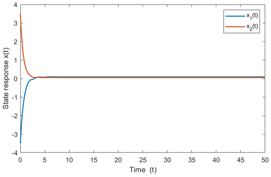
Figure 1 provides the state response of system (4) under zero input and the initial condition $[-3.5,3.5]$. The interval time-varying delays are chosen as $\mu \left(t\right)=[3.6+0.9|sin\left(t\right)\left|\right]$, and the activation function is set as $f\left(\xi \left(t\right)\right)={[0.4tanh\left(x_1\left(t\right)\right),0.8tanh\left(x_2\left(t\right)\right)]}^T$.

Figure 1. It provides the state response of system (4) under zero input and the initial condition $[-3.5,3.5]$. The interval time-varying delays are chosen as $\mu \left(t\right)=[3.6+0.9|sin\left(t\right)\left|\right]$, and the activation function is set as $f\left(\xi \left(t\right)\right)={[0.4tanh\left(x_1\left(t\right)\right),0.8tanh\left(x_2\left(t\right)\right)]}^T$.

The permissible upper bound ${\mu }_M$ for various ${\mu }_d$ is shown in Table 1. Table 1 shows that the conclusions of Remark 3 in this study are less conservative than those in [45,46,47,48], demonstrating the effectiveness of our efforts. Table 1 shows the state variables’ temporal responses. The allowable upper bounds of ${\mu }_M$ are listed in Table 1.

Example 5.

Consider the following matrix parameters for the neural networks matrix parameters:

$$\begin{array}{c}\hfill \dot{\xi }\left(t\right)=-A\xi \left(t\right)+G_{b}f\left(\xi \left(t\right)\right)+G_{d}f\left(\xi (t-\mu \left(t\right))\right),\end{array}$$

with the following:

$$\begin{array}{ccc}\hfill A& =& \left[\begin{array}{cc}1.5& 0\\ 0& 1.7\end{array}\right],G_b=\left[\begin{array}{cc}0.0503& 0.0454\\ 0.0987& 0.2075\end{array}\right],G_d=\left[\begin{array}{cc}0.2381& 0.9320\\ 0.0388& 0.5062\end{array}\right],\hfill \end{array}$$

then $F_1=\mathit{diag}\{0,0\},F_2=\mathit{diag}\{0.3,0.8\}$. The maximum delay bounds with μ calculated by Remark 3, as and the recommended criteria are presented in the Table 2.

Table 2. Allowable upper bound ${\mu }_M$ for various ${\mu }_d$ of Example 5.

Method	${\mathit{\mu }}_{\mathit{d}}=0.4$	${\mathit{\mu }}_{\mathit{d}}=0.45$	${\mathit{\mu }}_{\mathit{d}}=0.5$	${\mathit{\mu }}_{\mathit{d}}=0.55$	Number of Variables
[49]	4.6569	3.7268	3.4076	3.2841	8$n^2$ + 12n
[50]	4.5543	3.8364	3.5583	3.4110	13.5$n^2$ + 21.5n
[51]	7.6697	6.7287	6.4126	3.2569	13.5$n^2$ + 13.5n
[52]	8.3498	7.3817	7.0219	6.8156	7$n^2$ + 11n
Remark 3	9.7901	7.6470	6.7875	6.3190	23$n^2$ + 23n

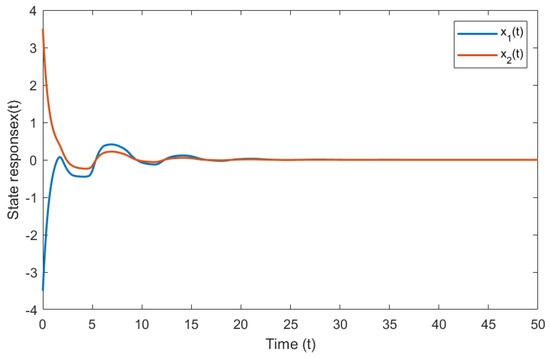
Figure 2 provides the state response of system (4) under zero input and the initial condition $[-3.5,3.5]$. The interval time-varying delays are chosen as $\mu \left(t\right)=[6.3190+0.55|sin\left(t\right)\left|\right]$, and the activation function is set as $f\left(\xi \left(t\right)\right)={[0.3tanh\left(x_1\left(t\right)\right),0.8tanh\left(x_2\left(t\right)\right)]}^T$.

Figure 2. It provides the state response of system (4) under zero input and the initial condition $[-3.5,3.5]$. The interval time-varying delays are chosen as $\mu \left(t\right)=[6.3190+0.55|sin\left(t\right)\left|\right]$, and the activation function is set as $f\left(\xi \left(t\right)\right)={[0.3tanh\left(x_1\left(t\right)\right),0.8tanh\left(x_2\left(t\right)\right)]}^T$.

From Table 2, it follows that Remark 3 provides significantly better results than [49,50,51,52] in the case of ${\mu }_d$ = 0.4 and ${\mu }_d$ = 0.45. However, in cases where ${\mu }_d$ = 0.5 and ${\mu }_d$ = 0.55, the results are slightly worse than in [21]. Additionally, the acquired results are compared to previously published studies. The findings show that the stability conditions presented in this paper are more effective than those found in previous research.

5. Conclusions

In this study, a novel result was presented. The new systems have been used to derive the analysis of finite-time passivity analysis of neutral-type neural networks with mixed time-varying delays. The time-varying delays are distributed, discrete and neutral, and the upper bounds for the delays are available. We are investigating the creation of sufficient conditions for finite boundness, finite-time stability and finite-time passivity, which has not been performed before. First, we create a new Lyapunov–Krasovskii functional, Peng–Park’s integral inequality, descriptor model transformation and zero equation use, and then we used Wirtinger’s integral inequality technique. New finite-time stability necessary conditions are constructed in terms of linear matrix inequalities to guarantee finite-time stability for the system. Finally, numerical examples are presented to demonstrate the result’s effectiveness, and our proposed criteria are less conservative than prior studies in terms of larger time-delay bounds. By combining numerous integral components of the Lyapunov–Krasovskii function with inequality, our results offered wider bounds of time-delay than the previous literature (see Table 1 and Table 2). Construction of an LMI variable number based on integral inequalities yields less conservative stability criteria for interval time-delay systems. We expect to be able to improve existing research and lead research into other areas of application.

References

- Wu, A.; Zeng, Z. Exponential passivity of memristive neural networks with time delays. Neural Netw. 2014, 49, 11–18. [Google Scholar] [CrossRef]
- Gunasekaran, N.; Zhai, G.; Yu, Q. Sampled-data synchronization of delayed multi-agent networks and its application to coupled circuit. Neurocomputing 2020, 413, 499–511. [Google Scholar] [CrossRef]
- Gunasekaran, N.; Thoiyab, N.M.; Muruganantham, P.; Rajchakit, G.; Unyong, B. Novel results on global robust stability analysis for dynamical delayed neural networks under parameter uncertainties. IEEE Access 2020, 8, 178108–178116. [Google Scholar] [CrossRef]
- Wang, H.T.; Liu, Z.T.; He, Y. Exponential stability criterion of the switched neural networks with time-varying delay. Neurocomputing 2019, 331, 1–9. [Google Scholar] [CrossRef]
- Syed Ali, M.; Saravanan, S. Finite-time stability for memristor base d switched neural networks with time-varying delays via average dwell time approach. Neurocomputing 2018, 275, 1637–1649. [Google Scholar]
- Pratap, A.; Raja, R.; Cao, J.; Alzabut, J.; Huang, C. Finite-time synchronization criterion of graph theory perspective fractional-order coupled discontinuous neural networks. Adv. Differ. Equ. 2020, 2020, 97. [Google Scholar] [CrossRef] [Green Version]
- Pratap, A.; Raja, R.; Alzabut, J.; Dianavinnarasi, J.; Cao, J.; Rajchakit, G. Finite-time Mittag-Leffler stability of fractional-order quaternion-valued memristive neural networks with impulses. Neural Process. Lett. 2020, 51, 1485–1526. [Google Scholar] [CrossRef]
- Li, J.; Jiang, H.; Hu, C.; Yu, J. Analysis and discontinuous control for finite-time synchronization of delayed complex dynamical networks. Chaos Solut. Fractals 2018, 114, 219–305. [Google Scholar] [CrossRef]
- Wang, H.; Liu, P.X.; Bao, J.; Xie, X.J.; Li, S. Adaptive neural output-feedback decentralized control for large-scale nonlinear systems with stochastic disturbances. IEEE Trans. Neural Netw. Learn. Syst. 2020, 31, 972–983. [Google Scholar] [CrossRef]
- Zheng, M.; Li, L.; Peng, H.; Xiao, J.; Yang, Y.; Zhang, Y.; Zhao, H. Finite-time stability and synchronization of memristor-based fractional-order fuzzy cellular neural networks. Commun. Nonlinear Sci. Numer. Simul. 2018, 59, 272–297. [Google Scholar] [CrossRef]
- Wu, A.; Zeng, Z. Lagrange stability of memristive neural networks with discrete and distributed delays. IEEE Trans. Neural Netw. Learn. Syst. 2014, 25, 690–703. [Google Scholar] [CrossRef]
- Bai, C.Z. Global stability of almost periodic solutions of Hopfield neural networks with neutral time-varying delays. Appl. Math. Comput. 2008, 203, 72–79. [Google Scholar] [CrossRef]
- Syed Ali, M.; Zhu, Q.; Pavithra, S.; Gunasekaran, N. A study on <(Q,S,R),γ>-dissipative synchronisation of coupled reaction-diffusion neural networks with time-varying delays. Int. J. Syst. Sci. 2017, 49, 755–765. [Google Scholar]
- Chen, Z.; Ruan, J. Global stability analysis of impulsive Cohen-Grossberg neural networks with delay. Phys. Lett. A 2005, 345, 101–111. [Google Scholar] [CrossRef]
- Li, W.J.; Lee, T. Hopfield neural networks for affine invariant matching. IEEE Trans. Neural Netw. Learn. Syst. 2001, 12, 1400–1410. [Google Scholar]
- Syed Ali, M.; Gunasekaran, N.; Zhu, Q. State estimation of T-S fuzzy delayed neural networks with Markovian jumping parameters using sampled-data control. Fuzzy Sets Syst. 2017, 306, 87–104. [Google Scholar] [CrossRef]
- Syed Ali, M.; Narayanana, G.; Sevgenb, S.; Shekher, V.; Arik, S. Global stability analysis of fractional-order fuzzy BAM neural networks with time delay and impulsive effects. Commun. Nonlinear Sci. Numer. Simul. 2019, 78, 104853. [Google Scholar] [CrossRef]
- Samorn, N.; Yotha, N.; Srisilp, P.; Mukdasai, K. LMI-based results on robust exponential passivity of uncertain neutral-type neural networks with mixed interval time-varying delays via the reciprocally convex combination technique. Computation 2021, 9, 70. [Google Scholar] [CrossRef]
- Meesuptong, B.; Mukdasai, K.; Khonchaiyaphum, I. New exponential stability criterion for neutral system with interval time-varying mixed delays and nonlinear uncertainties. Thai J. Math. 2020, 18, 333–349. [Google Scholar]
- Jian, J.; Wang, J. Stability analysis in lagrange sense for a class of BAM neural networks of neutral type with multiple time-varying delays. Neurocomputing 2015, 149, 930–939. [Google Scholar] [CrossRef]
- Lakshmanan, S.; Park, J.H.; Jung, H.Y.; Kwon, O.M.; Rakkiyappan, R. A delay partitioning approach to delay-dependent stability analysis for neutral type neural networks with discrete and distributed delays. Neurocomputing 2013, 111, 81–89. [Google Scholar] [CrossRef]
- Peng, W.; Wu, Q.; Zhang, Z. LMI-based global exponential stability of equilibrium point for neutral delayed BAM neural networks with delays in leakage terms via new inequality technique. Neurocomputing 2016, 199, 103–113. [Google Scholar] [CrossRef]
- Syed Ali, M.; Saravanakumar, R.; Cao, J. New passivity criteria for memristor-based neutral-type stochastic BAM neural networks with mixed time-varying delays. Neurocomputing 2016, 171, 1533–1547. [Google Scholar] [CrossRef]
- Klamnoi, A.; Yotha, N.; Weera, W.; Botmart, T. Improved results on passivity analysis of neutral-type neural networks with mixed time-varying delays. J. Res. Appl. Mech. Eng. 2018, 6, 71–81. [Google Scholar]
- Ding, D.; Wang, Z.; Dong, H.; Shu, H. Distributed H∞ state estimation with stochastic parameters and nonlinearities through sensor networks: The finite-horizon case. Automatica 2012, 48, 1575–1585. [Google Scholar] [CrossRef]
- Carrasco, J.; Baños, A.; Schaft, A.V. A passivity-based approach to reset control systems stability January. Syst. Control Lett. 2010, 59, 18–24. [Google Scholar] [CrossRef] [Green Version]
- Krasovskii, N.N.; Lidskii, E.A. Analytical design of controllers in systems with random attributes. Autom. Remote Control 1961, 22, 1021–1025. [Google Scholar]
- Debeljković, D.; Stojanović, S.; Jovanović, A. Finite-time stability of continuous time delay systems: Lyapunov-like approach with Jensen’s and Coppel’s inequality. Acta Polytech. Hung. 2013, 10, 135–150. [Google Scholar]
- Wang, L.; Shen, Y.; Ding, Z. Finite time stabilization of delayed neural networks. Neural Netw. 2015, 70, 74–80. [Google Scholar] [CrossRef] [PubMed]
- Rajavela, S.; Samiduraia, R.; Caobc, J.; Alsaedid, A.; Ahmadd, B. Finite-time non-fragile passivity control for neural networks with time-varying delay. Appl. Math. Comput. 2017, 297, 145–158. [Google Scholar] [CrossRef]
- Chen, X.; He, S. Finite-time passive filtering for a class of neutral time-delayed systems. Trans. Inst. Meas. Control 2016, 1139–1145. [Google Scholar] [CrossRef]
- Syed Ali, M.; Saravanan, S.; Zhu, Q. Finite-time stability of neutral-type neural networks with random time-varying delays. Syst. Sci. 2017, 48, 3279–3295. [Google Scholar]
- Saravanan, S.; Syed Ali, M.; Alsaedib, A.; Ahmadb, B. Finite-time passivity for neutral-type neural networks with time-varying delays. Nonlinear Anal. Model. Control 2020, 25, 206–224. [Google Scholar]
- Syed Ali, M.; Meenakshi, K.; Gunasekaran, N. Finite-time H∞ boundedness of discrete-time neural networks normbounded disturbances with time-varying delay. Int. J. Control Autom. Syst. 2017, 15, 2681–2689. [Google Scholar] [CrossRef]
- Phanlert, C.; Botmart, T.; Weera, W.; Junsawang, P. Finite-Time Mixed H∞/passivity for neural networks with mixed interval time-varying delays using the multiple integral Lyapunov-Krasovskii functional. IEEE Access 2021, 9, 89461–89475. [Google Scholar] [CrossRef]
- Amato, F.; Ariola, M.; Dorato, P. Finite-time control of linear systems subject to parametric uncertainties and disturbances. Automatica 2001, 37, 1459–1463. [Google Scholar] [CrossRef]
- Song, J.; He, S. Finite-time robust passive control for a class of uncertain Lipschitz nonlinear systems with time-delays. Neurocomputing 2015, 159, 275–281. [Google Scholar] [CrossRef]
- Kwon, O.M.; Park, M.J.; Park, J.H.; Lee, S.M.; Cha, E.J. New delay-partitioning approaches to stability criteria for uncertain neutral systems with time-varying delays. SciVerse Sci. Direct 2012, 349, 2799–2823. [Google Scholar] [CrossRef]
- Seuret, A.; Gouaisbaut, F. Wirtinger-based integral inequality: Application to time-delay system. Automatica 2013, 49, 2860–2866. [Google Scholar] [CrossRef] [Green Version]
- Peng, C.; Fei, M.R. An improved result on the stability of uncertain T-S fuzzy systems with interval time-varying delay. Fuzzy Sets Syst. 2013, 212, 97–109. [Google Scholar] [CrossRef]
- Park, P.G.; Ko, J.W.; Jeong, C.K. Reciprocally convex approach to stability of systems with time-varying delays. Automatica 2011, 47, 235–238. [Google Scholar] [CrossRef]
- Kwon, O.M.; Park, M.J.; Park, J.H.; Lee, S.M.; Cha, E.J. Analysis on robust H∞ performance and stability for linear systems with interval time-varying state delays via some new augmented Lyapunov Krasovskii functional. Appl. Math. Comput. 2013, 224, 108–122. [Google Scholar]
- Singkibud, P.; Niamsup, P.; Mukdasai, K. Improved results on delay-rage-dependent robust stability criteria of uncertain neutral systems with mixed interval time-varying delays. IAENG Int. J. Appl. Math. 2017, 47, 209–222. [Google Scholar]
- Tian, J.; Ren, Z.; Zhong, S. A new integral inequality and application to stability of time-delay systems. Appl. Math. Lett. 2020, 101, 106058. [Google Scholar] [CrossRef]
- Kwon, O.M.; Park, J.H.; Lee, S.M.; Cha, E.J. New augmented Lyapunov-Krasovskii functional approach to stability analysis of neural networks with time-varying delays. Nonlinear Dyn. 2014, 76, 221–236. [Google Scholar] [CrossRef]
- Zeng, H.B.; He, Y.; Wu, M.; Xiao, S.P. Stability analysis of generalized neural networks with time-varying delays via a new integral inequality. Neurocomputing 2015, 161, 148–154. [Google Scholar] [CrossRef]
- Yang, B.; Wang, J. Stability analysis of delayed neural networks via a new integral inequality. Neural Netw. 2017, 88, 49–57. [Google Scholar] [CrossRef]
- Hua, C.; Wang, Y.; Wu, S. Stability analysis of neural networks with time-varying delay using a new augmented Lyapunov-Krasovskii functional. Neurocomputing 2019, 332, 1–9. [Google Scholar] [CrossRef]
- Zhu, X.L.; Yue, D.; Wang, Y. Delay-dependent stability analysis for neural networks with additive time-varying delay components. IET Control Theory Appl. 2013, 7, 354–362. [Google Scholar] [CrossRef]
- Li, T.; Wang, T.; Song, A.; Fei, S. Combined convex technique on delay-dependent stability for delayed neural networks. IEEE Trans. Neural Netw. Learn. Syst. 2013, 24, 1459–1466. [Google Scholar] [CrossRef]
- Zhang, C.K.; He, Y.; Jiang, L.; Wu, M. Stability analysis for delayed neural networks considering both conservativeness and complexity. IEEE Trans. Neural Netw. Learn. Syst. 2015, 27, 1486–1501. [Google Scholar] [CrossRef] [PubMed] [Green Version]
- Zhang, C.K.; He, Y.; Jiang, L.; Lin, W.J.; Wu, M. Delay-dependent stability analysis of neural networks with time-varying delay: A generalized free-weighting-matrix approach. Appl. Math. Comput. 2017, 294, 102–120. [Google Scholar] [CrossRef]
Publisher’s Note: MDPI stays neutral with regard to jurisdictional claims in published maps and institutional affiliations. |
© 2021 by the authors. Licensee MDPI, Basel, Switzerland. This article is an open access article distributed under the terms and conditions of the Creative Commons Attribution (CC BY) license (https://creativecommons.org/licenses/by/4.0/).