Hierarchical Quasi-Fractional Gradient Descent Method for Parameter Estimation of Nonlinear ARX Systems Using Key Term Separation Principle

Abstract

Recently, a quasi-fractional order gradient descent (QFGD) algorithm was proposed and successfully applied to solve system identification problem. The QFGD suffers from the overparameterization problem and results in estimating the redundant parameters instead of identifying only the actual parameters of the system. This study develops a novel hierarchical QFDS (HQFGD) algorithm by introducing the concepts of hierarchical identification principle and key term separation idea. The proposed HQFGD is effectively applied to solve the parameter estimation problem of input nonlinear autoregressive with exogeneous noise (INARX) system. A detailed investigation about the performance of HQFGD is conducted under different disturbance conditions considering different fractional orders and learning rate variations. The simulation results validate the better performance of the HQFGD over the standard counterpart in terms of estimation accuracy, convergence speed and robustness.

1. Introduction

Fractional calculus has emerged as an important tool to effectively model a variety of systems or processes that arise in the various applications relating to physics, engineering and applied sciences [1,2,3,4,5,6,7,8]. Over the last decade, a trend of developing novel adaptive algorithms based on strong foundations of fractional calculus can be seen [9,10,11,12,13,14,15]. The idea of incorporating the fractional derivative into the conventional iterative procedure of the least mean square (LMS) algorithm was first introduced in 2009 [16]. The fractional derivative-based LMS, i.e., F-LMS, was then exploited to solve communication [17,18,19], vibration rejection [20], control [21], recommender systems [22,23], power signal modelling [24], signal processing [25] and time series prediction problems [26]. The variants of the F-LMS were proposed to solve different identification and parameter estimation problems [27,28,29,30,31]. Cheng et al. presented the concept of a variable initial value and proposed an innovative F-LMS (IF-LMS) [32], and Chaudhary et al. applied the IF-LMS for the parameter estimation of power signals [33]. Chen et al. compared the performance of different fractional order gradient methods [34]. Wei. et al. suggested a modification to handle a long memory property of fractional calculus and proposed a generalized fractional order gradient method (GFGM) [35]. Liu et al. generalized the GFGM to solve convex optimization problem with high dimensions, and proposed a quasi-fractional gradient (QFGD) method with theoretical analysis and convergence proof [36]. Furthermore, they also applied QFGD to solve system identification problem through overparameterization and estimated the redundant parameters instead of estimating only the actual parameters of the system. In order to avoid the problem of overparameterization, we propose hierarchical QFGD (HQFGD) by integrating the hierarchical identification principle and key term separation idea with QFGD for efficient parameter estimation. The hierarchical identification principle decomposes the system into multiple subsystems, thus reducing the overall dimensions of the system, and the key term separation technique allows one to avoid the overparameterization issue [37,38,39]. In this study, we propose HQFGD method for efficient parameter estimation of input nonlinear autoregressive exogenous noise (INARX) systems. The INARX system belongs to a class of block-oriented nonlinear systems that are widely used to model a variety of nonlinearities [40,41,42,43]. The main contributions of this study in terms of salient features are summarized as:

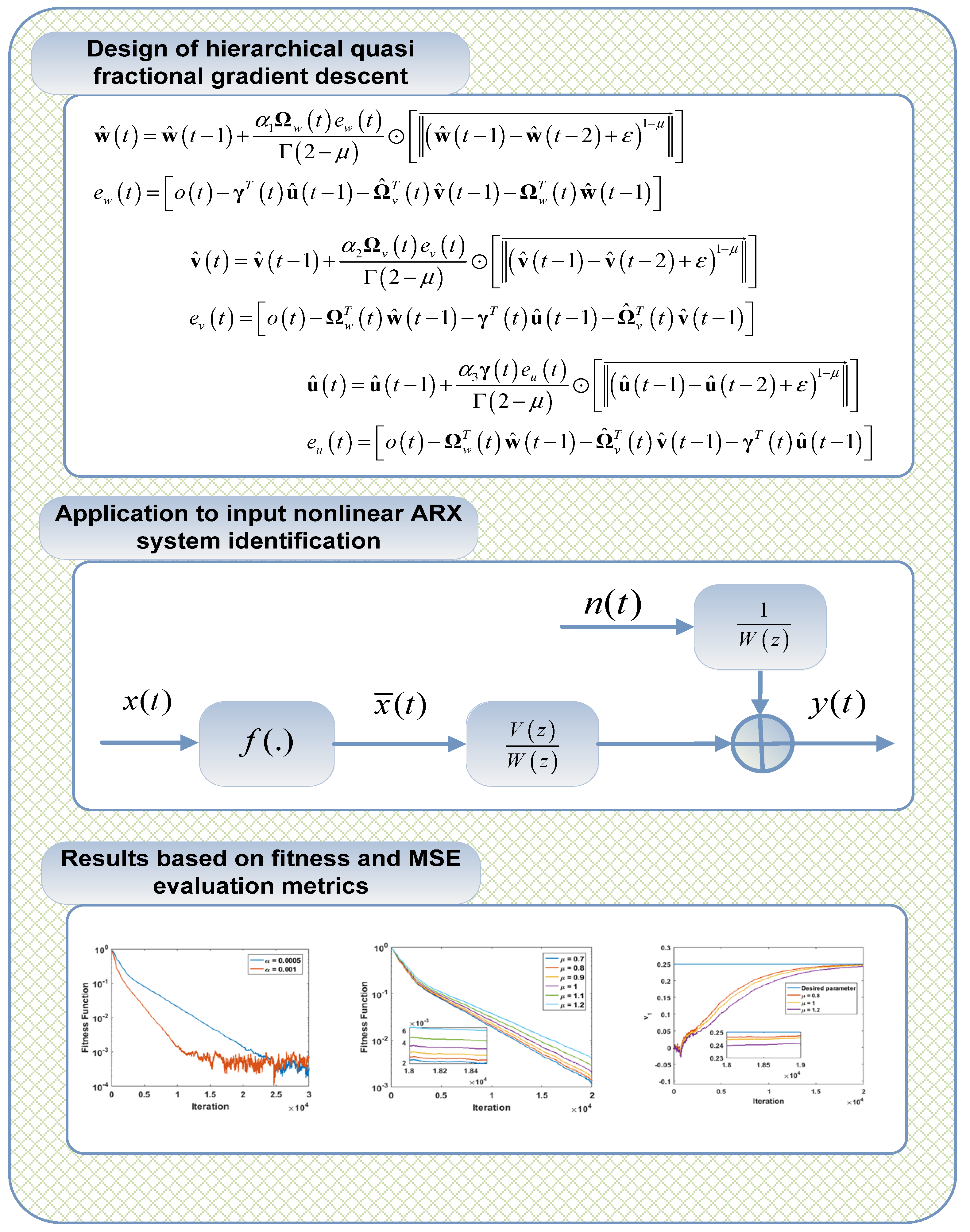
• A novel hierarchical quasi-fractional gradient descent, HQFGD, algorithm is presented by integrating the hierarchical identification theory and key term separation technique with the quasi-fractional gradient method.
• The hierarchical identification procedure decomposes the system into subsystems, thus reducing the overall dimensions of the system, and the key term separation technique allows one to avoid the overparameterization issue.
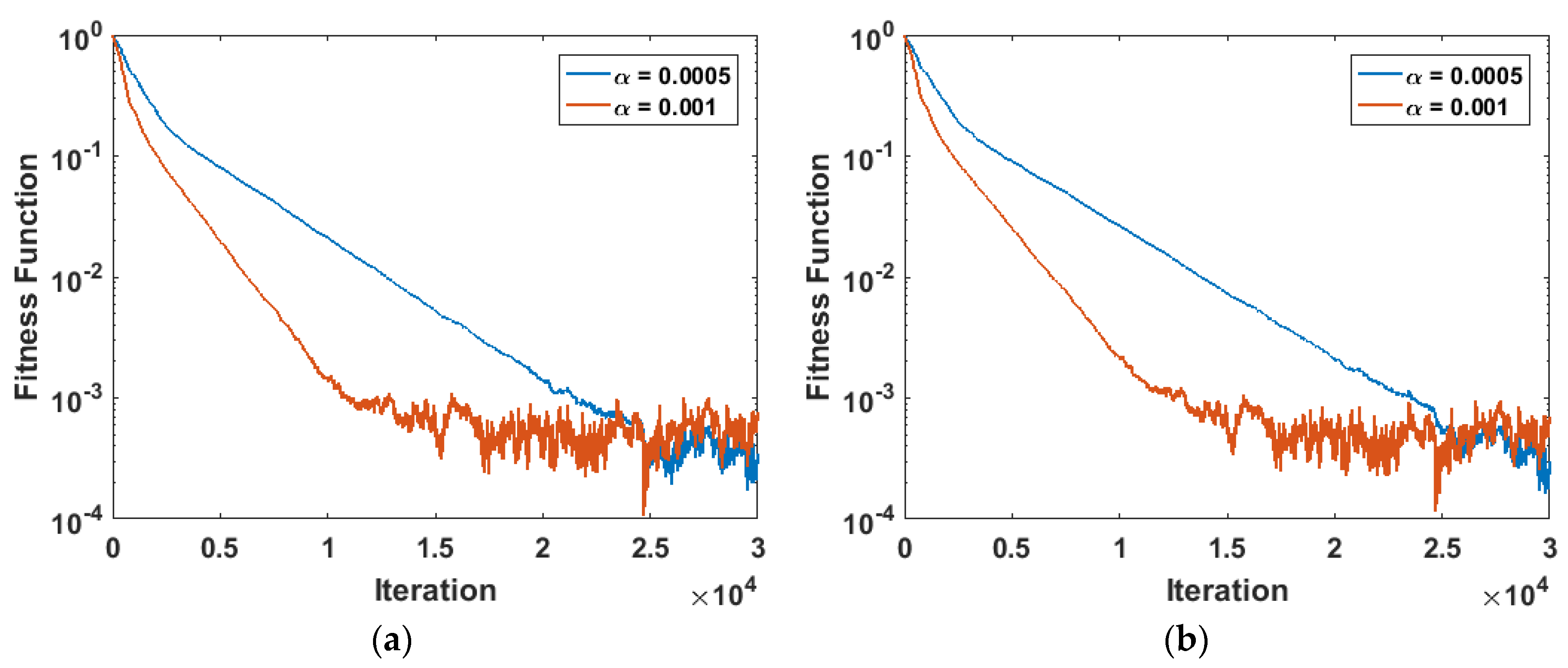
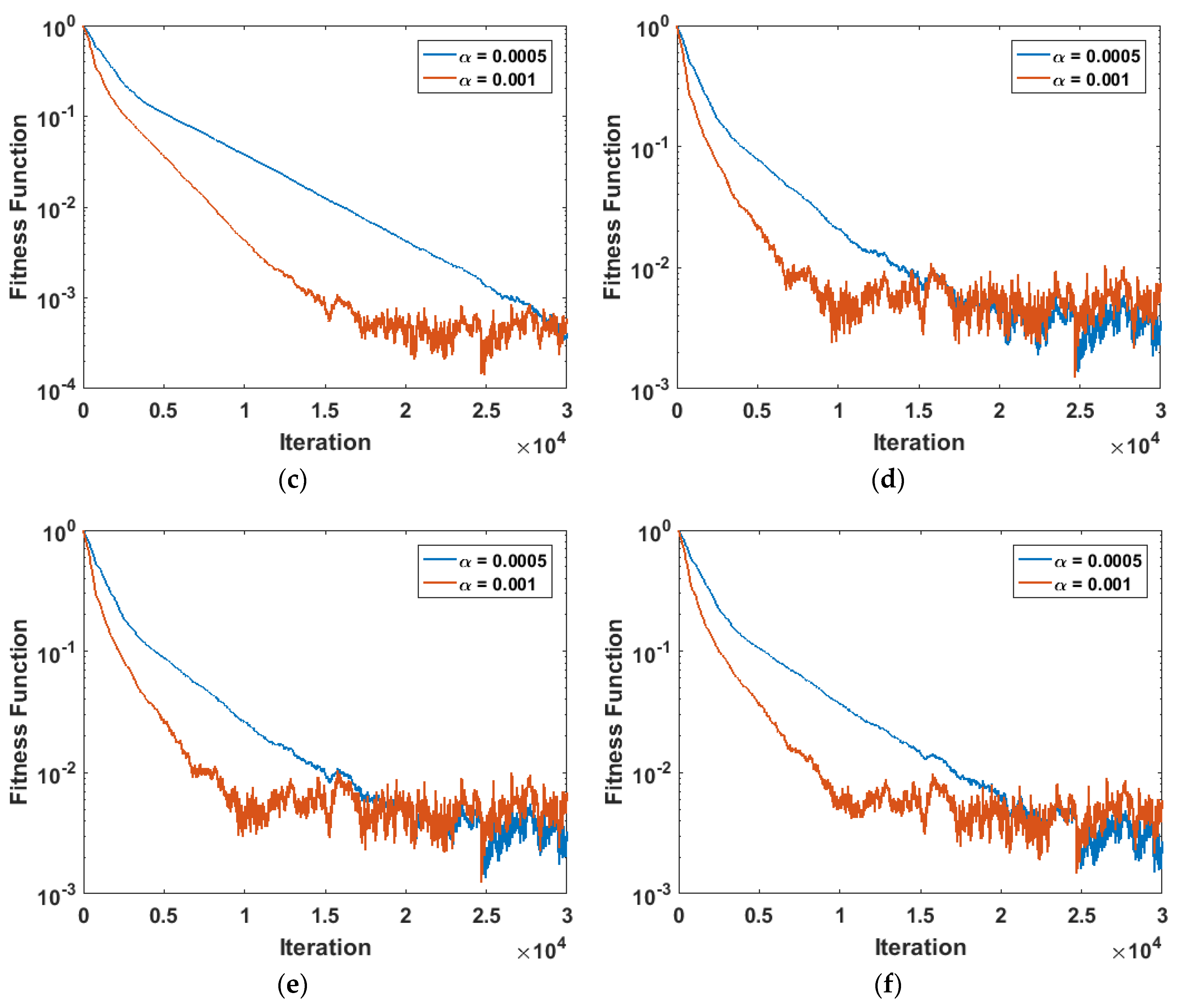
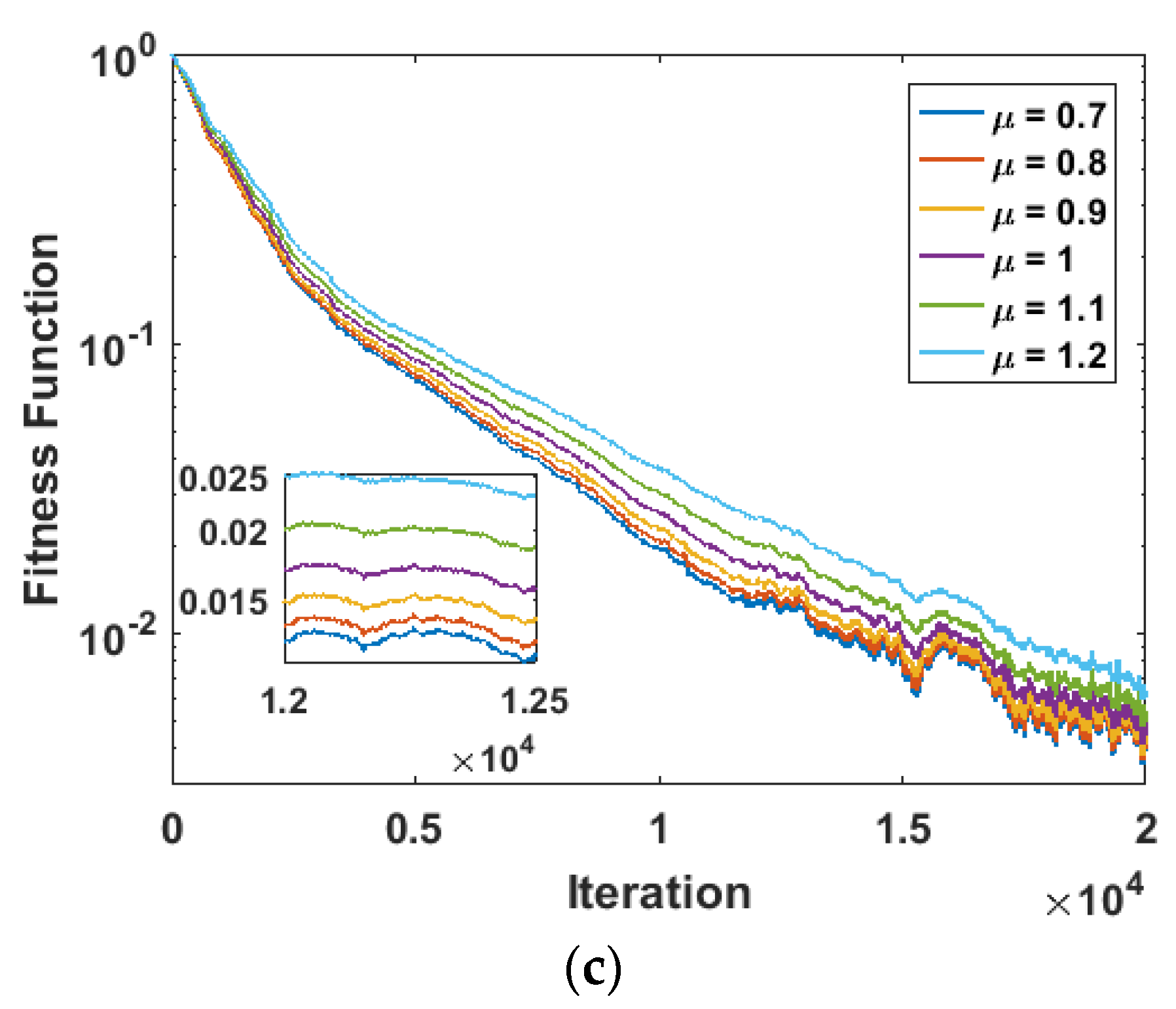
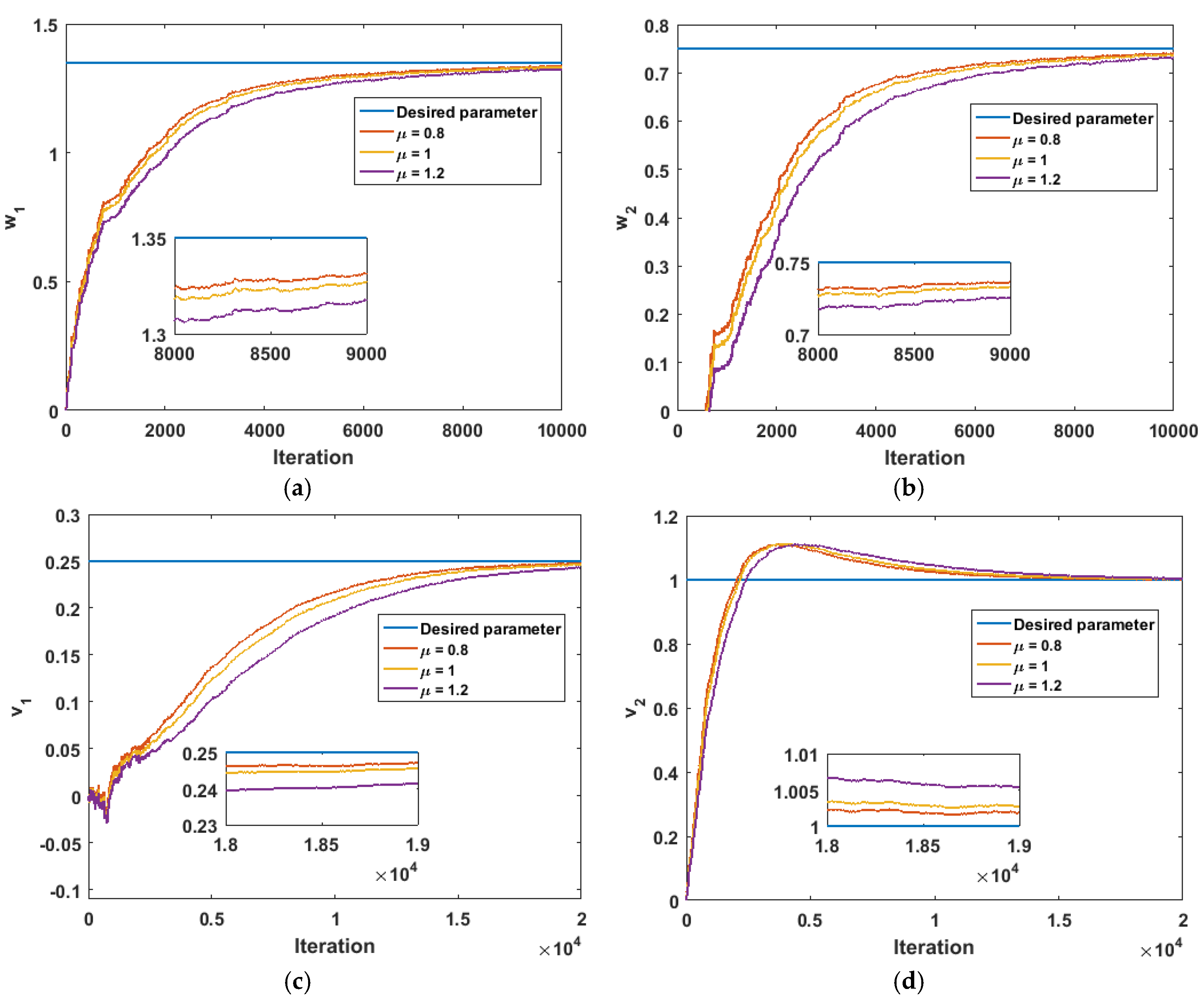
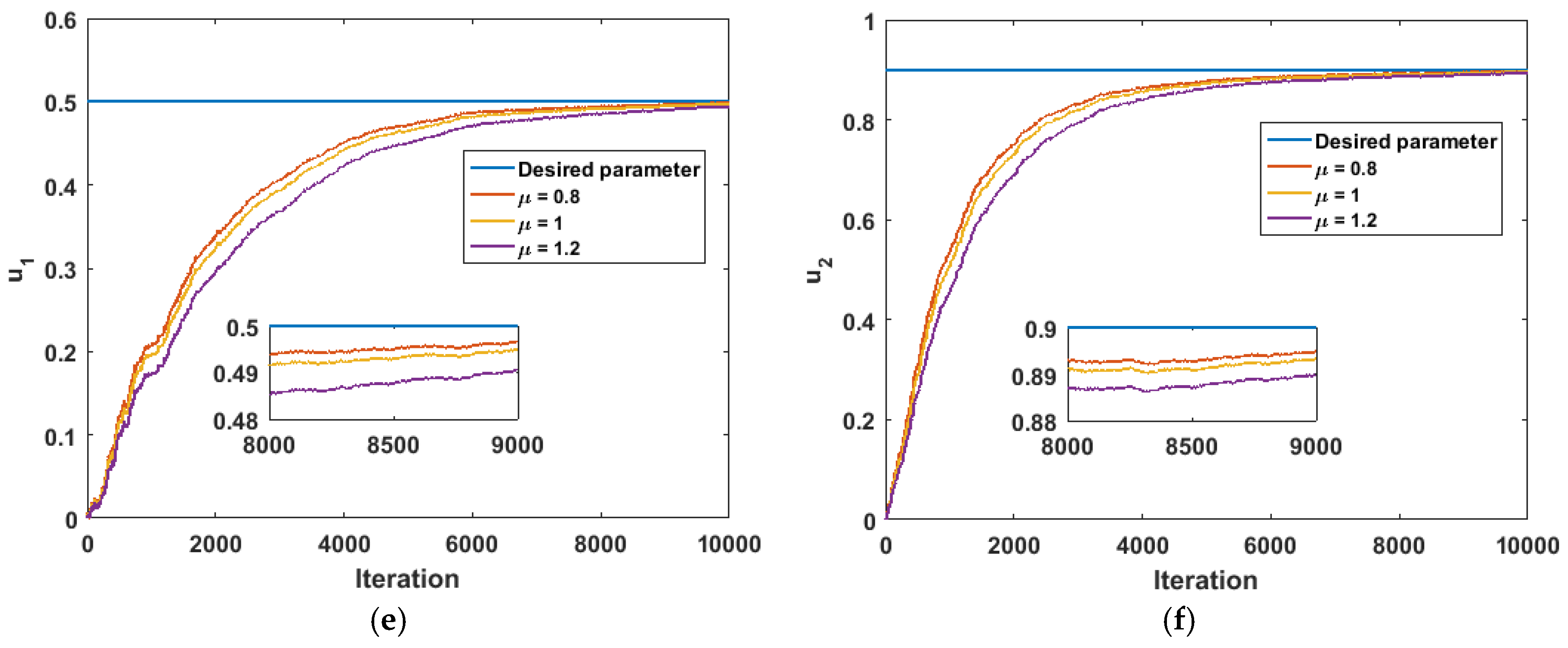
• The accuracy and robustness of the proposed HQFGD is established through effective parameter estimation of input nonlinear autoregressive exogenous noise, INARX, systems under different disturbance conditions, fractional orders and learning rate variations.
• The comparison with the standard counterpart validates the efficacy of the proposed HQFGD scheme in terms of convergence sped and estimation accuracy.

The remainder of this paper is structured as follows: Section 2 gives the description of the INARX system. Section 3 describes the HGD approach and Section 4 provides the design of the hierarchical QFGD for INARX systems. Section 5 discusses the results of numerical experimentation and Section 6 presents the conclusions with some future works.

2. Nonlinear ARX System Model

The governing mathematical relation of the INARX system with input x, output y, and exogeneous noise n is written as [44,45]:

$$o(t)=\frac{V(z)}{W(z)}\overline{x}(t)+\frac{1}{W(z)}n(t),$$

(1)

where $W(z)$, $V(z)$ and $\overline{x}\left(t\right)$ are defined as

$$W\left(z\right)=1+w_1{z}^{-1}+w_2{z}^{-2}+,\dots ,+w_{n_w}{z}^{-n_w},$$

(2)

$$V\left(z\right)=r_0+v_1{z}^{-1}+v_2{z}^{-2}+,\dots ,+v_{n_v}{z}^{-n_v},$$

(3)

$$\overline{x}\left(t\right)=u_1{\gamma }_1\left(x\left(t\right)\right)+u_2{\gamma }_2\left(x\left(t\right)\right)+\dots +u_p{\gamma }_p\left(x\left(t\right)\right).$$

(4)

Rewriting (1) after rearranging,

$$o(t)=\left(1-W(z)\right)o\left(t\right)+V(z)\overline{x}(t)+n(t).$$

(5)

Putting Expressions (2)–(4) into (5), let $v_0=1$, and considering $\overline{x}\left(t\right)$ as a key term, apply key term separation:

$$\begin{array}{ll}o(t)& =-{\displaystyle \sum _{k=1}^{n_w}{w}_k}o\left(t-k\right)+{\displaystyle \sum _{k=0}^{n_v}{v}_k}\overline{x}\left(t-k\right)+n(t)\\ & =-{\displaystyle \sum _{k=1}^{n_w}{w}_k}o\left(t-k\right)+v_0\overline{x}\left(t\right)+{\displaystyle \sum _{k=1}^{n_v}{v}_k}\overline{x}\left(t-k\right)+n(t)\\ & =-{\displaystyle \sum _{k=1}^{n_w}{w}_k}o\left(t-k\right)+{\displaystyle \sum _{k=1}^{n_v}{v}_k}\overline{x}\left(t-k\right)+{\displaystyle \sum _{i=1}^p{u}_i{\gamma }_i\left(x\left(t\right)\right)}+n(t)\end{array}$$

(6)

The information vector is defined as:

$$\begin{array}{l}{\Omega }_w\left(t\right)={\left[-o\left(t-1\right),-o\left(t-2\right),\dots ,-o\left(t-n_w\right)\right]}^T\in {ℝ}^{n_w}\\ {\Omega }_v\left(t\right)={\left[\overline{x}\left(t-1\right),\overline{x}\left(t-2\right),\dots ,\overline{x}\left(t-n_v\right)\right]}^T\in {ℝ}^{n_v}\\ \gamma \left(t\right)={\left[{\gamma }_1\left(u\left(t\right)\right),{\gamma }_2\left(u\left(t\right)\right),\dots ,{\gamma }_p\left(u\left(t\right)\right)\right]}^T\in {ℝ}^p\end{array}$$

(7)

and the corresponding parameter vectors are:

$$\begin{array}{l}w={\left[w_1,w_2,\dots ,w_{n_w}\right]}^T\in {ℝ}^{n_w}\\ v={\left[v_1,v_2,\dots ,v_{n_v}\right]}^T\in {ℝ}^{n_v}\\ u={\left[u_1,u_2,\dots ,u_p\right]}^T\in {ℝ}^p\end{array}$$

(8)

Putting (7) and (8) into (6), the output of the INARX system using key term separation [37] is written as:

$$o\left(t\right)={\Omega }_w^T\left(t\right)w+{\Omega }_v^T\left(t\right)v+{\gamma }^T\left(t\right)u+n\left(t\right).$$

(9)

3. Hierarchical Gradient Descent Method

The brief overview of hierarchical identification based gradient descent (HGD) is presented in this section. The intermediate variables are defined as:

$$o_w\left(t\right)=o\left(t\right)-{\Omega }_v^T\left(t\right)v-{\gamma }^T\left(t\right)u,$$

(10)

$$o_v\left(t\right)=o\left(t\right)-{\Omega }_w^T\left(t\right)w-{\gamma }^T\left(t\right)u,$$

(11)

$$o_u\left(t\right)=o\left(t\right)-{\Omega }_w^T\left(t\right)w-{\Omega }_v^T\left(t\right)v,$$

(12)

Decomposing (9) into three sub-systems:

$$o_w\left(t\right)={\Omega }_w^T\left(t\right)w+n(t),$$

(13)

$$o_v\left(t\right)={\Omega }_v^T\left(t\right)v+n(t),$$

(14)

$$o_u\left(t\right)={\gamma }^T\left(t\right)u+n(t).$$

(15)

From (13)–(15), the cost functions are defined as:

$$J_w\left(w\right)={\left(o_w\left(t\right)-{\Omega }_w^T\left(t\right)w\right)}^2,$$

(16)

$$J_v\left(v\right)={\left(o_v\left(t\right)-{\Omega }_v^T\left(t\right)v\right)}^2,$$

(17)

$$J_u\left(u\right)={\left(o_u\left(t\right)-{\gamma }^T\left(t\right)u\right)}^2.$$

(18)

The following update rules are obtained by minimizing cost functions (16)–(18) through the gradient descent approach:

$$\begin{array}{ll}\widehat{w}\left(t\right)& =\widehat{w}\left(t-1\right)+{\alpha }_1{\Omega }_w\left(t\right)\left[o_w\left(t\right)-{\Omega }_w^T\left(t\right)\widehat{w}\left(t-1\right)\right]\\ & =\widehat{w}\left(t-1\right)+{\alpha }_1{\Omega }_w\left(t\right)\left[o\left(t\right)-{\Omega }_v^T\left(t\right)v\left(t-1\right)-{\gamma }^T\left(t\right)\widehat{u}\left(t-1\right)-{\Omega }_w^T\left(t\right)\widehat{w}\left(t-1\right)\right]\end{array}$$

(19)

$$\begin{array}{ll}\widehat{v}\left(t\right)& =\widehat{v}\left(t-1\right)+{\alpha }_2{\Omega }_v\left(t\right)\left[o_r\left(t\right)-{\Omega }_v^T\left(t\right)\widehat{v}\left(t-1\right)\right]\\ & =\widehat{v}\left(t-1\right)+{\alpha }_2{\Omega }_v\left(t\right)\left[o\left(t\right)-{\Omega }_w^T\left(t\right)\widehat{w}\left(t-1\right)-{\gamma }^T\left(t\right)\widehat{u}\left(t-1\right)-{\Omega }_v^T\left(t\right)\widehat{v}\left(t-1\right)\right]\end{array}$$

(20)

$$\begin{array}{ll}\widehat{u}\left(t\right)& =\widehat{u}\left(t-1\right)+{\alpha }_3\gamma \left(t\right)\left[o_u\left(t\right)-{\gamma }^T\left(t\right)\widehat{u}\left(t-1\right)\right]\\ & =\widehat{u}\left(t-1\right)+{\alpha }_3\gamma \left(t\right)\left[o\left(t\right)-{\Omega }_w^T\left(t\right)\widehat{w}\left(t-1\right)-{\Omega }_v^T\left(t\right)\widehat{v}\left(t-1\right)-{\gamma }^T\left(t\right)\widehat{u}\left(t-1\right)\right]\end{array}$$

(21)

There are unmeasurable inner terms in ${\Omega }_v\left(t\right)$ of (19)–(21), whose estimation is defined as:

$${\widehat{\Omega }}_v\left(t\right)={\left[\widehat{\overline{x}}\left(t-1\right),\hspace{0.17em}\widehat{\overline{x}}\left(t-2\right),\hspace{0.17em}\dots \hspace{0.17em},\hspace{0.17em}\widehat{\overline{x}}\left(t-n_v\right)\right]}^T,$$

(22)

$$\widehat{\overline{x}}\left(t\right)={\displaystyle \sum _{i=1}^p{\widehat{u}}_i\left(t\right){\gamma }_i\left(x\left(t\right)\right)}={\gamma }^T\left(t\right)\widehat{u}\left(t\right).$$

(23)

Replacing ${\Omega }_v\left(t\right)$ with ${\widehat{\Omega }}_v\left(t\right)$ in (19)–(21) gives the HGD for INARX identification:

$$\widehat{w}\left(t\right)=\widehat{w}\left(t-1\right)+{\alpha }_1{\Omega }_w\left(t\right)\left[o\left(t\right)-{\widehat{\Omega }}_v^T\left(t\right)v\left(t-1\right)-{\gamma }^T\left(t\right)\widehat{u}\left(t-1\right)-{\Omega }_w^T\left(t\right)\widehat{w}\left(t-1\right)\right],$$

(24)

$$\widehat{v}\left(t\right)=\widehat{v}\left(t-1\right)+{\alpha }_2{\Omega }_v\left(t\right)\left[o\left(t\right)-{\Omega }_w^T\left(t\right)\widehat{w}\left(t-1\right)-{\gamma }^T\left(t\right)\widehat{u}\left(t-1\right)-{\widehat{\Omega }}_v^T\left(t\right)\widehat{v}\left(t-1\right)\right],$$

(25)

$$\widehat{u}\left(t\right)=\widehat{u}\left(t-1\right)+{\alpha }_3\gamma \left(t\right)\left[o\left(t\right)-{\Omega }_w^T\left(t\right)\widehat{w}\left(t-1\right)-{\widehat{\Omega }}_v^T\left(t\right)\widehat{v}\left(t-1\right)-{\gamma }^T\left(t\right)\widehat{u}\left(t-1\right)\right].$$

(26)

4. Hierarchical Quasi Fractional Gradient Descent Method

In this section, the design of the proposed hierarchical quasi fractional gradient descent HQFGD is presented. The general iterative update rule of QFGD for a multi-variable function $f\left(s\right)$ is written as reported in the recent literature [36]:

$$s\left(t\right)=s\left(t-1\right)-\frac{\alpha }{\Gamma \left(2-\mu \right)}\nabla {f\left(s\right)|}_{t=t-1}\odot \left[\overrightarrow{\Vert {\left(s\left(t-1\right)-s\left(t-2\right)+\epsilon \right)}^{1-\mu }\Vert }\right],$$

(27)

where $0<\mu <2$ is the fractional order, $\alpha$ is the learning rate, $\epsilon$ is a vector of small numbers, $\nabla$ is the conventional first order gradient, $\Vert ·\Vert$ denotes the 2 norms of a vector, and $\odot$ represents the Hadamard product. The search direction in QFGD is produced through the Hadamard product between the direction of the fractional gradient and another vector on the basis of the fractional gradient direction, as described in [36]. This helps in avoiding zigzag during gradient descent search by rotating the fractional gradient direction. Thus, $\nabla {f\left(s\right)|}_{t=t-1}\odot \left[\overrightarrow{\Vert {\left(s\left(t-1\right)-s\left(t-2\right)+\epsilon \right)}^{1-\mu }\Vert }\right]$ is called the QFGD direction. Further details about QFGD can be seen in [36].

Minimizing the cost functions (16)–(18) by using (27), the iterative update relations of the QFGD for $w,\hspace{0.17em}v,\hspace{0.17em}u$ are written as:

$$\widehat{w}\left(t\right)=\widehat{w}\left(t-1\right)+\frac{{\alpha }_1{\Omega }_w\left(t\right)}{\Gamma \left(2-\mu \right)}\left[o_w\left(t\right)-{\Omega }_w^T\left(t\right)\widehat{w}\left(t-1\right)\right]\odot \left[\overrightarrow{\Vert {\left(\widehat{w}\left(t-1\right)-\widehat{w}\left(t-2\right)+\epsilon \right)}^{1-\mu }\Vert }\right],$$

(28)

$$\widehat{v}\left(t\right)=\widehat{v}\left(t-1\right)+\frac{{\alpha }_2{\Omega }_v\left(t\right)}{\Gamma \left(2-\mu \right)}\left[o_v\left(t\right)-{\Omega }_v^T\left(t\right)\widehat{v}\left(t-1\right)\right]\odot \left[\overrightarrow{\Vert {\left(\widehat{v}\left(t-1\right)-\widehat{v}\left(t-2\right)+\epsilon \right)}^{1-\mu }\Vert }\right],$$

(29)

$$\widehat{u}\left(t\right)=\widehat{u}\left(t-1\right)+\frac{{\alpha }_3\gamma \left(t\right)}{\Gamma \left(2-\mu \right)}\left[o_u\left(t\right)-\gamma \left(t\right)\widehat{u}\left(t-1\right)\right]\odot \left[\overrightarrow{\Vert {\left(\widehat{u}\left(t-1\right)-\widehat{u}\left(t-2\right)+\epsilon \right)}^{1-\mu }\Vert }\right].$$

(30)

Using (10)–(12) in (28)–(30), respectively:

$$\widehat{w}\left(t\right)=\widehat{w}\left(t-1\right)+\frac{{\alpha }_1{\Omega }_w\left(t\right)e_w\left(t\right)}{\Gamma \left(2-\mu \right)}\odot \left[\overrightarrow{\Vert {\left(\widehat{w}\left(t-1\right)-\widehat{w}\left(t-2\right)+\epsilon \right)}^{1-\mu }\Vert }\right],$$

(31)

$$\widehat{v}\left(t\right)=\widehat{v}\left(t-1\right)+\frac{{\alpha }_2{\Omega }_v\left(t\right)e_v\left(t\right)}{\Gamma \left(2-\mu \right)}\odot \left[\overrightarrow{\Vert {\left(\widehat{v}\left(t-1\right)-\widehat{v}\left(t-2\right)+\epsilon \right)}^{1-\mu }\Vert }\right],$$

(32)

$$\widehat{u}\left(t\right)=\widehat{u}\left(t-1\right)+\frac{{\alpha }_3\gamma \left(t\right)e_u\left(t\right)}{\Gamma \left(2-\mu \right)}\odot \left[\overrightarrow{\Vert {\left(\widehat{u}\left(t-1\right)-\widehat{u}\left(t-2\right)+\epsilon \right)}^{1-\mu }\Vert }\right],$$

(33)

where $e_w$, $e_v$ and $e_u$ are defined as:

$$e_w\left(t\right)=\left[o\left(t\right)-{\gamma }^T\left(t\right)\widehat{u}\left(t-1\right)-{\Omega }_v^T\left(t\right)\widehat{v}\left(t-1\right)-{\Omega }_w^T\left(t\right)\widehat{w}\left(t-1\right)\right],$$

$$e_v\left(t\right)=\left[o\left(t\right)-{\Omega }_w^T\left(t\right)\widehat{w}\left(t-1\right)-{\gamma }^T\left(t\right)\widehat{u}\left(t-1\right)-{\Omega }_v^T\left(t\right)\widehat{v}\left(t-1\right)\right],$$

$$e_u\left(t\right)=\left[o\left(t\right)-{\Omega }_w^T\left(t\right)\widehat{w}\left(t-1\right)-{\Omega }_v^T\left(t\right)\widehat{v}\left(t-1\right)-{\gamma }^T\left(t\right)\widehat{u}\left(t-1\right)\right].$$

Using (22)–(23) to replace ${\Omega }_v\left(t\right)$ with estimate ${\widehat{\Omega }}_v\left(t\right)$ in (31)–(33) gives the hierarchical QFGD method for parameter estimation of INARX systems:

$$\begin{array}{l}\widehat{w}\left(t\right)=\widehat{w}\left(t-1\right)+\frac{{\alpha }_1{\Omega }_w\left(t\right)e_w\left(t\right)}{\Gamma \left(2-\mu \right)}\odot \left[\overrightarrow{\Vert {\left(\widehat{w}\left(t-1\right)-\widehat{w}\left(t-2\right)+\epsilon \right)}^{1-\mu }\Vert }\right]\\ e_w\left(t\right)=\left[o\left(t\right)-{\gamma }^T\left(t\right)\widehat{u}\left(t-1\right)-{\widehat{\Omega }}_v^T\left(t\right)\widehat{v}\left(t-1\right)-{\Omega }_w^T\left(t\right)\widehat{w}\left(t-1\right)\right]\end{array}$$

(34)

$$\begin{array}{l}\widehat{v}\left(t\right)=\widehat{v}\left(t-1\right)+\frac{{\alpha }_2{\Omega }_v\left(t\right)e_v\left(t\right)}{\Gamma \left(2-\mu \right)}\odot \left[\overrightarrow{\Vert {\left(\widehat{v}\left(t-1\right)-\widehat{v}\left(t-2\right)+\epsilon \right)}^{1-\mu }\Vert }\right]\\ e_v\left(t\right)=\left[o\left(t\right)-{\Omega }_w^T\left(t\right)\widehat{w}\left(t-1\right)-{\gamma }^T\left(t\right)\widehat{u}\left(t-1\right)-{\widehat{\Omega }}_v^T\left(t\right)\widehat{v}\left(t-1\right)\right]\end{array}$$

(35)

$$\begin{array}{l}\widehat{u}\left(t\right)=\widehat{u}\left(t-1\right)+\frac{{\alpha }_3\gamma \left(t\right)e_u\left(t\right)}{\Gamma \left(2-\mu \right)}\odot \left[\overrightarrow{\Vert {\left(\widehat{u}\left(t-1\right)-\widehat{u}\left(t-2\right)+\epsilon \right)}^{1-\mu }\Vert }\right]\\ e_u\left(t\right)=\left[o\left(t\right)-{\Omega }_w^T\left(t\right)\widehat{w}\left(t-1\right)-{\widehat{\Omega }}_v^T\left(t\right)\widehat{v}\left(t-1\right)-{\gamma }^T\left(t\right)\widehat{u}\left(t-1\right)\right]\end{array}$$

(36)

Putting $\mu$ = 1 into (34)–(36) reduces the HQFGD to conventional HGD (24)–(26). The overall graphical flow of the study is presented in Figure 1.

5. Results and Discussion

In this section, results of the proposed HQFGD are presented for parameter estimation of INARX system, and detail analyses is conducted regarding estimation accuracy, convergence speed and robustness of the scheme. Considering the following INARX system for numerical experimentation [37]:

$$W\left(z\right)=1+w_1{z}^{-1}+w_2{z}^{-2}=1+1.35z^{-1}+0.75z^{-2},$$

$$V\left(z\right)=v_1{z}^{-1}+v_2{z}^{-2}=0.25z^{-1}+z^{-2},$$

$$\overline{x}\left(t\right)=u_1{\gamma }_1\left(x\left(t\right)\right)+u_2{\gamma }_2\left(x\left(t\right)\right)=0.5x\left(t\right)+0.9x^2\left(t\right).$$

The parameters to be estimated are:

$$\Phi ={\left[w,\hspace{0.17em}v,\hspace{0.17em}u\right]}^T={\left[w_1,\hspace{0.17em}{w}_2\hspace{0.17em}{v}_1,\hspace{0.17em}{v}_2\hspace{0.17em}{u}_1,\hspace{0.17em}{u}_2\right]}^T={\left[1.35,\hspace{0.17em}0.75,\hspace{0.17em}0.25,\hspace{0.17em}1,\hspace{0.17em}0.5,\hspace{0.17em}0.9\right]}^T$$

(37)

The following evaluation metrics are developed to measure the estimation performance of the HQFGD for INARX

$$\mathrm{Fitness}=\frac{\Vert \Phi -\widehat{\Phi }\Vert }{\Vert \Phi \Vert },$$

(38)

$$\mathrm{MSE}=\mathrm{mean}{\left(\Phi -\widehat{\Phi }\right)}^2,$$

(39)

where $\Vert ·\Vert$ denotes the 2 norms of a vector. The simulations are conducted in Matlab, where the input signal with length is randomly generated with zero mean and unit variance, while the disturbance/noise signal is generated with normal distribution and constant variance. The considered input-output data length is 30,000. The performance of the HQFGD is assessed for two learning rates ($\alpha$ = 0.0005, 0.001), five fractional orders ($\mu$ = 0.7, 0.8, 0.9, 1.0, 1.1, 1.2) and three disturbance levels ($\sigma$ = 0.02, 0.09, 0.2).

The fitness iterative plots of the HQFGD based on the learning rate parameter are presented in Figure 2 for $\mu$ = 0.8, 1.0, 1.2 and $\sigma$ = 0.02, 0.2. It is seen that the convergence speed of the HQFGD is faster for higher value of $\alpha$ but at the cost of more steady state mis adjustments, while the smaller value of $\alpha$ is good in steady state dynamics with smooth convergence curve but suffers from slow convergence speed. Thus, the small value of the learning rate ($\alpha$ = 0.0005) is selected, and the tabular presentation of the iterative fitness values is given in Supplementary Tables S1–S3 for $\sigma$ = 0.02, 0.09 and 0.2, respectively.

The fitness iterative plots of the HQFGD based on the fractional order variations are presented in Figure 3 for $\sigma$ = 0.02, 0.09 and 0.2. The results indicate that the HQFGD is convergent for all considered fractional orders with relatively better convergence speed in the cases of $\mu$ = 0.8 and 0.9. The presented results further indicate that the HQFGD is robust against disturbances, with little decrease in the accuracy level for high noise variance.

The parameter estimation accuracy of the HQFGD is presented through parameter iterative plots and is given in Figure 4 for $\mu$ = 0.8, 1, 1.2, $\sigma$ = 0.02 and $\alpha$ = 0.0005. The results show that the HQFGD accurately estimated the parameters of INARX system for all fractional order variations with relatively better convergence speed in the case of $\mu$ = 0.8.

The performance of the HQFGD for parameter estimation of INARX system is further assessed through MSE-based evaluation metrics, and the results are presented in

Table 1. MSE results of HQFGD for different noise levels for $\alpha$ = 0.0005.

Noise	$\mathit{\mu }$	${\mathit{w}}_1$	${\mathit{w}}_2$	${\mathit{v}}_1$	${\mathit{v}}_2$	${\mathit{u}}_1$	${\mathit{u}}_2$	MSE
0.02	0.7	1.3499	0.7503	0.2504	1.0004	0.4998	0.9004	9.71 × 10−8
	0.8	1.3498	0.7503	0.2504	1.0004	0.4998	0.9004	9.01 × 10−8
	0.9	1.3498	0.7503	0.2503	1.0004	0.4999	0.9004	8.01 × 10−8
	1.0	1.3498	0.7502	0.2502	1.0004	0.4999	0.9004	6.92 × 10−8
	1.1	1.3497	0.7502	0.2500	1.0004	0.4999	0.9003	6.75 × 10−8
	1.2	1.3496	0.7500	0.2496	1.0006	0.4999	0.9003	1.24 × 10−7
0.09	0.7	1.3496	0.7511	0.2516	1.0012	0.4994	0.9014	1.28 × 10−6
	0.8	1.3496	0.7511	0.2516	1.0012	0.4994	0.9013	1.21 × 10−6
	0.9	1.3496	0.7510	0.2515	1.0011	0.4995	0.9013	1.10 × 10−6
	1.0	1.3496	0.7510	0.2513	1.0011	0.4995	0.9012	9.53 × 10−7
	1.1	1.3495	0.7508	0.2510	1.0011	0.4995	0.9012	7.77 × 10−7
	1.2	1.3495	0.7507	0.2505	1.0011	0.4996	0.9011	6.10 × 10−7
0.2	0.7	1.3486	0.7531	0.2546	1.0036	0.4983	0.9038	1.05 × 10−5
	0.8	1.3487	0.7530	0.2544	1.0035	0.4984	0.9037	9.87 × 10−6
	0.9	1.3487	0.7528	0.2542	1.0033	0.4984	0.9036	9.07 × 10−6
	1.0	1.3488	0.7527	0.2539	1.0031	0.4985	0.9035	8.05 × 10−6
	1.1	1.3488	0.7525	0.2535	1.0029	0.4986	0.9033	6.81 × 10−6
	1.2	1.3489	0.7523	0.2528	1.0028	0.4988	0.9030	5.00 × 10−6
$\Phi$		1.3500	0.7500	0.2500	1.0000	0.5000	0.9000	0

and

Table 2. MSE results of HQFGD for different noise levels for $\alpha$ = 0.001.

Noise	$\mathit{\mu }$	${\mathit{w}}_1$	${\mathit{w}}_2$	${\mathit{v}}_1$	${\mathit{v}}_2$	${\mathit{u}}_1$	${\mathit{u}}_2$	MSE
0.02	0.7	1.3498	0.7507	0.2509	1.0010	0.4997	0.9006	4.46 × 10−7
	0.8	1.3498	0.7507	0.2509	1.0010	0.4997	0.9006	4.27 × 10−7
	0.9	1.3498	0.7506	0.2509	1.0009	0.4997	0.9005	4.00 × 10−7
	1.0	1.3498	0.7506	0.2508	1.0009	0.4998	0.9005	3.64 × 10−7
	1.1	1.3498	0.7506	0.2508	1.0008	0.4998	0.9005	3.20 × 10−7
	1.2	1.3498	0.7505	0.2507	1.0007	0.4998	0.9005	2.70 × 10−7
0.09	0.7	1.3494	0.7524	0.2530	1.0036	0.4991	0.9020	5.41 × 10−6
	0.8	1.3494	0.7523	0.2530	1.0035	0.4991	0.9019	5.19 × 10−6
	0.9	1.3494	0.7522	0.2529	1.0033	0.4991	0.9019	4.85 × 10−6
	1.0	1.3494	0.7521	0.2528	1.0031	0.4991	0.9019	4.41 × 10−6
	1.1	1.3494	0.7519	0.2527	1.0028	0.4991	0.9018	3.88 × 10−6
	1.2	1.3494	0.7518	0.2526	1.0024	0.4992	0.9017	3.27 × 10−6
0.2	0.7	1.3482	0.7567	0.2580	1.0106	0.4973	0.9055	4.36 × 10−5
	0.8	1.3481	0.7562	0.2580	1.0103	0.4974	0.9054	4.14 × 10−5
	0.9	1.3480	0.7559	0.2578	1.0098	0.4974	0.9054	3.86 × 10−5
	1.0	1.3480	0.7556	0.2576	1.0091	0.4974	0.9052	3.51 × 10−5
	1.1	1.3480	0.7552	0.2573	1.0083	0.4975	0.9051	3.08 × 10−5
	1.2	1.3481	0.7547	0.2569	1.0073	0.4976	0.9049	2.59 × 10−5
$\Phi$		1.3500	0.7500	0.2500	1.0000	0.5000	0.9000	0

for $\alpha$ = 0.0005 and 0.001, respectively, in the case of all fractional orders and disturbance levels. These MSE results further verify the fitness-based results, showing that the HQFGD is accurate and convergent for all fractional orders. The HQFGD is relatively better regarding convergence speed than the conventional HGD for $\mu$ = 0.8 and 0.9, while the HQFGD is relatively better than the HGD with regard to final accuracy for $\mu$ = 1.1 and 1.2.

6. Conclusions

The following are the main conclusions:

• A novel design of hierarchical quasi-fractional gradient descent, HQFGD, is presented for effective parameter estimation of input nonlinear autoregressive systems with exogeneous disturbance, i.e., INARX systems.
• The HQFGD is developed by incorporating the hierarchical identification principle and key term separation idea into the structure of QFGD. The hierarchical identification procedure decomposes the INARX system into different subsystems and reduces the computational complexity of the conventional counterpart.
• The HQFGD effectively estimates the parameters of the INARX system by considering only the actual system parameters and avoiding estimation of the redundant parameters due to overparameterization problems caused by the product of the cross terms.
• The HQFGD is accurate, robust, and convergent in comparison with the standard counterpart for parameter estimation of INARX systems.
• The HQFGD is relatively better with regard to convergence speed than the conventional HGD for $\mu$ = 0.8 and 0.9, while the HQFGD is relatively better than the HGD as regards final accuracy for $\mu$ = 1.1 and 1.2.

In future, one may exploit the proposed methodology for solving complex estimation problems [46,47] with hysteresis/dead zone nonlinearities [48,49] and investigate the recently introduced fractional derivative definitions for designing novel fractional gradient methods [50,51,52] to solve complex optimization problems [53,54,55].

References

- Sabatier, J.; Agrawal, O.P.; Machado, J.T. Advances in Fractional Calculus, 1st ed.; Springer: Dordrecht, The Netherlands, 2007; Volume 4. [Google Scholar]
- Machado, J.T.; Kiryakova, V.; Mainardi, F. Recent history of fractional calculus. Commun. Nonlinear Sci. Numer. Simul. 2011, 16, 1140–1153. [Google Scholar] [CrossRef] [Green Version]
- Tejado, I.; Pérez, E.; Valério, D. Fractional calculus in economic growth modelling of the group of seven. Fract. Calc. Appl. Anal. 2019, 22, 139–157. [Google Scholar] [CrossRef]
- Rashid, S.; Hammouch, Z.; Aydi, H.; Ahmad, A.G.; Alsharif, A.M. Novel computations of the time-fractional Fisher’s model via generalized fractional integral operators by means of the Elzaki transform. Fractal Fract. 2021, 5, 94. [Google Scholar] [CrossRef]
- Sun, H.; Zhang, Y.; Baleanu, D.; Chen, W.; Chen, Y. A new collection of real world applications of fractional calculus in science and engineering. Commun. Nonlinear Sci. Numer. Simul. 2018, 64, 213–231. [Google Scholar] [CrossRef]
- Masood, Z. Fractional Dynamics of Stuxnet Virus Propagation in Industrial Control Systems. Mathematics 2021, 9, 2160. [Google Scholar] [CrossRef]
- Valério, D.; Ortigueira, M.D.; Tenreiro, J.M.; Lopes, A.M. Continuous-time fractional linear systems: Steady-state responses. In Volume 6 Applications in Control; De Gruyter: Berlin, Germany, 2019; pp. 149–174. [Google Scholar]
- Christ, L.F.; Valério, D.; Coelho, R.M.; Vinga, S. Models of bone metastases and therapy using fractional derivatives. J. Appl. Nonlinear Dyn. 2018, 7, 81–94. [Google Scholar] [CrossRef]
- Pires, E.S.; Machado, J.T.; de Moura Oliveira, P.B.; Cunha, J.B.; Mendes, L. Particle swarm optimization with fractional-order velocity. Nonlinear Dyn. 2010, 61, 295–301. [Google Scholar] [CrossRef] [Green Version]
- Mousavi, Y.; Alfi, A. Fractional calculus-based firefly algorithm applied to parameter estimation of chaotic systems. Chaos Solitons Fractals 2018, 114, 202–215. [Google Scholar] [CrossRef]
- Ray, P.K.; Paital, S.R.; Mohanty, A.; Foo, Y.E.; Krishnan, A.; Gooi, H.B.; Amaratunga, G.A. A hybrid firefly-swarm optimized fractional order interval type-2 fuzzy PID-PSS for transient stability improvement. IEEE Trans. Ind. Appl. 2019, 55, 6486–6498. [Google Scholar] [CrossRef]
- Muhammad, Y.; Khan, R.; Raja, M.A.Z.; Ullah, F.; Chaudhary, N.I.; He, Y. Design of fractional swarm intelligent computing with entropy evolution for optimal power flow problems. IEEE Access 2020, 8, 111401–111419. [Google Scholar] [CrossRef]
- Yousri, D.; Mirjalili, S. Fractional-order cuckoo search algorithm for parameter identification of the fractional-order chaotic, chaotic with noise and hyper-chaotic financial systems. Eng. Appl. Artif. Intell. 2020, 92, 103662. [Google Scholar] [CrossRef]
- Kiani-B, A.; Fallahi, K.; Pariz, N.; Leung, H. A chaotic secure communication scheme using fractional chaotic systems based on an extended fractional Kalman filter. Commun. Nonlinear Sci. Numer. Simul. 2009, 14, 863–879. [Google Scholar] [CrossRef]
- Wang, X.; Zhang, F.; Kung, H.T.; Johnson, V.C.; Latif, A. Extracting soil salinization information with a fractional-order filtering algorithm and grid-search support vector machine (GS-SVM) model. Int. J. Remote Sens. 2020, 41, 953–973. [Google Scholar] [CrossRef]
- Zahoor, R.M.A.; Qureshi, I.M. A modified least mean square algorithm using fractional derivative and its application to system identification. Eur. J. Sci. Res. 2009, 35, 14–21. [Google Scholar]
- Khan, A.A.; Shah, S.M.; Raja, M.A.Z.; Chaudhary, N.I.; He, Y.; Machado, J.A.T. Fractional LMS and NLMS Algorithms for Line Echo Cancellation. Arab. J. Sci. Eng. 2021, 46, 9385–9398. [Google Scholar] [CrossRef]
- Raja, M.A.Z.; Akhtar, R.; Chaudhary, N.I.; Zhiyu, Z.; Khan, Q.; Rehman, A.U.; Zaman, F. A new computing paradigm for the optimization of parameters in adaptive beamforming using fractional processing. Eur. Phys. J. Plus 2019, 134, 275. [Google Scholar] [CrossRef]
- Shah, S.M.; Samar, R.; Raja, M.A.Z.; Dynamics, N. Fractional-order algorithms for tracking Rayleigh fading channels. Nonlinear Dyn. 2018, 92, 1243–1259. [Google Scholar] [CrossRef]
- Yin, W.; Wei, Y.; Liu, T.; Wang, Y. A novel orthogonalized fractional order filtered-x normalized least mean squares algorithm for feedforward vibration rejection. Mech. Syst. Signal Process. 2019, 119, 138–154. [Google Scholar] [CrossRef]
- Chaudhary, N.I.; Ahmed, M.; Khan, Z.A.; Zubair, S.; Raja, M.A.Z.; Dedovic, N. Design of normalized fractional adaptive algorithms for parameter estimation of control autoregressive autoregressive systems. Appl. Math. Model. 2018, 55, 698–715. [Google Scholar] [CrossRef]
- Khan, Z.A.; Chaudhary, N.I.; Zubair, S. Fractional stochastic gradient descent for recommender systems. Electron. Mark. 2019, 29, 275–285. [Google Scholar] [CrossRef]
- Khan, Z.A.; Zubair, S.; Chaudhary, N.I.; Raja, M.A.Z.; Khan, F.A.; Dedovic, N. Design of normalized fractional SGD computing paradigm for recommender systems. Neural Comput. Appl. 2020, 32, 10245–10262. [Google Scholar] [CrossRef]
- Chaudhary, N.I.; Aslam, M.S.; Baleanu, D.; Raja, M.A.Z. Design of sign fractional optimization paradigms for parameter estimation of nonlinear Hammerstein systems. Neural Comput. Appl. 2020, 32, 8381–8399. [Google Scholar] [CrossRef]
- Chaudhary, N.I.; Zubair, S.; Raja, M.A.Z. A new computing approach for power signal modeling using fractional adaptive algorithms. ISA Trans. 2017, 68, 189–202. [Google Scholar] [CrossRef]
- Shoaib, B.; Qureshi, I.M. Adaptive step-size modified fractional least mean square algorithm for chaotic time series prediction. Chin. Phys. B 2014, 23, 050503. [Google Scholar] [CrossRef]
- Cheng, S.; Wei, Y.; Sheng, D.; Chen, Y.; Wang, Y. Identification for Hammerstein nonlinear ARMAX systems based on multi-innovation fractional order stochastic gradient. Signal Process. 2018, 142, 1–10. [Google Scholar] [CrossRef]
- Chaudhary, N.I.; Raja MA, Z.; He, Y.; Khan, Z.A.; Machado, J.T. Design of multi innovation fractional LMS algorithm for parameter estimation of input nonlinear control autoregressive systems. Appl. Math. Model. 2021, 93, 412–425. [Google Scholar] [CrossRef]
- Aslam, M.S.; Chaudhary, N.I.; Raja, M.A.Z. A sliding-window approximation-based fractional adaptive strategy for Hammerstein nonlinear ARMAX systems. Nonlinear Dyn. 2017, 87, 519–533. [Google Scholar] [CrossRef]
- Zubair, S.; Chaudhary, N.I.; Khan, Z.A.; Wang, W. Momentum fractional LMS for power signal parameter estimation. Signal Process. 2018, 142, 441–449. [Google Scholar] [CrossRef]
- Chaudhary, N.I.; Zubair, S.; Aslam, M.S.; Raja, M.A.Z.; Machado, J.T. Design of momentum fractional LMS for Hammerstein nonlinear system identification with application to electrically stimulated muscle model. Eur. Phys. J. Plus 2019, 134, 407. [Google Scholar] [CrossRef]
- Cheng, S.; Wei, Y.; Chen, Y.; Li, Y.; Wang, Y. An innovative fractional order LMS based on variable initial value and gradient order. Signal Process. 2017, 133, 260–269. [Google Scholar] [CrossRef]
- Chaudhary, N.I.; Latif, R.; Raja, M.A.Z.; Machado, J.T. An innovative fractional order LMS algorithm for power signal parameter estimation. Appl. Math. Model. 2020, 83, 703–718. [Google Scholar] [CrossRef]
- Chen, Y.; Gao, Q.; Wei, Y.; Wang, Y. Study on fractional order gradient methods. Appl. Math. Comput. 2017, 314, 310–321. [Google Scholar] [CrossRef]
- Wei, Y.; Kang, Y.; Yin, W.; Wang, Y. Generalization of the gradient method with fractional order gradient direction. J. Frankl. Inst. 2020, 357, 2514–2532. [Google Scholar] [CrossRef]
- Liu, J.; Zhai, R.; Liu, Y.; Li, W.; Wang, B.; Huang, L. A quasi fractional order gradient descent method with adaptive stepsize and its application in system identification. Appl. Math. Comput. 2021, 393, 125797. [Google Scholar] [CrossRef]
- Chen, H.; Xiao, Y.; Ding, F. Hierarchical gradient parameter estimation algorithm for Hammerstein nonlinear systems using the key term separation principle. Appl. Math. Comput. 2014, 247, 1202–1210. [Google Scholar] [CrossRef]
- Ding, F.; Chen, H.; Xu, L.; Dai, J.; Li, Q.; Hayat, T. A hierarchical least squares identification algorithm for Hammerstein nonlinear systems using the key term separation. J. Frankl. Inst. 2018, 355, 3737–3752. [Google Scholar] [CrossRef]
- Ding, F.; Ma, H.; Pan, J.; Yang, E. Hierarchical gradient-and least squares-based iterative algorithms for input nonlinear output-error systems using the key term separation. J. Frankl. Inst. 2021, 358, 5113–5135. [Google Scholar] [CrossRef]
- Giri, F.; Bai, E.W. Block-Oriented Nonlinear System Identification, 1st ed.; Springer: London, UK, 2010; Volume 1. [Google Scholar]
- Billings, S.A. Nonlinear System Identification: NARMAX Methods in the Time, Frequency, and Spatio-Temporal Domains; John Wiley & Sons: Hoboken, NJ, USA, 2013; Volume 1. [Google Scholar]
- Schoukens, J.; Ljung, L. Nonlinear system identification: A user-oriented road map. IEEE Control Syst. Mag. 2019, 39, 28–99. [Google Scholar]
- Le, F.; Markovsky, I.; Freeman, C.T.; Rogers, E. Recursive identification of Hammerstein systems with application to electrically stimulated muscle. Control Eng. Pract. 2012, 20, 386–396. [Google Scholar] [CrossRef] [Green Version]
- Mehmood, A.; Zameer, A.; Chaudhary, N.I.; Raja, M.A.Z. Backtracking search heuristics for identification of electrical muscle stimulation models using Hammerstein structure. Appl. Soft Comput. 2019, 84, 105705. [Google Scholar] [CrossRef]
- Mehmood, A.; Zameer, A.; Chaudhary, N.I.; Ling, S.H.; Raja, M.A.Z. Design of meta-heuristic computing paradigms for Hammerstein identification systems in electrically stimulated muscle models. Neural Comput. Appl. 2020, 32, 12469–12497. [Google Scholar] [CrossRef]
- Mehmood, A.; Chaudhary, N.I.; Zameer, A.; Raja, M.A.Z. Novel computing paradigms for parameter estimation in power signal models. Neural Comput. Appl. 2020, 32, 6253–6282. [Google Scholar] [CrossRef]
- Mehmood, A.; Shi, P.; Raja, M.A.Z.; Zameer, A.; Chaudhary, N.I. Design of backtracking search heuristics for parameter estimation of power signals. Neural Comput. Appl. 2020, 33, 1479–1496. [Google Scholar] [CrossRef]
- Prasad, V.; Mehta, U. Modeling and parametric identification of Hammerstein systems with time delay and asymmetric dead-zones using fractional differential equations. Mech. Syst. Signal Process. 2022, 167, 108568. [Google Scholar] [CrossRef]
- Prasad, V.; Kothari, K.; Mehta, U. Parametric identification of nonlinear fractional Hammerstein models. Fractal Fract. 2020, 4, 2. [Google Scholar] [CrossRef] [Green Version]
- Atangana, A.; Shafiq, A. Differential and integral operators with constant fractional order and variable fractional dimension. Chaos Solitons Fractals 2019, 127, 226–243. [Google Scholar] [CrossRef]
- Ghanbari, B.; Atangana, A. A new application of fractional Atangana–Baleanu derivatives: Designing ABC-fractional masks in image processing. Phys. A Stat. Mech. Its Appl. 2020, 542, 123516. [Google Scholar] [CrossRef]
- Atangana, A. Modelling the spread of COVID-19 with new fractal-fractional operators: Can the lockdown save mankind before vaccination? Chaos Solitons Fractals 2020, 136, 109860. [Google Scholar] [CrossRef]
- Shi, L.; Wang, X.; Hou, H. Research on Optimization of Array Honeypot Defense Strategies Based on Evolutionary Game Theory. Mathematics 2021, 9, 805. [Google Scholar] [CrossRef]
- Posypkin, M.; Khamisov, O. Automatic Convexity Deduction for Efficient Function’s Range Bounding. Mathematics 2021, 9, 134. [Google Scholar] [CrossRef]
- Lera, D.; Posypkin, M.; Sergeyev, Y.D. Space-filling curves for numerical approximation and visualization of solutions to systems of nonlinear inequalities with applications in robotics. Appl. Math. Comput. 2021, 390, 125660. [Google Scholar] [CrossRef]