1. Introduction
Stability estimators (soft sensors) are increasingly used in mode planning and supervisory control in present day electric power systems (EPS) [
1,
2,
3,
4,
5,
6,
7,
8,
9,
10,
11,
12,
13,
14,
15,
16,
17,
18,
19]. Due to the growing popularity of distributed generation and renewable energy sources (RES) in EPS, its operation modes may approach the stability limits. It is, therefore, necessary to improve both predictive modeling techniques and the methods of analysis and preventive control not only for small deviation modes, but also for essentially nonlinear ones [
14,
20,
21,
22,
23]. Bilinear systems are the closest ones to the essentially nonlinear class among all nonlinear systems. Therefore, research methods for bilinear systems have been actively developed over recent decades [
2,
3,
4,
5,
20,
21,
24,
25,
26,
27,
28]. Spectral methods of stability analysis, in particular, selective modal analysis, are widely used in the design and operation of EPS [
16,
18,
22,
23].
This article presents the results of the development of these methods and their extension over the class of bilinear EPS models. This will expand their application area [
7,
8,
19,
21,
28]. To create bilinear models of discrete stationary dynamical systems, digital identification methods and associative search algorithms are used, based on the intelligent analysis of big data obtained from system operation monitoring.
The work [
13] develops the Poincaré normal form method for analyzing the stability of energy systems based on continuous dynamical systems with smooth nonlinearities. This approach can be considered to be an alternative to stability estimator development. The article [
21] uses a virtual model of energy system’s inertia to control the frequency in a system with a high level of microgrid penetration that shows the possibility of using stability estimators not only for stability monitoring tasks, but also for controlling the frequency of low-frequency oscillations.
In [
26], Volterra equations are proposed for analyzing the stability of power systems with renewable energy sources. As against [
26], Volterra equations are used by the authors for developing digital twins of bilinear models for EPS. The work [
27] shows an effective method of Lyapunov stability indices for studying small-signal stability of EPS, which can be used to solve problems discussed in our article.
Separable spectral expansions of discrete Lyapunov equations are obtained for MISO LTI (multiple input single output linear time invariant) discrete dynamical systems governed by state equations in controllability and observability forms. A method and an algorithm for the element-wise solution of the generalized matrix Lyapunov equation are developed for discrete bilinear systems. The method is based on calculating the sequence of values of a fixed element of the solution matrix, which depends on the product of the eigenvalues of the dynamics matrix of the linear part and the elements of the nonlinearity matrixes. The new method is a spectral version of the iterative method used for solving this equation.
The new method changes the very computing paradigm: sequences of elements are now calculated instead of decision matrixes. In addition to this paradigm change, the method changes the approach to studying the stability of the initial nonlinear model of the power system. The convergence of all sequences of elements means BIBO stability of the original system in a wider area than the area of “small-signal stability of power systems”, as well as identify new indicators of stability in this area.
For developing bilinear models of discrete stationary dynamical systems of this class, the authors propose digital identification methods and associative search algorithms, based on the intelligent analysis of big data collected during system operation.
Computing speed is the key advantage of such identification techniques against the known methods of bilinear model development. The off-line training of the identification system is carried out in advance; further, in the course of real-time operation, the current values of model parameters are obtained using the knowledge accumulated at the training phase [
29]. This is done by choosing analogs from the appropriate cluster [
18]. It should be noted that the associative search method creates a new linear model at each time step.
Section 2 shows how such a model can be further used for digital bilinear model development. In
Section 6, an example of obtaining the values of the parameters of linear associative models is cited. In future studies, it is planned to develop a version of this method for the non-stationary case.
2. Knowledge-Based Bilinear Models of Discrete Stationary Dynamic Systems
The essence of the machine learning procedure is as follows [
9]. For the current time instant
k, a set of impacts
on the stationary system during the time interval
, is divided into clusters (together with the corresponding values of the outputs
). The clustering procedure is carried out with reference to the distance between the vectors. For the current vector
, a set of vectors
and the corresponding outputs
are collected within the corresponding cluster. Next, a system of linear equations is formed for the unknown coefficients and the output
Unlike traditional regression models, this model does not contain all the prehistory, but rather especially selected vectors (the closest to the current input vector subject to a certain criterion) named “associations”.
The least squares method provides a solution to this system of equations, which is optimal if the conditions of the Gauss-Markov theorem are met [
30]. Statistical independence of the model variables is a condition of this theorem, which is not met for closed-loop systems. The transition to a system of simultaneous linear equations can be done in particular per the Moore-Penrose procedure [
31,
32]. As a result, a pseudo-solution of the original system of equations can be obtained such that the resulting linear model will have accuracy admissible for a wide range of applications.
It should be noted that the described identification algorithm generates point models, the best ones for the nonlinear system under investigation at a time instant. Therefore, unlike traditional identification algorithms, we do not improve a single model ad infinitum, rather we deal with a sequence of digital ad hoc models; each one is the best fit at the specific time instant subject to the chosen criterion.
Another feature of the models obtained by machine learning is the fact that if the corresponding model accuracy requirements are met, then the solution does not need to be found every time, it can be rather “found” in the cluster, which contains the current vector . This can be the “nearest neighbor”, or a vector selected in some other way, in particular, the cluster’s centroid.
If it is nevertheless necessary to solve a system of linear equations, it will be possible in the near future using quantum algorithms.
Machine learning procedures are carried out off-line, at the training stage. Therefore, this identification algorithm demonstrates high speed.
There is a class of essentially nonlinear systems, for which the accuracy of point linear models may be insufficient. This class can include nonlinear systems described by the following equations:
where
is the state vector of the system,
,
are nonlinear functions. Models of such systems in the form of:
where
+
is the system’s linear part, are called
bilinear models.
If the matrix
the system can be represented as
or, in the discrete case:
where
are matrices of appropriate dimensions.
Equation (4) can be rewritten as:
where
Thus, we get the representation:
where:
For simplicity, we assume that Otherwise, the matrices are padded with zero rows so that the number of rows is equal to
Then Equation (4) can be represented as
Furthermore, to identify the parameters of the system, we will carry out the transition from a state-space model to a linear input-output model. This transition is a standard procedure described, e.g., in [
33]. The identification is carried out using the associative search algorithm together with the Moore-Penrose procedure [
31,
32], which delivers a solution to a system of linear equations with the statistical dependence of the components of the vector
.
Returning to the canonical form of the model results in an estimate of all parameters, i.e., the updated bilinear model. The ability to determine the system’s state and output for various control impacts enables the usage of identification models for predicting the approach to stability boundaries in advance.
3. Controllability and Observability Gramians of Discrete Stationary Bilinear Systems
Let the model (4) of a discrete stationary dynamical system be obtained as a result of identification using the algorithms described in
Section 2. We will assume that it belongs to the class of MISO LTI systems.
Consider a MISO LTI discrete stationary dynamical system in the form:
where
We will consider real matrices of the corresponding sizes
. Let us assume that the system (9) is stable, fully controllable and fully observable, all eigenvalues of matrix
are different. Consider discrete algebraic Lyapunov equations associated with Equation (9) in the form:
Consider a bilinear discrete stationary dynamical system in the form:
where
are matrices of appropriate dimensions. One of the most important properties of control systems is the controllability. In [
4,
5], controllability and observability Gramians of discrete bilinear dynamical systems were introduced and iterative algorithms for their computation were proposed. Let us denote:
The controllability Gramian of a bilinear system is defined as follows:
It was shown in [
5] that if the spectrum of
A belongs to the interior of the unit circle, then, under certain additional conditions, the solutions to the following two Lyapunov generalized matrix equations:
are the Gramians of controllability and observability. The Gramian of controllability of a bilinear system is the limiting solution
obtained as a result of the implementation of the following iterative procedure
Similarly, the observability Gramian of a bilinear system is the limiting solution obtained by implementing a similar iterative procedure. The disadvantage of such procedures is that the resulting limiting solution is not always the corresponding Gramian of the bilinear system.
Our goal is to create improved iterative algorithms for calculating the Gramians of bilinear systems and to develop a method and algorithms for calculating the stability indices of bilinear systems based on them. To achieve this goal, it is proposed to change the computation paradigm by transferring computations from the matrixes to their elements in the course of iterations.
The very idea of the element-wise computation of Gramians is not new: for example, the method for vectorizing the solution of generalized matrix Lyapunov equations is based on it [
3,
5]. However, the calculation of sequences of numeric elements of Gramian matrixes will reveal new patterns of sequences behavior, for example, the formation of geometric progressions of elements. This will allow investigating the behavior of sequences for small, medium and large matrixes and develop new approaches to approximate calculations. Another argument in favor of the element-wise approach is that this approach to calculating the spectral decompositions of Gramians of linear continuous systems was previously proposed in [
7] and has shown its effectiveness.
4. Iterative Methods for Calculating the Solutions of the Generalized Lyapunov Equations for Canonical State form Equations
Consider further the spectral methods of Gramians calculating for discrete linear systems. These methods were studied in early works [
1,
2,
3,
7,
11] Consider a MIMO LTI discrete system reduced using a non-degenerate coordinate transformation to the diagonal form of the dynamics matrix
or
where the matrix
consists of the right eigenvectors
, and matrix
consists of the left eigenvectors
corresponding to the eigenvalues
. The last equality is a condition for eigenvectors normalization.
In particular, in [
8], the spectral decompositions of Gramian controllability and observability matrixes for LTI MIMO discrete stable systems with a simple spectrum are as follows:
where
are the roots of the characteristic equation,
are the Faddeev matrices. For the Lyapunov equations of the same diagonalized systems of the form:
we have the following formulas for spectral decomposition:
where
are the residues of the resolvent of the matrix
in the eigenvalues of the matrix
.
The elements “
ρk” of the sub-Gramian matrixes (20)–(21) satisfy the formulas:
When transforming Equation (4) by decomposing the matrix
A in its eigenvalues (16)–(17), we obtain the equations
Definition 1. Consider the following matrix and vector identities:where the unit vector is as follows: We call the above decompositions of matrixes and vectors separable decompositions. The separability property means the change in the very paradigm of solution computing: the transition from the matrix-vector consideration to the element-wise one.
Let us derive a formula for spectral decomposition of Gramian for the dynamics matrix of the system, transformed into the canonical controllability form using a linear nondegenerate transformation of coordinates with the following matrix:
We assume full-controllability and full-observability conditions are fulfilled. Furthermore, we consider the channel “γ” MISO LTI of the linear system in the canonical controllability form:
The following relations are valid:
Lemma 1. Consider a linear discrete MISO system in the form (2) represented by equations in the canonical form of controllability of the form (24). Let us further consider the decomposition of the dynamics matrix resolvent into a segment of the Faddeev series of the formwhere:is a characteristic polynomial,is Faddeev matrix, .
The elements of the last column of the matrix
satisfy the statements:
Comment. Note, first that the decomposition of the resolvent in the Faddeev series form does not require calculating the eigenvalues of the dynamics matrix . Second, the transfer function of the “
”
channel of the linear part is determined by the formula:hence it follows that it is determined only by the elements of the last column of the matrix Proof. Consider the expansion of the resolvent of the matrix
in the form of a segment of the Faddeev series
We apply the method of mathematical induction. An iterative algorithm for calculating the Faddeev matrixes and the coefficients of the characteristic equation has the form at the first step [
17]:
at the step “
k”:
Consider the formation of the last column of matrixes
Suppose that for step “
k − 1”, the last column of the matrix
has the form:
We introduce the notation:
The last column of the matrix is:
In accordance with the Faddeev—Le Verrier algorithm, we have:
□
Corollary 1. Without loss of generality, we assume m = 1. The general formulas (9) of spectral decompositions for the controllability Gramians of the linear system transformed in the canonical controllability form, taking into account the Lemma 1, acquire a simpler form: A similar approach can be used to derive a formula for spectral decompositions for observability Gramians of the MISO system transformed in the canonical form of observability. In this case, the following formulas are valid [
18]:
Let us use (16) and consider the formation of the expression
In accordance with duality principle, due to the complete controllability and observability, the following formula is valid:
Substituting (27) into (19), we obtain the expression:
The Gramians of the original system are related to the Gramians of the systems transformed into canonical forms as follows
Please note that in this case the expressions of the Gramians and sub-Gramians of controllability and observability depend only on the eigenvalues of the dynamics matrix. In addition, the proposed approach using canonical forms made it possible to simplify the general formulas significantly.
5. Separable Spectral Method and Algorithm for Solving the Generalized Lyapunov Equation
Theorem 1. Consider a MISO (multiple input single output) discrete bilinear stationary system in the form (4) [3,4,5,24]. - (1)
Let the matrix A be a Hurwitz one with the simple spectrum,
- (2)
Let the vector
be bounded:
- (3)
There exist real numbers
such that the following inequalities hold:
- (4)
Suppose, in addition, the following conditions are satisfied:
where
In (30), denotes the maximum eigenvalue of the dynamics matrix of the linear part of the system.
Then, there also exists a uniquely following separable iterative spectral solution to the generalized Lyapunov equation (12) for the diagonalized system (16):
Sequences of partial sums (31) converge uniformly and absolutely to the corresponding elements of the solution matrix of the generalized Lyapunov equation (12) if the conditions of the theorem are satisfied. The controllability Gramian of the original bilinear system
is related to the controllability Gramian of the diagonalized bilinear system
as follows
Proof. Consider an iterative process, which develops the solution of (31).
Step 1. Let us consider the forming of the right-hand side of the generalized Lyapunov equation for the case
m = 1. We do not need the matrix of the Lyapunov equation solution of the linear part; rather we need a separable spectral decomposition of this solution in the pair spectrum of the matrix [
18]:
Step 2. Consider the formation of the right-hand side of the generalized Lyapunov equation with the example of the matrix
:
The solution of the Lyapunov equation takes at Step 2 the form:
Proceeding in a similar way and taking into account the summation of sub-Gramians over the index “
γ”, we obtain a formula for calculating the matrix of the Gramian kernel of the order “
k” at step “
k”.
□
This proves the theorem’s statement about the iterative spectral decomposition of the solution in the case of solution convergence. Let us show that under the conditions of Theorem 2, the convergence of the sequences is absolute and uniform. To this end, we construct a majorizing sequence for the elements of the sub-Gramian matrixes. Suppose that conditions (29)–(30) are satisfied. For all converging sequences’ elements “
ij”, the following conditions must be satisfied:
Let us introduce the notation
For the matrix
the exact upper bound of the products exists:
In addition, in addition, due to the stability of the linear part, the exact upper bound exists for the functions:
where
is the maximum eigenvalue of the dynamics matrix of the system’s linear part.
Therefore, the following inequality holds:
We choose a single majorant for all numerical sequences in the form:
Obviously, with such a choice, according to (36), the following inequality holds:
It follows thereof that under conditions (29)–(30), the inequality
is valid.
The majorizing sequence for all sub-Gramians of the bilinear system forms a geometric progression with positive terms. In accordance with the convergence criterion for geometric progressions, it converges if the following condition is satisfied:
In accordance with the Weerstrass test (37)–(38), the sequences of partial sums
converge uniformly and absolutely. The uniqueness of the iterative solution under conditions (1)–(3) was proved in [
5].
The Gramians method can be used simultaneously for state monitoring and control of large-scale power systems, in particular, for static stability analysis, for developing stability estimators, detecting dangerous free and forced oscillations, and assessing the resonant interaction of dangerous oscillations [
1,
7,
8,
9,
10].
Algorithm of the spectral iterative solution of the generalized Lyapunov equation of the form (12) is as follows:
Step 1. Calculate the spectrum of the dynamics matrix of the linear part, check the stability of the linear part, the absence of multiple roots of the characteristic equation. Find a non-degenerate coordinate transformation that transforms the dynamics matrix of the linear part into a diagonal matrix. Let us transform the equations of the bilinear system (9) to the diagonal form.
Step 2. Check the fulfillment of conditions (1)–(4) of Theorem 1.
Step 3. By analyzing conditions (4), we identify the numerical sequences of elements of the matrixes of the kernels of the spectral expansion of the matrixes of the solution of the generalized Lyapunov equation, which are critical from the point of view of convergence.
Step 4. Using algorithm (34), we compute the sequences of elements “ij” of the matrixes of the kernels of the Gramian expansion of the bilinear system at each step. We aggregate the elements of the sequences into the matrixes of the kernels of the decomposition of the bilinear system Gramian. We estimate the accuracy of the solution.
Step 5. Using Formula (32), we calculate the Gramian matrix of the original bilinear system.
Comment. In [
3,
5,
20,
24], various versions of the generalized Lyapunov equation solutions are proposed using conditions (1)–(3) given in Theorem 1., but the similarity transformation of the dynamics matrix of the linear part to the diagonal form is not used, and the separable spectral decomposition is not used solutions of the Lyapunov equation of the linear part and the generalized Lyapunov equation for a bilinear system. Such a technique allows one to switch from calculating decision matrixes at separate iterations to calculating sequences of their elements.
As is known [
2], the necessary and sufficient condition for energy stability of the system in terms of the square of the
H2 norm of the linear system transfer function
has the form:
Therefore, we define the stability loss risk functional of a bilinear system as:
As the system approaches the stability threshold caused by the approaching of the characteristic equation roots to the imaginary axis, the risk functional approaches the infinity. Let us define the acceptable risk of stability loss of the bilinear system as:
We will consider any system as conditionally
unstable if all its roots lie in a unit circle, but the functional of the stability loss risk (39) exceeds the established acceptable risk value. Accordingly, we will consider the system conditionally stable if:
The inequalities (40) define a set of energy functionals, the boundedness whereof guarantees the BIBO stability of the bilinear system. Conditions (1)–(4) of the theorem are sufficient conditions for the BIBO stability of the bilinear system and, at the same time, sufficient conditions for the boundedness of the energy functionals .
It is easy to see that inequalities (40) determine the stability conditions for a bilinear energy system in a wider range as against the traditional selective modal analysis. The analysis of expressions (37), (38) shows that the elements of the numerical sequences for the Gramian of the bilinear system converge at different rates, the guaranteed estimate whereof is specified by expressions (29)–(30).
This estimate depends on the choice of the “
γ” channel, on the values of the elements of the nonlinearity matrixes for a specific channel, and on the proximity of the product of two eigenvalues of the linear part to unity. Sufficient conditions for BIBO stability of a bilinear system were obtained earlier in [
3,
5,
24]. Theorem 1 establishes additional sufficient conditions (29)–(30) that guarantee the existence of not only a matrix for the solution of the generalized Lyapunov equation, but also of complete controllability and observability properties for the bilinear system.
6. Case Studies
The increased requirements for speed, accuracy and control capabilities under conditions of uncertainty in the presence of various kinds of disturbances in the control systems of production processes in industry and the electric power industry have demonstrated the inadequacy of the capabilities of traditional approaches to the synthesis of automatic control systems. Methods of identification synthesis, in which models are developed on the basis of data mining and machine learning, are gaining more and more popularity [
18].
The authors have developed an intelligent system designed to dynamically assess the state of facilities in the power system [
34]. The system is underpinned by intelligent algorithms of grid dynamics identification with automatic on-line self-tuning based on the data from monitoring systems.
State estimation models for power facilities with on-line model tuning are based on data monitoring and application of a predictive method for state estimation—the associative search method.
The acquisition, storage, processing, displaying, analysis and documenting of the information are executed in real time based on the data from automated power generation, distribution and consumption systems and supervisory control, monitoring and accounting.
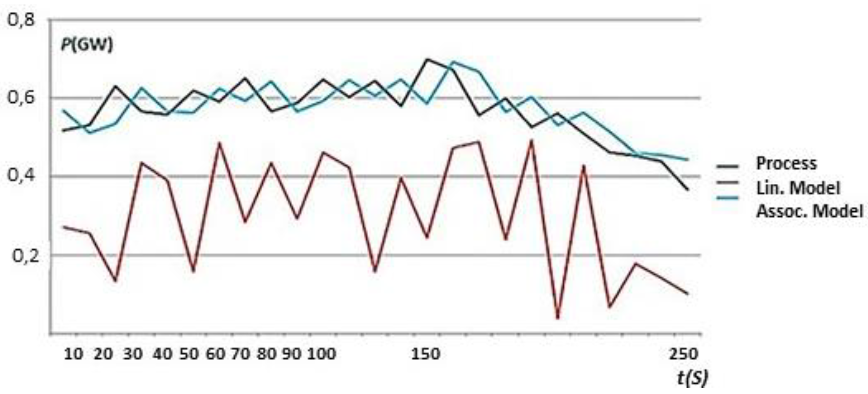
Figure 1 demonstrates power dynamic estimation for a certain facility in the power system.
the black line represents the dynamics of the real process;
the red line shows the result in a linear model;
and the blue line shows the result obtained by associative search model.
Figure 1 shows how a more accurate estimate of a real process dynamics can be obtained using the associative search model, compared with the classical linear models.
7. Conclusions
Predictive bilinear models of discrete dynamical systems are obtained using the associative search algorithm. The method is based on the use of machine learning procedures and inductive knowledge (associative patterns) extraction from historical data. The method features high algorithmic speed, since the main computational load falls on the training stage.
According to the proposed scheme, we, at first, obtain a bilinear model of a nonlinear dynamic object, and then analyze the stability. The advantages of the scheme are the accuracy and speed of the identification algorithm.
Section 6 demonstrates the operation of the associative search algorithm. It shows that for nonlinear systems the models obtained through this algorithm are more accurate as against the ones obtained using traditional linear techniques.
Furthermore, according to our scheme, separable spectral expansions of discrete Lyapunov equations are obtained for MISO LTI discrete dynamical systems governed by state equations in controllability and observability forms. A method and an algorithm for the element-wise solution of the generalized matrix Lyapunov equation are developed for discrete bilinear systems. The new method is a spectral version of the well-known iterative method used for solving this equation.
A sequence of values is calculated for a fixed element of the solution matrix. The element depends on the eigenvalues product of the dynamics matrix of the linear part and the elements of the nonlinearity matrixes. A sufficient condition for the convergence of all sequences is obtained, which is also a BIBO stability condition for a bilinear system.
The article discusses MIMO, MISO, and SISO classes of bilinear systems of the form (10) but does not consider bilinear systems with distributed parameters. In the future, the authors intend to extend the new method over this class of systems. Time-variant systems will be also investigated.


