Abstract
This paper deals with a diffusive predator–prey model with two delays. First, we consider the local bifurcation and global dynamical behavior of the kinetic system, which is a predator–prey model with cooperative hunting and Allee effect. For the model with weak cooperation, we prove the existence of limit cycle, and a loop of heteroclinic orbits connecting two equilibria at a threshold of conversion rate , by investigating stable and unstable manifolds of saddles. When , both species go extinct, and when , there is a separatrix. The species with initial population above the separatrix finally become extinct, and the species with initial population below it can be coexisting, oscillating sustainably, or surviving of the prey only. In the case with strong cooperation, we exhibit the complex dynamics of system, including limit cycle, loop of heteroclinic orbits among three equilibria, and homoclinic cycle with the aid of theoretical analysis or numerical simulation. There may be three stable states coexisting: extinction state, coexistence or sustained oscillation, and the survival of the prey only, and the attraction basin of each state is obtained in the phase plane. Moreover, we find diffusion may induce Turing instability and Turing–Hopf bifurcation, leaving the system with spatially inhomogeneous distribution of the species, coexistence of two different spatial-temporal oscillations. Finally, we consider Hopf and double Hopf bifurcations of the diffusive system induced by two delays: mature delay of the prey and gestation delay of the predator. Normal form analysis indicates that two spatially homogeneous periodic oscillations may coexist by increasing both delays.
1. Introduction
A predator–prey model can be described by the following equations [1]:
where u and v stand for the densities of prey and predator, respectively. represents the per capita prey growth rate in the absence of predators, and is the functional response characterizing predation. d describes the rate of biomass conversion from predation, and m is the death rate of predator. Many kinds of functional response have been proposed [2]. Among them, Holling type I, II, and III [3,4,5,6] are discussed widely, which are prey-dependent functional response.
Cooperative behavior within a species is very common in nature, of which cooperative hunting is the most widely distributed form in animals. In mammals, the most famous examples include wolves [7], African wild dogs [8], lions [9], and chimpanzees [10], who cooperate for hunting preys. Cooperative behaviors are also widespread in other living organisms, such as aquatic organisms [11], spiders [12], birds [13], and ants [14], who find, attack, and move their preys together. Due to hunting cooperation, the attack rate of predators increases with predator density, which obviously depends on both prey and predator densities. Recently, a few literatures have paid attention to derive functional response to describe the cooperative hunting [1,15,16]. Cosner et al. [1] proposed a functional response to explore the effects of predator aggregation when predators encounter a cluster of prey. Berec [15] generalized the Holling type-II functional response to a family of functional responses by considering attack rate and handling time of predators varying with predator density to interpret the foraging facilitation among predators. Alves and Hilker [16] considered a special case of the more general functional response proposed by Berec [15]. They added a cooperation term to the attack rate for representing the benefits that hunting cooperation brings to the predator population, which makes the functional response . Here, describes the strength of predator cooperation in hunting, and is referred to as the cooperation term. They found that cooperative hunting can improve persistence of the predator, and it is a form of foraging facilitation which can induce strong Allee effects. After their work, various types of biological factors (such as Allee effect, fear effect, and so on) and spatial diffusion are incorporated into continuous-time predator–prey models with cooperative hunting [17,18,19,20,21,22]. The impact of hunting cooperation in discrete-time predator–prey models have also been investigated [23,24,25,26]. Pal et al. [23] observed that hunting cooperation can modify the period-doubling route to chaos by reverse period-halving bifurcations and makes the system stable. Chow et al. [26] derived a sufficient condition for which both populations can coexist.
The most well-known example of is the logistic form , where r is the intrinsic growth rate and K denotes the environmental carrying capacity. Then, in the absence of predator, the prey population is governed by . We can conclude from the equation that the species may increase in size when the density is low. However, for many species, low population density may induce many problems, such as mate difficulties, inbreeding, and predator avoidance of defense. It turns out that the growth rate of the low density population is not always positive, and it may be negative when the density of population is less than the minimum number a for the survival of the population, which is called the Allee threshold. The phenomenon is known as the Allee effect, which was first observed by Allee [27], and has been observed on various organisms, such as vertebrates, invertebrates, and plants. Such a population can be described by . The Allee effect may cause the extinction of a low-density population. Because of increasing fragmentation of habitats and invasions of exotic species, the Allee effect has aroused increasing attention (see, for example, in [28,29,30] and the references cited therein).
Jang et al. [17] considered both the cooperation in the predator and Allee effects in the prey, and proposed the following predator–prey model:
where is the per capita intrinsic growth rate of the prey, is the environmental carrying capacity for the prey, () is the Allee threshold of the prey population, is the attack rate per predator and prey, measures the degree of cooperation of predator, is the prey conversion to predator, and is the per capita death rate of predator. They discussed the existence and stability of the equilibria and the occurrence of Hopf bifurcation. They also devised a best strategy for culling the predator by maximizing the prey population and minimizing the predators along with the costs associated with the control.
In fact, the preys and predators distribute inhomogeneously in different locations, and the spatial diffusion plays an important part in the process of population evolution. Turing instability and Turing–Hopf bifurcation induced by diffusion have been widely investigated recently (see in [31,32,33,34]).
It has been widely accepted that time delays have very complex effect on the dynamics of a system, for example, some delays can destroy the stability of equilibria and induce various oscillations and periodic solutions (see, for example, in [35,36,37,38] and references cited therein). There are time delays in almost every process of population interaction, so it is more realistic to introduce time delays when we model the interaction of predator and prey. For example, after consuming the prey, the corresponding biomass cannot be added to the predator population immediately. Thus, the reproduction of predator after predating the prey will be mediated by some discrete time lag (say ) required for gestation of predator, which can be regarded as gestation delay. Therefore, the growth rate of predator depends on the number of individuals present at time . There is an extensive literature about the studies of the dynamics of predator–prey models with the effect of gestation delay of the predator [35,36,37,38]. There is a time lag (say ) in the growth to maturity of the prey, and such a maturation delay of the prey has also been considered [39,40,41,42,43]. However, to the best of our knowledge, there is very little literatures on delayed predator–prey system with Allee effect [44].
Taking into account the diffusion and delays in system (2), we consider the following diffusive system with two delays:
Here, is the time delay due to the maturation of the prey, is time delay due to gestation of the predator, and we define . are the diffusion coefficients characterizing the rates of the spatial dispersion of the prey and predator population, respectively.
Systems with multiple delays have attracted much attention [45,46,47,48,49,50,51]. Generally, delay may induce Hopf bifurcation, and if Hopf bifurcation curves intersect, double Hopf bifurcation may arise. To figure out the effect of delay on the dynamics of systems, Hopf bifurcation and double Hopf bifurcation induced by delay have been investigated [52,53,54,55,56]. However, in most of literatures we mentioned above, the system is reduced into a system with one delay. In fact, systems with multiple delays conform to reality better than one single delay. Recently, the research on the dynamics and bifurcation analysis of system with two simultaneously varying delays are of great interest to scholars. In [49,57], double Hopf bifurcation induced by two delays is studied by different methods. Through the analysis of double Hopf bifurcation, we can classify the topological structures of various bifurcating solutions. By the classification, the dynamics in the neighborhood of the double Hopf bifurcation point in system can be obtained completely.
For the convenience of discussion and reducing the number of parameters, we nondimensionalize the model by letting
Dropping the hats for simplicity of notations, we obtain the simplified dimensionless system
where . Recalling the definition of Allee effect, one always has . In fact, for fixed , , , , and m, we have c and p directly proportional to and , respectively. Thus, we refer to c and p as the degree of cooperative hunting of the predator and the conversion rate from the prey to the predator, respectively, in the context. By the explanation above, we make the following assumption always:
The Allee effect can drive the extinction of low-density species, some of which are preyed by predators that engage in cooperative hunting. This paper investigate the dynamics of system (4) with cooperative hunting and Allee effect from the point of view bifurcation analysis, which can provide useful insights into the intersection of the predator and prey, and help us figure out how to prevent such a prey population from extinction. We find out that the number of constant steady states of (4) is highly dependent on the strength of cooperation in predator c. When , there is one or no positive steady states, while when , there is no, one or two positive steady states. We say the cooperation in the former case is weak, and that in the latter is strong. First of all, we figure out the global dynamical behavior of the kinetic system through the analysis of local bifurcation and the stable and unstable manifolds, taking p as a bifurcation parameter. The existence of some connecting orbits is obtained, thus, a partition of the phase space is given, i.e., the attraction basin of each stability state is obtained. For the model with weak cooperation, we give the condition of the stability of the positive steady state and the occurrence of Hopf bifurcation. Through detailed analysis on the stable and unstable manifolds of saddles, we prove theoretically there is a loop of heteroclinic orbits when . When , the extinction steady state is globally asymptotically stable. When , there is a separatrix, which is the stable manifold of . The orbits above the separatrix converge to , and the orbits below it may converge to , or a limit cycle. Thus, there are three types of bistability: bistability between two boundary equilibria, between a boundary equilibrium and a interior equilibrium, and between a boundary equilibrium and a limit cycle. For the model with strong cooperation, it turns out there are many complex phenomena, including limit cycle, homoclinic cycle, and a loop of heteroclinic orbits between two or among three equilibria. The model may display tristable dynamics, including extinction state, coexistence or sustained oscillation, and the survival of the prey only.
Second, we discuss the diffusive system (4) with no delays. Taking diffusive coefficients as parameters, we give the condition of Turing instability and Turing–Hopf bifurcation in both weak and strong cooperation cases. We discuss the effect of diffusion on the dynamics, and illustrate complex spatio-temporal dynamical behavior, including the existence of spatially inhomogeneous steady state, coexistence of two spatially inhomogeneous periodic solutions.
Third, taking two time delays as bifurcation parameters, we study the effect of two simultaneous varying delays on the dynamics of system (4). After some detailed analysis on the characteristic equation with three exponential terms, the stability switching curves are obtained, on which there is a pair of purely imaginary eigenvalues. An intersection of the stability switching curves may be a double Hopf bifurcation point. We derive the normal form on the center manifold near the double Hopf bifurcation point, and give the unfoldings near the critical points, which indicate that two spatially homogeneous periodic oscillations may coexist by increasing both delays.
The scheme of this paper is arranged as follows. In Section 2, we investigate the existence of constant steady states for system (4). In Section 3, we analyze the local bifurcation and the global dynamics of the kinetic system (7) with weak cooperation and strong cooperation, respectively. In Section 4, we consider the effect of diffusion on system (4) through investigating Turing instability and Turing–Hopf bifurcation. In Section 5, we consider the diffusive system with two delays, and Hopf bifurcation and double Hopf bifurcation induced by two delays are analyzed on the center manifold via normal form approach. In Section 6, we carry out some numerical simulations to support our theoretical analysis and illustrate complex dynamical phenomenon.
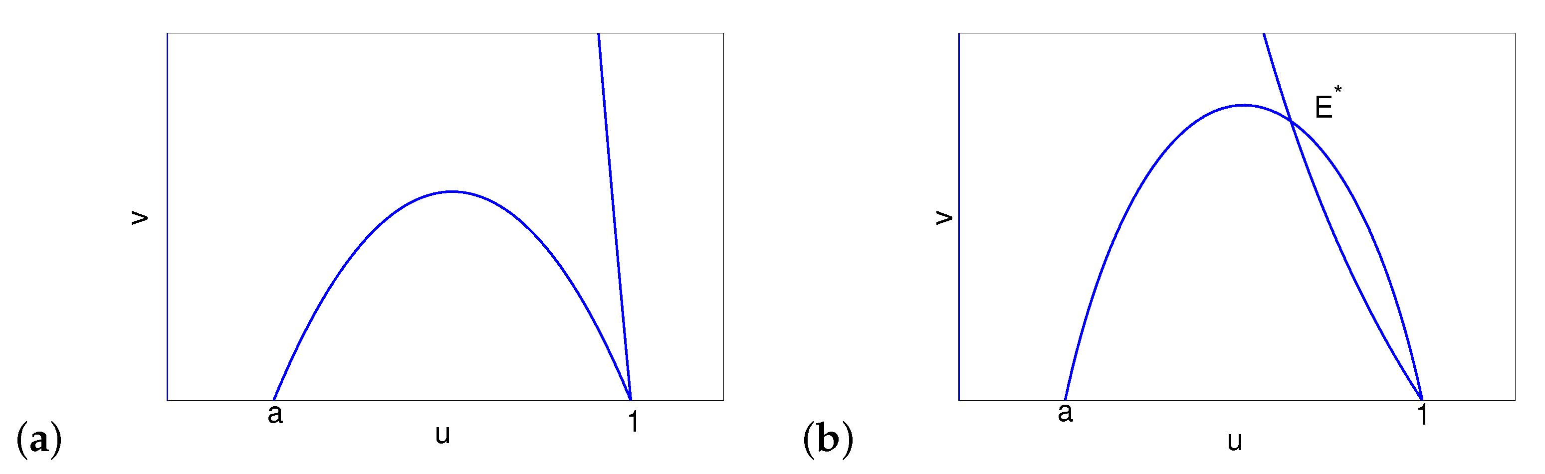
2. The Existence of Constant Steady States
First, we consider the existence of steady states of model (4). As (4) is two-dimensional, it is hard to consider non-constant steady states. Thus, we only discuss the existence of constant steady states.
System (4) has three boundary equilibria: (i) , which means the extinction of both the species; (ii) , which is induced by Allee effect; and (iii) , which means the extinction of the predator and the survival of the prey, achieving its carrying capacity.
Now, we discuss the existence of interior equilibria. Obviously, any interior equilibrium has components and satisfying
i.e.,
In fact, is an ellipse, sitting in the first and forth quadrant, and intersecting the horizontal axis at a and 1. intersects the horizontal axis at , and is decreasing and concave in . Denote the u-nullcline as , and the v-nullcline as . The existence of interior equilibria may have the following different cases.
Proposition 1.
(i) When , system (4) has no interior equilibria.
Proof.
In fact, when , two nullclines have two intersections: in the first quadrant and in the forth quadrant. Thus, there is a unique interior equilibrium with and satisfying (5). When decreases to a, collides with , and is still in the forth quadrant. When , moves into the forth quadrant, leaving no interior equilibria.
When increases to 1, v-nullcline and u-nullcline intersect at , with the slopes of tangents at being and , respectively. If , collides with when , is in the forth quadrant, and there is no interior equilibria (see Figure 1a). Moreover, when , there is no interior equilibria. If , (sitting in the forth quadrant when ) collides with when , and there is a unique interior equilibrium in the first quadrant (see Figure 1b). When and close to 1, moves into the first quadrant, and there are two interior equilibria and . If goes on to decrease, there exists a , such that the u-nullcline and v-nullcline tangent at , where and collide, and there is a unique interior equilibrium . When , there is no interior equilibria. □
Figure 1.
When , (a) there is no interior equilibrium if , and (b) there is one interior equilibrium if .
Remark 1.
In the absence of cooperative hunting within the predator, i.e., , system (4) always has a unique interior equilibrium . The predator and prey coexist if and only if , and the predator is distinct if . However, from proposition 1, the predator and prey still coexist when with strong cooperation, which means that strong cooperation is beneficial for the survival of predator.
Proposition 1 tells us that the strength of cooperation is a threshold for the system (4). To be specific, if , system (4) has at most one coexisting equilibrium, while if , system (4) may have two coexisting equilibria. Thus, in the following discussion, when , we say the cooperation among predators is weak; when , the cooperation is strong.
3. Bifurcation and Global Dynamics of Kinetic System
Before the discussion of the stability of equilibria of system (4), we should first figure out the stability of the equilibria of the kinetic system
We investigate the local bifurcation and global dynamics when the cooperation is weak and strong, i.e., when and .
3.1. Bifurcation and Global Dynamics of Kinetic System with Weak Cooperative Hunting
From proposition 1, if , system (4) has a unique interior equilibrium. In this section, taking p as bifurcation parameter, we first investigate the Hopf bifurcation near the unique interior equilibrium. Through studying the stable manifold and unstable manifold of saddles, we prove the existence of loop of heteroclinic orbits, and get the global dynamics of system (7).
3.1.1. Stability of All Equilibria and Hopf Bifurcation at
The Jacobian matrices of the function on the right-hand of system (7) around , , and are
respectively, from which we can easily get the local stability of the boundary equilibria.
Lemma 1.
For system (7),
- (i)
- is a stable node;
- (ii)
- is an unstable node if , and it is a saddle if ; and
- (iii)
- is a stable node if , and it is a saddle if .
For the interior equilibrium , the corresponding Jacobian matrix is
and thus
In fact, u-nullcline and v-nullcline intersect at , where the slope of is larger than that of , i.e., . Thus, . Thus may be node or focus, and its stability depends on the trace
Thus, we have the following conclusions on the stability of .
Theorem 1.
If , then there exists a unique such that the unique interior equilibrium is locally asymptotically stable when , and unstable when . Moreover, system (7) undergoes a Hopf bifurcation at when .
Proof.
Solving for , when , we obtain a unique , such that on , and on (see Figure 2). Moreover, it is easy to verify that ; thus, corresponding to , we obtain a unique (), such that when , and when .
Figure 2.
The blue curve represents , and the black line represents . When , .
Remark 2.
When there is no cooperative hunting in predator, i.e., , the v-nullcline is , which is vertical. The system undergoes a Hopf bifurcation near when , which is the top of the u-nullcline . In fact, it has been discussed widely that the stability of positive equilibrium can be stated graphically by the u-nullcline when the v-nullcline is vertical: is unstable if the v-nullclines intersect to the left of a local maximum of the u-nullcline, and stable if they intersect to the right [29,58,59,60], and thus, Hopf bifurcation occurs at the “top of the hump” of u-nullcline. However, for system (7) in this paper, the v-nullcline is not vertical, and we can verify that the intersection of the u-nullcline and the v-nullcline corresponding to the Hopf bifurcation point is on the right of the “top of the hump" of u-nullcline. In fact, the “top of the hump” of u-nullcline achieves at , at which the corresponding value of p is denoted by . When , can be also proved to be unstable. Comparing the results in systems with and without cooperation, we can conclude that cooperative hunting is more likely to bring instability into .
In order to determine the direction of Hopf bifurcation and the stability of the Hopf bifurcating periodic solution, we need to calculate the normal form near the Hopf bifurcation point. Through direct calculation following the steps in [61], we can get the following truncated normal form:
Recalling that , the direction of Hopf bifurcation and stability of Hopf bifurcating periodic solution are determined by the first Lyapunov coefficient , and we have the following conclusion.
Theorem 2.
If , system (7) undergoes a Hopf bifurcation at when .
- (i)
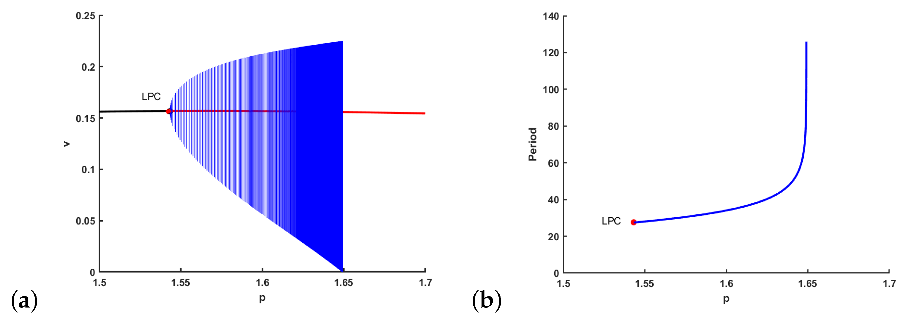
- If , the bifurcating periodic solution is orbitally asymptotically stable, and it is bifurcating from as p increases and passes .
- (ii)
- If , the bifurcating periodic solution is unstable, and it is bifurcating from as p decreases and passes .
3.1.2. The Global Dynamics of Kinetic System with Weak Cooperative Hunting
From the previous discussion, we have known the stability of all equilibria when . Motivated by the work of [29,30], we investigate the global dynamics of system (7). To this end, we should first study the properties of stable manifold of and unstable manifold of , denoted by and , respectively. For the region bounded by and , we prove the existence or nonexistence of periodic orbits. We leave them in Appendix A, and only list main conclusions on the existence of a loop of heteroclinic orbit and global dynamics in the following.
From the monotonicity of S and U given in Proposition A1, we have the following conclusion.
Proposition 2.
If , then there exists a unique , such that , forming a heteroclinic orbit from to .
In fact, there is another heteroclinic orbit from to , which is formed by the unstable manifold of and the stable manifold of on the axis. Thus, there is a loop of heteroclinic orbits from to , and then back to .
Theorem 3.
Suppose that .
- (i)
- If , is globally asymptotically stable (see Figure 3a).
Figure 3. Phase portrait of system (7) for when (a) ; (b) and close to ; (c) and close to 1; (d) and . - (ii)
- There is an such that if , connects to , and the extinction equilibrium is globally asymptotically stable (see Figure 3b).
- (iii)
- There is an such that if , then connects to . The orbits through any point above converge to , and the orbits through any point below converge to (see Figure 3c).
- (iv)
- If , the orbits through any point above converge to , and the orbits through any point below converge to (see Figure 3d).
We leave the proof in Appendix A.2.
Theorem 3 provides a global description of the dynamical behaviour of system (7) for . When , if every periodic orbit of system (7) is orbitally stable, thus there can be at most one such orbit. From Proposition A5, we have the following conclusion.
Theorem 4.
Suppose that , the first Lyapunov coefficient , and every periodic orbit of system (7) is orbitally stable. Then, .
- (i)
- If , connects to . The orbits through any point above converge to , and the orbits through any point below converge to .
- (ii)
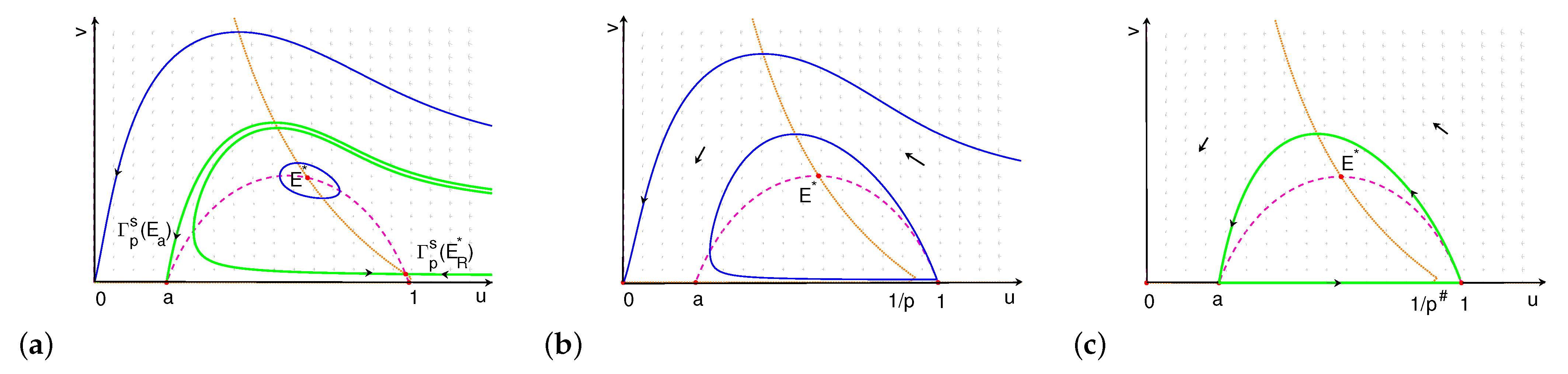
- If , is a repellor, and there is a unique limit cycle under . The orbits through any point below converge to the limit cycle. (see Figure 4a,b).
Figure 4. Phase portrait of (7) for when (a) and close to ; (b) and close to ; (c) ; (d) . - (iii)
- If , , there are two heteroclinic orbits forming a loop of heteroclinic orbits from to and back to (see Figure 4c). The orbits through any point exterior to the loop converge to , and the orbits through any point interior to the cycle converge to the loop.
- (iv)
- If , connects to , and the extinction equilibrium is globally asymptotically stable (see Figure 4d).
Remark 3.
We leave the proof in Appendix A.3.
From the former conclusion on the global dynamics of model (7) with weak cooperation, we find that no matter how we choose the value of p, both of the two species are extinct if the ratio of predator to prey is high.
Now, we discuss the population behavior when the ratio of predator to prey is low. When , because of the low conversion rate, the predator is extinct, while the prey reach the capacity of the environment. When , the predator and prey coexist, and tend to a constant value. When , the predator and prey coexist, but oscillate sustainably. The amplitude of oscillation increases as p increases, and the minimum of the predator population is close to zero when p is close to , which will increase of risk on the extinction of predator. When the value of p is too high, high growth rate of prey leads to over hunting, and finally, both of the two species are extinct.
Remark 4.
Similar to the case in the model with Allee effect, there is a unique positive equilibrium in the model without Allee effect, and the varying p makes unstable and induces Hopf bifurcation. However, there is an additional saddle point in the model with Allee effect, and the stable manifold of the saddle point separates the positive quadrant into two positive invariant regions. If the initial populations are above the stable manifold of , extinction happens for both species in the model with Allee effect, while coexistence happens for the model without Allee effect. This extinction is mediated by too high predator density that drives the prey density below the Allee threshold and both species become extinct.
3.2. Bifurcation and Global Dynamics of Kinetic System with Strong Cooperative Hunting
By strong cooperation we mean . In this section, we first analyze the stability of interior equilibrium, then we prove the existence of Hopf bifurcation and give the condition of the existence and nonexistence of loop of heteroclinic orbits. We also exhibit the complex dynamics of model (7), such as limit cycle, loop of heteroclinic orbits, and homoclinic cycle.
3.2.1. Stability and Hopf Bifurcation of Interior Equilibria
Now, we consider the stability of interior equilibria. For or , the corresponding Jacobian matrix is
and thus
If , then , which means that is tangent to . In fact, the point of tangency is , thus . It is clear that for , and for (see Figure 5). The component of is always satisfying , and the component of is satisfying (see Figure 1). It follows that for , , while for , . Thus, exists when , and it is a saddle. exists when , and . Thus, may be node or focus, and its stability depends on the trace
Figure 5.
The red curve represents the figure of , and the green straight line represents .
Similar as the proof in Theorem 1, solving for , when , there is a unique such that on , and on (see Figure 2). Recalling that , corresponding to , we obtain a unique (), such that when , and when .
Let be the roots of when p is near . We can prove , in a similar way as in Theorem 1. Therefore, we can get the following theorem.
Theorem 5.
When , there exists a unique such that is locally asymptotically stable if , and unstable if . Moreover, system (7) undergoes a Hopf bifurcation at when .
3.2.2. The Global Dynamics of Kinetic System with Strong Cooperative Hunting
When , system (7) may have one or two interior equilibria, which brings a few complications to the dynamics of model (7). There are three different cases of global dynamics when c takes different sizes. In this section, we exhibit the dynamics combining theoretical analysis and numerical simulations.
First, we consider the properties of the stable manifold of , unstable manifold of , as well as stable and unstable manifold of , which are in Appendix B. Then, we can determine the global dynamics of model (7) when p is chosen in the following ranges. As in Theorem 3, we can prove the following conclusion.
Theorem 6.
Suppose that .
- (i)
- If , is globally asymptotically stable (see Figure 6a).
Figure 6. If , phase portrait of (7) when (a) ; (b) and close to ; and (c) . - (ii)
- If and near , connects to , and the extinction equilibrium is globally asymptotically stable (see Figure 6b).
- (iii)
- If , the orbits through any point above converge to , and the orbits through any point below converge to (see Figure 6c).
The remaining question is how are the dynamics of system (7) for p chosen in the rest ranges, i.e., . As larger c means less steep of the v-nullcline, the critical points (for example, , ) may appear in different ranges, and there are the following three different cases.
Case 1 Choose suitable c such that , , and . From Theorem A1, there is a loop of heteroclinic orbits when . We have the following conclusion.
Theorem 7.
Suppose that , , and . Assume that the first Lyapunov coefficient , and every periodic orbit of system (7) is orbitally stable, then .
- (i)
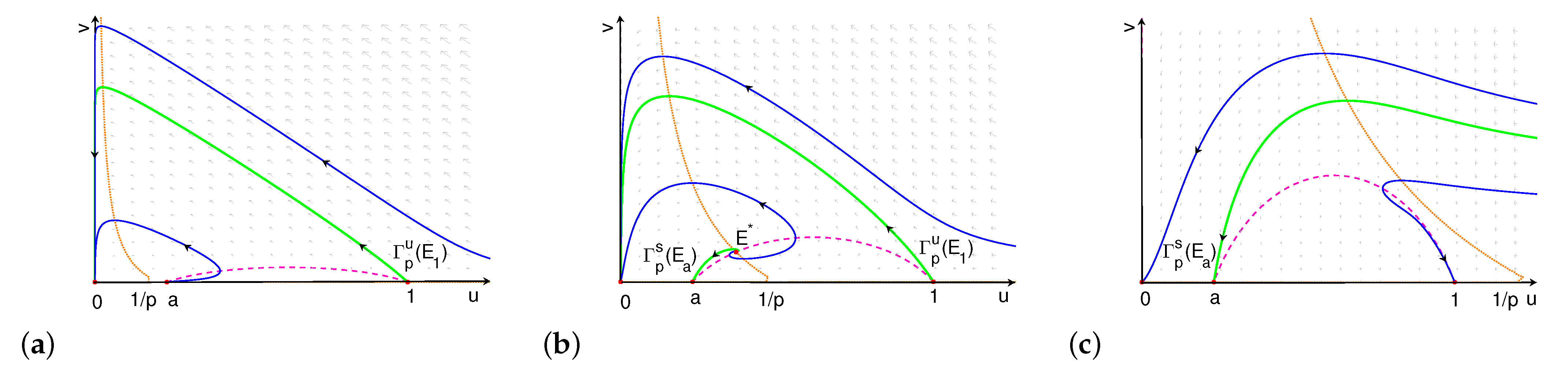
- If , the upward connects to . The orbits through any point above converge to , and the orbits through any point inside the stable manifold converge to . The orbits through any point below and exterior to converge to (see Figure 7a).
Figure 7. Phase portrait of system (7) for case 1 when (a) and close to , (b) and close to , (c) and close to , and (d) . - (ii)
- If , connects to . The orbits through any point above converge to , and the orbits through any point below converge to .
- (iii)
- When , is a repellor, and there is a unique limit cycle under . The orbits through any point below converge to the limit cycle (see Figure 7b,c).
- (iv)
- When , , and there are two heteroclinic orbits forming a loop of heteroclinic orbits between and (see Figure 7d). The orbits through any point exterior to the cycle converge to , and the orbits through any point interior to the cycle converge to the cycle.
- (v)
- If , connects to , and the extinction equilibrium is globally asymptotically stable (phase portrait is similar as Figure 6b).
Proof.
From Proposition A6, is decreasing with p, combining with , then enters from the region for all . As is stable when , then is stable for all . If there is a periodic orbit below , it must encircle , and it is unstable from inside, which contradicts with our assumption of the orbital stability of periodic orbit. It means that there is no periodic orbit under for all . From Proposition A9, is the limit set of , and must be above . The upward connects to (see Figure 7a). Thus, the orbits through any point inside the stable manifold converge to . The proof of (ii)–(v) is similar as that of Theorem 4. □
Case 2 Choose suitable c such that , , and . From Theorem A1, there is a loop of heteroclinic orbits when .
Theorem 8.
Choose suitable c such that , , and . Assume that the first Lyapunov coefficient , and every periodic orbit of system (7) is orbitally stable, then .
- (i)
- If , the upward connects to , and the downward connects to . The orbits through any point above converge to , and the orbits through any point inside the stable manifold converge to . The orbits through any point below and exterior to converge to (phase portrait is similar as Figure 7a).
- (ii)
- When , there is a unique limit cycle inside the stable manifold of (see Figure 8a). The orbits through any point interior to converge to the limit cycle.
Figure 8. Phase portrait of system (7) for case 2 when (a) and close to ; (b) and close to ; (c) . - (iii)
- When , there is a unique limit cycle under . The orbits through any point below converge to the limit cycle (see Figure 8b).
- (iv)
- When , , there are two heteroclinic orbits forming a loop of heteroclinic orbits from to and back to (see Figure 8c). The orbits through any point exterior to the cycle converge to , and the orbits through any point interior to the cycle converge to the cycle.
- (v)
- If , connects to , and the extinction equilibrium is globally asymptotically stable (phase portrait is similar as Figure 6b).
Proof.
We can prove (i) similar as in Theorem 7. (ii) As and , there is a stable periodic orbit bifurcating from Hopf bifurcation when . As in the proof of Theorem 7, we can prove that must be above . From Proposition A9, the unique limit cycle is the limit set of . The proof of (iii)–(v) is similar as that of Theorem 4. □
Case 3 Choose c such that and . From Theorem A1, there is no heteroclinic orbits from to . It is easy to prove that when , is globally asymptotically stable (see Figure 9e).
Figure 9.
Phase portrait of system (7) for case 3 when (a) and near , there is a limit cycle inside the stable manifold of ; (b) and near , there is a limit cycle inside the stable manifold of ; (c) , the upward unstable manifold and the left stable manifold of collide, which forms a homoclinic cycle; (d) the upward unstable manifold of , the unstable manifold of on the axis, and the downward unstable manifold of forms a loop of heteroclinic orbits among , , and when ; and (e) .
Remark 5.
In this case, the location of , and are very complicated. We can observe the following dynamics by numerical simulations.
- (i)
- Loop of heteroclinic orbits. The downward branch of the unstable manifold of connects to , and the upward connects to , which collides with the the stable manifold of . The upward and downward unstable manifold of , together with the unstable manifold of on the axis, forms a loop of heteroclinic orbits among , and when (see Figure 9d).
- (ii)
- Homoclinic cycle. The upward unstable manifold and the left stable manifold of collide, which forms a homoclinic cycle. Denote the parameter p as (see Figure 9c).
- (iii)
- Limit cycle induced by Hopf bifurcation (see Figure 9a,b).
Remark 6.
There are two positive equilibria and in both of the model with or without Allee effect, where is always a saddle. In the model without Allee effect, the stable manifold of separates the positive quadrant into two positive invariant regions. Two species coexist if the initial populations are above the stable manifold. However, there is an additional stable manifold of saddle point in the model with Allee effect, and two stable manifolds of the two saddle points separate the positive quadrant into three positive invariant regions. Two species only coexist between the two stable manifolds, and both species go extinct if the initial populations is above the stable manifold of . This means that the region of coexistence of two species is reduced due to the Allee effect.
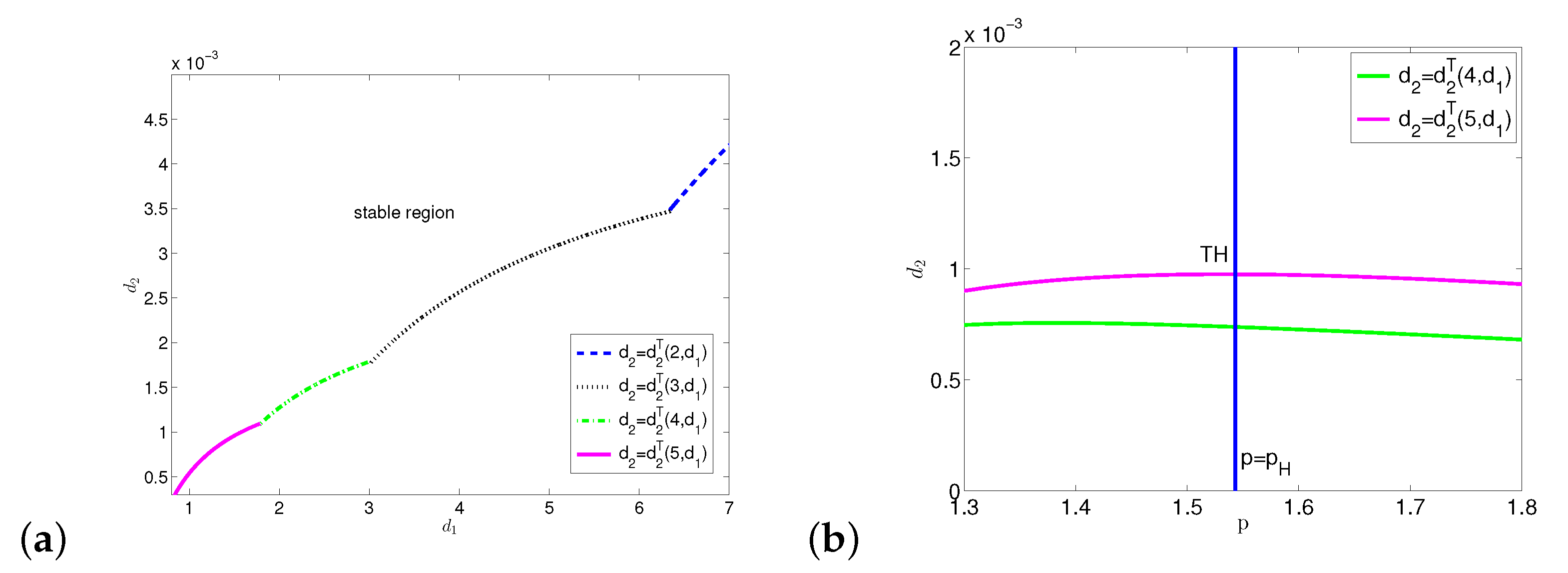
4. Diffusion-Driven Turing Instability and Turing–Hopf Bifurcation
In the previous section, we have discussed both local bifurcation and global dynamics of kinetic model (7). In this section, we consider the effect of the diffusion on the stability of the interior constant steady states; thus, we set in system (4). If an equilibrium is linearly stable in the absence of diffusion, and it becomes unstable in the presence of diffusion, we call such an instability Turing instability. As is always a saddle if it exists, thus Turing instability can only happen near in both cases: weak cooperation and strong cooperation. We first investigate the existence of Turing instability, then we consider Turing–Hopf bifurcation near .
For Neumann boundary condition, we define the real-valued Sobolev space
It is well known that the eigenvalues of on X are and , . From straightforward calculation, we obtain the characteristic equations
where
From the previous section, in the absence of diffusion, i.e., , is asymptotically stable if in the case of (if in the case of ). If there exists an , such that has roots with positive real part when , Turing instability occurs. As when , and always satisfies, from (15), we have for any n when . Therefore, when , the signs of the real parts of roots of (14) are determined by the signs of .
In fact, the curve of is a hyperbola on plane, whose horizontal and vertical asymptotes are and . We only need to consider the right branch of the hyperbola, which intersects with the axis at . Thus, with respect to n, both the horizontal asymptote of the right branch of the hyperbola and the intersection with the axis are decreasing.
Denote
Noting that when , we have if , and if .
Theorem 9.
If , suppose (If , suppose ). The constant steady state is locally asymptotically stable if for all , while it is Turing unstable if for some satisfying .
On the plane, we call the boundary curve of stable region of steady state the Turing bifurcation curve , which is formed by a sequence of curve segments
where is the intersection of and , and can be infinite.
When , for all , similar as the analysis in the case of , we can also get a Turing bifurcation curve, and we have the following conclusion.
Remark 7.
Assume, in the plane, and intersect at a point , then the characteristic equation has a pair of purely imaginary roots and a zero root at . According to the general theory of [62], a Turing–Hopf bifurcation may appear. However, rigorous derivation for the normal form is impossible due to the implicit form of in this paper. We shall give some numerical illustrations to show the dynamics of the system near the Turing–Hopf bifurcation point.
5. The Dynamics of Diffusive System with Two Delays
In the previous section, we have found the conditions of stability and Turing instability of constant steady state of system (4) when . We know that if and for all , the steady state is locally asymptotically stable. In this section, we investigate the diffusive system (4) under the assumption and , and focus on the effect of two delays on the dynamics of the diffusive system near .
5.1. Hopf and Double Hopf Bifurcation Induced by Two Delays
In this subsection, we investigate the existence of Hopf bifurcation induced by two delays by the method of stability switching curves given in [63], and give the condition of the existence of double Hopf bifurcation.
The linearization of system (4) at the steady state is given by
where
and satisfy the homogeneous Neumann boundary condition.
From Wu [64], the corresponding characteristic equation of (18) is
where I is a identity matrix, , . Equation (20) can be written in the following form:
where
The characteristic equation with the form of (21) has been investigated by Lin and Wang [63]. They derived an explicit expression for the stability switching curves, on which there is a pair of purely imaginary roots for (21). Moreover, they gave a criterion to determine the crossing directions, i.e., on which side of the stability switching curve there are two more characteristic roots with positive real parts. Using this method, we can find all the stability switching curves in the plane and determine the crossing directions. We leave the details in Appendix C and Appendix D.
Moreover, we have the following Hopf bifurcation theorem with two parameters.
Theorem 10.
For each , , defined by (A9), is a Hopf bifurcation curve in the following sense: for any and for any smooth curve Γ intersecting with transversely at p, we define the tangent of Γ at p by . If , and the other eigenvalues of (21) at p have non-zero real parts, then system (4) undergoes a Hopf bifurcation at p when parameters cross at p along Γ.
The theorem can be proved by a similar method in [49].
Remark 8.
Suppose that and intersect at a point , with the corresponding values of ω being and . Then, there are two pairs of purely imaginary roots of (21) at the intersection, which are and , denoted by and for convenience. Thus, system (4) may undergo double Hopf bifurcations at the intersection of two stability switching curves near the constant steady state .
5.2. Normal Form on the Center Manifold for Double Hopf Bifurcation
In this subsection, applying the normal form method of partial functional differential equations [65], we derive normal form of double Hopf bifurcation taking two delays as bifurcation parameters. Then, we can classify the topological structures of various bifurcating solutions, and get the dynamics in the neighborhood of the double Hopf bifurcation point in system (4).
For the real-valued Sobolev space X defined in (12), define the complexification space of the real-valued Hilbert space X by
with the general complex-value inner product
Let denote the phase space with the sup norm, and write for , .
Without loss of generality, we assume in this section. Denote the double Hopf bifurcation point by . Let , and set and as two bifurcation parameters. Drop the bars, and denote , then system (4) can be written as
where
with and being defined in (19), and
Consider the linearized system of (23)
We know that the normalized eigenfunctions of on X corresponding to the eigenvalues and ( ) are
respectively, where . Define , satisfying . Denote
System (25) can be rewritten as an abstract ordinary differential equation on [65]
where is the infinitesimal generator of the -semigroup of solution maps of the linear equation (23), defined by
with , and is given by for and . Clearly,
Then, on , the linear equation
is equivalent to the retarded functional differential equation on :
By the Riesz representation theorem, there exists a matrix whose components are bounded variation functions such that
Let () denote the infinitesimal generator of the semigroup generated by (28), and denotes the formal adjoint of under the bilinear form
The calculations of normal form are very long, so we leave them in supplementary materials. Based on the derivation in the Supplementary Materials, the normal form truncated to the third order on the center manifold for double Hopf bifurcation is obtained. Making the polar coordinate transformation, then we obtain the following system corresponding to the truncated normal form
where
and and are the coefficients of the normal form obtained in Supplementary Materials. From Chapter 7.5 in [62], there are twelve distinct kinds of unfoldings for (29).
6. Numerical Simulations
In this section, we carry out some numerical simulations for the kinetic system (7), diffusive system without delays, and the diffusive system (4) with two delays, respectively. These numerical simulations confirm and illustrate our main theoretical results.
6.1. Numerical Simulations for Kinetic System
In this subsection, we carry out some numerical simulations for system (7). We fix the parameters as
6.1.1. Numerical Simulations for Kinetic System with Weak Cooperative Hunting
For system (7), choose such that . To show the complex dynamics of system (7), different values of p are chosen, listed in Table 1 and Table 2. The corresponding phase portraits for different values of p have been illustrated in Figure 3 and Figure 4, which is drawn by pplane8 [66].
Using the method in [67], we can get Hopf bifurcation point , and the first Lyapunov coefficient is , which means that the bifurcating periodic solution is asymptotically stable, and it is bifurcating from as p increases past from Theorem 2. We can draw the bifurcation diagram in Figure 10. If , is asymptotically stable (the black curve in Figure 10a). The increase of p induces instability to . When , becomes unstable (the red curve in Figure 10a), and a unique limit cycle appears (marked by LPC). The period of limit cycle is increasing as p increases from , which tends to infinite as (see Figure 10b). When , the limit cycle coincides with a loop of heteroclinic orbits. When , the loop of heteroclinic orbits breaks and the limit cycle disappears. The corresponding phase portrait has been drawn in Figure 4, and the results are consistent with Theorem 4. Moreover, the amplitude of oscillation increases as p increases, and the minimum of the predator population is close to zero when p is close to , which will increase the risk on the extinction of predator.
Figure 10.
The bifurcation diagram with , and , and the conversion rate p as the bifurcation parameter. (a) The black curve is the stable steady state and the red curve is the unstable steady state. The blue curves denote the amplitude of the limit cycle, which begin at the Hopf bifurcation point . (b) The period of the limit cycles.
6.1.2. Numerical Simulations for Kinetic System with Strong Cooperative Hunting
In Section 3.2, we discuss three different cases of dynamics when c is chosen as different values. To show case 1, we fix and vary p as a bifurcation parameter. We get , and the first Lyapunov coefficient is . Choosing different values of p listed in Table 3, we have drawn the corresponding phase portraits for different values of p in Figure 7.
Table 3.
Values of parameter p chosen for showing case 3 in Figure 9.
To show case 2, choosing and varying p, we can get , and the first Lyapunov coefficient is . Choosing p as listed in Table 2, the corresponding phase portraits have been illustrated in Figure 8.
To show case 3, choosing and varying p, we can get , , and the first Lyapunov coefficient is . We can draw the bifurcation diagram in Figure 11. When (i.e., on the left of LP), there is no interior equilibria. When (i.e., on the right of LP), there are two equilibria (the black curve) and (the blue dotted curve). If , is asymptotically stable (the blue curve). The increase of p induces instability to . When , becomes unstable (the red curve), and a unique limit cycle appears (marked by LPC in Figure 11a). When p increasing from , the period of limit cycle is increasing, and it tends to infinite as (see Figure 11b). Moreover, the amplitude of oscillation increases as p increases, and the amplitude line touches the curve of value of . It means that there is a cycle goes through , which forms a homoclinic cycle. The limit cycle coincides with a homoclinic cycle when . When , the homoclinic cycle breaks, and the limit cycle disappears. Choosing p as listed in Table 3, the corresponding phase portraits have been illustrated in Figure 9.
Figure 11.
The bifurcation diagram with , and , and the conversion rate p as the bifurcation parameter. (a) The black curve is the stable steady state , the red curve is the unstable steady state , and the dotted blue curve is the unstable steady state . The blue curves denote the amplitude of the limit cycle, which begin at the Hopf bifurcation point . (b) The period of the limit cycles.
6.2. Numerical Simulations for Diffusive System without Delays
In this section, we carry out some numerical simulations for diffusive system (4) with . We fix the parameters as
To illustrate the dynamics of (4) with no delays in the case of weak cooperation, we choose such that . Let , from the previous section, is stable when . On plane, we can draw curves determined by (16) for , and we only illustrate four curves for . Correspondingly, from (17), we can get four curve segments, forming partial Turing bifurcation curve (see Figure 12a). From Theorem 9, if we choose and in the region above the curve, the constant steady state is stable. If we choose and in the region under , the steady state of the diffusive system is Turing unstable, and there is a spatially inhomogeneous steady state (see Figure 13).
Figure 12.
(a) Partial Turing bifurcation curve of system (4) with no delays with the parameters . (b) When , the Turing bifurcation curve intersects line at , which is a Turing–Hopf bifurcation point.
Figure 13.
(a) The prey pattern and (b) the predator pattern for system (4) without delays with the parameters . The patterns indicate instability induced by diffusion for the prey and predator. Initial conditions are , .
If we fix , from (16), we can draw Turing bifurcation curve on plane (see Figure 12b), and intersects line at . Choosing near , two stable spatially inhomogeneous periodic solutions coexist when we choose two different initial values (see Figure 14).
Figure 14.
Two spatially inhomogeneous periodic solutions coexist when we choose , , , , , and in system (4) without delays. Initial conditions are , for (a,b), and , for (c,d).
To illustrate the dynamics of (4) without delays in the case of strong cooperation, we choose such that . Let . From (16) and (17), we can draw partial Turing bifurcation curve on plane (see Figure 15a). The constant steady state is stable when we choose and in the region above .
Figure 15.
(a) Partial Turing bifurcation curve of system (4) without delays with the parameters . (b) When , Turing bifurcation curve intersects line at , which is a Turing–Hopf bifurcation point.
If we choose and in the region below , from Theorem 9, the steady state of the diffusive system is Turing unstable. If we fix , from (16), we can draw Turing bifurcation curve on plane (see Figure 15b), and intersects line at . Choosing near , we can illustrate two stable spatially inhomogeneous periodic solutions coexisting when we choose two different initial values (see Figure 16).
Figure 16.
Two stable spatially inhomogeneous periodic solutions of system (4) without delays coexist with , , , , , and . Initial values are , for (a,b), and , for (c,d).
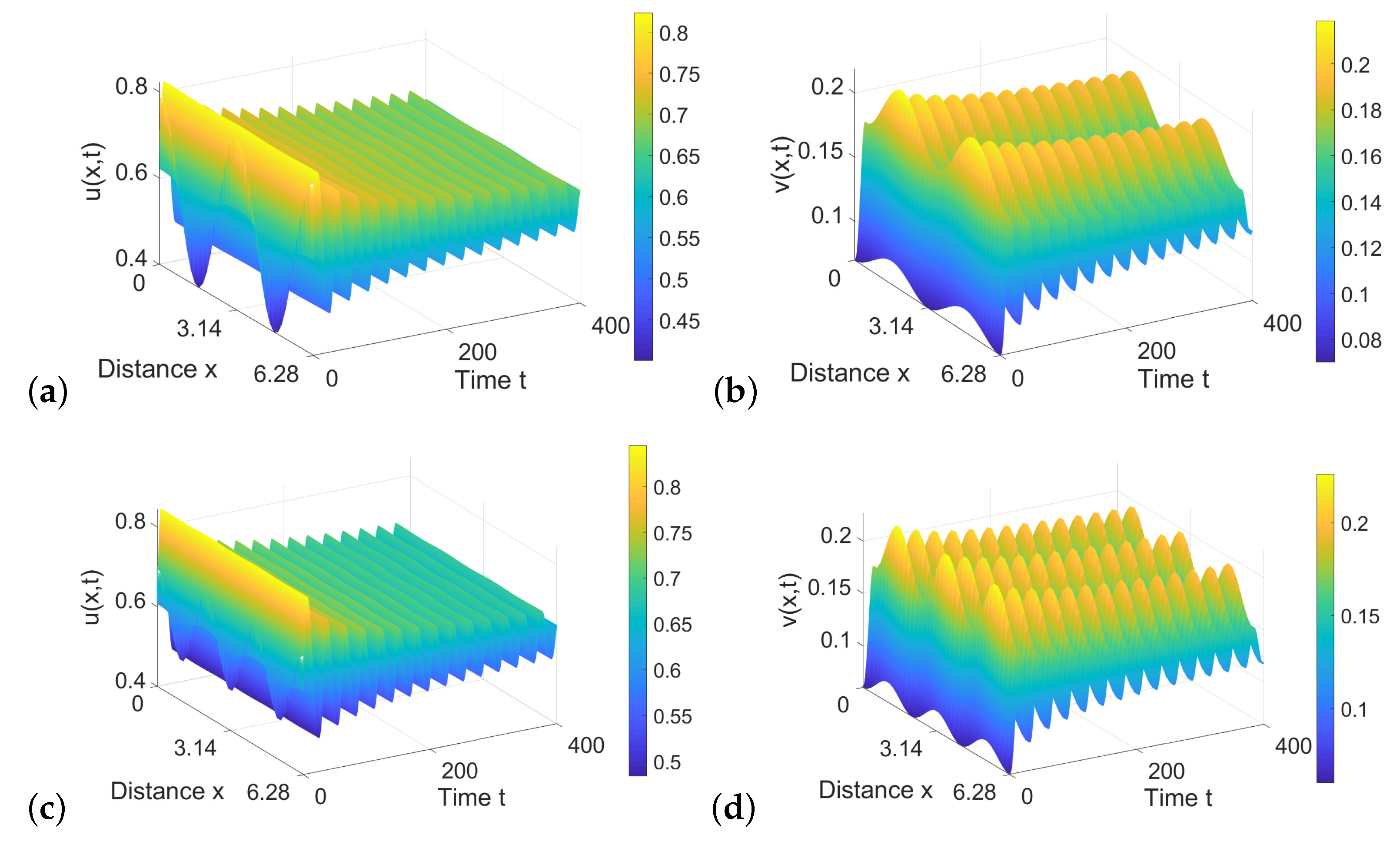
6.3. Numerical Simulations for Diffusive System with Two Delays
In this section, we carry out some numerical simulations for diffusive system (4). Fix
which is the same as in (31). Fix such that , and choose , , and , such that for all . From Theorem 9, one can get the unique constant steady state is locally asymptotically stable.
Now, we illustrate the effect of two delays on the dynamics (4). Following the steps in Appendix C and Appendix D, we can draw all the stability switching curves on plane, and decide the crossing direction, which are shown in Figure A3, Figure A4, Figure A5, Figure A6, Figure A7 in Appendix E. Combining all the stability switching curves together, and zooming in the part of , we get the Hopf bifurcation curves shown in Figure 17a. Consider the bottom left region bounded by left-most curve of and the lowest curve of (see Figure 17a), which are both part of . The crossing directions of the two switching curves (the black line and blue line) are all pointing outside of the region. From Theorem 9, under the assumption and , is locally asymptotically stable. From Theorem 10, when cross from the left to the right of the stability switching curve (or cross from the bottom to the top of ), the characteristic equation has two more characteristic roots with positive real parts from Lemma A1, becomes unstable, and periodic solution occurs due to Hopf bifurcation. Similarly, when cross from the left to the right of stability switching curve (or from the left to the right of stability switching curve ), the characteristic equation has two more characteristic roots. Then, is still unstable, and system (4) undergoes Hopf bifurcation and periodic solution arises. However, the periodic solution is unstable, as there is unstable manifold. It means that stability switching curves and are the boundary of stable region for . In the stable region in Figure 17a, the predator and the prey coexist, and when cross the stability switching curves (or ), the species coexist in the form of sustained fluctuation. From the previous discussion, if we choose a point (2.31, 0) on axis and move up, system (4) undergoes stability switches at . There are two intersections with the boundary of the stable region: , (see Figure 17a). The positive equilibrium is unstable when and there are periodic solutions; becomes locally asymptotically stable and periodic solutions disappear when , and loses its stability when and periodic solution appears again. Multiple times stability switching means that the stability of can switch with the varying of parameters , and periodic solutions may appear or disappear during the stability switching of .
Figure 17.
(a) The left-most curve and the lowest curve of intersect at , which is a double Hopf bifurcation point on the plane. Crossing directions are marked by arrows. (b) The complete bifurcation sets near double Hopf bifurcation point HH.
Moreover, the two stability switching curves intersect at the point , which is the double Hopf bifurcation point, denoted by HH. For HH, , . Using the normal form derivation process given in Supplementary Materials, we have , , , , , , , . Furthermore, we have the normal form (29) with , and . According to Chapter 7.5 in [62], case Ib arises, and we have the bifurcation set near HH showing in Figure 17b. In region , the positive equilibrium is asymptotically stable. In region or , there is a stable periodic solution. When the parameters cross into the region D4, there are two stable homogeneous periodic solutions coexisting in D4.
7. Concluding Remarks
We investigate the dynamics of a diffusive predator–prey model with two delays. First, we discuss the existence of constant coexisting steady states of system (4). It turns out that the strength of cooperation is a threshold: if , i.e., the cooperation is weak, there is at most one coexisting steady state, and if , i.e., the cooperation is strong, there are at most two coexisting steady states.
To figure out the dynamics of system (4), we first carry out the study on the kinetic predator–prey model (7) with Allee effect in prey and cooperative hunting in predators. Compared with the work of Jang et al. [17], which mainly gives the local bifurcation analysis, we mainly focus on the global dynamics. We start with the kinetic system in the case of weak cooperation. Taking p, the conversion rate, as the bifurcation parameter, we prove that there is a loop of heteroclinic orbits between and formed by the intersection of the stable manifold of and the unstable manifold of when (). It shows that is an important threshold, which distinguishes the globally stability for and the existence of a separatrix curve. To be specific, when , is globally stable, which means the extinction of both species, and we call the phenomenon overexploitation. When , there is a separatrix curve , which is determined by the stable manifold of . High initial predator density will lead to extinction for both species, and conversely low initial predator density will approach either a steady state or a periodic oscillation. When , is locally stable, which means that the prey achieves its carrying capacity and the predator is extinct. When , the stable state becomes , which implies the coexistence of both species. When p crosses , the stable state switches into a limit cycle. The period of the limit cycle increases with p, and tends to ∞ as . The existence of a limit cycle with a large amplitude increases the risk of the extinction for the predator.
In the case of strong cooperation, three different cases are considered. We prove the existence of a loop of heteroclinic orbits between and when in the first and second cases and nonexistence of such a loop of heteroclinic orbits in the third case. We also exhibit the existence of loop of heteroclinic orbits among , , and formed by the unstable manifold of and the unstable manifold when , and a homoclinic cycle when by numerical simulations in case 3. When in case 1 and case 2 ( in case 3), both species are distinct. When in case 1 and case 2, there is a separatrix curve , and there are two stable states coexisting, which are extinction for both species and coexistence or oscillation. When (or ) and , there are two separatrix curves, the stable manifold of and the stable manifold of , separating the first quadrant into three parts. If the initial population is above the stable manifold of , both species are extinct; if the initial population is inside the stable manifold of , the stable state can be or limit cycle; if the initial population is below the stable manifold of and outside the stable manifold of the stable manifold of , the prey achieves its carrying capacity and the predator is extinct. When , there is one separatrix curve , and there are two stable states coexisting. The species with initial population above the separatrix finally become extinct, however only the prey survive when initial population is below it.
There is a unique equilibrium for weak cooperation when . It is shown that there are at most two stable states coexist for different initial values separated by the stable manifold of . There are two interior equilibria and in the case of strong cooperation when . The equilibrium brings one more separatrix curve than the case of weak cooperation, thus there may be three stable states coexisting.
Second, we consider the diffusive system without delays, and focus on the effect of diffusion on the dynamics. Taking diffusion coefficients and as bifurcation parameters, we give the conditions of existence of Turing instability and Turing–Hopf bifurcation for the system with both weak and strong cooperation. We illustrate complex dynamics of the diffusive system, including the existence of spatially inhomogeneous steady state, coexistence of two spatially inhomogeneous periodic solutions.
Finally, we discuss the joint effect of two delays on the dynamical behavior of the diffusive system. Applying the method of stability switching curves, we find all the stability switching curves at which the characteristic roots are purely imaginary. Combining the geometrical and analytic method, we can decide the crossing direction of the characteristic roots as long as we confirm the positive direction for stability switching curves. Then, we can get the condition of existence of Hopf bifurcation. By searching the intersection of stability switching curves near the stable region, we get the double Hopf bifurcation point. Through the calculation of normal form of the system, we get the corresponding unfolding system and the bifurcation set, from which we can figure out the complete dynamics near the bifurcation point on the parametric plane. We theoretically prove and illustrate that near the bifurcation point, there are the phenomena of the stability of positive equilibrium: stable periodic solutions and the coexistence of two periodic solutions. From double Hopf bifurcation analysis, we can gain an insight into the local dynamics near the double Hopf bifurcation point. However, numerical simulations tells us that the occurrence of complex phenomena near bifurcation point is sensitive to the choice of initial values. When we choose the initial values with high ratio of predator to prey, both species are extinct. Thus, the complex phenomena near the double Hopf bifurcation probably accompany with an extinction steady state, which is consistent with the results in the kinetic system. Therefore, the analysis of global dynamics of kinetic system can help us comprehend these bistable dynamics for the diffusive system.
Supplementary Materials
The following are available at https://www.mdpi.com/article/10.3390/math9243193/s1, in the Supplementary Material. We give the detailed calculation process of normal forms near double Hopf bifurcation induced by two delays.
Author Contributions
Writing—original draft preparation, Y.D.; writing—review and editing, funding acquisition, Y.D., B.N., and J.W.; methodology, supervision, B.N. and J.W. All authors have read and agreed to the published version of the manuscript.
Funding
This research is supported by National Natural Science Foundation of China (No.11901369, No. 61872227, No.11971281 and No.11771109), Natural Science Basic Research Plan in Shaanxi Province of China (grant No.2020JQ-699) and Shandong Provincial Natural Science Foundation (No.ZR2019QA020).
Institutional Review Board Statement
Not applicable.
Informed Consent Statement
Not applicable.
Data Availability Statement
Not applicable.
Conflicts of Interest
The authors declare no conflict of interest.
Appendix A. Some Results and Proofs for the Case of Weak Cooperation
Appendix A.1. The Properties of Stable and Unstable Manifold and the Existence or Nonexistence of Periodic Orbits
Proposition A1.
Suppose that , and .
- (i)
- The orbit meets the v-nullcline at a point , where , and is a monotone decreasing function for .
- (ii)
- The orbit meets the v-nullcline at a point , where , and is a monotone increasing function for .
Proof.
Inspired by the authors of [29], we prove (i), and the proof for (ii) is similar.
When , is a saddle. The eigenvector corresponding to is , which means that the unstable manifold of is on the u-axis. For , the corresponding eigenvector is . Thus, the tangent vector of the stable manifold of (denoted by ) at is . Comparing with the tangent vector of at , we have , thus is above the nullcline near . Moreover, from the vector field in (7) on , is always above before meets the v-nullcline.
In order to show that meets the v-nullcline, we still need to prove that it remains bounded for . In fact, for , is the graph of a function , satisfying
If there is a such that as , then is bounded below for and any . Thus, for ,
for some positive constant A. It means that is bounded as , which is a contradiction. Thus it cannot blow up before it extends to the v-nullcline . Therefore, exists for all and .
Notice that only when as , which means must be an unstable node. When , is locally stable, thus if . When and near , is an unstable spiral. Thus, the set is a nonempty open set containing .
Now we show that is monotonically decreasing on any component of K. Let be two points in some interval in K. Denote the v-nullcline for and as and . From the expression of , we know that the curve of is on the right of . The stable manifold of for and are graphs of function and defined for , respectively. The corresponding eigenvectors at are , , respectively. Therefore, for u sufficiently near a. Suppose that for some u with . Let be the smallest such value. Then, we must have . However, implies that , which is a contradiction. Thus, the intersection of and , , is below the intersection of and . For between and , from the vector field on the left of , the intersection of and , , is higher than that of and . Thus, . Notice that the argument above shows that if and , then any also belongs to K and .
We can claim now for some . For , , and for , . It remains to prove is decreasing when . From the vector field in (7), moves towards the upper right, backward, before it meets the v-nullcline. Then, for , we have , and thus . It is obvious that is decreasing with respect to p for , and thus so does for . Therefore, is decreasing for both and . □
Obviously, is a threshold value of the property of and . When , is above , and when , is below . Let denotes the bounded open subset of the positive quadrant, bounded by , v-nullcline between and , , and the segment from to on the axis (see Figure A1).
Figure A1.
The dashed curve is the u-nullcline, and the dotted curve is the v-nullcline. Different positions of the stable manifold of and the unstable manifold of for (a) and (b) .
Proposition A2.
Suppose that .
- (i)
- If , then . Moreover, all orbits in the positive quadrant above converge to , and all orbits below have their limit sets in Ω, which is a positive invariant set.
- (ii)
- If , then , and tends to . Moreover, all orbits in the positive quadrant above converge to , and all orbits below have their limit sets in Ω, which is a negative invariant set.
Proof.
We prove the case for , and the other case can be proved similarly. Propositions A1 and 2 directly lead to . From Proposition A1, enters from the region above the u-nullcline , and meets the v-nullcline at . On the right of , is still above , since is above the u-nullcline and . Moreover, can not tend to . In fact, from the direction of the vector field in system (7), goes to the lower right as . Thus, divides the first quadrant into two regions. Noticing that the first quadrant is invariant, we can get the results from Poncaré–Bendixson theorem. □
Moreover, Poincaré–Bendixson theorem yields the following conclusion.
Proposition A3.
Suppose that .
- (i)
- If , then either is stable or Ω contains a periodic orbits which is stable from the outside (both may be true).
- (ii)
- If , then either is unstable or Ω contains a periodic orbits which is unstable from the outside (both may be true).
From Proposition A3, in order to figure out the dynamics in in detail, we have to consider the existence and nonexistence of periodic orbits. In Section 3.1.1, we have discussed the existence of periodic orbits bifurcating from Hopf bifurcation. Now, we consider the nonexistence of periodic orbits.
Proposition A4.
Suppose that .
- (i)
- There is an such that if , there is no periodic orbits, and connects to , which is a heteroclinic orbit.
- (ii)
- There is an such that if , there is no periodic orbits, and connects to .
Proof.
We prove the case for and near , and the latter case can be proved similarly. If , connects to , and there is no periodic orbits. When , denote the intersection of and v-nullcline as . It is easy to confirm that there is a such that , where is the component of the intersection of u-nullcline and v-nullcline corresponding to (denoted by ). Consider the region with vertices , P, , , which is a negative invariant region. is well defined when p is close to as . As is the unique equilibrium in this region, thus if there are periodic orbits, they must encircle and lie wholly in this region. However, the divergence of the vector field of (7) is positive for , as it is at , which is positive. From Bendixson’s criterion, there is no periodic orbits in the region. Therefore, according to Poincaré Bendixson theorem, is the limit set of . □
Theorem 3 provides a global description of the dynamical behaviour of system (7) for . When , we can go further with the method in [30].
Proposition A5.
Suppose that .
- (i)
- If , then
- (a)
- for , there is at least one periodic solution in Ω which is stable from the outside and one (perhaps the same) stable from inside;
- (b)
- if , then there is an such that if , there are at least two distinct periodic solutions, the inner of which is unstable while the outer is stable from the outside.
- (ii)
- If , then
- (a)
- for , there is at least one periodic solution in Ω which is unstable from the outside and one (not necessarily distinct) unstable from inside;
- (b)
- if , then there is an such that if , there are at least two distinct periodic solutions, the inner is stable while the outer is unstable from the outside.
Proof.
We prove (i), and (ii) can be proved analogously. If , is a repellor. As is a positive invariant region, () follows from the Poincaré–Bendixson theorem. If , an unstable periodic solution bifurcates from as p decreases past . Again is a positive invariant region, from Poincaré–Bendixon theorem, there is a second periodic orbit exterior to the unstable bifurcating periodic orbit. □
Appendix A.2. The Proof of Theorem 3
Proof.(i)
If , there is no interior equilibrium, then there is no periodic orbit in the first quadrant. Thus, every orbit converges to a boundary equilibrium. We have known that is a stable node, is a saddle, and is a unstable node if and a non-hyperbolic repellor if . Noting that the first quadrant is positive invariant, then is globally asymptotically stable.
(ii) and (iii) follows from Propositions A2 and A4 and the fact that is a sink when and close to 1 and a source when and close to .
(iv) If p decreases to , collides with . A transcritical bifurcation involving and occurs. changes its stability from a saddle point to a stable node. If , there is no interior equilibrium, and there is no periodic orbit in the first quadrant. and are both stable node. is a saddle, and its stable manifold divides the first quadrant into two regions. The region above is the attractive basin of , and the region below is the attractive basin of . □
Appendix A.3. Proof of Theorem 4
Proof.
If , from Theorem 2, stable periodic orbits bifurcating from Hopf bifurcation appear when . According to Proposition A5 (ii), if , there will be at least two distinct periodic orbits, which contradicts our assumption about the uniqueness of periodic orbit. Thus, we have . As is asymptotically stable for any , if there is a periodic orbit, it must be unstable from inside, which contradicts our assumption about the orbital stability of periodic orbit. Therefore, there is no periodic orbit when , and the conclusion (i) follows from Proposition A2 (i).
For the case of , any orbit must encircle and lie wholly in , which is negatively invariant by Proposition A2 (ii). Thus, if there is a periodic orbit, it must be unstable from outside, which contradicts our assumption about the orbital stability of periodic orbit. Therefore, the conclusion (iv) follows from Proposition A2 (ii). Moreover, together with the fact that Hopf bifurcating periodic orbit appears when , the nonexistence of periodic orbits for implies that is strictly less that .
If , is a repellor, thus it follows from Proposition A3 (i) that there is a periodic orbit for all . Noticing that we have proved there is no cycle for , according to the work of [68,69,70], the period of the unique cycle must tend to infinity as . Proposition A2 (i) completes the proof of (ii).
When , then , and is a repellor, from Poincaré–Bendixson theorem, the loop of heteroclicic orbits is the -limit set of orbits through any point in its interior. □
Appendix B. Some Results and Proofs for the Case of Strong Cooperation
First, we consider the properties of the stable manifold of and unstable manifold of , denoted by and , respectively.
Proposition A6.
Suppose that , and .
- (i)
- The orbit meets the v-nullcline at a point , where , and is a monotone decreasing function for .
- (ii)
- The orbit meets the v-nullcline at a point , where , and is a monotone increasing function for .
Proof.
The proof is similar as in Proposition A1. □
Theorem A1.
Suppose that .
- (i)
- If , there exists a unique , such that , forming a heteroclinic orbit from to ;
- (ii)
- If , for any .
Proof.(i)
If , then
From the monotonicity of and , there exists a unique such that .
(ii) If , from the monotonicity of and , for any . Noticing that becomes a stable node when and is an unstable node if , there is no , such that . □
In fact, the unstable manifold of on the axis connects to , which is another heteroclinic orbit. Then, if , there is a loop of heteroclinic orbits from to , and then back to . If , such a loop of heteroclinic orbits does not exist.
Let denotes the bounded open subset of the positive quadrant, boundary with , v-nullcline between and , , and the segment from to on the u-axis.
Proposition A7.
Suppose that , and .
- (i)
- Assume .
- (a)
- If , . All orbits in the positive quadrant above converge to . All orbits below have their limit sets in , which is a positive invariant set.
- (b)
- If , , and enters . All orbits in the positive quadrant above converge to . All orbits below have their limit sets in , which is a negative invariant set.
- (ii)
- Assume . for all , and enters . All orbits in the positive quadrant above converge to . All orbits below have their limit sets in , which is a negative invariant set.
Proof.
The proof is similar as Proposition A2. □
If , exists when , and it is a saddle. Now, we consider the properties of the stable manifold and unstable manifold of , denoted by and , respectively.
Proposition A8.
Suppose that , and . The downward unstable manifold connects . The right stable manifold enters from the lower right.
- (i)
- The orbit of left meets the v-nullcline at a point , where .
- (ii)
- The orbit of upward meets the v-nullcline at a point , where .
Proof.
For the negative eigenvalue of the Jacobian of , the corresponding eigenvector is . Noticing that the tangent vector of at is , the left part of near is below the v-nullcline, and the right part of near is above the v-nullcline. Obviously, the right part of enters from the lower right. From the vector field for (7), before the left part of meets the v-nullcline, the curve under the u-nullcline directs lower right; the curve above the u-nullcline directs lower left. As it cannot cross the stable manifold , thus, it is bounded before it meets the v-nullcline. Thus, the left part of must meet the v-nullcline at a point, denoted by . Obviously, .
(ii) can be proved similarly. □
Let denotes the bounded open subset of the positive quadrant, boundary with the left , v-nullcline between and , upward . Similar as Proposition A7, we have the following conclusion.
Proposition A9.
(i) If . All orbits inside the region boundary with have their limit sets in , which is a positive invariant set.
- (ii)
- If . All orbits below the left have their limit sets in , which is a negative invariant set.
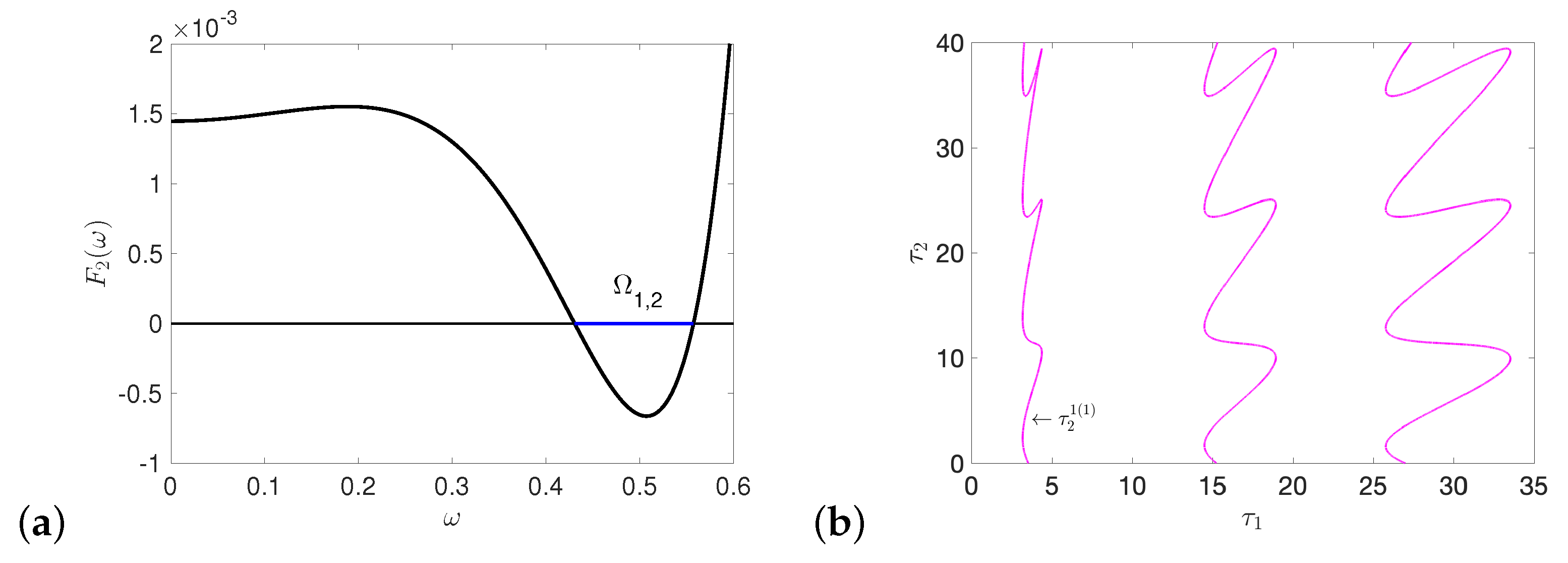
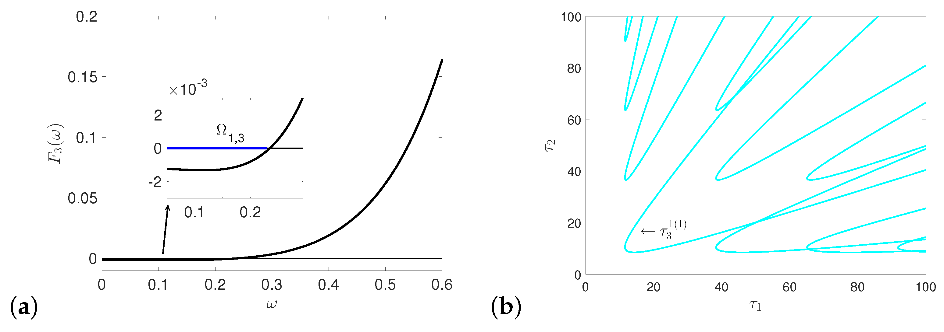
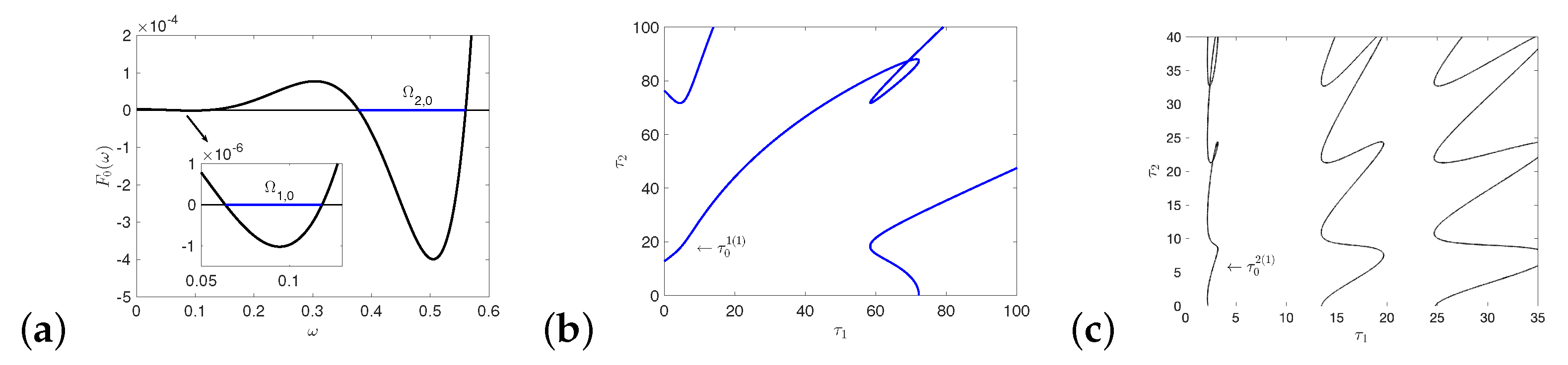
Appendix C. Stability Switching Curves
Applying the method proposed in Lin and Wang [63] to find the stability switching curves, we need to verify the assumptions (i)–(iv) in [63].
- (i)
- Finite number of characteristic roots on under the condition
- (ii)
- .
- (iii)
- are coprime polynomials.
- (iv)
- .
In fact, condition (i) follows from the work in [71]. In fact, , which is determined in (15). As we assume and for all , from Theorem 9, the constant steady state is locally asymptotically stable, and for all . Thus, condition (ii) satisfies. From the expressions of in (22), condition (iii) is obviously satisfied. From (22), we know
which means that (iv) are satisfied.
From the works in [72,73], we have the following lemma.
Lemma A1.
As the delays vary continuously in , the number of zeros (counting multiplicity) of on can change only if a zero appears on or cross the imaginary axis.
From condition (ii), is not a root of (21). Now we are in the position of seeking all the points such that has at least one root on the imaginary axis, on which the stability of equilibrium may switch. Substituting into (21),
Due to , we get that
Denote
We can easily know that there is satisfying (A2) if and only if . In fact, (A3) also includes the case .
Define
which leads to
Using the same method, we can get the corresponding results on the other delay ,
where
and the condition on is as follows:
In fact, it is easy to show that the inequality in (A3) is equivalent to the one in (A6) by squaring both sides; thus, , and we denote both of them as .
We call the set
the crossing set of characteristic equation .
Obviously, has a finite number of roots on . If , denote the roots of as
then we have If , denote the roots of as
then we have
In fact, we can confirm that when , we have , and when , we have . On two ends of , we have , and thus where . From (A4) and (A5), we can easily verify that
Denote
Thus, for the stability switching curves corresponding to , is connected to at one end , and connected to at the other end .
Denote
and
Definition A1.
Any is called a crossing point, which makes have at least one purely imaginary root with ω belongs to the crossing set . The set is called stability switching curves.
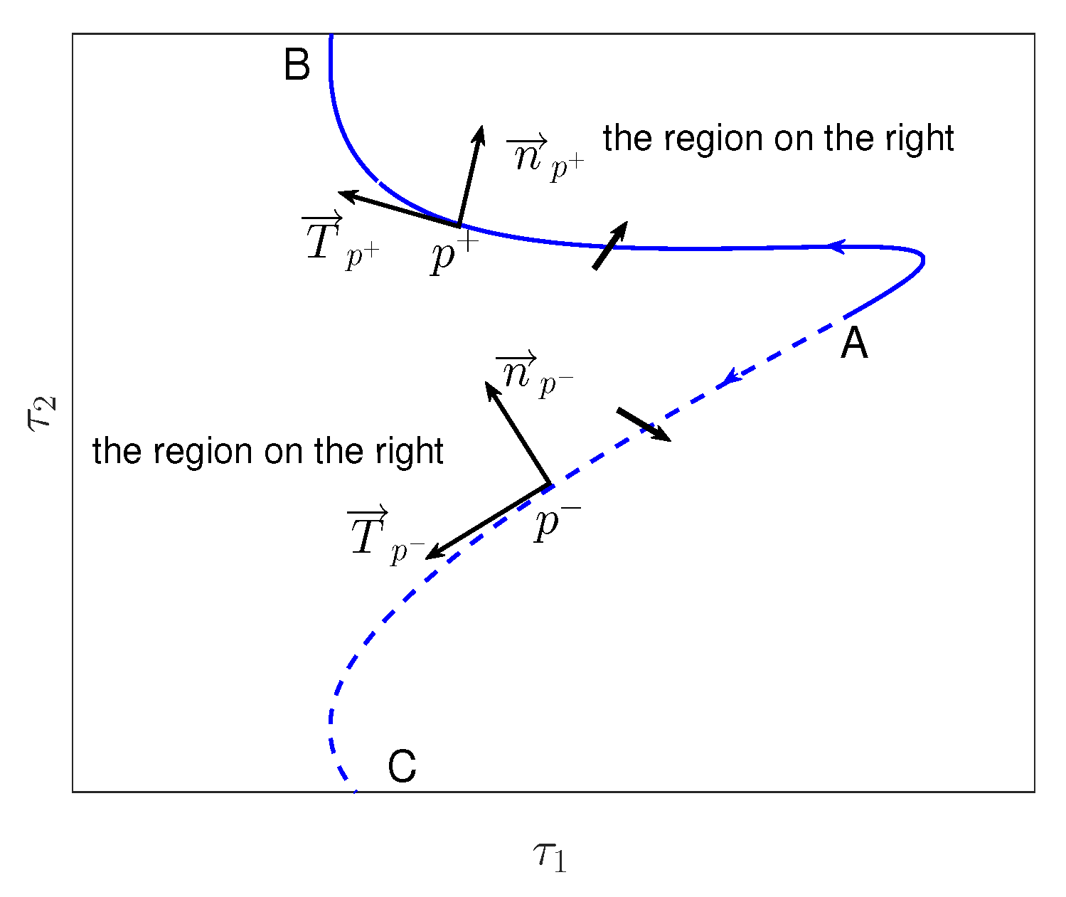
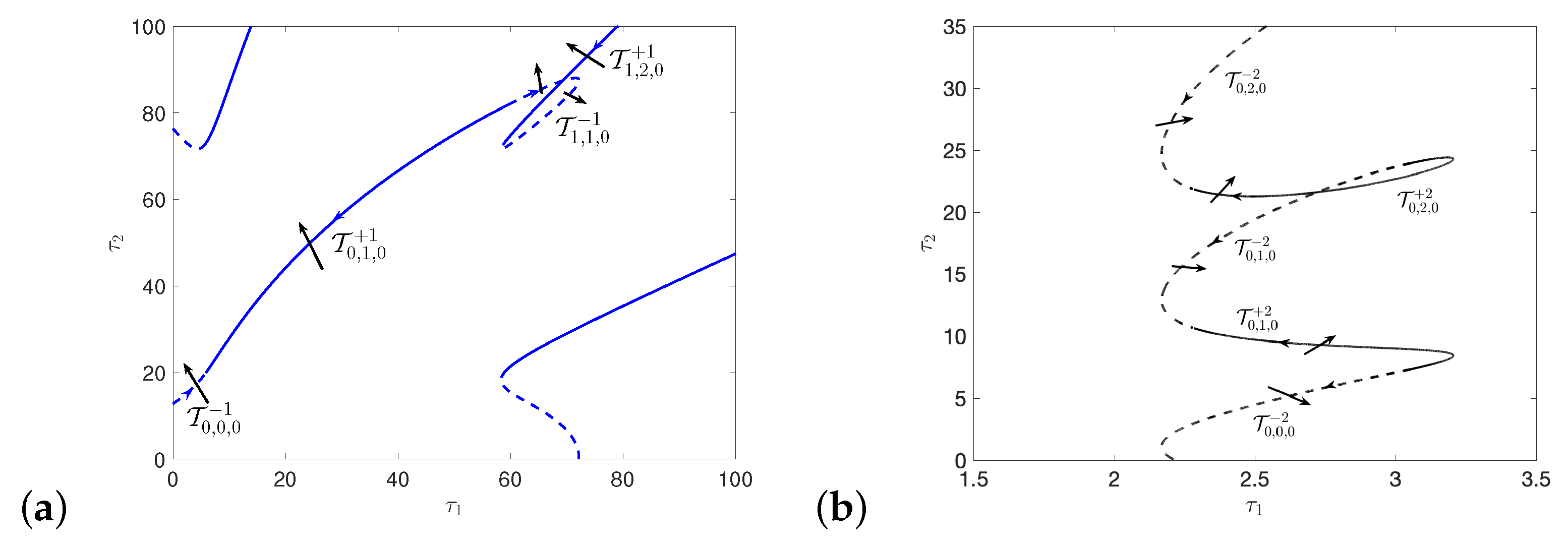
Appendix D. Crossing Directions
When varies and crosses the stability switching curves from one side to the other, the number of characteristic roots with positive real part may increase. We call it the crossing direction of stability switching curves.
In order to describe the crossing direction clearly, we need to specify the positive direction for stability switching curves . We call the direction of the curve corresponding to increasing the positive direction, i.e., from to . From the fact that is connected to at as we have mentioned in the previous subsection, the positive direction of the two curves are opposite.
To make our expression clear, we draw a schematic diagram of a part of stability switching curves corresponding to (see Figure A2). The solid curve stands for , with two ends , and . The dashed curve denotes , which is connected to at A corresponding to , with the positive direction from A to C.
Call the region on the right-hand (left-hand) side as we move in the positive directions of the curve the region on the right (left). As the tangent vector of at along the positive direction is , the normal vector of pointing to the right region is (see Figure A2). On the other hand, when a pair of complex characteristic roots cross the imaginary axis to the right half plane, moves along the direction . The inner product of these two vectors is
the sign of which can decide the crossing direction of the characteristic roots.
Figure A2.
The positive direction and crossing direction of a part of stability switching curves corresponding to .
Denote . Write (21) as
From the implicit function theorem, , can be expressed as functions of and , and if we have
with . Here, we do not consider the case that is the multiple root of , i.e., , thus we have Therefore, the sign of is decided by . We can verify that . From , we have
where denotes the interior of .
Lemma A1.
For any , we have
Thus, we can get a further conclusion which is more intuitive.
Remark A1.
The region on the right of has two more characteristic roots with positive real parts, and the region on the right of has two fewer characteristic roots with positive real parts.
Appendix E. The Figures of Stability Switching Curves
Following the steps in Appendix C and Appendix D, we can draw all the stability curves on plane and decide the crossing direction.
We can verify that and has four roots (see Figure A3a). Thus the crossing set . From (A8) and (A9), we can get the stability switching curves corresponding to which is shown in Figure A3b. To show the structure of stability switching curves and the crossing direction clearly, we take a part of curves of near the origin (i.e., in Figure A3b) as an example, and draw the figure in Figure A4a. From bottom to top, it starts with a part of , which is connected to at . is linked to at , which is again connected to at ⋯. The numerical results support the analysis result in (A7). Likewise, the stability switching curves corresponding to are shown in Figure A3c. All the stability switching curves for are given by . We also draw the leftmost curve of (marked in Figure A3c and Figure A4b). In Figure A4, the arrows on the stability switching curves represent their positive direction. From Lemma A2, we know that the regions on the right (left) of the solid (dashed) curves, which the black arrows point to, have two more characteristic roots with positive real parts.
Figure A3.
(a) The crossing set . (b) Stability switching curves . (c) Stability switching curves .
When , , and has two roots. The crossing set , which is shown in Figure A5a. We can get the stability switching curves , which are shown in Figure A5b. Thus all the stability switching curves for are given by .
Figure A5.
(a) The crossing set . (b) Stability switching curves .
When , , and has two roots, and the crossing set is , which is shown in Figure A6a, all the stability switching curves for are given by . The stability switching curves corresponding to are shown in Figure A6b.
Figure A6.
(a) The crossing set . (b) Stability switching curves .
When , , and the crossing set such that is , which is shown in Figure A7a. Moreover, the stability switching curves corresponding to are shown in Figure A7b. Thus, all the stability switching curves for are given by .
When , for any , thus there are no stability switching curves on plane for .
Figure A7.
(a) The crossing set . (b) Stability switching curves .
References
- Cosner, C.; DeAngelis, D.L.; Ault, J.S.; Olson, D.B. Effects of spatial grouping on the functional response of predators. Theor. Popul. Biol. 1999, 56, 65–75. [Google Scholar] [CrossRef] [Green Version]
- Jeschke, J.M.; Kopp, M.; Tollrian, R. Predator functional responses: Discriminating between handling and digesting prey. Ecol. Monogr. 2002, 72, 95–112. [Google Scholar] [CrossRef]
- Holling, C.S. The components of predation as revealed by a study of small-mammal predation of the European pine sawfly. Can. Entomol. 1959, 91, 293–320. [Google Scholar] [CrossRef]
- Kazarinov, N.D.; Driessche, P.V.D. A model predator-prey system with functional response. Math. Biosci. 1978, 39, 125–134. [Google Scholar] [CrossRef]
- Turchin, P. Complex Population Dynamics: A Theoretical/Empirical Synthesis; Princeton University Press: Princeton, NJ, USA, 2003. [Google Scholar]
- Song, Y.; Peng, Y.; Zhang, T. The spatially inhomogeneous Hopf bifurcation induced by memory delay in a memory-based diffusion system. J. Differ. Equ. 2021, 300, 597–624. [Google Scholar] [CrossRef]
- Schmidt, P.A.; Mech, L.D. Wolf pack size and food acquisition. Am. Nat. 1997, 150, 513–517. [Google Scholar] [CrossRef]
- Courchamp, F.; Macdonald, D.W. Crucial importance of pack size in the African wild dog Lycaon pictus. Anim. Conserv. 2001, 4, 169–174. [Google Scholar] [CrossRef] [Green Version]
- Scheel, D.; Packer, C. Group hunting behavioir of lions: A search for cooperation. Anim. Behav. 1991, 41, 697–709. [Google Scholar] [CrossRef]
- Boesch, C. Cooperative hunting in wild chimpanzees. Animal. Behav. 1994, 48, 653–667. [Google Scholar] [CrossRef] [Green Version]
- Bshary, R.; Hohner, A.; Ait-el-Djoudi, K.; Fricke, H. Interspecific communicative and coordinated hunting between groupers and giant moray eels in the Red Sea. PLoS Biol. 2006, 4, e431. [Google Scholar] [CrossRef]
- Uetz, G.W. Foraging stratigies of spiders. Trends Ecol. Evol. 1992, 7, 155–159. [Google Scholar] [CrossRef]
- Hector, D.P. Cooperative hunting and its relationship to foraging success and prey size in an avian predator. Ethology 1986, 73, 247–257. [Google Scholar] [CrossRef]
- Moffett, M.W. Foraging dynamics in the group-hunting myrmicine ant, pheidologeton diversus. J. Insect Behav. 1988, 1, 309–331. [Google Scholar] [CrossRef]
- Berec, L. Impacts of foraging facilitation among predators on predator-prey dynamics. Bull. Math. Biol. 2010, 72, 94–121. [Google Scholar] [CrossRef]
- Alves, M.T.; Hilker, F.M. Hunting cooperation and Allee effects in predators. J. Theor. Biol. 2017, 419, 13–22. [Google Scholar] [CrossRef] [PubMed]
- Jang, S.R.J.; Zhang, W.J.; Larriva, V. Cooperative hunting in a predator-prey system with Allee effects in the prey. Nat. Resour. Model. 2018, 31, e12194. [Google Scholar] [CrossRef]
- Pal, S.; Pal, N.; Samanta, S.; Chattopadhyay, J. Effect of hunting cooperation and fear in a predator-prey model. Ecol. Complex. 2019, 39, 100770. [Google Scholar] [CrossRef]
- Sen, D.; Ghorai, S.; Banerjee, S.M. Allee effect in prey versus hunting cooperation on predator-enhancement of stable coexistence. Int. J. Bifurc. Chaos 2019, 29, 1950081. [Google Scholar] [CrossRef]
- Yan, S.; Jia, D.; Zhang, T.; Yuan, S. Pattern dynamics in a diffusive predator-prey model with hunting cooperations. Chaos Solitons Fract. 2020, 130, 109428. [Google Scholar] [CrossRef]
- Wu, D.Y.; Zhao, M. Qualitative analysis for a diffusive predator-prey model with hunting cooperative. Phys. A 2019, 515, 299–309. [Google Scholar] [CrossRef]
- Song, D.X.; Li, C.; Song, Y.L. Stability and cross-diffusion-driven instability in a diffusive predator-prey system with hunting cooperation functional response. Nonlinear Anal. RWA 2020, 54, 103106. [Google Scholar] [CrossRef]
- Pal, S.; Pal, N.; Chattopadhyay, J. Hunting cooperation in a discrete-time predator-prey system. Int. J. Bifurc. Chaos 2018, 28, 1850083. [Google Scholar] [CrossRef]
- Pati, N.C.; Layek, G.C.; Pal, N. Bifurcations and organized structures in a predator-prey model with hunting cooperation. Chaos Soliton Fract. 2020, 140, 110184. [Google Scholar] [CrossRef]
- Chou, Y.H.; Chow, Y.S.; Hu, X.C.; Jang, S.R.J. A Ricker-type predator-prey system with hunting cooperation in discrete time. Math. Comput. Simulat. 2021, 190, 570–586. [Google Scholar] [CrossRef]
- Chow, Y.S.; Jang, S.R.J.; Wang, H.M. Cooperative hunting in a discrete predator–prey system. Int. J. Biomath. 2000, 13, 2050063. [Google Scholar] [CrossRef]
- Allee, W.C. The Social Life of Animals; William Heinemann: London, UK, 1938. [Google Scholar]
- Courchamp, F.; Berec, L.; Gascoigne, J. Allee Effects in Ecology and Conservation; Oxford University Press: Oxford, UK, 2008. [Google Scholar]
- Wang, J.F.; Shi, J.P.; Wei, J.J. Predator-prey system with strong Allee effect in prey. J. Math. Biol. 2010, 62, 291–331. [Google Scholar] [CrossRef] [PubMed]
- Conway, E.D.; Smoller, J.A. Global analysis of a system of predator-prey equations. SIAM J. Appl. Math. 1986, 46, 630–642. [Google Scholar] [CrossRef]
- Song, Y.; Jiang, H.; Yuan, Y. Turing-Hopf bifurcation in the reaction-diffusion system with delay and application to a diffusive predator-prey model. J. Appl. Anal. Comput. 2019, 9, 1132–1164. [Google Scholar] [CrossRef]
- Xu, X.; Wei, J. Turing-Hopf bifurcation of a class of modified Leslie-Gower model with diffusion. Disc. Contin. Dyn. Sys. B 2018, 23, 765–783. [Google Scholar] [CrossRef] [Green Version]
- An, Q.; Jiang, W. Spatiotemporal attractors generated by the Turing-Hopf bifurcation in a time-delayed reaction-diffusion system. Disc. Contin. Dyn. Syst. B 2019, 24, 487–510. [Google Scholar] [CrossRef] [Green Version]
- Guo, G.; Liu, L.; Li, B.; Li, J. Qualitative analysis on positive steady-state solutions for an autocatalysis model with high order. Nonlinear Anal. RWA 2018, 41, 665–691. [Google Scholar] [CrossRef]
- Kuang, Y. Delay Differential Equations: With Applications in Population Dynamics; Academic Press: Boston, MA, USA, 1993. [Google Scholar]
- Gopalsamy, K. Stability and Oscillations in Delay Differential Equations of Population Dynamics; Springer: Dordrecht, The Netherlands, 1992. [Google Scholar]
- Martin, A.; Ruan, S.G. Predator-prey models with delay and prey harvesting. J. Math. Biol. 2001, 43, 247–267. [Google Scholar] [CrossRef]
- Xia, J.; Liu, Z. H; Yuan, R. The effects of harvesting and time delay on predator-prey systems with Holling type II functional response. SIAM J. Appl. Math. 2009, 70, 1178–1200. [Google Scholar] [CrossRef] [Green Version]
- Shi, J.P.; Wang, C.C.; Wang, H. Diffusive spatial movement with memory and maturation delays. Nonlinearity 2019, 32, 3188–3208. [Google Scholar] [CrossRef] [Green Version]
- Wright, E. A functional equation in the heuristic theory of primes. Math. Gaze. 1961, 45, 15–16. [Google Scholar] [CrossRef]
- May, R.M. Time delay versus stability in population models with two and three trophic levels. Ecology 1973, 54, 315–325. [Google Scholar] [CrossRef]
- Xu, C.; Tang, X.; Liao, M.; He, X. Bifurcation analysis in a delayed Lokta-Volterra predator-prey model with two delays. Nonlinear Dyn. 2011, 66, 169–183. [Google Scholar] [CrossRef]
- Yan, X.P.; Zhang, C.H. Hopf bifurcation in a delayed Lotka-Volterra predator-prey system. Nonlinear Anal. RWA 2008, 9, 114–127. [Google Scholar] [CrossRef]
- Jankovic, M.; Petrovskii, S. Are time delay always destabilizing? Revisiting the role of time delays and the Allee effect. Theor. Ecol. 2014, 7, 335–349. [Google Scholar] [CrossRef] [Green Version]
- Cooke, K.L.; Driessche, P.V.D. Analysis of an SEIRS epidemic model with two delays. J. Math. Biol. 1996, 35, 240–260. [Google Scholar] [CrossRef]
- Freedman, H.I.; Rao, V.S.H. Stability criteria for a system involving two time delays. SIAM J. Appl. Math. 1986, 46, 552–560. [Google Scholar] [CrossRef]
- Wei, J. J, Ruan, S.G. Stability and bifurcation in a neural network model with two delays. Physica D 1999, 130, 255–272. [Google Scholar] [CrossRef]
- Xu, J.; Chung, K.W.; Chan, C.L. An efficient method for studying weak resonant double Hopf bifurcation in nonlinear systems with delayed feedbacks. SIAM J. Appl. Dyn. Syst. 2007, 6, 29–60. [Google Scholar] [CrossRef] [Green Version]
- Du, Y.F.; Niu, B.; Wei, J.J. Two delays induce Hopf bifurcation and double Hopf bifurcation in a diffusive Leslie-Gower predator-prey system. Chaos 2019, 29, 013101. [Google Scholar] [CrossRef] [PubMed]
- Huang, C.X.; Yang, Z.C.; Yi, T.S. On the basins of attraction for a class of delay differential equations with non-monotone bistable nonlinearities. J. Differ. Equ. 2014, 256, 2101–2114. [Google Scholar] [CrossRef]
- Huang, C.X.; Zhao, X.; Cao, J.D.; Alsaadi, F.E. Global dynamics of neoclassical growth model with multiple pairs of variable delays. Nonlinearity 2020, 33, 6819–6834. [Google Scholar] [CrossRef]
- Yu, P.; Yuan, Y.; Xu, J. Study of double Hopf bifurcation and chaos for oscillator with time delay feedback. Commun. Nonlinear Sci. Numer. Simul. 2002, 7, 69–91. [Google Scholar] [CrossRef]
- Du, Y.F.; Niu, B.; Guo, Y.X.; Wei, J.J. Double Hopf bifurcation in delayed reaction-diffusion systems. J. Dynam. Differ. Equ. 2020, 32, 313–358. [Google Scholar] [CrossRef] [Green Version]
- Ma, S.; Lu, Q.; Feng, Z. Double Hopf bifurcation for van der Pol-Duffing oscillator with parametric delay feedback control. J. Math. Anal. Appl. 2008, 338, 993–1007. [Google Scholar] [CrossRef] [Green Version]
- Campell, S.A.; Bélair, J.; Ohira, T.; Milton, J. Limit cycles, tori, and complex dynamics in a second-order differential equations with delayed negative feedback. J. Dynam. Differ. Equ. 1995, 7, 213–236. [Google Scholar] [CrossRef]
- Acosta-Humánez1, P.B.; Yagasaki, K. Nonintegrability of the unfoldings of codimension-two bifurcations. Nonlinearity 2020, 33, 1366–1387. [Google Scholar] [CrossRef] [Green Version]
- Ge, J.H.; Xu, J. An analytical method for studying double Hopf bifurcations induced by two delays in nonlinear differential systems. Sci. China-Technol. Sci. 2019, 63, 597–602. [Google Scholar] [CrossRef]
- Rosenzweig, M.L.; MacArthur, R. Graphical representation and stability conditions of predator-prey interactions. Am. Nat. 1963, 97, 209–223. [Google Scholar] [CrossRef]
- Rosenzweig, M.L. Why the prey curve has a hump? Am. Nat. 1969, 103, 81–87. [Google Scholar] [CrossRef]
- Hsu, S.B. On global stability of a predator-prey system. Math. Biosci. 1978, 39, 1–10. [Google Scholar] [CrossRef] [Green Version]
- Wiggins, S. Introduction to Applied Nonlinear Dynamical Systems and Chaos; Springer: New York, NY, USA, 1990. [Google Scholar]
- Guckenheimer, J.; Holmes, P. Nonlinear Oscillations, Dynamical Systems, and Bifurcations of Vector Fields; Springer: New York, NY, USA, 1983. [Google Scholar]
- Lin, X.; Wang, H. Stability analysis of delay differential equations with two discrete delays. Can. Appl. Math. Q. 2012, 20, 519–533. [Google Scholar]
- Wu, J. Theory and Applications of Partial Functional-Differential Equations; Springer: New York, NY, USA, 1996. [Google Scholar]
- Faria, T. Normal forms and Hopf bifurcation for partial differential equations with delays. Trans. Am. Math. Soc. 2000, 352, 2217–2238. [Google Scholar] [CrossRef]
- Polking, J.A.; Arnold, D. Ordinary Differential Equations Using MATLAB; Prentice-Hall: Englewood Cliffs, NJ, USA, 2003. [Google Scholar]
- Dhooge, A.; Govaerts, W.; Kuznetsov, Y.A. MATCONT: A MATLAB package for numerical bifurcation analysis of ODEs. ACM Trans. Math. Softw. 2003, 29, 141–164. [Google Scholar] [CrossRef]
- Alexander, J.C.; Yorke, J.A. Global bifurcations of periodic orbits. Am. J. Math. 1978, 100, 263–292. [Google Scholar] [CrossRef]
- Chow, S.N.; Mallet-Paret, J. The Fuller index and global Hopf bifurcation. J. Differ. Equ. 1978, 29, 66–85. [Google Scholar] [CrossRef] [Green Version]
- Wu, J. Symmetric functional-differential equations and neural networks with memory. Trans. Am. Math. Soc. 1998, 350, 4799–4838. [Google Scholar] [CrossRef]
- Hale, J. Theory of Functional Differential Equations; Springer: New York, NY, USA, 1977. [Google Scholar]
- Cooke, K.L.; Grossman, Z. Discrete delay, distributed delay and stability switches. J. Math. Anal. Appl. 1982, 86, 592–627. [Google Scholar] [CrossRef] [Green Version]
- Ruan, S.G.; Wei, J.J. On the zeros of transcendental functions with applications to stability of delay differential equations with two delays. Dyn. Contin. Discret. Impuls. Syst. Ser. A Math. Anal. 2003, 10, 863–874. [Google Scholar]
Publisher’s Note: MDPI stays neutral with regard to jurisdictional claims in published maps and institutional affiliations. |
© 2021 by the authors. Licensee MDPI, Basel, Switzerland. This article is an open access article distributed under the terms and conditions of the Creative Commons Attribution (CC BY) license (https://creativecommons.org/licenses/by/4.0/).