Abstract
The hub location problem (HLP) basically consists of selecting nodes from a network to act as hubs to be used for flow traffic directioning, i.e., flow collection from some origin nodes, probably transfer it to other hubs, and distributing it to destination nodes. A potential expansion on the hub building and capacitated modules increasing along a time horizon is also considered. So, uncertainty is inherent to the problem. Two types of time scaling are dealt with; specifically, a long one (viz., semesters, years), where the strategic decisions are made, and another whose timing is much shorter for the operational decisions. Thus, two types of uncertain parameters are also considered; namely, strategic and operational ones. This work focuses on the development of a stochastic mixed integer linear optimization modeling framework and a matheuristic approach for solving the multistage multiscale allocation hub location network expansion planning problem under uncertainty. Given the intrinsic difficulty of the problem and the huge dimensions of the instances (due to the network size of realistic instances as well as the cardinality of the strategic scenario tree and operational ones), it is unrealistic to seek an optimal solution. A matheuristic algorithm, so-called SFR3, is introduced, which stands for scenario variables fixing and iteratively randomizing the relaxation reduction of the constraints and variables’ integrality. It obtains a (hopefully, good) feasible solution in reasonable time and a lower bound of the optimal solution value to assess the solution quality. The performance of the overall approach is computationally assessed by using stochastic-based perturbed well-known CAB data.
1. Introduction and Motivation
The hub location problem (HLP) basically consists of selecting nodes from a network to be used for flow traffic directioning, i.e., flow collection from some origin nodes, probably transfer it to other hubs, and distributing it to destination nodes. Examples can be found in product distribution, telecommunications, land and air transportation, etc. As a matter of fact, an HLP can be considered in any flow supplying problem where, instead of directly delivering from origin to destination, there is an opportunity (due to capacity limitations and economic reasons, among others) for performing hub transfer to delivering flow from different pairs of origin-destination. See, for instance, the multiperiod deterministic problem presented in [1], where a case study of humanitarian aid distribution in Lebanon is considered. The hub building and operational overall cost are the functions to be minimized in most of the problems. Real-life multiperiod problems are frequently encountered in industry where the hub capacity needs to be expanded and/or additional hubs are required to satisfy the flow demand from one node to another; see [2,3]. The stochasticity on the main parameters is inherent to multiperiod problems; see [4,5]. The hubs can be capacitated or uncapacitated, and the problem can be deterministic or stochastic, and static (i.e., single period) or dynamic along a time horizon. Let the dynamic HLP be named as a multiperiod one for the deterministic and two-stage multiperiod settings, and a multistage one for the other stochastic settings, where the uncertainty is either a stage-dependent, stagewise one, or even both types in a multiscale setting. The NP-hardness of HLP is proven in [6], even for the single-allocation uncapacitated p-hub location deterministic version, where p hubs must be located and non-hub nodes are allocated to the hub ones. This type of problems is a particular case of the one that is addressed in this work.
There is broad literature on the subject, see [2,7,8]; recent reviews and some perspectives on modelling are presented in [9,10]. However, the literature is scarce on the inherent stochasticity of HLP, to the best of our knowledge, there are no works on multistage stochastic HLP.
This work deals with the multistage multiscale stochastic capacitated HLP with network expansion along a time horizon. The uncertainty of the strategic parameters is assumed to be stagewise-dependent and the one of the operational parameters is assumed to be stage-dependent. So, a multiscale setting is addressed, as it frequently happens in reality. Given the network size of realistic instances as well as the cardinality of the strategic scenario tree and operational ones, it is a challenge to deal with the intrinsic difficulty of the problem and the huge dimensions of the instances. It is therefore unrealistic to seek an optimal solution for the deterministic equivalent model (DEM) of the tight stochastic mixed integer linear optimization one (traditionally, named MILP) that is presented. In contrast, a matheuristic algorithm, so-called SFR3, is introduced for achieving (hopefully, good) feasible solutions jointly, with a lower bound of the optimal solution value to assess the solution quality.
The rest of the work is organized as follows: Section 2 presents the problem’s assumptions. For completeness purposes and setting some notation to be used throughout the work, Section 2.1 also recalls the main concepts of the strategic multistage scenario tree with embedded operational two-stage ones. Section 3 is devoted to a literature review on the subject, and outlines the main contributions of the work. Section 4 presents the model for MS-Hub-NEP. Section 5 introduces the matheuristic algorithm SFR3. Section 6 reports the main results of the computational experiment. Section 7 draws the main conclusions, and its Section 7.1 outlines the perspectives of model MS-Hub-NEP and maheuristic SFR3, as well as a future research agenda. An example is presented in Appendix A to illustrate the main decisions to be made in MS-Hub-NEP and the role of the scenario trees. Appendix B reports the results of the computational comparison between SFR3 strategies.
2. MS-Hub-NEP Problem Description
The section has two parts; first, the problem is presented jointly with the related sets. Secondly, Section 2.1 recalls the main elements of the strategic multistage scenario tree and related operational two-stage ones, also introducing the location-allocation elements for the strategic and operational scenarios.
The features of the Multistage Stochastic-Hub Network Expansion Planning problem (MS-Hub-NEP) are presented. The time horizon is finite and divided into time units, so-called stages. All nodes in the network (even the hubs) can have flow outbound, inbound or both. Without loss of generality, the set of potential hub locations is assumed to be a subset of the nodes in the network. A hub can have outbound and inbound flows. Hub building (a strategic decision) is performed at the beginning of the stages. The hubs are capacitated, so, the number of initial capacity modules should be decided, in the case of building. An expansion on the number of modules (another strategic decision) could be decided at later stages. A maximum number of capacity modules is imposed for each hub; all modules have the same capacity (i.e., they are assumed to be technically identical). The number of available hubs at the stages is bounded. The flow from origin node, say i, destined to another one, say j, can be transported (an operational decision) by using the so-called non-stop service mode or, alternatively, the transportation can be done through the hub network. The unit transportation cost is a function of the distance between the nodes. The assumption of two hubs to be used, at most, to transfer a given origin-destination flow through the hub network, is not always realistic. However, it is one of the main assumptions of the work and, even in this case, the problem is still very difficult to solve. By using the notation k and l for the hubs involved, the route can be , or . If the non-stop service mode between any two network nodes is decided, then one of those nodes, at most, could be hub available. The allocation of nodes to hubs can be changed from a stage to another. In stochastic optimization parlance, it means that the allocation can be changed from a strategic node to each of its immediate successors. The number of origin nodes to allocate to any hub could be bounded.
As an illustrative example, let us assume that the strategic decisions have already been made, based on the hub building and capacity module strategic costs, the transportation costs, and the flow demand. So, let hubs 1 and 3 be available at, say, stage 1 with a given capacity; see Figure 1. The figure also shows the operational decisions that have been assumed for a given operational scenario. Those decisions are related to transporting the flow demand from origin i to destination j, perhaps through hubs k and l. That is, it shows the routes , or , for the flow of each network node pair . Suppose that the operational decisions are made as follows: Flow demand in the non-stop service mode, , and ; , collection at hub 3 of flow demand from node 8; , collection at hub 3 of flow demand from node 8 with destination node 4; , collection at hub 3 of flow demand from node 8 that is transferred to hub 1 with destination node 5; and , collection at hub 1 of flow demand from node 6 with destination nodes 4 and 5, resp.; and , collection at hub 1 of flow demand from node 2 that is transferred to hub 3 with destination node 9. Observe that hub 3 is inbound under the assumed operational scenario, being the destination of a portion of the flow demand from origin node 8. Note that the hub edge is used in both senses for hubs 1 and 3 since, on one hand, it transfers the flow demand from node 2 to node 9 and, on the other hand, it transfers it from node 8 to node 5.
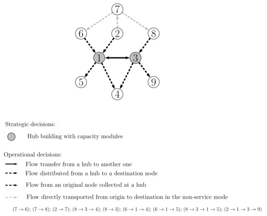
Figure 1.
Origin and destination network nodes and hubs representation. Operational decisions.
Sets for the Hub Network
Let the following notation, where capital letters represent data, calligraphic symbols do it for sets, and are indices.
- , network nodes.
- , candidate hubs.
- , pairs of origin node i and destination node j, each one denoted as . Note that hub k can also be any of those nodes, for .
- , ’distance’ between nodes i and j, for .Recall that the edge types in the hub network are as follows: origin node to hub, hub to hub, and hub to destination node.
- , maximum ’distance’ that is allowed for any hub edge in the network. It is worth pointing out that link is not allowed for .
For the purpose of reducing the number of variables and constraints related to the operational scenarios in the model below, the strengthening sets are as follows:
- , hub pair set for flow transfer in the directions from k to l and l to k) in case of their availability.
- , hub pair set for flow transfer from origin node i in the direction k to l, for .
- , hub pair set for flow transfer from origin node i in the direction l to k, for .
- , hub set for flow collecting from origin node i, where it is directly distributed to destination node j, for , such that . Any of the hubs i and j can be in (but not both), such that if hub i is outbound and if hub j is inbound.
- , hub set for flow collecting from origin node i, for , such that either the collected flow at a hub is transferred to another, or it is directly distributed to the appropriate nodes. Note: Hub i can be in .
Remark 1.
for .
2.1. Strategic Multistage Operational Two-Stage Stochastic Trees
The notation of multistage and two-stage scenario trees to be used in this work is recalled from [11].
Strategic Multistage Stochastic Tree
Let a strategic scenario be the realization of the uncertain strategic parameters (i.e., hub-related building and capacity module installation costs) along the time horizon. A strategic node for a given stage has one-to-one correspondence with the group of strategic scenarios that have the same realization of the uncertain parameters up to the stage. This information structure can be visualized as the tree depicted in Figure 2, where each root-to-leaf path represents a specific scenario and, then, it corresponds to a realization of the whole set of the uncertain parameters. Let us point out that it is beyond the scope of this work to present a methodology for multistage scenario tree generation and reduction; see e.g., [12,13] and references therein.
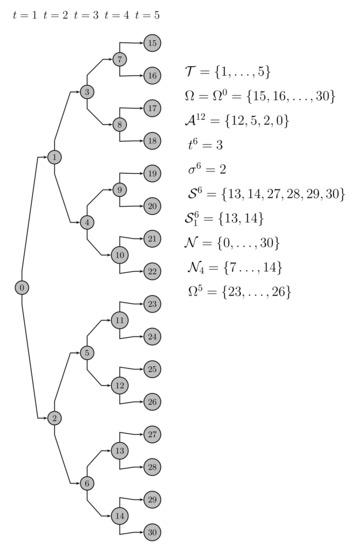
Figure 2.
Strategic multistage scenario tree.
The notation for the lexicographically ordered sets in the strategic tree is as follows:
- , stages, and .
- , nodes in the scenario tree, such that , and .
- , nodes in stage t, where , for . Note: By construction, =1.
- , scenarios. Each one is included by the nodes in the Hamiltonian path from the root node 0 to a node, say, in the last stage, through the ones in set ; so, .Note: For convenience, a scenario has traditionally been denoted by its last node in the path.
- , scenarios having one-to-one correspondence with node n.
- , node n and its ancestors, for . Note that is only included by node 0, where .
- , successors nodes of node n, for . Note: , for .
- , immediate successors of node n, for .
Let the following other elements in the strategic scenario tree:
- , weight factor representing the likelihood that is associated with node n, for . Note: , where gives the modeler-driven likelihood associated with scenario , such that .
- , stage to which node n belongs to, so, .
- , immediate ancestor node of node n, for . Note: It is assumed that is not necessarily null, since it is allowed that the hub network already exists before the beginning of the time horizon; so, in that case, the aim of the proposal is the hub expansion along the time horizon.
As an illustration, let the instance with stages and a scenario tree where the number of strategic immediate successor nodes of node n is for . So, the cardinality of the strategic scenario tree is nodes, see Figure 2.
Operational Two-Stage Trees Rooted at Strategic Nodes
The operational uncertainty is represented in a finite set of stage-dependent scenarios. It is structured in a two-stage tree rooted at any strategic node in set . So, the operational realizations (i.e., scenarios) are visualized in the nodes of the second stage. Let us introduce the following additional notation:
- , set of operational scenarios in stage t, for .
- , weight factor or probability of operational scenario , for , such that , for .
So, it is assumed that the operational uncertainty in MS-Hub-NEP (e.g., flow demand) is independent of the strategic one.
Following on from the illustration of the strategic tree dimensions considered above, let us assume that there are operational scenarios in the two-stage tree rooted at any strategic node that belongs to stage t in the scenario tree with strategic ones. So, in total, there are 124 uncertain operational situations to be dealt with, being partitioned into 31 groups. It means that there are 124 hub operational (static deterministic) interconnected submodels, see next. Thus, the submodels related to the nodes in set , for , have the same initial infrastructure topology (i.e., initial set of available hubs). Figure 3 depicts the illustrative strategic and operational trees, where, e.g., , for any strategic node in set . For it results that there are 248 hub operational submodels. See, in Section 6, a broad computational experience.
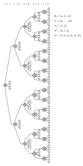
Figure 3.
Strategic multistage scenario tree with operational two-stage scenario trees.
Remark 2.
For the unlikely case where the strategic nodes in MS-Hub-NEP are also stagewise-dependent on the operational ones then, instead of the tree depicted in Figure 3, the full combination of strategic and operational scenarios results in a gigantic multistage scenario tree. For ease of presenting, let us assume the frequent case where the multistage scenario tree is symmetric. Additionally, let us consider the two following alternative decision making frameworks at stage t. The first one is a two-step framework, where the strategic decisions are carried out at step 1 by considering all the potential operational scenarios that can occur at step 2 of the stage as above. In the second framework, it is assumed that the strategic decisions are delayed until the operational uncertainty is unveiled and, then, both types of decisions are made simultaneously, so, only one step is considered. Thus, let the new 0–1 parameter take the value 1 for the first framework in stage t, and otherwise, 0. So, for , there are two types of nodes in each stage: strategic and operational. The operational nodes are the leaf ones in the stage. Let and, for this purpose, denote the leaf node subset and the node set in stage t, resp, for , being expressed as , , and and , where gives the number of strategic nodes in stage t for the immediate ancestor, . As an example, for , and , the dimensions of the scenario tree are = 23,405 nodes and = 16,384 scenarios for , and 629,145 nodes and 524,288 scenarios for . Observe that each scenario has a one-to-one correspondence with a hub strategic-operational multiperiod deterministic submodel. So, it is useful to consider the proposed approximation type in order to have an affordable structure.
Location-Allocation Parameters for Strategic and Operational Scenarios
- , maximum number of hubs that can be available at any strategic node n that belongs to stage t, for .
- , maximum number of origin nodes that can be allocated to a hub (i.e., whose flow can be collected) in any strategic node that belongs to set , for .
- ,,maximum number of capacity modules that can be available at hub k, for .
- K, flow capacity of a module in any hub. Note: The modules are assumed to be identical.
- Costs Related to Hub k in Strategic Node n, for
- , hub building cost.
- , installation cost of an initial capacity module at the hub.
- , installation cost of an additional capacity module at the hub.
- , maintenance cost of a capacity module at hub k in stage t, for . Note: It is the expected cost in the operational scenarios in stage t that also depends on the hub location.
Costs Related to Operational Scenario π in Stage t, for
- , flow allocation setup cost of origin node i to hub k, for .
- , flow transfer setup cost through hub edge , for .
- , flow transportation setup cost from origin node i to destination node j in case the non-stop service mode is chosen, for .
- , unit cost of flow (a) collection from origin node i at hub j, for , (b) transfer through hub edge , for , and (c) distribution from hub i to destination node j, for . Note: (resp., ) is zero for hub outbound (resp., inbound) flow, where (resp., ).
Note: All costs should be computed by considering the net present value.
Flow from Origin to Destination under Operational Scenario π in Stage t, for
- , flow demand from origin node i to destination node j under scenario , for .
- , overall flow originated in node i under scenario , computed as , for .
Problem Decisions
- At the strategic nodes of the multistage scenario tree: location of the new hubs and number of initial capacity modules to be installed as well as the additional ones to be installed in the successor strategic nodes, if any.
- Under the operational scenarios in the two-stage trees, being rooted at the strategic nodes: flow from origin nodes to be collected in the hubs, flow transferred from one hub to another one, if any, flow distributed from the hubs to the destination nodes, and flow directly transported from origin to destination in the non-stop service mode.
The objective is to minimize the expected hub building cost, the expected cost of initial and additional capacity modules installation, and the expected cost of hub maintenance, operation and routing flow along the time horizon.
3. HLP Literature Review
Let us look at the following HLP categories:
3.1. Static Deterministic Hub Location
Most of the works in the literature on hub location and operation (up to 2016, at least) are usually related to a single period. Its key elements are assumed to be known with certainty, such the origin-destination flow demand, the hub availability, and the strategic and operational costs, among others. The hubs are frequently assumed to be uncapacitated ones, and different types of MILP models are introduced, as well as a few nonlinear ones. See the seminal works [14,15,16], and a survey of HLPs up to the early 1990s in [17]. An integer model for the Euclidean uncapacitated HLP is presented in [18], jointly with an algorithm to consider the set of valid inequalities that, in a Lagrangean relaxation framework, seem to be tighter to reduce the branch-and-bound (B&B) burden. Several MILP models are presented in [19] for the capacitated HLP, and tight valid inequalities are identified in a B&B algorithm. A survey of HLPs is presented in [20], where some real-world applications, models and decomposition algorithms for problem solving are reviewed by considering works in the literature from 2013 to 2016. A further comprehensive review is presented in [21] for the classical HLP.
The design of intermodal HLPs is reviewed in [10], where most of the 100 works that are considered were published between 2014 and 2020. Most of those works are static deterministic MILP models, very few are multiperiod ones, and the literature dealing with uncertainty is very scarce, mainly devoted to dealing with disruptive events at the hubs and the links. A capacitated intermodal transportation hub network model is presented in [22], where spoke-to-hub and hub-to-spoke transportation is allowed. A real-life problem of a Turkish public institution is considered for validating the proposed approach for problem solving. A MILP model for a capacitated multimodal, multicommodity HLP is presented in [23], where a non-stop service mode (i.e., a direct transportation from origin to destination) is considered as the hub network alternative.
A profit maximization is presented in [24] for a multicommodity multiple node allocation to hubs in a singular HLP, where the design (here, so-called strategic) decisions are as follows: nodes where hubs are located (satisfying the triangular inequality); node selection as origin or destination of commodity, at least, to serve; and hub edges selection to be used for transferring a commodity, at least. All of them are represented by binary variables. Operational decisions for the commodities, in case of being serviced, are those related to traffic through the network. All of them are represented by binary variables and, since, the problem is uncapacitated, the integrality is relaxed, due to the fact that an optimal solution guarantees that feature. A sophisticated Lagrangan relaxation is considered, where the optimality of the solution is guaranteed.
Two formulations are presented in [25] for the uncapacitated HLP, where the flow transfer between more than two hubs is allowed. Mixed integer-based approaches for dealing with discrete multiple location-allocation hub-centroid problems are presented in [26] and references therein. In that work, two non-cooperative agents, the leader and the follower, are considered for locating hubs to compete for the same market in a static setting.
A mixed integer nonlinear optimization (traditionally, named MINLP) model for a single period single allocation CHL problem is presented in [27], where the capacity is represented by a set of exclusive modules of different size, and two hubs are allowed, at most for flow transfers. The flow congestion in the hubs, see [28], is key in the approach, being introduced with non-linearities in the objective function. It is partially linearized by converting it into alternate partial linearizations, so that several mixed integer second order conic program-based reformulations are also proposed.
The HLP-Ordered Median Tree problem (HLP-OMTP) is presented in [29] in its single-allocation unconstrained version, where each network node is only allocated to one hub, and a given number of hubs should be located. The objective function to minimize is the weighted average cost of the ordered flow collection and distribution, as well as the hub edges flow. Several Minimum Spanning Tree and OMTP-based binary linear optimization models are introduced. A unified approach of the single-allocation OMTP is presented in [30], where a MILP model is considered.
3.2. Multiperiod Deterministic Hub Location
Multiperiod models are very scarce given the problem’s difficulty; however, as noted in [31], ‘ignoring the multiperiod nature of the problem might considerable formulations affect costs’. A good review of multiperiod hub network expansion planning (NEP) modeling and algorithmic approaches is presented in [2]. Among the very few works in the literature dealing with the multiperiod NEP problem, A MILP model for the uncapacitated hub NEP (MUNEP) is presented in [32]. A B&B approach is proposed for problem solving, where a Lagrangean relaxation is considered for decomposing the model into smaller submodels, by exploiting the NEP structure, and some reduction procedures are also presented. Another MILP model is presented in [3] for MUNEP, where the leasing of the hubs is performed along the time horizon, as well as the termination of the existing contracts. Two approaches for problem solving are proposed; namely, an extension of the Benders algorithm and a metaheuristic one. The latter is based on neighborhood structures, so that the algorithm moves from one feasible solution (given by a set of hubs and hub edges) to another one within the neighborhood of the former.
A MILP model is presented in [31] for the multiperiod capacitated NEP, where single and multiple allocation variants are considered, and tight valid inequalities are generated and appended to the model. Some MILPs for multiperiod multimodal NEP with hub and hub edge capacity degradations due to disruptive events are presented in [33,34]. A problem with serial demands is presented in [1], where a set of valid inequalities are identified and appended to the original MILP model. A Benders cut algorithm is introduced, and the approach is validated by considering a case study of humanitarian aid distribution in Lebanon.
3.3. Static Stochastic Hub Location
Most of the works in the literature on static stochastic location are usually related to network infrastructure stochastic disruptions, due to natural disasters and terrorist attacks. See in [35] a comprehensive review on the subject. Additionally, a MINLP model presented for the single-allocation capacitated HLP with stochastic complete and partial hub disruptions and stochastic partial hub edges (i.e., hub network links). A bi-objective framework is considered for the minimization of the total cost and the maximum transportation time, in order to get lower bounds for the Pareto-frontier. By appropriate approximations, the nonlinear chance constraints are converted into linear ones, and then a MILP model is considered. Near optimal Pareto solutions are obtained by two metaheuristics, namely, a genetic algorithm and a variable neighborhood search-based algorithm.
3.4. Two-Stage Stochastic Hub Location
The key parameters in HLP are frequently uncertain in the decision making process in real-life problems; however, the literature on stochastic hub NEP is very scarce. The realization of the uncertain parameters in mathematical optimization can usually be structured in a representative finite set of scenarios along the periods in a time horizon. Traditionally, special attention has been paid to optimize the DEM of the stochastic model by, in this case, minimizing the expected hub network location and operation in the scenarios. Obviously, that optimization is subject to the satisfaction of the problem constraints for each of the realizations (i.e., scenarios) that have been considered for representing the uncertainty of the main parameters. Thereafter, it will be referred to as the risk neutral (RN) problem. The parameters’ uncertainty in HLP has been studied since the 1960s, see, recently, [5,36]. Most of the works in the literature deal with two-stage static stochastic models, and related algorithms for problem solving.
The capacitated/uncapacitated hub location decisions (referred to in this work as strategic ones) under uncertainty are considered as first stage variables in the models. No subordination is made to a single scenario, but all of them are considered as a whole for decision making. On the other hand, the (referred to in this work as operational) decisions on allocation of origin-destination flow demands from one hub to another are considered as second stage variables in the scenarios. A typical static two-stage MILP model is presented in [37], where the first stage variables represent the decisions about the air freight hub location, and the second stage variables are the flight routes to allocate. A two-stage pure binary model is presented in [38] for the uncapacitated HLP, where the uncertainty is associated to the flow demand and transportation costs. It is shown that the stochastic problem can be replaced with the equivalent expected value one for the demand-dependent transportation costs. Additionally, a Monte Carlo simulation-based algorithm is introduced for problem solving in case of independent transportation costs, where a sample average approximation (SAA) scheme is integrated with a Benders decomposition. Simulated annealing and imperialistic competitive metaheuristic algorithms are presented in [39] to address a static sustainable fuzzy multiobjective HLP under uncertainty, based on chance constrained optimization. Another HLP and a genetic metaheuristic are presented in [40], where the overall transportation cost is minimized with a reliable constraint based on the flow maximization through the network. One of its new features is that the hub edge capacity is subject to stochastic degradation, as in a form of daily traffic, earthquake, flood, etc. A version of the capacitated HLP under uncertainty is presented in [41], where a robust static MILP model is introduced. A particle swarm metaheuristic algorithm is introduced in [42] to address a static capacitated HLP under uncertainty, where a fuzzy bi-objective model is also considered. A heuristic procedure for solving a static two-stage MILP model is proposed in [43] for the uncapacitated HLP. Its scheme for dealing with the non-stop service mode on the origin-destination flow servicing has partially inspired the current work. A two-stage model is presented in [44] for designing and maintaining a reliable and efficient transportation network, whose infrastructure protection is considered in an endogenous uncertainty-based scheme. An accelerated L-shaped algorithm (i.e., a specialization of the Benders algorithm for the two-stage stochastic optimization) is introduced for problem solving. A two-stage stochastic MILP model for the capacitated HLP is presented in [45], where the uncertainty in the demand is simulated by a Monte Carlo-based SAA scheme. Another accelerated L-shaped algorithm, jointly with a variable fixing approach, is presented for problem solving. A mixed integer quadratic model is presented in [46] for the capacitated two-stage stochastic HLP under demand uncertainty, where the location is performed at the first stage and the allocation of nodes to hubs is done in the second one; an ad-hoc B&C algorithm is introduced.
A robust optimization approach for dealing with the uncapacitated HLP is presented in [47], where the interval uncertainty is considered for the demand and transportation cost; the MILP model is solved by a B&C algorithm. Robust binary models have been presented in [48] for minimizing a distribution-free worst case scenario hub set-up cost, as well as the flow transportation cost for single and multiple allocation versions in a static (i.e., a single stage) setting.
To the best of our knowledge, the first work on a two-stage multiperiod stochastic MILP model is presented in [4] for the capacitated hub NEP, where the definition of the problem subject of the current work and some modeling schemes have been taken from. It is implicitly assumed that the uncertainty is not periodwise-dependent. In contrast, the value of the uncertain parameters, except for the first period, determines, with 100% certainty, the value of the parameters in later periods. The hub building and initial capacity modules installation are modelled by period-related ’here and now’ (i.e., first stage) binary variables. The hub capacity modules expansion is modeled by scenario-related ’wait-and-see’ (i.e., second stage) binary variables. There are no differences in the modeling treatment between the strategic and operational uncertainties. The modeling object of the binary decision variables is the so-called impulse one, instead of the tighter so-called step variable type. Note that the value 1 for a step binary variable in a given stage means, in this case, that the hub building occurred by that stage (i.e., at the same one or earlier). The value 1 for its impulse counterpart means that the hub building occurred at that stage.
3.5. Decomposition Matheuristics
Given the dimensions of the HLP large-scale instances, the straightforward use of state-of-the-art solvers requires a very high computational effort. There are numerous types of exact and inexact decomposition algorithms for stochastic MILP problem solving; see [49] for a recent literature overview. However, the model solving up to optimality even for a single scenario along a time horizon also requires a very high computational effort. So, Lagrangean-based approaches for solving inter-connected scenario-based submodels are excluded. To the best of our knowledge, the stochastic nested decomposition (SND) methodology, see [50,51], among others, could be an interesting one to consider, where the use of single strategic nodes-based submodels should not be discarded. However, the computing time could be expensive even in that case.
Matheuristics, see [52,53,54], are the methodologies of choice for providing (hopefully, good) feasible solutions for model (1)–(30), in affordable computing time. Very few even provide the solution’s quality by obtaining lower bounds of the optimal solution value. Fix-and-relax (FR) is a matheuristic, as far as we know, introduced in [55] for solving dynamic deterministic 0-1 MILP problems; see also [56]. The solution value obtained at the first FR level is a lower bound of the solution value of the problem. The approach has given good results while solving large-scale dynamic deterministic and stochastic MILP problems, see [57,58,59,60], among others.
The so-named restrict-relax (RR) variant was introduced in [61] where, besides fixing variables and relaxing integrality, those fixings can be, iteratively, un-fixed at the B&C nodes. That approach was considered in [62] for constructing a feasible solution of the optimal maintenance and refueling scheduling nuclear power plant in the first stage of the multiperiod (5 years) two-stage 0–1 MILP model that is presented; the second stage is composed by the power production optimization in the scenarios. A multi-neighborhood search and other local procedures are devised for improving the RR solution. It allows one to consider multi-objective functions. On the other hand, it provides a lower bound of the optimal solution value. A hybridization MILP with dual heuristics and machine learning techniques for the scheduling power as above are presented in [63].
3.6. On Multistage Strategic and Operational Stochastic Scenarios in Hub NEP. The Subject of This Work
As can be observed in the stochastic HLPs considered above, the uncertainty is assumed to be revealed at a single moment, being the case of the two-stage single-period stochastic scenario tree setting, as well as the case of the two-stage multiperiod one. However, as pointed out in [5], there are many cases where the uncertainty is being revealed along a time horizon, being frequently the case where the realization of the uncertainty is stagewise-dependent. On the other hand, it is well documented in the stochastic literature that a two-stage multiperiod stochastic tree is usually a relaxation of its most difficult multistage stochastic counterpart. Observe that the nonanticipativity constraints are violated in the nodes of all stages but the first one, provided that the uncertainty is stagewise-dependent. So, in that case, the two-stage approach would be inappropriate. However, the proposed scheme in this work benefits from the HLP categories briefly reviewed above.
In real-life hub NEP problems, two types of time scaling could be considered, namely, a long one (say, semesters, years) and another one where the timing is much shorter. So, strategic decisions (in the long time scale) and operational ones (in the shorter time scale) have to be considered. As it is pointed out in [9], point out that ’There is also a need to better integrate hub location models with service network design research to bridge the strategic and tactical [here, operational] decision models,...to bridge long- and short term decisions, requiring managing the time scale differences between the different decisions’. The hub location decisions, as well as the initial capacity dimensioning and extensions, are strategic decisions to be made along a time horizon. The flow transportation through the hub network, as well as a direct one for the pairs origin-destination, is an operational decision.
Two types of uncertain parameters are also considered in this work; namely, strategic and operational ones. Examples of strategic parameters are the costs of hub building, as well as the initial and additional capacity modules installation along the time horizon. The uncertainty of that type of parameters is usually stagewise-dependent, i.e., its realization varies depending on the realization of the uncertainty in the previous stages. In fact, the parameters in a given stage may have different realizations for each set of parameters in the previous stages. On other hand, the uncertainty of the so-called operational parameters is only stage-dependent. It is represented in a two-stage scenario tree, where the nodes in the second stage give the realizations of the set of those uncertain parameters (so-called operational scenarios). Examples of this type of parameters are the origin-destination flow demand, costs of flow hub collection, transfer and distribution, and the cost of the non-stop service mode. This work deals with handling those difficult schemes.
See in [11] the rationale behind the partition of uncertain parameters into strategic and operational ones and, as the case may be, tactical parameters. Basically, it consists of considering that the strategic decisions should not be based on occasional operational ones at the stages, nor on occasional realizations of other operational parameters. That is, it is assumed that the strategic decisions should not depend on single operational scenarios in the previous stages. By contrast, strategic decisions should depend on the realizations of the strategic uncertain parameters in the stage, which depend on the previous ones, as well as on the set of realizations as a whole of the operational parameters in the next stages. So, while dealing with uncertainty in multistage scenario trees, that observation is translated into considering that the strategic nodes in the tree should not be successors of occasional operational nodes. An additional reason is the gigantic stochastic model that would result in the unlikely case, where strategic and operational features are not being taken into independent consideration. Note that the operational uncertainty can be represented in a two-stage tree, where the second stage nodes have one-to-one correspondence with the operational scenarios in the stage. The root nodes of those trees are precisely the strategic nodes in the stage, where the strategic uncertainty is realized and the related hub availability is represented.
The multistage multiscale approach is considered in different industrial sectors, such as production energy planning, see [11,64,65], and rapid transit network design, see [66]. None of those works present any algorithmic approach for empirically validating the proposals, but an ad hoc one is considered in the latter. The multiscale approach is also considered in multistage forest stand harvesting selection planning, see [67], where multiperiod ’tactical’ activity replaces two-stage operational’ one. Note that it is related to storable good production (as opposed to service production as in this work). Then, it does influence, as an expected scenario set, the decisions to be made in the successor strategic nodes.
While dealing with large time horizon problems as in this work, those two frequent types of uncertainty imply two types of variables, precisely, strategic and operational. The strategic variables are related to the decisions on the NEP infrastructure elements, such as location, capacity, and availability timing. The operational variables are related to the operational decisions of the available elements in the network at the stages along the time horizon. So, there are two types of optimization models: strategic and operational, being very different in all aspects and intrinsically inter-related in a usually large-scale model for real-life problem solving.
3.7. Contribution of the Work
To the best of our knowledge, no work in the literature considers multiple-allocation stochastic hub location in a time horizon setting where strategic uncertainty is represented in a multistage finite scenario tree, and the operational one is represented in a finite set of stage-dependent scenarios.
The main features of the contribution are as follows:
- A tight MILP model is introduced, where the investment on hub network availability and expansion (i.e., number of hubs and the additional number of capacity modules for the already available hubs) is assumed to be made at the strategic nodes of the stages along the time horizon. The operation (i.e., origin node flow collection, transfer and distribution to destination nodes) of the available hubs in the network is carried out at the operational scenarios in the stages. The objective function to minimize is the expected hub investment cost in the strategic nodes plus the expected cost related to the operational scenarios. It is well-known that the step modeling object is tighter than its impulse counterpart, since it produces higher lower bounds in the instances’ minimization. It also allows state variables to only link pairs of consecutive stages; in fact, a variable of that type links a strategic node with each of its immediate successors in a multistage stochastic setting.
- The large-scale of the problem’s realistic instances is due to the hub network size and the number of capacity modules, as well as the cardinality of the strategic and operational scenario trees. It makes it unrealistic to seek a problem solving up to optimality by the straightforward use of MILP solvers and, probably, any other current means. Based on the type of network expansion modeling that is considered, the so-called SFR3 decomposition matheuristic algorithm is introduced for problem solving. It stands for scenario variables fixing and iteratively randomizing the relaxation reduction of the constraints and variables’ integrality. The aim is to obtain (hopefully, good) feasible solutions whose overall cost optimality gap is also provided. The step variable modeling object is key for achieving a good performance of the matheuristic. The validity of the approach is computationally assessed, by considering a broad testbed from medium- and large-scale instances up to very large-scale ones. The quality of the results obtained by using a set of SFR3 strategies versus the straightforward use of a state-of-the-art MILP solver is also studied. Some of the results when using SFR3 are coherent with other works applying the matheuristic to solve very large scale instances of optimization problems, possibly highly constrained ones, see [68]. An approach with similar ideas as in SFR3 has been presented in [62] for a two-stage multiperiod MILP model, to deal with the optimal maintenance and refuelling nuclear power plants.
4. Strategic Multistage Operational Two-Stage Stochastic MILP Model for MS-Hub-NEP
Let the following notation, where binary and continuous variables are represented by Greek and small letters, resp., and are indices.
Strategic Variables for Hub k in Strategic Node n, for
The strategic variables represent the hub availability, the number of initial capacity modules and the number of additional ones as an expansion. They are as follows:
- , step binary variable whose value 1 means that hub k has been made available for flow servicing by strategic node n and otherwise, 0.Note 1: means that hub k has been made available (i.e., built) in strategic node n. On the other hand, means that hub k has been made available by strategic node for , and it has not yet been made available for . Note 2: It is assumed that hub k is already available at the beginning of the time horizon for .
- , step binary variable whose value 1 means that q capacity modules have been initially installed at hub k by strategic node n and otherwise, 0, for all . Note 1: it is assumed that q capacity modules are already available at the beginning of the time horizon for . In that case, as well. Note 2: the initial capacity modules must be installed in the same strategic node where the hub is made available, if any. So, implies , and vice versa, for all . Note 3: implies for .
- , step binary variable whose value 1 means that q additional capacity modules have been installed at hub k by strategic node n and, otherwise, 0, for all . Note 1: means that q additional capacity modules have been installed in strategic node n. On the other hand, means that those q modules have been installed at hub k by strategic node for , and they have not yet been installed for . Note 2: implies for . Note 3: the additional capacity modules can only be installed, if any, in the successor strategic nodes to the one where the hub was made available, so, implies for any admissible q.
The -based scheme is taken from [4], where the two-stage multiperiod stochastic framework is presented. However, the step-variable based version considered here for the multistage framework is tighter than the classical counterpart integer variable -based one.
Let the following notation to be used throughout the rest of the work when considering the operational variables, see below:
- . It means the situation that results from the joint realization of the uncertain strategic parameters represented in set (recall that it is composed by node n and its ancestors) and the operational scenario set for stage .
Operational Variables under Scenario π, for
The operational variables represent the hub collection, transfer and distribution of the flow demand. They are as follows:
- , flow originated in node i that is collected at hub k (i.e., transported from node i to hub k) under scenario , for . The flow collected a hub can be transferred to another one, and that flow can also be directly distributed to the appropriate network nodes.
- , binary variable whose value 1 means that origin node i is allocated to hub k (i.e., ) under scenario and otherwise, 0, for . Note: implies and implies .
- , flow originated in node i, which is collected at hub k to be transferred to hub l (as the second one), and from there, it is distributed to the appropriate network nodes under scenario , for .
- , flow originated in node i that is collected at hub l to be transferred to hub k (as the second one), and from there, it is distributed to the appropriate network nodes under scenario , for . Note: The variables and are mutually exclusive.
- , binary variable whose value 1 means that there is flow that is transferred through hub edge under scenario (i.e., )) and otherwise, 0, for . Note: implies and , and or imply .
- , flow originated in node i destined to node j that is distributed from hub l; either as the second one (in which case, the flow has been transferred from another hub) or as the unique one (in which case, the flow has been collected at the same hub) under scenario , for .
- Operational Variables for the Non-Stop Service Mode between Network Nodes under Scenario π, for
- , binary variable whose value 1 means that flow from origin node i to destination node j is transported as a whole in a non-stop service mode under scenario and otherwise, 0.
Appendix A presents an example to illustrate the joint role of the strategic nodes and operational scenarios and the meaning of the variables in the model.
DEM for MS-Hub-NEP
The objective function C (1) is the minimization of the expected cost of the network expansion planning in the scenarios, subject to the constraint system (5)–(30).
where
subject to
Function (2) expresses the hub network expected investment cost due to hub building, initial capacity module installation, and additional ones along the time horizon. Function (3) expresses the hub capacity modules expected maintenance cost under the operational scenarios. Function (4) expresses the overall expected cost to setup the origin node allocation to hubs and hub edge transfer, as well as the expected cost for the non-stop service flow from origin to destination and for the collecting, transfer and distributing the flow from origin to destination in the operational scenarios. Note that the hub transfer link for flow originated in a given node can be performed from hub k to hub l and from l to k. Note that the elements in sets and are, by construction, such that .
Constraints system (5)–(11) imposes restrictions on the hub building and the initial and additional capacity modules. Constraint (5) defines the step character of the -binary variables. Recall that means that hub k is already available before starting the time horizon. Constraint (6) upper bounds the number of available hubs in the strategic nodes. Constraint (7) defines the step character of the -binary variables.
Constraint (8) upper bounds the number of the initial capacity modules to be installed in the hubs. Note that its installation is performed in the same strategic node (and, then, at the same stage), where the related hub is made available. Additionally, the hub building and its initial capacity module installation can only be performed once. So, given its one-to-one correspondence with the term , the variable can be replaced. In that case, the constraint system (5)–(11) should be reformulated. The drawback of this alternative is that the model’s constraint matrix density is strongly increased, and there is no guarantee that the resulting model will be a tighter one.
Constraint (9) defines the step character of the -binary variables. It also prevents additional capacity modules expansion in a strategic node n (i.e., ), in case the related hub was not made available in any of its ancestor nodes (i.e., ).
Constraint (10) prevents the capacity module expansion at any hub in a strategic node in case the hub has not previously been made available in an ancestor node. Note that the constraint system (9) and (10) prevents the same number of additional capacity modules to be expanded in a hub in any successor to node n, where . This apparent shortcoming is arguably offset since, given the realistic instances’ dimensions—see Section 6, seeking optimal solutions is not a high priority and, on the other hand, it is convenient due to its mathematical strength.
Constraint (11) upper bounds the number of capacity modules that can be available at the hubs. Observe also that the RHS is strengthened by considering the related -variables. Let us point out that this type of constraints could be reinforced by cuts expressed as in order to prevent a number of capacity modules that violate the given maximum that is allowed at the hubs. However, provisional experience does not detect the computational effects of that model’s tightness.
Constraint system (12)–(25) imposes restrictions on the hub network under the operational scenarios that belong to the two-stage trees rooted at the strategic nodes in the multistage scenario tree. Constraint systems (12) and (13) define the variable upper bound of the -binary variables in the hub network, and it prevents the allocation of origin nodes to hubs that have not yet been made available.
Constraint (14) upper bounds the number of origin nodes to be allocated at any hub.
Constraint (15) forces a hub edge, say , to not be in operation (i.e., ), provided that one of the two hubs, at least, has not yet been made available (i.e., ) by the strategic node n where operational scenario belongs to (i.e., ). Constraint (16) prevents the flow originated in node i, represented by the non-negative y-variables, could be transferred from k to l or viceversa in case the hub edge is not available.
For a given origin node, the constraint (17) ensures the flow conservation balance in a hub. Note that the flow that arrives to a hub, say k, as collected from the node plus the flow that is transferred to it from other hubs, must be equal to the flow that is distributed from that hub (as a unique one or a second hub), plus the flow that is transferred to the other hubs. Observe that the y-variables in system (16) and (17) belong to the sets and for flow transfer from hub k to l and from l to k, respectively.
Note also that the sets and are restricted to the hub edge set in the directions from k to l and l to k, respectively.
Constraint systems (18) and (19) prevent the violation of the hub capacity by the overall flow collected and transferred.
Constraint (20) prevents the service mode between nodes i and j under an operational scenario, provided that both nodes were made hub available by the strategic node which the operational scenario belongs to. Note that the classical tight modeling object cannot replace constraints (20) since, in this case, it should only restrict the non-stop service mode to the situation where neither of the two related network nodes is a hub.
Constraint (21) ensures that the overall flow originated in a node is transported by using the hub network as well as the non-stop service mode, if needed.
Constraint (22) defines the flow distribution z-variable. It also ensures that if a destination node receives flow from some hub (i.e., it is distributing it to the node), then the hub is available.
Constraint (23) guarantees that an origin-destination flow is either delivered by using the hub network or the non-stop service mode.
Constraint (24) prevents the flow originated at a hub (i.e., it is an outbound) from also being collected at another. Constraint (25) prevents the flow destined to a hub (i.e., it is an inbound) from being distributed by another.
The main limitations of model (1)–(30) are as follows: (a) no hub closing along the time horizon, see [3] for hub leasing and contract cancellation in an uncapacitated deterministic environment; (b) no degradation on the hub and hub edge capacities, due to disruptive events, see [33,34] for multiperiod deterministic, [35] for static stochastic, and [40] for two-stage stochastic with capacity degradation; and (c) no more than the classic two hub paradigm, at most, for each origin-destination flow, see [25] for uncapacitated static deterministic, where more than two hubs are allowed. See in Section 7.1 the outline of the future research agenda.
For the ease of presenting of the submodels that result from the decomposition of the original model to be presented next, allow the following additional notation for the variables’ vectors:
- , state step binary variables in strategic scenario node n, for , such that
- , continuous variables in operational scenario , for , such that
- , binary variables under operational scenario , for , such thatAdditionally, let variable denote the overall number of available capacity modules (i.e., the initial and additional ones) at hub k in strategic node n, for . It is expressed as
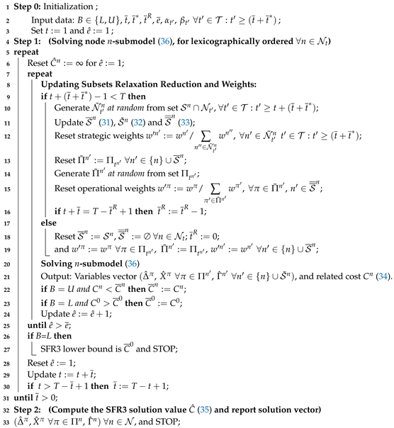
5. SFR3, a Decomposition Matheuristic Algorithm
Fix-and-relax (FR) is a matheuristic algorithm that, to the best of our knowledge, was introduced in [55] for solving dynamic deterministic 0–1 MILP problems. See the same idea described in [56]. It consists of solving a sequential series of subproblems, such that the variables in each one are partitioned into three subsets. The variables in the first subset are fixed, the binary variables in the second one are kept integer, and the integrality of the binary variables in the third subset is relaxed. The partition of the variables results from an ordering which is established a priori, and the variables declared integer in each subproblem define the so-called FR level. In particular, the variables that are fixed at level ℓ are the variables fixed at level plus the variables declared integer in level . However, as a matter of fact, the relaxation of the integrality in a sizable subset of binary variables in the original problem (1)–(30) prevents taking advantage of that integrality feature when solving the submodels in classical FR. Note that the knowledge of the variables’ integrality by any solver strongly helps to model’s tightening by performing probing, fixing variables, eliminating redundant constraints, and appending new cuts. So, the computing effort could be very high for problem solving by straightforward use of the optimizer as well as by using classical FR in the presence of a high number of binary variables in the instance.
Algorithm 1, SFR3, stands for scenario variables fixing and iteratively randomizing the relaxation reduction of the constraints and variables’ integrality. It is a specialization of the FR methodology for partially preventing the drawbacks outlined above. At any iteration but the last one, a given subset of constraints and variables’ integrality is relaxed. After fixing some variables at any iteration, the main idea consists of reducing those relaxations in a set of randomized executions. The rationale behind that scheme in a FR framework consists of keeping the submodels’ dimensions within affordable limits until obtaining a (hopefully, good) feasible solution.
Let the following input parameters and related new sets in SFR3, see Figure 4 and, in particular, the relaxation so-called n-submodel of the original model (1)–(30), for . (A version of that submodel is to be optimized at each modeler-driven execution in the algorithm’s iterations, being related to a subset of the stages in set ):
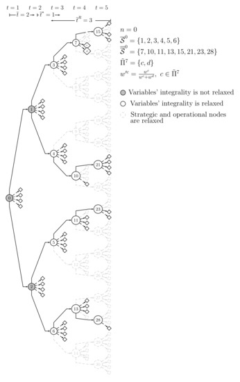
Figure 4.
Strategic multistage scenario tree with operational two-stage scenario trees. SFR3 strategic and operational nodes’ relaxation.
Input parameters
- , number of executions of n-submodel in each iteration of algorithm SFR3.
- , number of consecutive stages (starting with stage t) where no constraints and no variables’ integrality are relaxed while solving the submodels at iteration t.
- , number of the latest consecutive stages , where the relaxation of the variables’ integrality is performed in the n-submodel, say, , provided that relaxation is not performed for stage .
- , additional number of consecutive stages (starting with stage ) where no constraints are relaxed while solving the submodels at iteration t. Note: .
- , probabilities that are allowed for the non-relaxation of operational scenario and strategic nodes, resp., that belong to stage in a execution of n-submodel, see next.
New sets at each execution of n-submodel
- , strategic node subset that belongs to stage whose elements are successors of strategic node n that are not relaxed for solving n-submodel at an execution, for . The nodes in set are selected at random with probability , but with the caveat on keeping a Hamiltonian path from node n to a leaf node in the scenario tree.
- , leaf node set in the strategic subtree rooted at node n up to stage for a given execution of n-submodel. So, . For the purpose of preserving the caveat mentioned above, let the assumption: , such that all nodes, say, , in the Hamiltonian path from a node, say, to a node, say, in the strategic scenario tree, do satisfy the condition , for and . Note that, by construction, node satisfies that condition.
- , operational scenario subset in the two-stage tree rooted at strategic node whose elements are not relaxed for solving n-submodel at an execution, for and as above. The scenarios in set are selected at random with probability .
- , subset of successor nodes of strategic node n that are not a subject for constraints relaxation. It can be expressed as (31).
- , subset of the successor nodes of strategic node n, where the solution of the strategic and related operational variables, jointly with the solutions of the variables in node n and its related operational ones, are retrieved from solving the submodel. Those solutions are partial of the solution for the original model (1)–(30). It can be expressed as (32).
- , subset of the successor nodes in set that have been chosen not to be relaxed in the current execution of the algorithm, for . It can be expressed as (33).
The solution of n-submodel at a given execution of any iteration is denoted as vector . The cost can be expressed
Let denote the smallest cost in the executions of an iteration, and note that is the lower bound of the optimal solution of the original model (1)–(30). Additionally, let be the cost in related to the variables in vector , as a part of the full cost, viz., of the SFR3 solution of the original model to be expressed as
Let denote the input option label, such that means that the aim of the algorithm’s execution is restricted to obtaining a lower bound of the solution value of the original model (1)–(30). On the other hand, means that the aim consists of obtaining a (hopefully, good) feasible solution for the original model, where its solution value is an upper bound of the solution value of the original model.
So, for , the aim of the executions of n-submodel (36), for , consists of providing a (hopefully, good) partial feasible solution, for the original model (1)–(30), at the related iteration, whose cost is (34). That solution is related to the strategic node subset and the set of the operational scenarios . Additionally, the submodel is also included by the constraints and variables supported by the non-relaxed strategic node subset and the non-relaxed set of the operational scenarios . The submodel can be expressed as
Remarks on n-submodel (36): Given the step variable type of the modeling object that is considered for the -variables, only the strategic nodes and n link the submodel (36). Node is such that . So, the solution is retrieved from the -submodel.
| Algorithm 1: SFR3. On obtaining lower and upper bounds on MS-Hub-NEP model (1)–(30). |
 |
Additional Details
- For , is computed as the highest cost (34) in the executions of n-submodel (36) for stage (lines 20 and 23 of the Algorithm 1: SFR3), where . (Recall that, without loss of generality, it is assumed that and ). is a lower bound of the solution value of the original model (1)–(30). Note that the objective function and constraints for node 0 in the n-submodel, jointly with those of its successor nodes in sets (31) and (33) and related operational scenarios, gives a lower bound for each execution.Additionally, observe that the algorithm running is interrupted after obtaining that bound (lines 26–27), so, the input parameters , , , , and could be more restricted than the related values for option .
- For , is computed as the smallest cost in the executions (lines 20–21) of the original model (1)–(30), so that the partial incumbent solution value (line 22) is updated. For that purpose, the scheme in lines 7–25 is used, where n-submodel (36) is solved for all until the updated stage (line 30) is zero. The rationale behind it is that, once the updated stage t (line 29) is such that , then the stages involved in the next iteration are . So, the execution of its Step 1 requires the resetting , and note that it is to be the last iteration of the algorithm. Observe that is reset to zero at the end of its execution.Note 1: The submodel (36) for the full scenario tree rooted at node 0, (i.e., ) is a relaxation of the original model (1)–(30). It is solved for each of the executions.Note 2: The variables related to the ancestor strategic scenario nodes in set are fixed to the values retrieved from the appropriate submodels. In any case, observe that retaining the solution related to the stages t to (that is, fixing it) implies the independence of the submodels supported by the subtrees rooted at the nodes in set .
- The parameters and can have a value of 1. It could be the case where neither strategic, nor operational constraints are relaxed. Observe that the relaxation of the variables’ integrality is allowed for the last stages, so that it is the FR classical algorithm for .
- The weights, say, and (lines 12,15 and 19) to be used in n-submodel (36) for obtaining the SFR3 solution are such that and .
- The strategic node set for and the operational scenario set , for in n-submodel (36), are generated anew in any of the executions, for (lines 10–14). Note: the best solution is retrieved among the executions.
- At Step 1, for a given stage t, such that (line 9), the parameter is reduced to for (line 16). Recall that the parameter is used for deciding the stages where the relaxation of the variables’ integrality is carried out. Moreover, as above, but for , the resetting in lines 18 and 19 is performed, including (i.e., no integer relaxation) and the related weights. Note: in this case, it is assumed that the n-submodels (36) can be solved without further relaxations in an affordable computing time.
6. Computational Experience
This section reports the main computational results that have been obtained while experimenting with a broad testbed composed of a variety of instances from medium MS-Hub-NEP ones up to large-sized instances and very large-sized ones. Section 6.1 presents the instance dimensions and the main parameters used in the experiment. It also gives the structure of the multistage scenario tree under consideration. Section 6.2 presents the dimensions of the related model (1)–(30) and reports the main results that have been obtained by considering CPLEX straightforward use. Section 6.3 presents the strategies that are used by matheuristic SFR3, as well as a comparison of the results.
The computational experiment was conducted on a PC with a 2.9 gigahertz dual-core Intel Core i5 processor, 8 gigabyte of RAM and operating system OS X 10.12.1. The modeling approach, as well as the proposed matheuristic, have been implemented in a C++ experimental code. The default options of CPLEX v20.1.0 are used for the full model (1)–(30) solving, as well as for the n-submodels (36) to be optimized in SFR3. However, given the difficulty of the problem, the optimality tolerance has been set to 1%.
6.1. Testbed Instances
Table 1 shows the dimensions of the instances, under the assumption that the parameter is large enough to allow . The headings for the instances and the structure of the scenario tree are as follows: , instance code; network dimensions: , number of network nodes, it is also the number of candidates hubs in this experiment; , number of network edges, it is also the number of candidate hub links in this experiment; , maximum number of hubs that can be available at any strategic node, so, ; , number of operational scenarios at any stage, so, . The other parameters are as follows: , maximum number of capacity modules that can be installed at any hub, so, ; , maximum number of origin nodes that can be allocated to a hub in any strategic node at any stage, so, ; , number of stages in the time horizon. The dimensions of the strategic scenario tree are as follows, see Figure 3: , number of immediate successor nodes for any strategic node (i.e., ); , number of strategic nodes in the multistage scenario tree; and , number of strategic scenarios (i.e., ). Assumption: The weights and are equiprobable, so, and .

Table 1.
S-Hub-NEP problem. Dimensions.
The number of static stage deterministic hub network expansion planning submodels within the (deterministically equivalent) stochastic full model (1)–(30) is for and for . Those submodels are inter-related by initially sharing hub-network designing -binary variables in the strategic nodes from their immediate ancestor in the scenario tree.
CAB-Inspired Data Generation
The testbed has been partially generated based on the well-known CAB data for deterministic network problems, see [69]. For the experiment with MS-Hub-NEP, a data pattern has been inspired on the two-stage multiperiod data considered in [4]. Accordingly, the hub building setup cost, , has been computed as , where is an ’overall’ flow demand in origin node i.
By taking a 2% increase in the hub building cost from one stage to the next one in the deterministic case, it has been considered in this experiment that , for , where and for the even and odd nodes , resp. Recall that node i is a potential hub, since in this experiment.
The flow demand is computed as the perturbed CAB-based expression
where is the static stage deterministic flow demand for node pair as taken from the CAB data. So, for the operational scenario in the strategic node (i.e., stage ).
The flow capacity K of the modules can be expressed
The installation setup costs of any initial or additional capacity module can be expressed and , resp., . The other cost types are available upon request from the authors.
6.2. CPLEX Straightforward Use. Results
Table 2 shows the model’s dimensions and CPLEX results. The headings for the dimensions are as follows: m, and , number of constraints, binary variables and continuous variables, respectively, and and %, constraint matrix nonzero elements and density, respectively. The headings for the results are as follows: , lower bound of the solution value (i.e., value of the best node in the B&B tree up to the optimization’s interruption); and , incumbent MILP solution value, and its computing time (in seconds, as for all experiments), respectively; and , optimality gap of the incumbent solution, being computed as .
Based on the computational results shown in Table 2, the testbed in Table 1 can be classified into three categories: Cat 1 is included by the middle-scale instances from i1 to i7, whose dimensions are up to m = 175,983 constraints, = 27,156 binary variables and = 134,292 continuous variables; Cat 2 is included by the large-scale instances from i8 to i19, whose dimensions are up to m = 881,643, = 90,706 and = 750,882; and Cat 3 is included by the very large-scale instances from i20 to i32, whose dimensions are up to m = 3,473,631, = 242,172 and = 3,134,844. The computing time limit has been set to 2h for the instances in the categories Cat 1 and Cat 2. Moreover, given the high dimensions of the instances in category Cat 3, the time limit has been set to 15 h.
The solution’s 1% quasi-optimality can not be proved in 4 out of the 7 instances in Cat 1, even considering the model’s tightness (based on the step type of the -,- and -binary variables). Observe that the optimization was interrupted due to the 2 h and 15 h time limitation in all of the instances in Cat 2 and Cat 3, resp. As a matter of fact, that limit was reached while obtaining the lower bound at the B&B root node. The incumbent solution value has been provided by the CPLEX preprocessing heuristic algorithms. Both values contribute to the very high , showing that CPLEX straightforward use is useless. The situation worsens for Cat 3, where usually even no lower bound is obtained at the root node in some instances, since CPLEX is running out of memory in most of them.
6.3. SFR3 Matheuristic. Results
Besides the input parameters , , and presented in Section 5, the elements of the SFR3 strategies for solving the n-submodel (36), supported for a scenario tree rooted at strategic node n, for each of its executions at the iteration coded as stage t, for , are as follows:
- , probability of a scenario not to be relaxed in any operational set for non-relaxed strategic node , where stage starts with along the time horizon, so that is fixed to .
- , probability of a strategic node not to be relaxed, where stage starts with along the time horizon, so that is fixed to .
The following four SFR3 strategies are considered in decreasing relaxation order:
stra = 1: Strong myopic. It consists of a myopic one stage-based rolling horizon approach, where the submodel supported by a subtree rooted at strategic node n, is included by the constraints and variables that only belong to that node as well as the related scenarios in operational set . Its components are , , , and , Note that the scheme for the latest consecutive stages for variables’ integrality relaxation does not apply here. Once the solution is fixed, the algorithm proceeds to update .
stra = 2: Weaker myopic. It consists of a myopic two stage-based rolling horizon approach, where (a) The model, supported by a subtree rooted at strategic node n, is included by the constraints and variables that belong to that node n and its immediate successors (i.e., set ) as well as the related scenarios in the operational sets , for ; and
(b) The variables’ integrality is relaxed in the node sets and . Its components are , , , and . By convention, means that the variables’ integrality relaxation is restricted to the number of consecutive stages starting at stage , and in this case finishing at it, (i.e., the next one to stage t in this experiment). Once the solution is fixed, the algorithm proceeds to update .
stra = 3: Scenario variables Fixing and variables’ integrality iteratively Relaxation Reduction in the given latest consecutive stages . By construction, no constraints are relaxed. Its components are , , , and , since in this experiment. Note: .
stra = 4: Scenario variables Fixing and iteratively Randomizing the Relaxation Reduction of the constraints and variables’ integrality, for chosen .
The computing time limit has been set to 2 h for each execution of submodel (36) in any iteration of the strategies.
For assessing the performance of the SFR3 strategies, Table 3 reports the aggregation by categories Cat 1, Cat 2 and Cat 3 of the instances’ results. The new headings are as follows: , , , , , average and standard deviation of the cost of the SFR3 incumbent solution , average of the optimality gap , average of the computing time , and average of the goodness ratio , resp. All the instances’ results are taken from Table A1, but that is computed as , where the lower bound is taken from Table 4. For comparative purposes, it is also shown for each category. It stands for the average cost of the CPLEX incumbent solution in the instances as taken from Table 2.
It can be observed in Table 3 that strategy stra = 4 obtains an incumbent solution value very similar for category Cat 1 to the one obtained by CPLEX straightforward. On the other hand, it is the champion for medium- and large-scale instances (i.e., categories Cat 1 and Cat 2, resp.). Note that the higher the pair , the smaller the expected cost of the incumbent solution in the scenarios. An important observation is that SFR3 provides a lower bound, such that the optimality gap for the best pair is around 6%.
Table 4 shows the results obtained for the best of the four strategies (i.e., the one with the smaller solution value), whose computational comparison is shown in Table A1, see Appendix B. The headings are as follows: -, instance code-strategy, where goes from 1 to 4; and , lower bound of the solution value of model (1)–(30) obtained by SFR3 in an independent run to that based on the chosen strategy (see below), and computing time, resp.; , and , incumbent solution value (i.e., smallest ’expected’ cost (35) in the scenarios), median obtained by SFR3 in the set of executions that have been carried out for each n-submodel (36), and overall computing time that is required, resp., for the whole set of the executions; , optimality gap of the best SFR3 incumbent solution , being computed as ; and , goodness ratio of the SFR3 best incumbent solution over the CPLEX one, being computed as . Note: the smaller the goodness ratio , the better performance of SFR3 versus CPLEX straightforward use.
Remark. The lower bound provided by SFR3 can be very weak for small values of pair . So, is the related lower bound of (i.e., the classical fix-and-relax approach), independently of its ability for obtaining a feasible solution for the original model (1)–(30). It is the lower bound of the solution value of the model attached to strategic node (i.e., at its iteration ). For that purpose, 2 h time limit has been imposed for instances in Cap 1 and Cap 2, and 4 h is the time limit for the instances in Cap 3. Note: means that no solution has been obtained in the B&B root node within the time allowed, as in instances i26, i27, i29 and i32.
Observe that the optimality gap allowed 1% is also satisfied by SFR3 for the instances i1, i2 and i3. Additionally, the solutions obtained by SFR3 are very close to the CPLEX ones for the other members of Cat 1. Probably, it is an indication of the quality of SFR3 as a solution provider. On the other hand, note that all of the 32 instances in the testbed have been solved by matheuristic SFR3, where the strategies , usually, provide comparable solutions with the CPLEX ones for the instances in Cat 1, see the goodness ratio , requiring very little computing time. On the other hand, SFR3 consistently provides much better solutions for the instances with higher dimensions. It can also be observed that strategy provides the best solution for most of the instances. However, strategy gives the best solution value of 9 out of the 32 instances in the testbed within a reasonable computing time. Additionally, note that the myopic strategies were needed for two of the most difficult instances, for i32 and even for i29. Observe also the weakness of the lower bound for the instances in Cat 3, if any, reaching the time allowed in all of them. Moreover, note also that the goodness ratio is very small for the instances where CPLEX straightforward use provides a feasible solution; it is below 0.04 for most of the instances in Cat 2 and Cat 3, which is an impressive result obtained by SFR3 versus CPLEX straightforward use; the problem is so difficult that it is hopeless, except for Cat 1.
It can be observed in Appendix B that the median cost in the 10 and 5 executions is very close to the incumbent one in most of the instances when strategy SFR3 is considered. Obviously, it means that at least 50% of the executions give very close costs to the incumbent one. So, besides those statistics, it is also important to consider the cost distribution in the set of the executions, instead of just considering the expected one for some values of pair . For that purpose, Figure 5 depicts the boxplot for the ’expected’ cost (35) distribution as well as the median in the executions for instance i6; all of those costs are generally named . By construction, strategies only have execution, so, the median is the same cost. On the other hand, executions have been carried out for strategy . Note the impact of considering the two-stage myopic strategy versus the one-stage . The randomized relaxation reduction related strategy (where ) provides a solution with the smallest median.
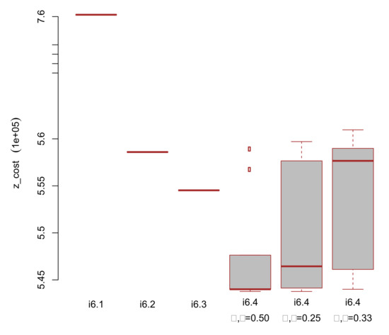
Figure 5.
Instance i6. SFR3 strategies comparison. Cost distribution and median in executions.
7. Conclusions
In this work, a mixed integer linear optimization model is presented for the capacitated hub network expansion planning problem, MS-Hub-NEP, in a multistage multiscale framework under uncertainty. Two types of uncertainties are considered. Both are represented in finite sets of scenarios. The first type is related to the costs of the hub building and initial capacity modules and extensions at the strategic nodes of a multistage scenario tree; it is assumed to be stagewise-dependent and, then, it is attached to each strategic node and influences its successors. The strategic variables have been modeled by considering the step modeling object a tighter approach than its impulse counterpart. Additionally, it is very appropriate for the decomposition matheuristic algorithm SFR3 that is also introduced in this work. In contrast, the second type of uncertainty is related to the hub network operation and, then, it is only stage-dependent. It represents the stage flow demand and cost of flow hub allocation, collection, transfer and non-stop service from origin to destination. A two-stage tree rooted at the strategic nodes is considered for representing the operational scenarios.
MS-Hub-NEP is very difficult to solve, even for medium-scale instances. CPLEX straightforward use could only guarantee the solution’s 1% quasi-optimality in the three smallest instances in the experiment that has been carried out, being composed by 32 instances. As a matter of fact, its straightforward use is hopeless for large- and very large-scale instances, where the execution is interrupted when reaching the computing time limit, 2 h and 15 h, resp. The number of hubs, hub edges, stages and strategic nodes for each instance go from 4, 12, 5, 31 to 20, 380, 5, 31, resp., the operational scenarios are 4 and 8 per stage depending on the instance, and the number of constraints, binary variables and continuous variables are 3,473,631, 242,172 and 3,134,844, resp.
The matheuristic SFR3 provides a solution for all of the 32 instances in the testbed. Two of the four strategies that have been experimented with are one-stage and two-stage myopic rolling time horizon-based approaches. They are a benchmark for the other two strategies as well as for solving 2 out of the 13 very large-scale instances; the computing time is affordable. The third strategy is the well-known Fix-and-Relax approach. Its usefulness for solving MS-Hub-NEP has been empirically proven in this experiment, provided that the hardware/software resources allow to solve the n-submodel (36) at the first iteration . The fourth strategy deals with the scheme for iteratively Randomizing the Relaxation Reduction of constraints and variables’ integrality for solving MS-Hub-NEP; it could be expanded without much difficulty to solving other stochastic multistage multiscale problems. The - and -mechanisms for selecting operational scenarios and strategic nodes, resp., not to be relaxed in each execution of the submodel to be solved at each iteration of the decomposition approach, have shown to be very efficient for solving this very challenging HLP. The strategy is very flexible and its roots go back to the third strategy; on the other hand, the optimality gap of the attained incumbent solution is reasonable. The strategy usually provides the best results, within affordable computational resources. It outperforms CPLEX straightforward use for large and very large instances (i.e., categories Cat 2 and Cat 3). Note that the solution values of CPLEX and SFR3 are very similar for the medium scale instances Cat 1.
Anyway SFR3 provides the lower bound of the solution value by considering the third strategy for stage . Its optimality gap is around 6% for most of the instances.
7.1. Outline of Perspectives and Future Research Agenda
The structure of the model MS-Hub-NEP (1)–(30) can be considered on other types of system or network expansion problems as the facility location and expansion planning [68] and, in a more general setting, the distributional robust optimization multistage multiscale stochastic problems [70]. The proposed matheuristic methodology, including its scheme for obtaining lower bounds and the potentiality for considering multi-objective functions, could be extrapolated to solve other multistage multiscale MILP as those ones, among others, in a similar way as in [62].
The features of the strategic nodes and the operational scenario submodels that would extend the proposed model as items in a research agenda are as follows: In the strategic node submodel: (a) a moderate additional number of hubs to the two, at most, that right now are considered for any origin-destination flow, (b) strategic uncertainty on the (total or full) unavailability of hub edges and hubs themselves, due to disfunction interruptions; and (c) allowing the possibility of hub leasing for given stages. In the operational scenario submodels: operational uncertainty on the (total or full) unavailability of hub edges and hubs themselves, due to temporal interruptions in the stages. Those features may substantially increase the model’s high dimensions, due to the higher cardinality of the operational scenario sets and additional strategic constraints. However, it seems that those modifications can be accepted by the algorithm SFR3 as it is, given its generality.
In any case, note that the computing time that is required by strategies is relatively high for solving the n-submodel (36) for the set included by the first stages, even for . So, that difficulty precludes the exclusion of decomposition algorithms that require the optimal solution of even one single scenario submodel as e.g., those approaches based on scenario Lagrangean decomposition, see [49]. Probably, given the character of the state step variables, the Stochastic Nested Decomposition (SND) research would take benefit from the splitting variable scheme introduced in [51] for state binary variables, see also [50]. As a matter of fact, it does not require solving any full scenario submodel. So, it could be interesting to computationally compare the performance of SND against the proposed matheuristic SFR3 alone, as well as considering it in the Front-to-Back step of the first SND iteration.
Author Contributions
Conceptualization, L.F.E. and J.F.M.; Formal analysis, L.F.E.; Methodology, L.F.E. and J.F.M.; Software, J.F.M.; Writing—original draft, L.F.E.; Writing—review & editing, J.F.M. All authors have read and agreed to the published version of the manuscript.
Funding
This research was funded by the grant PID2019-105952GB-I00 funded by Ministerio de Ciencia e Innovación/Agencia Estatal de Investigación /10.13039/501100011033 and the grant RTI2018-094269-B-I00 funded by Ministerio de Ciencia e Innovación/Agencia Estatal de Investigación.
Data Availability Statement
Not applicable.
Acknowledgments
The authors appreciate and wish to thank to Juan José Peiró for his reading of an earlier version of the work and, in particular, his observations on the uncapacitated version of the problem. They also appreciate the positive criticism of the reviewers for their help on improving the contents and presentation of the work.
Conflicts of Interest
The authors declare no conflict of interest.
Appendix A. Illustrative Example
Figure A1 depicts an example to illustrate the main decisions to made in MS-Hub-NEP and the role of the scenario strategic nodes and operational scenarios in a network whose infrastructure is new for three-stages in a time horizon. It is assumed that are the network nodes.
Appendix A.1. Strategic and Operational Decisions
The strategic nodes under consideration are at stage , at stage , and at stage in the scenario tree depicted in Figure 3. Based on the hub building and capacity module costs in the strategic nodes as well as the flow demand and transportation costs under the operational scenarios, the strategic decisions are assumed to be made as follows: for , hubs 1 and 3 building with given initial capacity modules; for , hub 1 capacity expansion with given additional modules, and hub 2 building with given initial capacity modules; and for , hub 2 capacity expansion with given additional modules.
The figure also shows the operational decisions that have been assumed for each of those strategic nodes under given scenarios in the operational set , for . Those decisions are related to transporting the flow demand from origin to destination. That is, it shows the routes , or , for the flow of each network node pair under the operational scenario in assumed in the example for the strategic node set under consideration. Recall that denotes the non-stop service mode for node pair , so that in case of occurring then the other routes are prevented. For saving space purposes, let us assume that the operational decisions that have been made for strategic node are as the ones considered in Figure 1, so that they have been brought to Figure A1. The operational decisions for the strategic nodes and in the example are also depicted in the figure. Observe that it is assumed that hub 1 is outbound under the given operational scenario related to strategic node , being the origin of a portion of the flow demand to destination node 5.
Strategic variables for hub k in strategic nodes
- For node :
- -
- .
- -
- , where e.g., initial capacity module, and , where e.g., .
- For node :
- -
- .
- -
- , and , where e.g., initial capacity module.
- -
- , where e.g., additional capacity modules.
- For node :
- -
- .
- -
- , where e.g., additional capacity modules.
Operational variables for a given scenario in each strategic node
- For node :
- -
- .
- -
- , , , , , .
- -
- , , .
- -
- , , , , , .
Note: Hub 3 is a flow inbound from origin node 8. - For node :
- -
- , , , , , , , , , .
- -
- , , , , , , .
- -
- , , , , , , , , .
- For node :
- -
- , , , , , , , , , .
- -
- , , , , , , .
- -
- , , , , , , , .
- -
- .
Note: Hub 1 is a flow outbound to destination node 5.
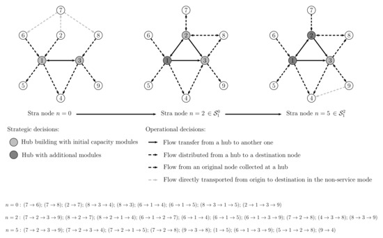
Figure A1.
Origin and destination network nodes and hubs representation. Strategic and operational decisions.
Appendix B. Computational Comparison of the SFR3 Strategies stra = 1,2,3,4
Table A1 reports information about the behavior of different values for pair in strategy . In particular, the values are (0.50, 0.50), (0.33, 033) and (0.25, 0.25). The additional headings are as follows: , instance code - strategy, where goes from 1 to 4; , and , incumbent solution value (i.e., the smallest ’expected’ cost (31) in the scenarios), median obtained by SFR3 in the set of executions that have been carried out for the probability pair in each n-submodel (36), and overall computing time that is required by the whole set of executions, resp.; and , goodness ratio of the SFR3 incumbent solution over the CPLEX one, being computed as , where the smaller , the better performance of SFR3 versus CPLEX straightforward use.
It is worth to point out that it is required to increase the randomized relaxation fraction up to for some of the most difficult instances, say i31 and i32.
Observe also that the SFR3 strategies usually provide comparable solutions with the CPLEX straightforward use for the instances in Cat 1, see the goodness ratio , requiring very small computing time. On the other hand, SFR3 consistently provides much better solutions for the instances with higher dimensions. Note that in most of the instances the goodness ratio is below 0.04, which is an impressive result for SFR3 versus CPLEX straightforward use. On the other hand, it requires an affordable computing time up to instance i22, being usually smaller than the one allowed for CPLEX straightforward use. No solution is provided by the latter for most of the difficult problems in Cat 3. However, the strategies do provide the best solution value, but for instances i29 and i32 where give a better solution in a much smaller computing time.
As a reminder, SFR3 strategy is the classical Fix-and-Relax, which does not provide any solution for instances i25, i31 and i32, see Table A1. The main reason is that CPLEX cannot solve n-submodel (36) at iteration ; note that the variables’ integrality is relaxed for some of the submodels. On the other hand, note that it could happen that CPLEX straightforward use (for the full model) does provide a solution for the same instance. The main reason in large-scale instances is that CPLEX -as well as other state-of-the-art solvers- use the available information on the variables’ integrality. For the straightforward use of the solver, it is the information on all of the binary variables from the first stage to the last. By contrast, CPLEX in SFR3 strategy does only use the information on the variables’ integrality of the strategic nodes where the solution is sought for (i.e., set and related sets ), while the variables’ integrality for the other successor nodes has been relaxed. However, observe that the model dimensions for CPLEX straightforward use could be increased by appending the additional cuts generated by the integrality implications detected in the preprocessing phase. Thus, that increase in the model could prevent attaining solutions at the B&B root node when the computer memory and time requirements are up to the imposed limitations, as it is the case for the testbed in the experiment. As an example, SFR3 gives the incumbent solution value = 494,044 for instance i10, requiring seconds. CPLEX straightforward use could not provide a solution at the B&B root node in the 2h time limit, but the lower bound = 472,112 and, on the other hand, = 2,266,526 is the very bad solution obtained by the CPLEX preprocessing heuristics; see Table 2 in the main body of the paper. Thus, .
It can be observed for SFR3 that the median cost in the 5 and 10 executions is very close to the incumbent in most of the instances. Obviously, it means that at least 50% of the executions give very close costs to the incumbent one. So, besides those statistics, it is also important to consider the cost distribution in the set of the executions, instead of just the expected one for some values of pair . For clarification purposes, see Figure A1 above.
| i1.1 | 1 | 0 | 0.00 | 0.00 | – | 1 | 566419 | – | 2 | 1.71 |
| i1.2 | 1 | 1 | 0.00 | 0.00 | (*) | 1 | 568971 | – | 1 | 1.72 |
| i1.3 | 1 | 4 | 1.00 | 1.00 | 4 | 1 | 332254 | – | 9 | 1.00 |
| i1.4 | 1 | 1 | 0.50 | 0.50 | 4 | 10 | 331183 | 396499 | 31 | 1.00 |
| i1.4 | 1 | 1 | 0.33 | 0.33 | 4 | 10 | 395593 | 433559 | 17 | 1.20 |
| i1.4 | 1 | 1 | 0.25 | 0.25 | 4 | 10 | 395497 | 434082 | 16 | 1.20 |
| i2.1 | 1 | 0 | 0.00 | 0.00 | – | 1 | 354618 | – | 2 | 1.05 |
| i2.2 | 1 | 1 | 0.00 | 0.00 | (*) | 1 | 339152 | – | 3 | 1.01 |
| i2.3 | 1 | 4 | 1.00 | 1.00 | 4 | 1 | 337364 | – | 14 | 1.00 |
| i2.4 | 1 | 1 | 0.50 | 0.50 | 4 | 10 | 345266 | 345685 | 52 | 1.03 |
| i2.4 | 1 | 1 | 0.33 | 0.33 | 4 | 10 | 345300 | 352808 | 32 | 1.03 |
| i2.4 | 1 | 1 | 0.25 | 0.25 | 4 | 10 | 326391 | 328097 | 29 | 0.97 |
| i3.1 | 1 | 0 | 0.00 | 0.00 | – | 1 | 913829 | – | 6 | 2.59 |
| i3.2 | 1 | 1 | 0.00 | 0.00 | (*) | 1 | 588399 | – | 4 | 1.66 |
| i3.3 | 1 | 4 | 1.00 | 1.00 | 4 | 1 | 354955 | – | 55 | 1.00 |
| i3.4 | 1 | 1 | 0.50 | 0.50 | 4 | 10 | 355073 | 355132 | 212 | 1.00 |
| i3.4 | 1 | 1 | 0.33 | 0.33 | 4 | 10 | 355073 | 552572 | 116 | 1.00 |
| i3.4 | 1 | 1 | 0.25 | 0.25 | 4 | 10 | 501339 | 501339 | 5 | 1.42 |
| i4.1 | 1 | 0 | 0.00 | 0.00 | – | 1 | 589659 | – | 8 | 1.01 |
| i4.2 | 1 | 1 | 0.00 | 0.00 | (*) | 1 | 403383 | – | 5 | 1.01 |
| i4.3 | 1 | 4 | 1.00 | 1.00 | 4 | 1 | 397350 | – | 34 | 1.01 |
| i4.4 | 1 | 1 | 0.50 | 0.50 | 4 | 10 | 395607 | 396156 | 130 | 1.01 |
| i4.4 | 1 | 1 | 0.33 | 0.33 | 4 | 10 | 395607 | 403383 | 72 | 1.01 |
| i4.4 | 1 | 1 | 0.25 | 0.25 | 4 | 10 | 395607 | 403383 | 64 | 1.01 |
| i5.1 | 1 | 0 | 0.00 | 0.00 | – | 1 | 407646 | – | 34 | 1.26 |
| i5.2 | 1 | 1 | 0.00 | 0.00 | (*) | 1 | 409952 | – | 35 | 1.27 |
| i5.3 | 1 | 4 | 1.00 | 1.00 | 4 | 1 | 326541 | – | 52 | 1.01 |
| i5.4 | 1 | 1 | 0.50 | 0.50 | 4 | 10 | 325288 | 326905 | 397 | 1.01 |
| i5.4 | 1 | 1 | 0.33 | 0.33 | 4 | 10 | 325711 | 328035 | 263 | 1.01 |
| i5.4 | 1 | 1 | 0.25 | 0.25 | 4 | 10 | 326391 | 328097 | 210 | 1.01 |
| i6.1 | 1 | 0 | 0.00 | 0.00 | – | 1 | 763196 | – | 6 | 1.42 |
| i6.2 | 1 | 1 | 0.00 | 0.00 | (*) | 1 | 558594 | – | 7 | 1.04 |
| i6.3 | 1 | 4 | 1.00 | 1.00 | 4 | 1 | 554524 | – | 73 | 1.03 |
| i6.4 | 1 | 1 | 0.50 | 0.50 | 4 | 10 | 543769 | 544002 | 481 | 1.01 |
| i6.4 | 1 | 1 | 0.33 | 0.33 | 4 | 10 | 543770 | 545249 | 197 | 1.01 |
| i6.4 | 1 | 1 | 0.25 | 0.25 | 4 | 10 | 544002 | 557659 | 169 | 1.01 |
| i7.1 | 1 | 0 | 0.00 | 0.00 | – | 1 | 473378 | – | 22 | 1.26 |
| i7.2 | 1 | 1 | 0.00 | 0.00 | (*) | 1 | 384915 | – | 19 | 1.03 |
| i7.3 | 1 | 4 | 1.00 | 1.00 | 4 | 1 | 381308 | – | 249 | 1.02 |
| i7.4 | 1 | 1 | 0.50 | 0.50 | 4 | 10 | 379276 | 381240 | 840 | 1.01 |
| i7.4 | 1 | 1 | 0.33 | 0.33 | 4 | 10 | 380610 | 420863 | 425 | 1.01 |
| i7.4 | 1 | 1 | 0.25 | 0.25 | 4 | 10 | 380147 | 453920 | 301 | 1.01 |
| i8.1 | 1 | 0 | 0.00 | 0.00 | – | 1 | 1077627 | – | 6 | 1.31 |
| i8.2 | 1 | 1 | 0.00 | 0.00 | (*) | 1 | 842510 | – | 18 | 1.02 |
| i8.3 | 1 | 4 | 1.00 | 1.00 | 4 | 1 | 816346 | – | 65 | 0.99 |
| i8.4 | 1 | 1 | 0.50 | 0.50 | 4 | 10 | 817379 | 842510 | 860 | 0.99 |
| i8.4 | 1 | 1 | 0.33 | 0.33 | 4 | 10 | 816947 | 842543 | 430 | 0.99 |
| i8.4 | 1 | 1 | 0.25 | 0.25 | 4 | 10 | 842510 | 965237 | 340 | 1.02 |
| i9.1 | 1 | 0 | 0.00 | 0.00 | – | 1 | 1113515 | – | 12 | 0.23 |
| i9.2 | 1 | 1 | 0.00 | 0.00 | (*) | 1 | 1058052 | – | 45 | 0.22 |
| i9.3 | 1 | 4 | 1.00 | 1.00 | 4 | 1 | 967824 | – | 394 | 0.20 |
| i9.4 | 1 | 1 | 0.50 | 0.50 | 4 | 10 | 968313 | 985627 | 5083 | 0.20 |
| i9.4 | 1 | 1 | 0.33 | 0.33 | 4 | 10 | 984841 | 990246 | 1664 | 0.20 |
| i9.4 | 1 | 1 | 0.25 | 0.25 | 4 | 10 | 985445 | 1008011 | 1210 | 0.20 |
| i10.1 | 1 | 0 | 0.00 | 0.00 | – | 1 | 518999 | – | 21 | 0.23 |
| i10.2 | 1 | 1 | 0.00 | 0.00 | (*) | 1 | 496106 | – | 41 | 0.22 |
| i10.3 | 1 | 4 | 1.00 | 1.00 | 4 | 1 | 494044 | – | 412 | 0.22 |
| i10.4 | 1 | 1 | 0.50 | 0.50 | 4 | 10 | 493947 | 495048 | 1776 | 0.22 |
| i10.4 | 1 | 1 | 0.33 | 0.33 | 4 | 10 | 493947 | 556325 | 827 | 0.22 |
| i10.4 | 1 | 1 | 0.25 | 0.25 | 4 | 10 | 494865 | 521692 | 713 | 0.22 |
| i11.1 | 1 | 0 | 0.00 | 0.00 | – | 1 | 1493974 | – | 240 | 0.92 |
| i11.2 | 1 | 1 | 0.00 | 0.00 | (*) | 1 | 1311741 | – | 168 | 0.81 |
| i11.3 | 1 | 4 | 1.00 | 1.00 | 4 | 1 | 1215811 | – | 334 | 0.75 |
| i11.4 | 1 | 1 | 0.50 | 0.50 | 4 | 10 | 1211605 | 1221856 | 4680 | 0.74 |
| i11.4 | 1 | 1 | 0.33 | 0.33 | 4 | 10 | 1211701 | 1221856 | 2091 | 0.74 |
| i11.4 | 1 | 1 | 0.25 | 0.25 | 4 | 10 | 1211715 | 1311799 | 1908 | 0.74 |
| i12.1 | 1 | 0 | 0.00 | 0.00 | – | 1 | 929879 | – | 99 | 0.04 |
| i12.2 | 1 | 1 | 0.00 | 0.00 | (*) | 1 | 900970 | – | 96 | 0.04 |
| i12.3 | 1 | 4 | 1.00 | 1.00 | 4 | 1 | 743000 | – | 643 | 0.03 |
| i12.4 | 1 | 1 | 0.50 | 0.50 | 4 | 10 | 742986 | 743665 | 2750 | 0.03 |
| i12.4 | 1 | 1 | 0.33 | 0.33 | 4 | 10 | 743013 | 872369 | 1524 | 0.03 |
| i12.4 | 1 | 1 | 0.25 | 0.25 | 4 | 10 | 743054 | 769487 | 1232 | 0.03 |
| i13.1 | 1 | 0 | 0.00 | 0.00 | – | 1 | 2004808 | – | 147 | 0.04 |
| i13.2 | 1 | 1 | 0.00 | 0.00 | (*) | 1 | 1336341 | – | 146 | 0.03 |
| i13.3 | 1 | 4 | 1.00 | 1.00 | 4 | 1 | 1262833 | – | 4953 | 0.03 |
| i13.4 | 1 | 1 | 0.25 | 0.25 | 4 | 5 | 1287213 | 1340038 | 1295 | 0.03 |
| i14.1 | 1 | 0 | 0.00 | 0.00 | – | 1 | 1072064 | – | 121 | 0.03 |
| i14.2 | 1 | 1 | 0.00 | 0.00 | (*) | 1 | 870620 | – | 112 | 0.02 |
| i14.3 | 1 | 4 | 1.00 | 1.00 | 4 | 1 | 874675 | – | 1467 | 0.02 |
| i14.4 | 1 | 1 | 0.50 | 0.50 | 4 | 10 | 868283 | 874675 | 8534 | 0.02 |
| i14.4 | 1 | 1 | 0.33 | 0.33 | 4 | 10 | 869989 | 873346 | 3470 | 0.02 |
| i14.4 | 1 | 1 | 0.25 | 0.25 | 4 | 10 | 869750 | 873346 | 2745 | 0.02 |
| i15.1 | 1 | 0 | 0.00 | 0.00 | – | 1 | 4748345 | – | 158 | 0.06 |
| i15.2 | 1 | 1 | 0.00 | 0.00 | (*) | 1 | 3378703 | – | 114 | 0.04 |
| i15.3 | 1 | 4 | 1.00 | 1.00 | 4 | 1 | 3299658 | – | 2961 | 0.04 |
| i15.4 | 1 | 1 | 0.25 | 0.25 | 4 | 5 | 3376770 | 3521995 | 1273 | 0.04 |
| i16.1 | 1 | 0 | 0.00 | 0.00 | – | 1 | 1322785 | – | 373 | 0.03 |
| i16.2 | 1 | 1 | 0.00 | 0.00 | (*) | 1 | 1314440 | – | 317 | 0.03 |
| i16.3 | 1 | 4 | 1.00 | 1.00 | 4 | 1 | 1105696 | – | 3056 | 0.02 |
| i16.4 | 1 | 1 | 0.50 | 0.50 | 4 | 10 | 1115006 | 1118602 | 9982 | 0.02 |
| i16.4 | 1 | 1 | 0.33 | 0.33 | 4 | 10 | 1110520 | 1127188 | 5573 | 0.02 |
| i16.4 | 1 | 1 | 0.25 | 0.25 | 4 | 10 | 1108419 | 1188678 | 4631 | 0.02 |
| i17.1 | 1 | 0 | 0.00 | 0.00 | – | 1 | 4765528 | – | 216 | 0.06 |
| i17.2 | 1 | 1 | 0.00 | 0.00 | (*) | 1 | 3840918 | – | 169 | 0.05 |
| i17.3 | 1 | 4 | 1.00 | 1.00 | 4 | 1 | 3498342 | – | 5640 | 0.04 |
| i17.4 | 1 | 1 | 0.25 | 0.25 | 4 | 5 | 3470274 | 3634862 | 1790 | 0.04 |
| i18.1 | 1 | 0 | 0.00 | 0.00 | – | 1 | 5563198 | – | 496 | 0.05 |
| i18.2 | 1 | 1 | 0.00 | 0.00 | (*) | 1 | 4998428 | – | 287 | 0.05 |
| i18.3 | 1 | 4 | 1.00 | 1.00 | 4 | 1 | 4919158 | – | 7323 | 0.05 |
| i18.4 | 1 | 1 | 0.25 | 0.25 | 4 | 5 | 4376836 | 4703839 | 5665 | 0.04 |
| i19.1 | 1 | 0 | 0.00 | 0.00 | – | 1 | 1435743 | – | 737 | 0.02 |
| i19.2 | 1 | 1 | 0.00 | 0.00 | (*) | 1 | 1214774 | – | 262 | 0.02 |
| i19.3 | 1 | 4 | 1.00 | 1.00 | 4 | 1 | 1192122 | – | 7513 | 0.02 |
| i19.4 | 1 | 1 | 0.25 | 0.25 | 4 | 5 | 1305792 | 1329767 | 4247 | 0.02 |
| i20.1 | 1 | 0 | 0.00 | 0.00 | – | 1 | 5509216 | – | 565 | 0.05 |
| i20.2 | 1 | 1 | 0.00 | 0.00 | (*) | 1 | 5376021 | – | 620 | 0.05 |
| i20.3 | 1 | 4 | 1.00 | 1.00 | 4 | 1 | 5250293 | – | 7454 | 0.04 |
| i20.4 | 1 | 1 | 0.25 | 0.25 | 4 | 5 | 4677596 | 5117283 | 8211 | 0.04 |
| i21.1 | 1 | 0 | 0.00 | 0.00 | – | 1 | 4420856 | – | 1219 | 0.04 |
| i21.2 | 1 | 1 | 0.00 | 0.00 | (*) | 1 | 3576249 | – | 545 | 0.03 |
| i21.3 | 1 | 4 | 1.00 | 1.00 | 4 | 1 | 3574363 | – | 7509 | 0.03 |
| i21.4 | 1 | 1 | 0.25 | 0.25 | 4 | 5 | 3460527 | 3713737 | 3814 | 0.03 |
| i22.1 | 1 | 0 | 0.00 | 0.00 | – | 1 | 6062626 | – | 434 | 0.05 |
| i22.2 | 1 | 1 | 0.00 | 0.00 | (*) | 1 | 6199723 | – | 789 | 0.05 |
| i22.3 | 1 | 4 | 1.00 | 1.00 | 4 | 1 | 6195805 | – | 7505 | 0.05 |
| i22.4 | 1 | 1 | 0.25 | 0.25 | 4 | 5 | 5647473 | 5885361 | 12152 | 0.04 |
| i23.1 | 1 | 0 | 0.00 | 0.00 | – | 1 | 4810217 | – | 922 | 0.04 |
| i23.2 | 1 | 1 | 0.00 | 0.00 | (*) | 1 | 3921690 | – | 891 | 0.03 |
| i23.3 | 1 | 4 | 1.00 | 1.00 | 4 | 1 | 3868223 | – | 7643 | 0.03 |
| i23.4 | 1 | 1 | 0.25 | 0.25 | 4 | 5 | 3884956 | 4092853 | 6036 | 0.03 |
| i24.1 | 1 | 0 | 0.00 | 0.00 | – | 1 | 10874201 | – | 1680 | – |
| i24.2 | 1 | 1 | 0.00 | 0.00 | (*) | 1 | 10126557 | – | 728 | – |
| i24.3 | 1 | 4 | 1.00 | 1.00 | 4 | 1 | 9772910 | – | 7651 | – |
| i24.4 | 1 | 1 | 0.25 | 0.25 | 4 | 5 | 9766088 | 10115514 | 19097 | – |
| i25.1 | 1 | 0 | 0.00 | 0.00 | – | 1 | 5362888 | – | 1847 | 0.04 |
| i25.2 | 1 | 1 | 0.00 | 0.00 | (*) | 1 | 5132699 | – | 967 | 0.04 |
| i25.3 | 1 | 4 | 1.00 | 1.00 | 4 | 1 | – | – | – | – |
| i25.4 | 1 | 1 | 0.25 | 0.25 | 4 | 5 | 4842158 | 4973660 | 11256 | 0.03 |
| i26.1 | 1 | 0 | 0.00 | 0.00 | – | 1 | 11346333 | – | 3507 | – |
| i26.2 | 1 | 1 | 0.00 | 0.00 | (*) | 1 | 10986554 | – | 3750 | – |
| i26.3 | 1 | 4 | 1.00 | 1.00 | 4 | 1 | 11525857 | – | 7724 | – |
| i26.4 | 1 | 1 | 0.25 | 0.25 | 4 | 5 | 10634810 | 11670300 | 54606 | – |
| i27.1 | 1 | 0 | 0.00 | 0.00 | – | 1 | 12020554 | – | 3354 | – |
| i27.2 | 1 | 1 | 0.00 | 0.00 | (*) | 1 | 10550018 | – | 3900 | – |
| i27.3 | 1 | 4 | 1.00 | 1.00 | 4 | 1 | 11440102 | – | 7908 | – |
| i27.4 | 1 | 1 | 0.25 | 0.25 | 4 | 5 | 10515986 | 11979699 | 44680 | – |
| i28.1 | 1 | 0 | 0.00 | 0.00 | – | 1 | 6619515 | – | 2151 | 0.04 |
| i28.2 | 1 | 1 | 0.00 | 0.00 | (*) | 1 | 5403491 | – | 2035 | 0.03 |
| i28.3 | 1 | 4 | 1.00 | 1.00 | 4 | 1 | 5720090 | – | 7839 | 0.04 |
| i28.4 | 1 | 1 | 0.25 | 0.25 | 4 | 5 | 4848022 | 5141084 | 16810 | 0.03 |
| i29.1 | 1 | 0 | 0.00 | 0.00 | – | 1 | 11586305 | – | 5483 | – |
| i29.2 | 1 | 1 | 0.00 | 0.00 | (*) | 1 | 11604908 | – | 10514 | – |
| i29.3 | 1 | 4 | 1.00 | 1.00 | 4 | 1 | 12551581 | – | 13282 | – |
| i29.4 | 1 | 1 | 0.25 | 0.25 | 4 | 5 | 11978319 | 39568606 | 61395 | – |
| i30.1 | 1 | 0 | 0.00 | 0.00 | – | 1 | 7019432 | – | 3298 | – |
| i30.2 | 1 | 1 | 0.00 | 0.00 | (*) | 1 | 6241369 | – | 5616 | – |
| i30.3 | 1 | 4 | 1.00 | 1.00 | 4 | 1 | 5510879 | – | 7975 | – |
| i30.4 | 1 | 1 | 0.25 | 0.25 | 4 | 5 | 5199642 | 5568422 | 30977 | – |
| i31.1 | 1 | 0 | 0.00 | 0.00 | – | 1 | 9454280 | – | 5650 | – |
| i31.2 | 1 | 1 | 0.00 | 0.00 | (*) | 1 | 8762868 | – | 10895 | – |
| i31.3 | 1 | 4 | 1.00 | 1.00 | 4 | 1 | – | – | – | – |
| i31.4 | 1 | 1 | 0.16 | 0.16 | 4 | 5 | 8228076 | 9286897 | 61123 | – |
| i32.1 | 1 | 0 | 0.00 | 0.00 | – | 1 | 9283942 | – | 15161 | – |
| i32.2 | 1 | 1 | 0.00 | 0.00 | (*) | 1 | 8607805 | – | 17326 | – |
| i32.3 | 1 | 4 | 1.00 | 1.00 | 4 | 1 | – | – | – | – |
| i32.4 | 1 | 1 | 0.16 | 0.16 | 4 | 5 | 9970914 | 10195529 | 82811 | – |
(*) See definition of stra 2.
References
- Monemi, R.N.; Gelareh, S.; Nagih, A.; Maculan, N.; Danach, K. Multi-period hub location problem with serial demands: A case study of humanitarian aids distribution in Lebanon. Transp. Res. E Logist. Transp. Rev. 2021, 149, 102201. [Google Scholar] [CrossRef]
- Contreras, I.; O’Kelly, M. Hub Location Problems. In Location Science, 2nd ed.; Laporte, G., Nickel, S., Saldanha-da-Gama, F., Eds.; Springer: Berlin/Heidelberg, Germany, 2019; pp. 327–363. [Google Scholar]
- Gelareh, S.; Monemi, R.N.; Nickel, S. Multi-period hub location problems in transportation. Transp. Res. Part E Logist. Transp. Rev. 2015, 75, 67–94. [Google Scholar] [CrossRef]
- Correia, I.; Nickel, S.; Saldanha-da-Gama, F. A stochastic multi-period capacitated multiple allocation hub location problem: Formulation and inequalities. Omega 2018, 74, 122–134. [Google Scholar] [CrossRef]
- Correia, I.; Saldanha-da-Gama, F. Facility Location Under Uncertainty. In Location Science, 2nd ed.; Laporte, G., Nickel, S., Saldanha-da-Gama, F., Eds.; Springer: Berlin/Heidelberg, Germany, 2019; pp. 185–213. [Google Scholar]
- Kara, B.Y.; Tansel, B.C. On the single-assignment p-hub center problem. Eur. J. Oper. Res. 2000, 125, 648–655. [Google Scholar] [CrossRef]
- Alumur, S.A.; Kara, B.Y. Network hub location problems: The state of the art. Eur. J. Oper. Res. 2008, 190, 1–21. [Google Scholar] [CrossRef] [Green Version]
- Campbell, J.F.; O’Kelly, M.E. Twenty-five years of hub location research. Transp. Sci. 2012, 42, 153–169. [Google Scholar] [CrossRef]
- Alumur, S.A.; Campbell, J.F.; Contreras, I.; Kara, B.Y.; Marianov, V.; O’Kelly, M.E. Perspectives on modelling hub location problems. Eur. J. Oper. Res. 2021, 291, 1–17. [Google Scholar] [CrossRef]
- Basallo-Triana, M.J.; Vidal-Holquín, C.J.; Bravo-Bastidas, J.J. Planning and design of intermodel hub networks. A literature review. Comput. Oper. Res. 2021, 136, 105469. [Google Scholar] [CrossRef]
- Escudero, L.F.; Monge, J.F. On capacity expansion planning under strategic and operational uncertainties based on stochastic dominance risk averse management. Comput. Manag. Sci. 2018, 15, 479–500. [Google Scholar] [CrossRef]
- Dupacova, J.; Consigli, G.; Wallace, S.W. Scenarios for multistage stochastic programs. Ann. Oper. Res. 2000, 100, 25–53. [Google Scholar] [CrossRef]
- Henrion, H.; Römisch, W. Problem-based optimal scenario generation and reduction in stochastic programming. Math. Program. Ser. B 2018. [Google Scholar] [CrossRef]
- Campbell, J. Location and allocation for distribution systems with transshipments and transportation economies of scale. Ann. Oper. Res. 1992, 40, 77–99. [Google Scholar] [CrossRef]
- O’Kelly, M. Active levels at hub facilities in interacting networks. Geogr. Anal. 1986, 18, 343–356. [Google Scholar] [CrossRef]
- O’Kelly, M. A quadratic integer program for the location of interacting hub facilities. Eur. J. Oper. Res. 1987, 32, 393–404. [Google Scholar] [CrossRef]
- Campbell, J. A survey of network hub location. Stud. Locat. Anal. 1994, 6, 31–49. [Google Scholar]
- Marin, A. Uncapacitated euclidean hub location: Strengthened formulation, new facets and a relax-and-cut algorithm. J. Glob. Optim. 2005, 33, 393–422. [Google Scholar] [CrossRef]
- Marin, A. Formulating and solving splittable capacitated multiple allocation hub location problems. Comput. Oper. Res. 2005, 32, 3093–3109. [Google Scholar] [CrossRef]
- Zabihi, A.; Gharakhani, M. A literature survey of hub location problems and methods with emphasis on the marine transportations. Uncertain Supply Chain Manag. 2018, 6, 91–116. [Google Scholar] [CrossRef]
- Fernández, E.; Sgalambro, A. On carriers collaboration in hub location problems. Eur. J. Oper. Res. 2020, 283, 476–490. [Google Scholar] [CrossRef]
- Ment, V.D.; Nan, A.S. Capacited P-hub location problem allowing directioon between spokes in intermodal transportation network. Indian Acad. Sci. 2019. [Google Scholar] [CrossRef] [Green Version]
- Osorio-Mora, A.; Núñ-Cerda, F.; Gatica, G.; Linfat, R. Multimodal capacitated Hub location problems with multi-commodities: An application in Freight Transport. J. Adv. Transp. 2020. [Google Scholar] [CrossRef] [Green Version]
- Alibeyg, A.; Contreras, I.; Fernández, E. Exact solution of hub network design problems. Eur. J. Oper. Res. 2018, 266, 57–71. [Google Scholar] [CrossRef] [Green Version]
- Brimberg, J.; Mladenovic, N.; Todosijevic, R.; Urosevic, D. A non-triangular hub location problem. Optim. Lett. 2020, 14, 1107–1126. [Google Scholar] [CrossRef]
- Camargo, A.; de Araujo, A.; Costa Roboredo, M.; Alves Pessoa, A.; Pereira, V. Exact methods for the discrete multiple allocation (r|p) hub-centroid problem. Comput. Oper. Res. 2020, 116, 104870. [Google Scholar]
- Bhatt, S.D.; Jayaswal1, S.; Sinha, A.; Vidyarthi, N. Alternate second order conic program reformulations for hub location under stochastic demand and congestion. Ann. Oper. Res. 2021, 304, 481–527. [Google Scholar] [CrossRef]
- Marianov, V.; Serra, D. Location models for airline hubs behaving as m/d/c queues. Comput. Oper. Res. 2003, 30, 983–1003. [Google Scholar] [CrossRef] [Green Version]
- Pozo, M.A.; Puerto, J.; Rodriguez-Chia, A. The ordered median tree of hubs location problem. TOP 2021, 29, 78–105. [Google Scholar] [CrossRef]
- Puerto, J.; Ramos, A.B.; Rodriguez-Chia, A. Single-allocation ordered median hub location problems. Comput. Oper. Res. 2011, 38, 559–570. [Google Scholar] [CrossRef]
- Alumur, S.A.; Nickel, S.; Saldanha-da-Gama, F.; Secerdin, Y. Multi-period hub network design problems with modular capacities. Ann. Oper. Res. 2016, 246, 289–312. [Google Scholar] [CrossRef]
- Contreras, I.; Cordeau, J.F.; Laporte, G. The dynamic uncapacitated hub location problem. Transp. Sci. 2011, 45, 18–32. [Google Scholar] [CrossRef] [Green Version]
- Fotuhi, F.; Huynh, N. A reliable multi-perid intermodal freight network expansion problem. Comput. Ind. Eng. 2018, 115, 138–150. [Google Scholar] [CrossRef]
- Torkestani, S.; Seyedhosseini, S.; Makui, A.; Shahanaghi, K. The reliable design of a hierarchical multi-modes transportation hub location problems (hmmhlp) under dynamic network disruption (dnd). Comput. Ind. Eng. 2018, 122, 38–86. [Google Scholar] [CrossRef]
- Mohammadi, M.; Jula, P.; Tavakkoli-Moghaddam, R. Reliable single-allocation hub location with disruptions. Transp. Res. Part E Logist. Transp. Rev. 2019, 62, 89–115. [Google Scholar]
- Alumur, S.A.; Nickel, S.; Saldanha-da-Gama, F. Hub location under uncertainty. Transp. Res. B 2021, 46, 529–543. [Google Scholar] [CrossRef]
- Yang, T.-H. Stochastic air freight hub location and flight routes planning. Appl. Math. Model. 2009, 33, 4424–4430. [Google Scholar] [CrossRef]
- Contreras, I.; Cordeau, J.F.; Laporte, G. Stochastic uncapacitated hub location. Eur. J. Oper. Res. 2011, 212, 518–528. [Google Scholar] [CrossRef]
- Mohammadi, M.; Torabi, S.A.; Tavakkoli-Moghaddam, R. Sustainable hub location under mixed uncertainty. Transp. Res. Part E Logist. Transp. Rev. 2014, 62, 89–115. [Google Scholar] [CrossRef]
- Sadeghi, M.; Jolai, F.; Tavakkoli-Moghaddam, R.; Rahimi, Y. A new stochastic approach for a reliable p-hub covering location problem. Comput. Ind. Eng. 2015, 90, 371–380. [Google Scholar] [CrossRef]
- Kazemian, I.; Are, S. Hub Location under Uncertainty: A Minimax regret model for the capacitated problem with multiple allocations. Int. J. Supply Chain. Inventory Manag. 2017, 2, 1–19. [Google Scholar] [CrossRef]
- Kaveh, F.; Tavakkoli-Moghaddam, R.; Triki, C.; Rahlml, Y. A new bi-objective model of the urban public transportation hub network design under uncertainty. Ann. Oper. Res. 2019. [Google Scholar] [CrossRef] [Green Version]
- Peiró, J.; Corberán, A.; Martí, R.; Saldanha-da-Gama, F. Heuristic solutions for a class of stochastic uncapacitated p-hub median problems. Transp. Sci. 2019, 53, 1126–1149. [Google Scholar] [CrossRef]
- Bhuiyan, T.H.; Medal, H.R.; Harun, S. A stochastic programming model with endogenous and exogenous uncertainty for reliable network design under random disruption. Eur. J. Oper. Res. 2020, 285, 670–694. [Google Scholar] [CrossRef]
- Taherkhani, G.; Alumur, S.A.; Hosseini, M. Benders decomposition for the profit maximizing capacitated hub location problem with multiple demand classes. Transp. Sci. 2020, 54, 1446–1470. [Google Scholar] [CrossRef]
- Rostami, B.; Kämmerling, N.; Naoum-Sawaya, J.; Buchheim, C.; Clausen, U. Stochastic single-allocation hub location. Eur. J. Oper. Res. 2021, 289, 1087–1106. [Google Scholar] [CrossRef]
- Zetina, C.A.; Contreras, I.; Cordeau, J.F.; Nikbakhsh, E. Robust uncapacitated hub location. Transp. Res. Part B 2017, 106, 393–410. [Google Scholar] [CrossRef]
- Li, S.; Fang, C.; Wu, Y. Robust hub location problem with flow-based set-up cost. IEEE Access 2020, 8, 66178–66188. [Google Scholar] [CrossRef]
- Escudero, L.F.; Garín, A.; Unzueta, A. Cluster Lagrangean decomposition for risk averse in multistage stochastic optimization. Comput. Oper. Res. 2017, 85, 154–171. [Google Scholar] [CrossRef]
- Escudero, L.F.; Monge, J.F.; Rodríguez-Chía, A.M. On pricing-based equilibrium for network expansion planning. A multi-period bilevel approach under uncertainty. Eur. J. Oper. Res. 2020, 287, 262–279. [Google Scholar] [CrossRef]
- Zou, J.; Ahmed, S.; Sun, X.A. Stochastic Dual Dynamic integer Programming. Math. Program. Ser. A 2019, 175, 461–502. [Google Scholar] [CrossRef]
- Blum, C.; Puchinger, J.; Raidl, G.; Roli, A. Hybrid metaheuristics in combinatorial optimization: A survey. Appl. Soft Comput. 2011, 11, 4135–4151. [Google Scholar] [CrossRef] [Green Version]
- Jourdan, L.; Basseur, M.; Talbi, E.-G. Hybridizing exact methods and metaheuristics: A taxonomy. Eur. J. Oper. Res. 2009, 199, 620–629. [Google Scholar] [CrossRef]
- Maniezzo, V.; Stuetzle, T.; Voss, S. Matheuristics: Hybridizing Metaheuristics and Mathematical Programming; Springer: Berlin/Heidelberg, Germany, 2010. [Google Scholar]
- Dillenberger, C.; Escudero, L.F.; Wollensak, A.; Zhang, W. On practical resource allocation for production planning and scheduling with period overlapping setups. Eur. J. Oper. Res. 1994, 75, 275–286. [Google Scholar] [CrossRef]
- Wolsey, L. Integer Programming; Wiley Online Library: Hoboken, NJ, USA, 1998. [Google Scholar]
- Albareda-Sambola, M.; Alonso-Ayuso, A.; Escudero, L.F.; Fernández, E.; Pizarro, C. Fix-and-Relax-Coordination for a multi-horizon location-allocation problem under uncertainty. Comput. Oper. Res. 2013, 40, 2878–2892. [Google Scholar]
- Baena, D.; Castro, J.; González, J.A. Fix-and-relax approaches for controlled tabular adjustment. Comput. Oper. Res. 2015, 58, 41–52. [Google Scholar] [CrossRef] [Green Version]
- Escudero, L.F.; Pizarro, C. On solving a large-scale problem on facility location and customer assignment with interaction costs along a time horizon. TOP 2017, 25, 601–622. [Google Scholar] [CrossRef]
- Escudero, L.F.; Salmerón, J. On a Fix-and-Relax framework for large-scale resource-constrained project scheduling. Ann. Oper. Res. 2005, 140, 163–188. [Google Scholar] [CrossRef]
- Guzelsoy, M.; Nemhauser, G.; Savelsbergh, M. Restrict-and-relax search for 0–1 mixed- integer programs. EURO J. Comput. Optim. 2013, 1–2, 201–218. [Google Scholar] [CrossRef] [Green Version]
- Dupin, N.; Talbi, E. Matheuristics to optimize refueling and maintenance planning of nuclear power plants. J. Heuristics 2021, 27, 63–105. [Google Scholar] [CrossRef]
- Dupin, N.; Talbi, E. Machine learning-guided dual heuristics and new lower bounds for the refueling and maintenance planning problem of nuclear power plants. Algorithms 2020, 13, 185. [Google Scholar] [CrossRef]
- Kaut, M.; Midthun, K.T.; Werner, A.S.; Tomasgard, A.; Hellemo, L.; Fodstad, M. Multi-horizon stochastic programming. Comput. Manag. Sci. 2014, 11, 179–193. [Google Scholar]
- Werner, A.S.; Pichler, A.; Midthun, K.T.; Hellemo, L.; Tomasgard, A. Risk measures in multihorizon scenarios tree. In Handbook of Risk Management in Energy Production and Trading; Kovacevic, R., Pflug, G.C., Vespucci, M.T., Eds.; Springer: Berlin/Heidelberg, Germany, 2013; pp. 177–201. [Google Scholar]
- Cadarso, L.; Escudero, L.F.; Marín, A. On strategic multistage operational two-stage stochastic 0-1 optimization for the Rapid Transit Network Design problem. Eur. J. Oper. Res. 2018, 271, 577–593. [Google Scholar] [CrossRef]
- Alonso-Ayuso, A.; Escudero, L.F.; Guignard, M.; Weintraub, A. On dealing with strategic and tactical decision levels in forestry planning under uncertainty. Comput. Oper. Res. 2020, 115, 104836. [Google Scholar] [CrossRef]
- Escudero, L.F.; Monge, J.F. Multistage multiscale facility location and expansion under uncertainty with risk management. 2021; to be submitted. [Google Scholar]
- OR Library. Available online: http://people.brunel.ac.uk/~mastjjb/jeb/info.html (accessed on 13 October 2021).
- Alonso-Ayuso, A.; Escudero, L.F.; Monge, J.F. On distributional robust optimization for multistage multiscale stochastic optimization, DRO-MMSO. 2021; in preparation. [Google Scholar]
Publisher’s Note: MDPI stays neutral with regard to jurisdictional claims in published maps and institutional affiliations. |
© 2021 by the authors. Licensee MDPI, Basel, Switzerland. This article is an open access article distributed under the terms and conditions of the Creative Commons Attribution (CC BY) license (https://creativecommons.org/licenses/by/4.0/).