Article

Towards Parameter Identification of a Behavioral Model from a Virtual Reality Experiment

1
Laboratoire de Mathématiques Appliquées, FR-CNRS-3335, 25, Rue Philippe Lebon, 76063 Le Havre, France
2
Laboratoire de Psychologie des Pays de la Loire—UPRES EA 4638, University of Nantes, 44312 Nantes, France
3
Campus Azur 250, Université Côte d’Azur, CNRS, Observatoire de la Côte d’Azur, IRD, Géoazur, Rue Albert Einstein, CEDEX, 06905 Sophia Antipolis, France
*
Author to whom correspondence should be addressed.
Mathematics 2021, 9(24), 3175; https://doi.org/10.3390/math9243175
Submission received: 15 November 2021 / Revised: 1 December 2021 / Accepted: 3 December 2021 / Published: 9 December 2021
(This article belongs to the Special Issue Statistical Methods in Data Mining)

Abstract

:
In this paper, we investigate the calibration of a mathematical model describing different behaviors occurring during a natural, a societal, or a technological catastrophe. This model was developed in collaboration with geographers and psychologists. To collect information on the level of stress, psychologists of the LPPL laboratory of Nantes (France) led virtual reality experiments. These experiments consisted in immersing individuals in a situation of catastrophe and measuring their electrocardiogram. From the physical and biological data collected, we present the methodology to calibrate the behavioral model. First, a theoretical analysis is carried out to determine (i) if the parameters can be uniquely estimated, (ii) the minimal number of discrete measurements required for the estimation. Then, from these analyses, an estimation procedure is performed to calibrate the mathematical model or at least to have an order magnitude of the model parameters. Through this work, we will show from simulations that the proposed system makes it possible to apprehend non observable human processes.

1. Introduction

The past forty years have witnessed a significant increase in the number of natural or technological disasters. A better understanding of their consequences is essential to ensure the safety and security of populations. Improvements are particularly needed in our understanding and ability to anticipate human individual and collective behavior with respect to complex disasters of any origin [1,2,3,4,5,6,7,8,9,10,11,12,13]. The way we predict or anticipate human responses determines how we handle emergencies.
A few previous works concerning the modeling of human emotional behavior during a catastrophic event can be found in the literature. However, most of them focus on specific situations or phenomena, such as the feeling of panic, the fear propagation mechanism [3] or crowd behavior [14]. These works try to capture the dynamics of these mechanisms from the observation of interactions, such as on video. Panic is the emotion most studied since it is the most observable. The main difficulty, however, is to observe the different emotions of individuals during such events. Information is limited on the true evolution of a population’s response during a disaster because of the difficulty of observing and analyzing human reactions in real time. The main sources of information on the behaviors adopted during a disaster are interviews and surveys carried out with operational actors, residents and victims after (or before) the disaster and in a specific region.
Additionally, it has long been accepted by geographers and psychologists that an individual can adopt several emotional behaviors and can change behavior several times during a catastrophe leading to different group dynamics. In [15], the authors propose a model based on emotional contagion which associates the decision to search for peers with, a set of emotions. However, it was not calibrated by real experiments. It was validated from simulations showing that, by choosing certain parameters, certain types of searching decisions could be determined.
To further understand human behavior and its transitions during disasters, an interdisciplinary study was carried out by mathematicians and researchers in the humanities and social sciences associated with field and political workers (operational and institutional experts) within the framework of the Com2SiCa project (ANR project Com2SiCa (https://www.com2sica.cnrs.fr/, accessed on 1 December 2021)).
The first mathematical model developed by this research group was the Reflex, Control, Panic model (RCP) [5,6]. This model was based on the neurobiological response to a threat, or the stress response, with regard to the areas of the brain involved in the behavioral responses [16]. Two categories of behaviors were proposed: instinctive behaviors commanded by the reptilian brain, and acquired and controlled behaviors commanded by the prefrontal cortex. The reflex behaviors of instinctive flight, panic, and alert are classified in the first category. The controlled behaviors are classified in the second [6]. This RCP model was then enriched by integrating knowledge from the psychology of emotions. This change in point of view has led to a new Alert-Control-Panic (APC) model integrating other emotions. It provides a better interpretation of states and behavioral state changes observed in real or simulated disaster situations. These states are not only qualified, with regard to the brain areas responding to stress, but also, with regard to the management of emotions. Two key variables were retained: the emotional load (strong or weak) and the emotional regulation (strong or weak).
To better understand the different behaviors experienced during a catastrophic event and study them in ideal conditions, a virtual reality experiment was conducted in the laboratory of Psychology of Nantes between September and November in 2020. This virtual reality experiment consisted in immersing the volunteer in a sudden, unforeseen disaster without pre-warning signs. Thanks to this new approach, observation data were obtained and allowed us to calibrate the APC model and especially to give the orders of magnitude of the parameters. As this paper will show, this calibrated model could be an interesting tool to capture and understand the different behavior dynamics that can occur during a catastrophic event.
However, two problems arose when estimating the parameters which make it difficult to implement the model in practice:
  • The presence of non-linearities in the mathematical model due to the imitation processes;
  • The small number of data.
This realistic but difficult context implies a prior fine analysis of feasibility of the parameter estimation, which is why we needed to address two main questions before estimating the parameters:
  • Is it possible to estimate all of the model’s parameters from the physiological measurements provided by virtual reality?
  • What is the minimal number of discrete time measurements needed to be sure of the parameter estimation procedure results?
The answers were provided by two theoretical studies. The first is an identifiability analysis which ensures that, from given measurements, it is possible to uniquely estimate the model parameters [17,18]. It is an important issue when examining links between the mathematical model and data. If this step in the calibration of the model is overlooked, it can result in misleading or incorrect parameter estimates and model predictions. The second analysis determined the minimal number of time measurements required to estimate the unknown parameters.
Once these qualitative studies were conducted on the mathematical model, the procedure for estimating the parameters drawn from the data collected during the virtual reality experiment could be explained. The procedure is based on the resolution of a non-linear least-squares problem solved with the genetic algorithm [19]. A global algorithm was preferred to a local one since there was no initial guess of the parameter values.
The paper is structured as follows. Section 2 presents the different behaviors defined by psychologists and their modeling. In Section 3, the protocol implemented by the psychologists of Nantes is presented and the links between the mathematical model and the virtual reality experiment are provided in Section 4. In Section 5, the identifiability of the model is studied based on the observations made by the psychologists and the minimal number of observation points required to estimate the parameters is deduced. The parameter estimation procedure is carried out in Section 6. Section 7 concludes the paper and shows a possible application of the calibrated model to better understand the processes inducing changes in behaviors.

2. The Different Behaviors and Their Modeling

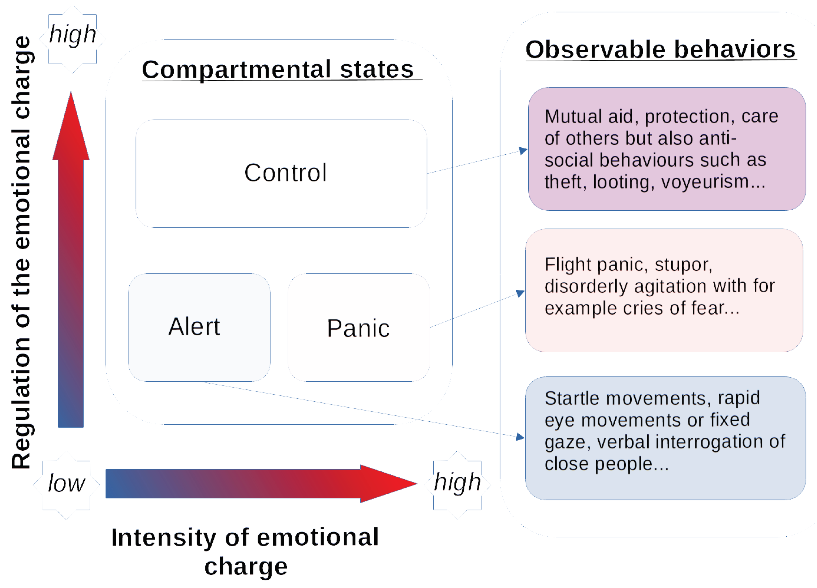
2.1. Emotional Load and Its Regulation

Within the framework of the Com2SiCa project, we focused on two key variables to identify and characterize different human behaviors occurring during a sudden catastrophe: the intensity of the emotional charge and its regulation. The first corresponds to the quantitative aspect of the emotion, and is adaptive to situations of threat or catastrophe [20]. We note that the intensity of the emotion is high in situations of fear or stress. The second is defined as the processes involved in adapting to relatively strong emotional episodes. Most researchers agree that emotions are not uncontrollable forces but they can be modulated when necessary (see [21] and the references within). Furthermore, adaptive emotion regulation consists in modulating—not eliminating—the experience of emotions [22,23]. By crossing these two variables, we characterized a wider range of human behaviors that may occur during a disaster than the sole panic behavior. As this behavioral diversity is difficult to model mathematically, we reduced it by identifying the behavioral states in which reactions can be located. Hence, three behavioral states were proposed:
  • The alert state corresponds to a low emotional charge and low regulation. It relates to a phase of assimilation of information relative to the event, a moment when people search in a very short time for information about the scenario they are experiencing. It marks a break from everyday behavior. Alert behaviors are often described by startle movements, rapid eye movements or a fixed gaze, and verbal interrogation of people close by;
  • The controlled state corresponds to an emotional charge which is more or less strong. This emotional charge is regulated which is why this behavior is controlled. People can regulate their emotions, to act and adapt their behavior to the crisis context. The controlled behavior does not ensure the safety of the person or the individual’s survival. It concerns behaviors such as mutual aid, protection and care of others but also anti-social behaviors, such as theft, looting, and voyeurism;
  • The panic state corresponds to a high emotional charge and a low regulation insufficient to provide a controlled behavior. Individuals in panic can adopt behaviors of panic flight, stupor, and disorderly agitation with cries of fear, for example.
Scientists in the humanities and social sciences can use different methods to differentiate these states. For example, they can associate each one with different physical manifestations that they can observe during a catastrophic event (Figure 1). They can collect physiological data to capture these behaviors and quantify them. Alert and control behaviors are associated with basic physiological states such as a low heart rate contrary to panic states. To capture these three states by simulation in a virtual reality experiment, physiological measures may be used, such as electrocardiograms and skin conductance. The aim is to quantify the emotional load and its intensity from the perspective of learned or controlled behaviors versus instinctive or automatic ones (see Section 3).
Since people do not maintain the same behaviors all the time, psychologists define two types of transitions between these three states. The first are the natural transitions specific to individuals depending on their experiences and their past. The second is imitation or social comparison which is important factor in the process of behavioral change [24]. Depending on a certain predisposition, the perception of the behavior of others encourages people to act in the same way [25]. In these collective circumstances and faced with an uncertain situation, that is to say, the absence of clear benchmarks for action, people can set up a mechanism of social comparison leading them to trust others and to consider the behavior of others as a reference and an example to follow. This form of informational imitation reduces the feeling of uncertainty.

2.2. Modeling the Dynamics of Human Behavior: Cross-References between the Social and Mathematical Sciences

The modeling of these different behaviors and their dynamics is presented below and is inspired by classical epidemic models, the Susceptible-Infected-Recovered (SIR) models [26]. As for SIR models, the population in situation of catastrophe is subdivided in several categories according to the adopted behavior and their different interactions are considered.

2.2.1. Structural Components of the APC Model

The mathematical Alert-Panic-Control (APC) model aims to describe the different behaviors during a catastrophic event, their temporal dynamics, i.e., the transitions from one state to another, and the responses to them due to qualitative parameters, i.e., the environmental context or group effects.
A catastrophic event marks a transition from everyday behavior to reactions specific to the disaster. That is why we consider a population of size N with an everyday behavior. We denote by A, C, and P, the population in the alert, the control and the panic states, respectively, and Q and B those exhibiting an everyday behavior. The first (Q) can be observed before the event starts but the second (B) occurs during or after the event. We suppose that the beginning of the catastrophe (resp. the end of the catastrophe) is modeled by the function γ (resp. φ ). Thus, when the catastrophe is triggered at time t ( γ ( t ) 0 ), a proportion γ ( t ) Q ( t ) of people with an everyday behavior become aware of an imminent danger and adopt an alert behavior, seeking information about what happened. Then, depending on intrinsic and imitation processes, as explained above, people in alert state adopt either a control or a panic behavior. Finally, after a certain time, people in a control state begin to return to everyday life, by seeking shelter for example, at a proportion φ ( t ) C ( t ) at time t.
Concerning the transitions (Figure 2), the parameters represented in blue, B i , i = 1 , , 4 , and C i , i = 1 , 2 designate the natural transitions specific to population based on their experience and past history. For B 3 and B 4 , the humanities and social sciences consider that populations engaged in a panic or control behavior can return to an alert state even if the probability is low. The second type of transition, F, G and H in the diagram, describes the imitation or social comparison processes as explained in the following section.

2.2.2. Imitation Processes

Imitation processes are important transitions in threat situations. Individuals can mimic the behavior either of another individual or of individuals within a small group by observation and perception of the behavior of the other or others. In the APC model, the imitation transitions are modeled as process contamination terms in SIR models. For example, the imitation process of control behaviors by individuals in alert is given by the term F ( A ( t ) , C ( t ) ) C ( t ) N A ( t ) . It models the probability for each individual with a control behavior to spread this behavior among individuals in alert and it is proportional to the portion of C in the whole population N = Q ( 0 ) + A ( 0 ) + C ( 0 ) + P ( 0 ) + B ( 0 ) . To express that the behavior of the majority influences the behavior of the minority through the process of imitation, we consider the following form for F:
F ( A , C ) = α η C A + ε ,
where ε < < 1 , 0 α 1 and η ( s ) = s 2 1 + s 2 is given in Figure 3. Since the value of the function η depends on the proportion of people in alert and control, the probability varies according to the proportion of control and alert individuals. The function η models that the higher the number of people with a control behavior, the higher the number of people with an alert behavior who will imitate those with a control behavior.
Analogously:
G ( A , P ) = β η P A + ε H ( C , P ) = γ p c η C P + ε γ c p η P C + ε
where β , γ p c , γ c p [ 0 ; 1 ] .
For the imitation term H, the imitation can go from panic to control and from control to panic.
Note that the imitation process can go in both directions between control and panic but not between alert/control and alert/panic, according to psychologists, since alert is a state that passes too rapidly to be imitated.

2.2.3. The Complete Model

The APC model comprises 5 equations, each one describing the evolution in time (in seconds in this article) of one of the population groups. Following Figure 2, the APC mathematical model is the following:
d A ( t ) d t = γ ( t ) Q ( t ) ( B 1 + B 2 ) A ( t ) + B 3 C ( t ) + B 4 P ( t ) F ( A ( t ) , C ( t ) ) C ( t ) N A ( t ) G ( A ( t ) , P ( t ) ) P ( t ) N A ( t ) , d C ( t ) d t = B 1 A ( t ) + C 1 P ( t ) ( B 3 + C 2 ) C ( t ) + F ( A ( t ) , C ( t ) ) C ( t ) N A ( t ) + H ( C ( t ) , P ( t ) ) P ( t ) N C ( t ) φ ( t ) C ( t ) , d P ( t ) d t = B 2 A ( t ) + C 2 C ( t ) ( B 4 + C 1 ) P ( t ) + G ( A ( t ) , P ( t ) ) P ( t ) N A ( t ) H ( C ( t ) , P ( t ) ) C ( t ) N P ( t ) , d Q ( t ) d t = γ ( t ) Q ( t ) , d B ( t ) d t = φ ( t ) C ( t ) .
Model (3) is rewritten in terms of fraction of the population instead of numbers of individuals:
d a ( t ) d t = γ ( t ) q ( t ) ( B 1 + B 2 ) a ( t ) + B 3 c ( t ) + B 4 p ( t ) F ˜ ( a ( t ) , c ( t ) ) c ( t ) a ( t ) G ˜ ( a ( t ) , p ( t ) ) p ( t ) a ( t ) , d c ( t ) d t = B 1 a ( t ) + C 1 p ( t ) ( B 3 + C 2 ) c ( t ) + F ˜ ( a ( t ) , c ( t ) ) c ( t ) a ( t ) + H ˜ ( c ( t ) , p ( t ) ) p ( t ) c ( t ) φ ( t ) c ( t ) , d p ( t ) d t = B 2 a ( t ) + C 2 c ( t ) ( B 4 + C 1 ) p ( t ) + G ˜ ( a ( t ) , p ( t ) ) p ( t ) a ( t ) H ˜ ( c ( t ) , p ( t ) ) c ( t ) p ( t ) , d q ( t ) d t = γ ( t ) q ( t ) , d b ( t ) d t = φ ( t ) c ( t )
with ( ε ˜ = ε N )
F ˜ ( a , c ) = α η c a + ε ˜ , G ˜ ( a , p ) = β η p a + ε ˜ , H ˜ ( c , p ) = γ p c η c p + ε ˜ γ c p η p c + ε ˜ .
It can be rewritten:
x ˙ ( t , θ ) = ψ ( t , x , u , θ )
where x = ( a , c , p , q , b ) T = ( A / N , C / N , P / N , Q / N , B / N ) T [ 0 , 1 ] 5 , u = ( γ , φ ) , θ = ( B 1 , B 2 , B 3 , B 4 , C 1 , C 2 , α , β , γ c p , γ p c ) D with D : = ( R + ) 6 × ( R + ) 4 .
At the initial time, the entire population is supposed to be engaged in an everyday behavior so that the following initial conditions are considered:
x ( 0 ) = ( 0 , 0 , 0 , 1 , 0 ) T .
Following the proof of [2], the proposition is deduced:
Proposition 1.
The Cauchy problem (6)–(7) admits a unique maximal non-negative solution for any value of the parameters θ D .

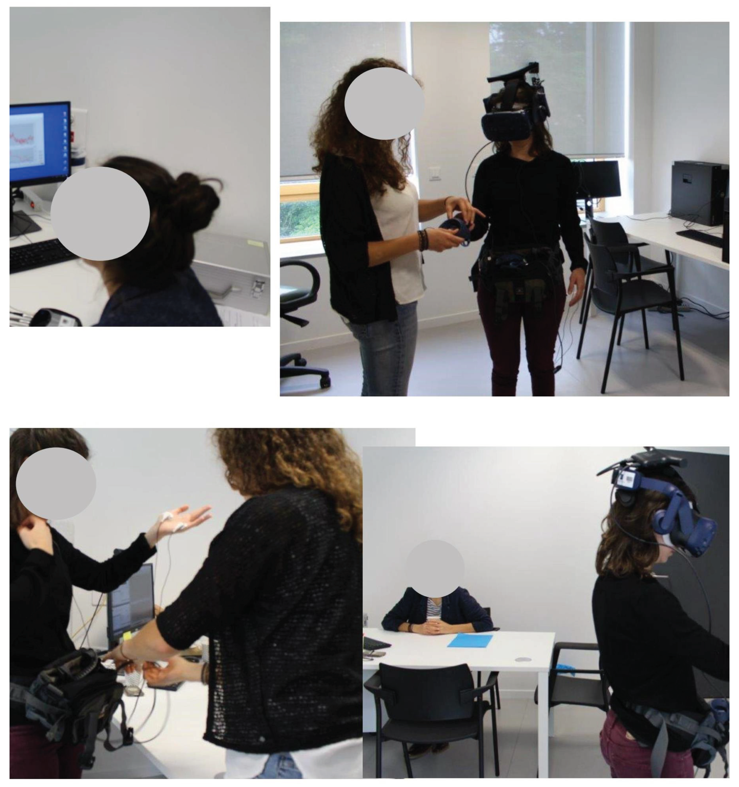
3. The Virtual Reality (VR) Experiment

The VR experiment was conducted by psychologists in the LPPL laboratory of Nantes (France) in a closed and controlled environment. Its aim was to determine from physiological measurements, the different behavioral states and the changes occurring during a catastrophic event by taking into account the environmental context, such as the type of event, the spatial configuration, and the presence or absence of individuals.

3.1. The VR Experimental Procedure and Sample

This VR experiment consisted in immersing individuals in the simulation of a tsunami on the Mediterranean coast of Nice (France), a scenario event which has since been included in national regulatory tools. The scenario of the simulation was based on research data (See [27]). To construct the spatial context, topographical information was gathered in Nice regarding the beach, such as its width, the presence of stairs, pebbles, and access guardrails, etc. (See [28]). Virtual characters (avatars) were also included to observe behavioral reactions in the context of social interactions between the survey respondents and the avatars.
Three scenarios were built based on three experimental conditions, designed to simulate different reactions, to compare them and to better understand how the context affects behavior. For example, a situation of danger does not automatically generate a feeling of threat if the person is alone. The reaction depends on the person’s experience and the behaviors of those around whose behavior can be imitated. The three following scenarios were carried out:
  • First scenario (neutral scenario): in this experimental condition, the person is alone without any virtual person;
  • Second scenario (organized scenario): in this experimental condition, the person is in the presence of virtual persons with a suitable behavior (escape from the tsunami by walking quickly in the right direction and without shouting);
  • Third scenario (non-organized scenario): in this experimental condition, the person is in the presence of virtual persons with an unsuitable behavior (escape by running in all directions and shouting).
In the second scenario, the physical reactions of the avatars express a control behavior whereas in the third one they express panic.
Eighty-eight unpaid volunteers were recruited through the local press and were assigned randomly to one of the three conditions. The sample was composed of 43 women and 45 men. Their age ranged from 18 to 56 years with a mean of 26.76 years and a standard deviation of 9.41. The participants were divided into the different conditions by respecting a balance between men and women, and a diversity in the ages. Therefore, 29 persons were assigned to the first and third scenario and 30 to the second one. The distribution of the participants with respect to their sex and the scenario is provided in Table 1.
During the simulation, each participant was immersed in a virtual reality environment that provides a visual and auditory feedback (Figure 4). The subject was directly placed on the beach at the beginning of the simulation and had free movements. To capture and maintain the participant’s attention, the proposed timeline was based on how a tsunami on the Mediterranean coast of Nice is perceived rather than the reality of its dynamics. As decided, after 60 s, the level of the sea decreased. Then, the wave formed on the horizon, and the water noises became louder. The wave reached the beach after 3 min. If the participants stayed immobile on the beach, the application stopped when they were struck by the wave. If the participants had an escape behavior inside the city, the application stopped when they reached a city exit. In all other cases, the application stopped 2 min after the wave submerged the beach. The steps are summed up in Figure 5.
All subjects gave their informed consent for inclusion before they participated in the study. The study was conducted in accordance with the Declaration of Helsinki, and the protocol was approved by the Ethics Committee of University of Angers, France (CER_20200114).

3.2. Measurements

Physiological measurements were recorded for each participant to determine their emotional charge at each moment of the simulation. A Nexus X MKII device was connected to the participant by electrodes. It recorded for each of them an electrocardiogram (ECG) and skin conductance in order to identify any stress signals when faced with the tsunami. The ECG is a recording that provides different variables relevant for detecting of a state of stress [29]. It reports successive polarization and depolarization of the heart, translated into the characteristic peaks of this type of recording. In particular, it provides the Heart Rate (HR) expressed as beats per minute, calculated from the frequency of apparition of a type of peak during one minute of recording. Skin conductance measures the continuous variation in the electrical characteristics of the skin. The data are collected by applying a low, undetectable, and constant voltage to the skin and then measuring how the skin conductance varies.
In our study, only the ECG and more specifically the HR, were retained because of their reliability [30]. Even if the experiment was conducted in a laboratory, the slight movements of the participants distorted some of the conductance measurements.
Before starting each simulation, the experimenters carried out a test to check that the devices functioned properly (VR and physiological measurements) and to familiarize the participants with VR. Thus, all participants experienced the same test situation, which was an immersion in a Viking village. This test also allowed us to record a base line of the HR at rest specific to each individual. Throughout the VR experiment, the stress state of each participant was determined in comparison with the base line: a state of stress was identified as soon as the participant’s HR exceeded the base line and, therefore, increased.
From the HR measurements, two categories of persons were distinguished: calm and stressful persons corresponding to a low HR and a high HR, respectively. Consequently, two series of measurements were obtained.
In the following section, we show the links between the physiological measurements and the corresponding variables of the model.

4. The Link between the Mathematical Model and the Experimental Data

According to [31] and Section 2, three types of behavioral states occur during a catastrophic event with respect to their emotional charge and the capacity of individuals to regulate it: the alert, control and panic states. In the following section, we associate these states with the psychological measurements.

4.1. Observed Variables of the Mathematical Model

In this section, we determine which variables or combinations (of variables) of the mathematical model can be associated with one of the experiment measures.
Based on knowledge in psychology and physiology, alert and control behaviors correspond to a basic state in which persons have a low heart rate (HR) contrary to the panic behavior (see Section 2 and [30]). During the VR experiments, two sets of measurements distinguished from the cardiac measurements were associated with a low HR or a high HR. Therefore, we consider that the first set of measurements correspond to everyday, alert and control behaviors in the APC model and the second set to the panic behavior. Persons returning to everyday life in the mathematical model can be identified by persons moving to safety in le vieux Nice or finishing the simulation. Their percentage during the experiment time corresponds to the difference between the total number of survey respondents and the number of control and panic respondents.
The data provided by the psychologists are gathered in Table 2 and represent the percentages of survey respondents exhibiting daily-alert-control behavior, panic behavior and return to everyday behavior in the three scenarios (neutral, organized, and non-organized). A graphical representation of the distribution of these behavioral states over time is provided in Figure 6 for the neutral scenario.
The next step was to convert the data in Table 2 into densities for the mathematical treatment. We denote S m as the density of persons with a low HR corresponding to the first set of measurements, p m the density of persons with a high HR corresponding to the second set and b m : = 1 S m p m the density of persons who finished the VR scenario.
The corresponding variables of the mathematical model (4) are denoted y 1 = q + a + c , y 2 = p and y 3 = b . They are also called outputs of the model. The aim of the following step was to search for the best parameters to make the trajectories of the model fit as closely as possible to the experimental data such as those of Figure 6 for the neutral scenario.

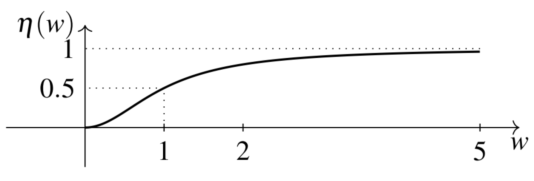
4.2. Modeling the Beginning and the End of the Catastrophe

From Figure 5 and Table 2, a simple representation of functions γ and φ can be found. In the scenario of the VR experiment, the survey respondents are supposed to be engaged in an everyday behavior until the 60 s point, the moment at which the beginning of the wave can be heard. Thus, γ that models the catastrophe is supposed to be equal to 0 up to 60 s. Then, at 90 s, when the siren sounds, we suppose that all the persons become aware of the imminent arrival of danger. Consequently, 100% of survey respondents have adopted in one of the three behaviors: alert, control or panic behavior. Between 60 and 90 s, we assume that the percentage of people aware that a disaster is regularly increasing. Using the function
ϕ ( s ) = 0 if s < τ 0 1 if s > τ 1 1 2 1 2 cos s a b a π if τ 0 s τ 1
an approximation of γ with τ 0 = 60 , τ 1 = 90 is obtained (see Figure 7).
In the same way, the function φ describing the return to an everyday behavior is constructed from ϕ with τ 0 (resp. τ 1 ) as the time at which the first survey respondent (resp. the last one) left the simulation. φ must be calculated for each scenario since persons do not adopt the same behaviors. For example, the organized scenario ends at 280 s contrary to the non-organized scenario that ends at 200 s. This difference shows that imitation processes were different depending on the scenario.

5. Identifiability and Minimal Number of Observation Data

This section describes the strategy implemented to estimate the parameters from the set of measurements provided in Table 2. Two strategies are possible. The first is to follow the three VR scenarios and estimate first the intrinsic parameters and then, from their knowledge, estimate the imitation processes in the organized and non-organized scenario. A second possible strategy is to estimate all the parameters from the two scenarios integrating imitation processes (organized and non-organized scenarios) without any knowledge of the intrinsic parameters.
To determine the best strategy, a global identifiability study is first carried out on the Model (6) to which the model outputs are added. The global identifiability of the model makes it possible to determine whether without noisy data and with sufficient data, all the parameters or groups of parameters can be uniquely characterized from the model outputs in all the search domain. A further specific study serves to determine whether the number of measurements is sufficient to estimate all or groups of parameters. This mathematical study will show that the second strategy does not allow us to estimate all the parameters from the second and third scenarios due to a lack of measurements as opposed to the first strategy. Therefore, the strategy selected has to correspond to VR protocol which is to first estimate the intrinsic parameters and then the imitation processes.
For the mathematical studies, we add the outputs to Equation (6) and set:
x ˙ ( t , θ ) = ψ ( t , x ( t , θ ) , u ( t ) , θ ) , y ( t , θ ) = h ( x ( t , θ ) , θ ) R 3 .

5.1. Identifiability

5.1.1. Definition

The identifiability property ensures that two different parameter vectors generate two distinct trajectories. More precisely:
Definition 1.
Let P be an admissible set of parameters. The model (9) is said to be globally identifiable at θ if a time t 1 [ 0 , T ] exists such that for all t [ 0 , t 1 ] , for all θ ¯ P , θ ¯ θ , the trajectories y ( t , θ ) and y ( t , θ ¯ ) are different.

5.1.2. Method

To test the identifiability of the model, the method proposed in [32] and performed in [33] is also used. It is based on differential polynomials that is, expressions constructed from variables t, x, u, y, parameters θ i and constants. Specific output-polynomials depending only on the model outputs y, the inputs u, and the parameters θ i are obtained with the Rosenfeld–Groebner algorithm, an elimination algorithm. From the specific order [ y , u ] [ x ] that consists in eliminating the unknown state variables (here the block [ v ] means that v and its derivatives are ordered by the ranking < such that v < v ˙ < v ¨ < and ≺ indicates a block elimination ranking in the sense “ranks lower than” between two blocks), it triangulates the differential equation system (9) using the operations of addition, subtraction, multiplication and derivation. A general set of differential polynomials with pairwise distinct leading derivatives is obtained and its solutions are the general solutions of (9) and reciprocally. The specific output-polynomials belong to this set. They can be rewritten in the following form (see [32]):
P i ( y , u , θ ) = m 0 i ( y , u ) + j = 1 q i Θ j i ( θ ) m j , i ( y , u ) = 0 , i from 1 to 3
where ( Θ j i ) 1 j q i are rational in θ , Θ v i Θ w i ( v w ), ( m j , i ) 1 j q i are differential polynomials with respect to y, m 0 i 0 . The highest ranking derivative which appears in P i is called the leader. For example, with the elimination order [ x 1 ] [ x 2 ] , the leader of the differential polynomial p ( x 1 , x 2 ) = x 1 2 + x ˙ 2 + x 2 + x 1 x ¨ 2 is x ¨ 2 .
According to [32], the algorithm returns as many output-polynomials as outputs. In our case, we have 3 output-polynomials, and the leader of the polynomial in P i corresponds to y i .
From then onwards, to simplify the notations, only one output is considered such that the index i is omitted. Let us denote by s the highest time derivative order of y in P.
From the coefficients of the polynomial P, the initial conditions, if any, and the constraints on the parameters, we can define the real-valued function ϕ by
ϕ : θ = ( θ 1 , , θ p ) P ( Θ 1 , , Θ q , y ( 0 , θ ) , , y ( s 1 ) ( 0 , θ ) )
where P is an a priori known admissible set of parameters. Under some technical conditions omitted in this paper (for more details, the interested reader can refer to [32]), the identifiability result is the following:
Proposition 2.
We assume that the Wronskian W ( m 1 , , m q ) = det ( m k ( y , u ) , k = 1 , , q ) is not identically equal to zero (To verify this assumption, it is sufficient to verify the linear independence of the m k ( y , u ) , k = 1 , , q . In fact, the monomials are linearly independent if there exists a time point at which the Wronskian is non-zero.).The model (9) is globally identifiable if the function ϕ is injective on P .
Remark 1.
To test the identifiability of the APC model, we used the IdentifiabilityTree algorithm developed in [33] and implemented in Maple. This algorithm provides the set of key parameters leading to the identifiability of the model and can ultimately test its global identifiability. The first step is to use the Rosenfeld–Groebner algorithm to obtain the output-polynomials. From the coefficients of these differential polynomials, the second step uses IdentifiabilityTree algorithm. This algorithm tests the identifiability of a given parameter when some parameters are known. The reason is that, in some applications, the identifiability property of the mathematical model may depend on the knowledge of some key parameters. The algorithm returns a set of parameter lists, and each set gives the identifiability of one parameter with respect to the others. In practical terms, if a parameter θ l is not identifiable, the lists gives the parameters that has to be identified to obtain the identifiability of θ l . If the model is identifiable, only one list containing all the parameters of the model is returned.
At the end of this step, we have the following assumptions H :
  • Functions of γ and φ are known;
  • y 1 ( t ) = q ( t ) + a ( t ) + c ( t ) , y 2 ( t ) = p ( t ) , y 3 ( t ) = b ( t ) .

5.1.3. Identifiability of the APC Model with No Imitation

In this section, we consider the first scenario where there is no imitation. The consequences for the mathematical model are that F = G = H = 0 and the parameter vector that we want to identify is θ ˜ : = ( B 1 , B 2 , B 3 , B 4 , C 1 , C 2 ) .
Remark 2.
The identifiability of the model at θ ˜ when F = G = H = 0 means that the intrinsic parameters could be estimated uniquely from the first scenario with perfect, noisy-free data. Assuming that the profile of participants is the same in the three scenarios and, therefore, also the intrinsic parameters, the imitation parameters can be estimated from the second and third scenarios if they are identifiable.
The following proposition gives the identifiability result when α = β = γ 1 = γ 2 = 0 , and rewritten in an equivalent way F = G = H = 0 .
Proposition 1.
If there is no imitation, under the assumption H , model (9) is identifiable with respect to θ ˜ .
Proof of Proposition 1.
The IdentifiabilityTree algorithm is applied with the elimination order [ y 1 , y 2 , y 3 ] [ q , a , c , p , b ] .
The output-polynomials given by the Rosenfeld–Groebner algorithm are:
P 1 : = ( B 1 B 2 C 2 + B 1 C 2 2 B 2 2 B 3 B 2 2 C 2 + B 2 B 3 C 2 + B 2 C 2 2 ) y ˙ 3 + B 2 C 2 y ˙ 3 φ + B 2 ( y ¨ 2 + y ˙ 2 γ ) φ + ( B 2 2 B 2 C 2 ) y ˙ 3 γ + ( B 1 B 2 B 1 C 2 + B 2 2 + B 2 B 4 + B 2 C 1 ) y ˙ 2 φ + ( B 1 B 2 B 4 + B 1 B 2 C 1 B 1 B 4 C 2 B 1 C 1 C 2 + B 2 2 C 1 B 2 C 1 C 2 ) y 2 φ + ( B 2 B 4 + B 2 C 1 ) y 2 γ φ B 2 2 y 1 γ φ = 0 , P 2 : = B 2 ( y ˙ 3 φ ˙ + y ¨ 3 φ + y ˙ 3 φ 2 ) + ( B 1 C 2 + B 2 B 3 + B 2 C 2 ) y ˙ 3 φ B 1 y ˙ 2 φ 2 + ( B 1 B 4 B 1 C 1 B 2 C 1 ) y 2 φ 2 = 0 , P 3 : = y ˙ 1 + y ˙ 2 + y ˙ 3 = 0
The third polynomial is not informative on the coefficients, thus only P 1 and P 2 will be used to study the identifiability of the model. To put these polynomials in the form (10), we let B ˜ 1 : = B 1 B 2 ( B 2 is supposed to be non-zero) and we divide P 1 and P 2 by B 2 . The following real-valued function is obtained ϕ ( θ ) = ( B 2 , C 2 , B 2 C 2 , B 4 + C 1 , ( B 2 C 2 ) B ˜ 1 + B 2 + B 4 + C 1 , ( B 2 C 2 ) ( B ˜ 1 C 2 + B 3 + C 2 ) , ( ( B 4 + C 1 ) B ˜ 1 + C 1 ) ( B 2 C 2 ) , B ˜ 1 , B ˜ 1 C 2 + B 3 + C 2 , ( B 4 + C 1 ) B ˜ 1 + C 1 ) .
Under the set of conditions C ( θ ) = { B ˜ 1 > 0 , B 2 > 0 , B 3 > 0 , B 4 > 0 , C 1 > 0 , C 2 > 0 } , the algorithm IdentifiabilityTree allows us to conclude that the parameters B ˜ 1 , B 2 , B 3 , B 4 , C 1 , C 2 are identifiable, and consequently B 1 too. □

5.1.4. Identifiability of the Imitation Parameters

Now that the parameters of the linear part are known, an identifiability study can be carried out on the set of imitation parameters that is θ ˇ : = ( α , β , γ c p , γ p c ) . We have the following proposition.
Proposition 3.
We assume that the intrinsic parameters are known. Under the assumption H , the model (9) is identifiable with respect to the θ ˇ .
Proof. 
First, according to the last equation of (4), c can be supposed as an output of the model since b and φ are known according to assumption H . Let y 4 : = c . The sum of the first three equations of (4) is equal to:
a ˙ + c ˙ + p ˙ + q ˙ = γ q φ c .
Equation (13) can also be rewritten q ˙ + γ q = y ˙ 1 + y ˙ 2 φ y 4 . This differential equation has a unique solution with the initial condition q ( 0 ) = 1 . Furthermore, q can also be considered too as an output of the model. Let y 5 : = q . Finally, from (13), we deduce that y 6 : = a is an output of the model. Consequently, the first three equations of (9) are output-polynomials.
To prove the identifiability of the imitation parameters α and β , it is sufficient to prove that the functions φ 1 ( t ) = c ( t ) 3 ( a ( t ) + ε ˜ ) 2 + c ( t ) 2 , φ 2 ( t ) = p ( t ) 3 ( a ( t ) + ε ˜ ) 2 + p ( t ) 2 are linearly independent. To test this condition, we evaluate the Wronskian
W ( φ 1 , φ 2 ) = φ 1 ( t ) φ 2 ( t ) φ ˙ 1 ( t ) φ ˙ 2 ( t )
that gives
W ( φ 1 , φ 2 ) = 3 p ( t ) 2 c ( t ) 2 A + B 2 C 3 D e n
with
A : = ( ( a ( t ) + ε ˜ ) 2 + p ( t ) 2 ) p ( t ) ( c ( t ) 2 3 + ( a ( t ) + ε ˜ ) 2 ) c ˙ ( t ) , B : = c ( t ) ( p ( t ) 2 / 3 + ( a ( t ) + ε ˜ ) 2 ) ( ( a ( t ) + ε ˜ ) 2 + c ( t ) 2 ) p ˙ ( t ) , C : = a ˙ ( t ) p ( t ) c ( t ) ( c ( t ) p ( t ) ) ( c ( t ) + p ( t ) ) ( a ( t ) + ε ˜ ) D e n : = ( c ( t ) 2 + a ( t ) 2 + 2 a ( t ) ε ˜ + ε ˜ 2 ) ( a ( t ) 2 + 2 a ( t ) ε ˜ + p ( t ) 2 + ε ˜ 2 ) 0 .
The Wronskian is not identically equal to zero. Therefore, α and β are identifiable. We can prove in the same manner that γ p c and γ c p are identifiable. □
Remark 3.
To prove the identifiability of the APC model with no imitation (see Section 5.1.3) we could use the same reasoning as in the previous proof. However, we need an explicit expression of the output-polynomials to determine the minimal number of measurements in Section 5.2.

5.1.5. Identifiability of the Complete Model

The following proposition gives the identifiability result of the complete model.
Proposition 4.
Under assumption H , model (9) is identifiable.
Proof. 
Using the same arguments as in the proof of Proposition 3, we find that the equations of the model are output-polynomials and that all the parameters are identifiable. □
Remark 4.
The output-polynomials deduced from the complete model (with imitation terms) and the Rosenfeld–Groebner algorithm have a higher time derivative order than P 1 and P 2 defined at (12). Because of the non-linear terms corresponding to the imitation processes, more derivation operations are necessary in the elimination procedure to obtain the corresponding output-polynomials.

5.2. Minimal Number of Observation Data

In [34,35], the authors proposed a method to determine the minimal number of observation points in order to obtain the local identifiability of the system. The result is based on the generation of a function ρ = ρ ( Θ , y , y ˙ , , y ( k ) ) , where k is a non-negative integer, such that ρ has continuous partial derivatives with respect to Θ . The local identifiability results from the local inversion of ρ by using the implicit function theorem in a neighborhood where the function vanishes. [34] noticed that differential polynomials obtained from differential algebra methods can generate this function ρ . We present below an adaptation of their result with the output-polynomial (10).
To simplify the notations in this section, we consider only one output-polynomial. The index i is, therefore, omitted in (10). We denote the coefficients of P by Θ = ( Θ k ( θ ) ) k = 1 , , q . Note that P 1 and P 2 defined at (12) can be rewritten in this form.
Proposition 5.
Let us assume that
1. 
The function
ρ : R q × R m R q ( Θ , y ) ( P ( θ , y ) , P ( θ , y ) ( 1 ) , , P ( θ , y ) ( q 1 ) )
is a differentiable function with respect to the first variable;
2. 
The function ϕ defined at Equation (11) is injective;
3. 
The Wronskian W ( m 1 , , m q ) defined at Proposition 2 is not identically equal to zero.
In order to have the local identifiability of the model, the minimum number of measurements of y is s y + q , where s y is the higher order derivative of y in P.
Proof. 
First, note that by definition ρ vanishes for all y and Θ . Then, let us apply the Taylor expansion of ρ at Θ *
ρ ( Θ , y ) ρ ( Θ * , y ) + ( Θ Θ * ) ρ Θ ( Θ * , y ) .
By definition, ρ ( Θ * , y ) = 0 and ρ has continuous partial derivatives with respect to Θ , thus
ρ Θ = P Θ 1 P Θ q P ( q 1 ) Θ 1 P ( q 1 ) Θ q = m 1 m q m 1 ( q 1 ) m q ( q 1 ) .
By assumption, ρ Θ is the Wronskian W ( m 1 , , m q ) which is supposed to not be identically equal to zero. According to (17), Θ can be expressed as a differentiable function of y and its derivatives up to its s y + q 1 order derivative. Or to evaluate a derivative of order s y + q 1 , s y + q points are needed. Consequently, to have the local identifiability of the model, the number of measurements of y must be at least s y + q . □
Remark 5.
In the case where Assumption 2. is difficult to check, i.e., the functional determinant ρ Θ is difficult to calculate because it may require high formal calculus, it can be replaced by the following:
q distinct time points t 1 , , t q exist such that the determinant
P Θ 1 ( t 1 ) P Θ q ( t 1 ) P Θ 1 ( t q ) P Θ q ( t q )
is not identically equal to zero.
Example 1.
Consider the output-polynomials P 1 and P 2 given in (12). They are needed to identify all the parameters. After dividing P 1 by B 2 , we obtain a polynomial of the form (10) composed of 7 coefficients and whose indeterminates are y 1 , y 2 , y 3 . Its leader is y ¨ 2 . This polynomial must be derived six times to get a square system. The higher order derivative in P 1 is 2 for y 2 and 1 for y 3 . Consequently, the higher order derivatives of the system composed of 7 equations are 8 for y 2 and 7 for y 1 . To evaluate a derivative of order 8 (resp. order 7), 9 points are needed (resp. 8 points). Finally, 9 measurements are needed to estimate the coefficients of the output-polynomial P 1 / B 2 .
Using the same argument with P 2 / B 2 , we deduce that 3 + 2 = 5 measurements of y 3 (resp. 3 + 1 = 4 measurements of y 2 ) are needed to estimate its coefficients.
In conclusion, the minimal number of measurements required to have the local identifiability is 9.
Remark 6.
  • From the results of Section 3, we can conclude that a parameter estimation procedure can be implemented to estimate the intrinsic parameters using the data provided in Table 1. There is a unique parameter vector that allows the model outputs to fit the data of this table in the case of noisy-free measurements;
  • One could be tempted to estimate all the parameters of the model from the second and third scenario. However, from Remark 4, order derivatives of output-polynomials are higher and there are not enough measurement points to have the local identifiability.
In summary, the parameter identification will be carried out in three steps corresponding to the three conditions in the VR experiment. The main assumption is that the participants have the same profile in the three scenarios. For each one, a set of parameters will be estimated with respect to each scenario. The intrinsic parameters will be first estimated for the Neutral scenario in which there is no imitation process. Then, the parameters describing control imitation processes will be calculated from the organized scenario and the parameters describing the panic imitation processes from the non-organized scenario. Figure 8 summarizes the steps of identification.

6. Parameter Estimation

The parameter estimation procedure is accomplished following the steps defined in the previous section.

6.1. Minimization Problem
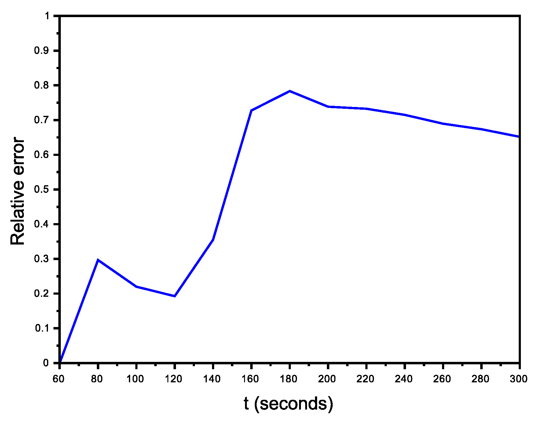
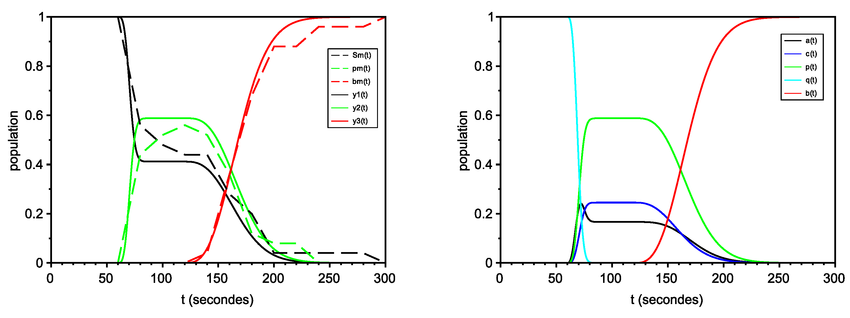
Given discrete-time measurements and a parametrized model describing a continuous-time process, we seek the parameter values best fitting the experimental data. To fulfill this objective, an optimization procedure is implemented to adjust the model parameters and the measurements. It is constructed from a L 2 cost function given by the sum of the square of the differences between the outputs of the model and the experimental data at each discrete time.
Let ( t i ) i = 1 , , M be the discrete time instants corresponding to the physiological measurements, S m , p m , and b m , defined in Section 4.1. These three vectors correspond to the densities of persons engaged in a control, panic and return to everyday behavior at each discrete time. Set y m e s = ( S m , p m , b m ) T and y ( θ ) = ( y 1 ( t i ) , y 2 ( t i ) , y 3 ( t i ) ) i = 1 , , M T obtained from the outputs of the model evaluated at each t i with the parameter vector θ , where the exponent “T” indicates the transpose of the matrix.
The cost function J ( θ ) is the square of the sum of the errors, that is
J ( θ ) = y m e s y ( θ ) 2 2 = i = 1 M j = 1 3 ( y i , j m e s y ( θ ) i , j ) 2
where y i , j m e s (resp. y ( θ ) i , j ) is the component at the i-th line and j-th column of the matrix y m e s (resp y ( θ ) ) and M is the number of discrete-time measurements.
The solution of the optimization algorithm is denoted
θ ^ = a r g m i n θ P J ( θ )
Several local and global optimization algorithms are proposed in the literature to solve this non-linear least-squares fitting [36,37]. The results of the optimization algorithms are the sets of parameters that produce the best fit between the simulations and experimental data.
In our case, local optimization algorithms such as Levenberg–Marquardt are not reliable for finding the global minimum since they require a first initial guess of the parameters that we do not have.
Global optimization methods and particularly stochastic ones such as simulated annealing, genetic algorithms, and evolutionary computation are suggested as the methods of choice when knowledge of the parameter values is lacking. Starting with a suitable initial domain, global optimization methods search more or less exhaustively through the parameter values in the attempt to minimize the cost function. One of the main problems associated with these methods is that they tend to be computationally expensive and may not perform well when the noise in the measurements is significant.
In this work, we chose the genetic algorithm inspired by Darwin’s theory of biological evolution [19,38]. This evolutionary algorithm imitates genetic processes. According to predefined operations, it generates children by selecting and combining/muting the best parents in the current generation. It reiterates this process until the population evolves into an optimal solution. Since it uses probabilistic transition rules instead of deterministic ones, it can search for solutions in a large domain. Furthermore, contrary to other algorithms, function derivatives are not required. For more details, the readers can refer to [39].
In the following section, we present the numerical results.

6.2. Results

The function optim_ga implemented in the software Scilab was used to estimate the parameters. The model outputs of the mathematical model are not very sensitive to the imitation parameters. We therefore just want to have an order of magnitude of these parameters.
To estimate the numerical errors in the parameters, the sum of the relative errors between the measurement curves and the model outputs with respect to time is drawn for each case.

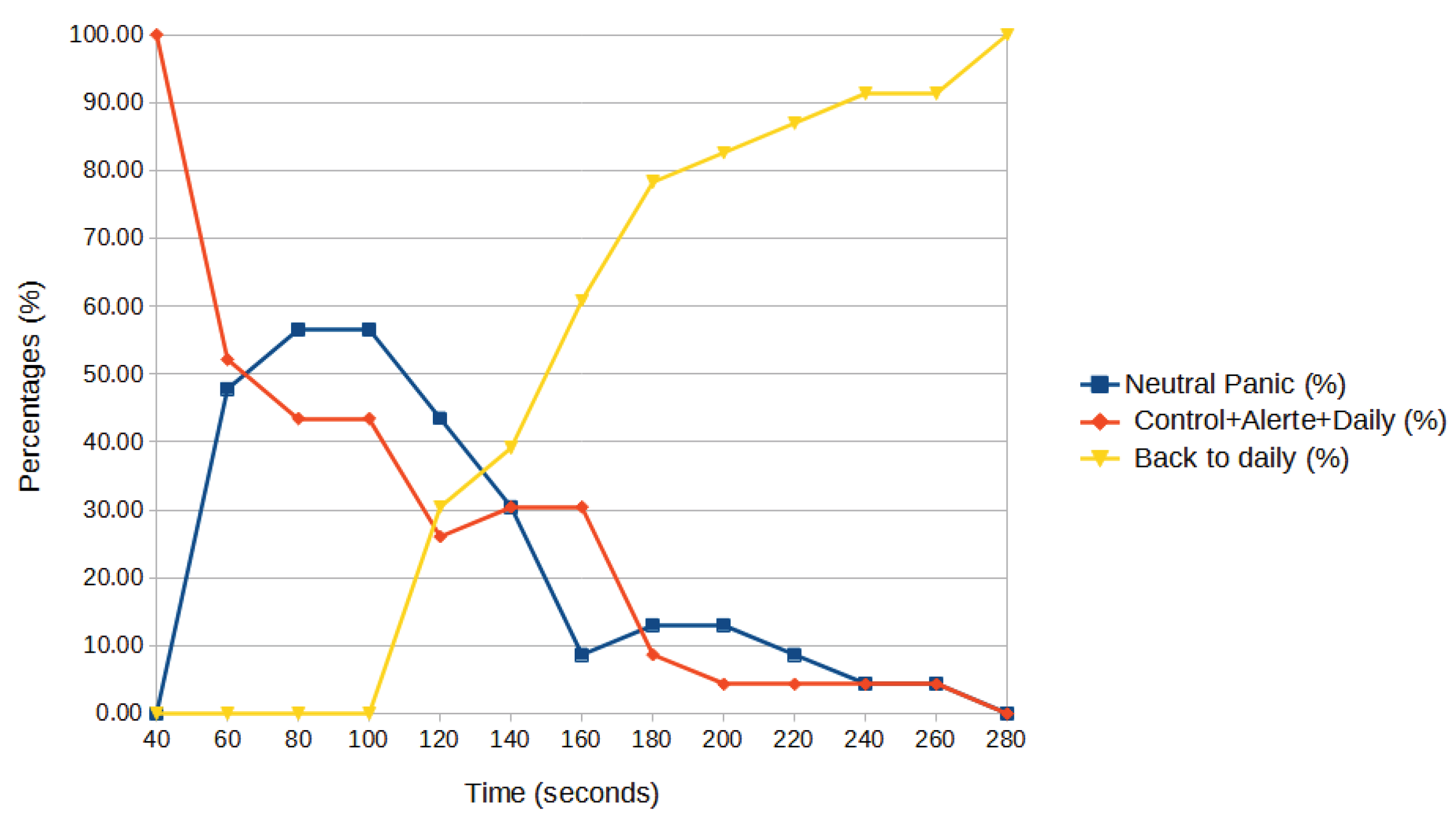
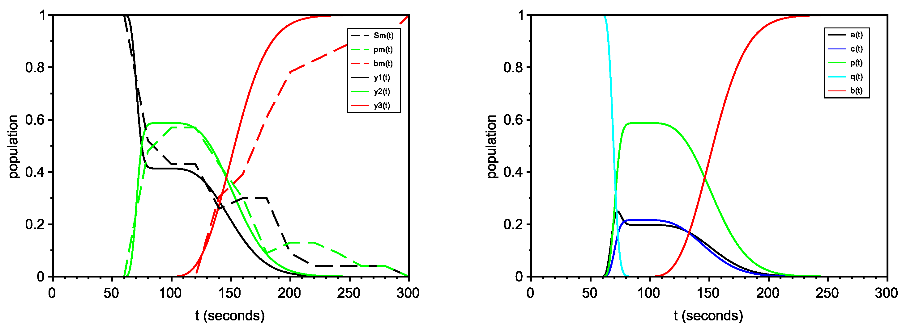
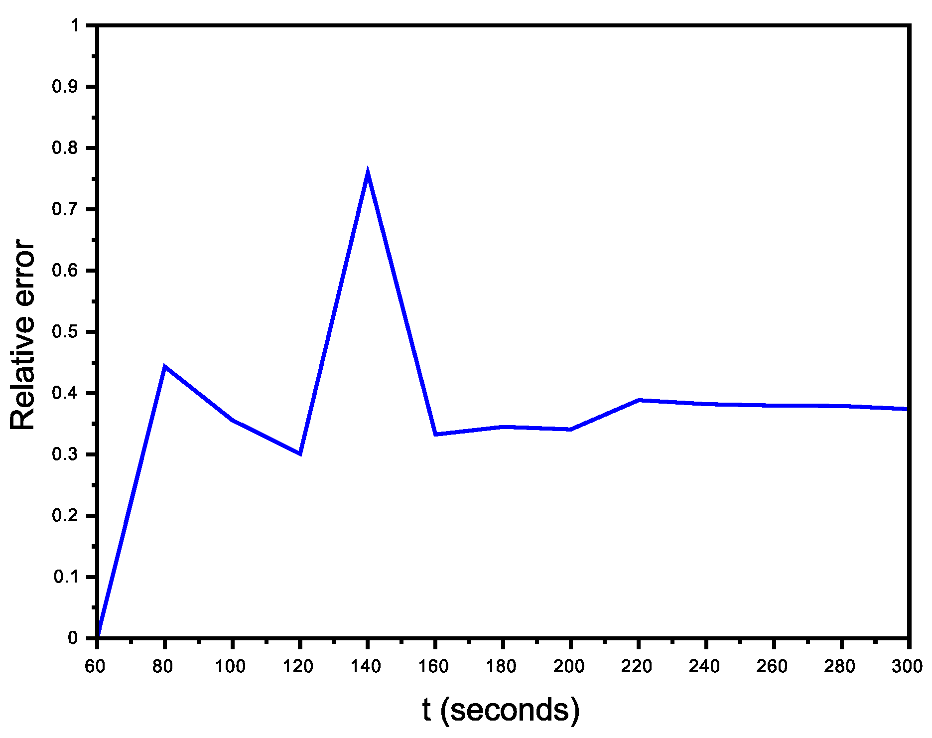
6.2.1. Scenario with No Avatars

In this scenario, 29 persons were surveyed but only 23 were kept because of the quality of their measurements. Indeed, either their signal was absent or it had too many artifacts due to little movements distorting the recorded measurements. In the optimization problem (21), the variables and their constraints are θ = ( B 1 , B 2 , B 3 , B 4 , C 1 , C 2 ) P where
P = { θ [ 0.01 , 0.7 ] 2 × [ 0.01 , 0.2 ] 2 × [ 0.01 , 0.7 ] 2 / B 2 + C 2 < 1 } .
Condition B 2 + C 2 < 1 was added to limit the panic behavior and make the algorithm convergent considering that the model is very sensitive to the intrinsic parameters and large values make the Runge–Kutta algorithm that solves system (4) divergent.
The genetic algorithm returns the following values for the intrinsic parameters: B 1 = 0.1915 , B 2 = 0.4374 , B 3 = 0.1009 , B 4 = 0.1741 , C 1 = 0.1448 , C 2 = 0.4676 .
The left subplot of Figure 9 represents the trajectories of the real data S m , p m , b m , and the trajectories of the outputs calculated with the estimated parameters. In the right subplot, the curves represent the simulations of a, p, c, b, q.
From the three output trajectories, the sum of the relative errors between the measurement curves is calculated and plotted with respect to time in Figure 10. The relative error increases between 120 and 150 s when individuals begin to move to safety in le vieux Nice but slightly decreases until the end of the scenario. Consequently, the mathematical model fits well with the beginning of the measurement curves. There is a slight degradation in the results when individuals begin to stop the VR but the relative error stays constant and decreases a little when considering a longer time.
Remark 7.
We note that the population has a low risk culture. The relations B 2 > B 1 and C 2 > C 1 imply that individuals tend to engage in a panic behavior on their own.

6.2.2. Organized Scenario

In the second scenario, 25 persons were selected again among 29. The values of the intrinsic parameters found in the first scenario were used. In this scenario, since there are no panic avatars, we assume that β = γ c p = 0 .
The optimization problem is solved with θ = ( α , γ p c ) and P = [ 0 , 9 ] 2 . The results obtained with the genetic algorithm are θ ^ = ( α , γ p c ) = ( 0.8338 , 0 ) . Figure 11 gives the representation of real data and the output trajectories evaluated with θ ^ and the simulations of the state variables of the mathematical model.
From the three output trajectories, the sum of the relative errors with the measurement curves is calculated and plotted with respect to time in Figure 12.
We note a peak in the relative error corresponding to the moment that people begin to exit from VR. However, the relative error decreases when considering a longer time.

6.2.3. Non-Organized Scenario

For the third scenario, 26 persons were kept for the mathematical study. As in the previous scenario, the intrinsic parameter values found in the first case were used and since there were no control avatars, we suppose that α = γ p c = 0 . In the optimization problem (21), θ = ( β , γ c p ) and P = { p [ 0 , 1 ] 2 / β + γ c p < 0.8 } . We need to constrain the parameter values to limit the imitation processes otherwise the panic behavior is overestimated. The result obtained with the genetic algorithm is θ ^ = ( 0.6599 , 0.0273 ) . According to Figure 13, the dynamics of the different behaviors were found once again.
The sum of the relative errors with respect to time is plotted in Figure 14. In that case, the relative error increases at 140 s when people begin to finish the RV experiment and decreases when considering a longer time.

7. Conclusions and Research Perspectives

From discussions with geographers and psychologists, a mathematical model was created which describes the different behaviors occurring during a catastrophe. It is based on two key variables used to identify and characterize the different human behaviors in such events: the intensity of the emotional charge and its regulation. This first modeling work describes the behavioral dynamics in the context of a sudden catastrophe. However, due to difficulties in recovering data, such models are rarely calibrated. In this paper, a new step in the modeling process was achieved by calibrating the mathematical model derived from a virtual reality experiment conducted by humanities and social scientists. These scientists contributed by bringing answers to non observable processes. For example, from the mathematical model, a finer study of the transition process in behavioral changes could be carried out leading to a better understanding of these processes and consequently an improvement in decision-making strategies. In the experimental conditions described in this paper, we can characterize what was the most influential process, as explained below.
To simplify the notations, we let H ˜ ( c , p ) = H ˜ p c ( c , p ) H ˜ c p ( c , p ) with H ˜ p c ( c , p ) = γ p c η c p + ε ˜ and H ˜ c p ( c , p ) = γ c p η p c + ε ˜ .
We introduce the following functions given the inflow due to imitation and intrinsic processes towards control and panic behaviors with respect to the time. For t [ 0 , T ] , the process inducing control behaviors by imitation is
I m c ( t ) = H ˜ p c ( c ( t ) , p ( t ) ) c ( t ) p ( t ) + F ˜ ( a ( t ) , c ( t ) ) c ( t ) a ( t ) ,
and for the intrinsic process
I n c ( t ) = B 1 a ( t ) + C 1 p ( t ) .
In the same way, the imitation and intrinsic processes inducing panic behaviors are, respectively,
I m p ( t ) = H ˜ c p ( c ( t ) , p ( t ) ) c ( t ) p ( t ) + G ˜ ( a ( t ) , p ( t ) ) p ( t ) a ( t ) ,
and for the intrinsic process
I n p ( t ) = B 2 a ( t ) + C 2 c ( t ) .
The results of the organized scenario are provided in Figure 15 and of the-non-organized scenario in Figure 16. We first observe that intrinsic processes seem to dominate imitation processes in both scenarios. Second, we notice that imitation processes are more important in the non-organized scenario which shows that a panic behavior is more frequently imitated. This preliminary result may confirm the benefits of training populations in risk management policies. To confirm this result, further experiments with specific assumptions should be conducted in the future.

Author Contributions

O.N. and A.N. designed and performed the virtual reality experiment. N.V. analyzed data, performed the mathematical analysis, and wrote the manuscript. A.B., D.P. and O.N. reviewed the manuscript. All authors have read and agreed to the published version of the manuscript.

Funding

This work was supported by the French government, through the National Research Agency (ANR) under the Societal Challenge 9 “Freedom and security of Europe, its citizens and residents” with the reference number ANR-17-CE39-0008, co-financed by French Defence Procurement Agency (DGA) and The General Secretariat for Defence and National Security (SGDSN).

Institutional Review Board Statement

The protocol has been approved by the ethics committee of the University of Angers, France (CER_20200114).

Informed Consent Statement

The participants were informed of the aims of the study, and their informed consent to participate was obtained. The participants were informed that they could stop the experiment whenever they wanted without giving an explanation.

Data Availability Statement

The datasets supporting this article are available at https://lmah.univ-lehavre.fr/~verdiere/Table_DataF, accessed on 1 October 2021 The program to test the relative identifiability is available at https://lmah.univ-lehavre.fr/~verdiere/ModeleAPC, accessed on 1 October 2021.

Conflicts of Interest

The authors declare no competing interests.

References

  1. Boschetti, L.; Provitolo, D.; Tric, E. A method to analyze territory rezilience to natural hazards, the example of the French Riviera against tsunami. In Proceedings of the EGU General Assembly Conference Abstracts, Vienna, Austria, 23–28 April 2017; Volume 19, p. 12935. [Google Scholar]
  2. Cantin, G.; Verdière, N.; Lanza, V.; Aziz-Alaoui, M.; Charrier, R.; Bertelle, C.; Provitolo, D.; Dubos-Paillard, E. Mathematical modeling of human behaviors during catastrophic events: Stability and bifurcations. Int. J. Bifurc. Chaos 2016, 26, 1630025. [Google Scholar] [CrossRef]
  3. Cornes, F.; Frank, G.; Dorso, C. Fear propagation and the evacuation dynamics. Simul. Model. Pract. Theory 2019, 95, 112–133. [Google Scholar] [CrossRef]
  4. Helbing, D.; Johansson, A. Pedestrian, Crowd and Evacuation Dynamics. Encycl. Complex. Syst. Sci. 2010, 16, 697–716. [Google Scholar] [CrossRef] [Green Version]
  5. Verdière, N.; Lanza, V.; Charrier, R.; Provitolo, D.; Dubos-Paillard, E.; Bertelle, C.; Aziz-Alaoui, M. Mathematical modeling of human behaviors during catastrophic events. In Proceedings of the International Conference on Complex Systems and Applications, Le Havre, France, 23–26 June 2014; pp. 67–74. [Google Scholar]
  6. Provitolo, D.; Dubos-Paillard, E.; Muller, J.P. Emergent human behaviour during a disaster: Thematic versus complex systems approaches. In Proceedings of the European Conference on Complex System, Vienna, Austria, 15 September 2011; pp. 1–11. [Google Scholar]
  7. Reghezza-Zitt, M.; Rufat, S. Resilience Imperative: Uncertainty, Risks and Disasters; Elsevier: Amsterdam, The Netherlands, 2015. [Google Scholar]
  8. Venel, J. Mathematical and Numerical Modelling of Crowd Motion. Ph.D. Thesis, Université Paris Sud—Paris XI, Orsay, France, 2008. [Google Scholar]
  9. Verdière, N.; Cantin, G.; Provitolo, D.; Lanza, V.; Dubos-Paillard, E.; Charrier, R.; Aziz-Alaoui, M.; Bertelle, C. Understanding and simulation of human behaviors in areas affected by disasters: From the observation to the conception of a mathematical model. Glob. J. Hum. Soc. Sci. 2015, 15, 7–15. [Google Scholar]
  10. Lanza, V.; Charrier, R.; Verdière, N.; Dubos-Paillard, E.; Navarro, O.; Provitolo, D.; Bertelle, C.; Cantin, G.; Aziz-Alaoui, M. Mathematical and geographical approach in the modeling of a network of human behavioral systems. In Proceedings of the XTerM2019, Le Havre, France, 26–28 June 2019. [Google Scholar]
  11. Wheatley, T.; Wegner, D.M. Psychology of Automaticity of Action. In International Encyclopedia of the Social and Behavioral Sciences; Elsevier: Amsterdam, The Netherlands, 2001. [Google Scholar]
  12. Zachariadis, V.; Amos, J.; Kohn, B. Simulating Pedestrian Route Choice Behaviour under Transient Traffic Conditions; Emerald Group Publishing Limited: Bingley, UK, 2009; pp. 113–135. [Google Scholar] [CrossRef]
  13. Zeng, Z.; Nakamura, H.; Chen, P. The 9th International Conference on Traffic and Transportation Studies (ICTTS 2014). A Modified Social Force Model for Pedestrian Behavior Simulation at Signalized Crosswalks. Procedia-Soc. Behav. Sci. 2014, 138, 521–530. [Google Scholar] [CrossRef] [Green Version]
  14. Mehdi, M.; Kapadia, M.; Thrash, T.; Sumner, R.; Gross, M.; Helbing, D.; Holscher, C. Crowd behaviour during high-stress evacuations in an immersive virtual environment. J. R. Soc. Interface 2016, 13, 20160414. [Google Scholar] [CrossRef]
  15. Mao, Y.; Fan, Z.; Zhao, J.; Zhang, Q.; He, W. An emotional contagion based simulation for emergency evacuation peer behavior decision. Simul. Model. Pract. Theory 2019, 96, 101936. [Google Scholar] [CrossRef]
  16. Selye, H. Stress in Health and Disease; Butterworths: Boston, MA, USA, 1976. [Google Scholar]
  17. Daly, A.C.; Gavaghan, D.; Cooper, J.; Tavener, S. Inference-based assessment of parameter identifiability in nonlinear biological models. J. R. Soc. Interface 2018, 15, 20180318. [Google Scholar] [CrossRef] [PubMed]
  18. Villaverde, A.F.; Tsiantis, N.; Banga, J.R. Full observability and estimation of unknown inputs, states and parameters of nonlinear biological models. J. R. Soc. Interface 2019, 16, 20190043. [Google Scholar] [CrossRef] [Green Version]
  19. Haupt, R.L.; Haupt, S.E. Practical Genetic Algorithms, 2nd ed.; John Wiley & Sons, Inc.: Hoboken, NJ, USA, 2003. [Google Scholar]
  20. Russell, J.A. A circumplex model of affect. J. Personal. Soc. Psychol. 1980, 39, 1161–1178. [Google Scholar] [CrossRef]
  21. Gross, J.J. Emotion Regulation: Current Status and Future Prospects. Psychol. Inq. 2015, 26, 1–26. [Google Scholar] [CrossRef]
  22. Gratz, K.; Roemer, L. Multidimensional Assessment of Emotion Regulation and Dysregulation: Development, Factor Structure, and Initial Validation of the Difficulties in Emotion Regulation Scale. J. Psychopathol. Behav. Assess. 2004, 26, 41–54. [Google Scholar] [CrossRef]
  23. Kaufman, E.A.; Xia, M.; Fosco, G.; Yaptangco, M.; Skidmore, C.R.; Crowell, S.E. The difficulties in emotion regulation scale short form (DERS-SF): Validation and replication in adolescent and adult samples. J. Psychopathol. Behav. Assess. 2015, 38, 443–455. [Google Scholar] [CrossRef]
  24. Festinger, L. A Theory of Social Comparison Processes. Hum. Relations 1954, 7, 117–140. [Google Scholar] [CrossRef]
  25. Bargh, J.A.; Chen, M.; Burrows, L. Automaticity of social behavior: Direct effects of trait construct and stereotype activation on action. J. Personal. Soc. Psychol. 1996, 71, 230–244. [Google Scholar] [CrossRef]
  26. Gao, L.Q.; Hethcote, H.W. Disease transmission models with density-dependent demographics. J. Math. Biol. 1992, 30, 717–731. [Google Scholar] [CrossRef] [PubMed]
  27. Boschetti, L.; Mansour, I.; Provitolo, D.; Tric, E.; Grilli, S.; Nemati, F.; Larroque, C. The Mediterranean French coastal exposed to tsunami risk: From hazard to territorial vulnerability studies. In Proceedings of the AAG 2019, Washington, DC, USA, 3–7 April 2019. [Google Scholar]
  28. Verhulst, E.; Richard, P.; Provitolo, D.; Navarro, O. Virtual Tsunami: Navigation technique and user behavior analysis during emergency. In Proceedings of the 1st International Conference for Multi-Area Simulation—ICMASim, Angers, France, 8–10 October 2019. [Google Scholar]
  29. Laborde, S.; Mosley, E.; Thayer, J. Heart Rate Variability and Cardiac Vagal Tone in Psychophysiological Research—Recommendations for Experiment Planning, Data Analysis, and Data Reporting. Front. Psychol. 2017, 8, 213. [Google Scholar] [CrossRef] [PubMed] [Green Version]
  30. Boonnithi, S.; Phongsuphap, S. Comparison of heart rate variability measures for mental stress detection. In Proceedings of the 2011 Computing in Cardiology, Hangzhou, China, 18–21 September 2011; Volume 38. [Google Scholar]
  31. Navarro, O.; Krien, N.; Rommel, D.; Deledalle, A.; Lemée, C.; Coquet, M.; Mercier, D.; Fleury-Bahi, G. Coping strategies regarding coastal flooding risk in a context of climate change in a French Caribbean island. Environ. Behav. 2020, 53, 636–660. [Google Scholar] [CrossRef]
  32. Denis-Vidal, L.; Joly-Blanchard, G.; Noiret, C.; Petitot, M. An algorithm to test identifiability of non-linear systems. In Proceedings of the 5th IFAC NOLCOS, St. Petersburg, Russia, 4–6 July 2001; Volume 7, pp. 174–178. [Google Scholar]
  33. Verdière, N.; Orange, S. A systematic approach for doing an a priori identifiability study of dynamical nonlinear models. Math. Biosci. 2019, 308, 105–113. [Google Scholar] [CrossRef]
  34. Miao, H.; Xia, X.; Perelson, A.S.; Wu, H. On identifiability of nonlinear ODE models and applications in viral dynamics. SIAM Rev. 2011, 53, 3–39. [Google Scholar] [CrossRef] [PubMed]
  35. Xia, X.; Moog, C.H. Identifiability of nonlinear systems with application to HIV/AIDS models. IEEE Trans. Autom. Control 2003, 48, 330–336. [Google Scholar] [CrossRef]
  36. Kiranyaz, S.; Ince, T.; Gabbouj, M. Optimization Techniques: An Overview; Springer: Berlin/Heidelberg, Germany, 2014. [Google Scholar]
  37. Walter, E.; Pronzato, L. Identification of Parametric Models from Experimental Data; Springer: Berlin/Heidelberg, Germany, 1997. [Google Scholar]
  38. Kazarlis, S.A.; Papadakis, S.E.; Theocharis, J.B.; Petridis, V. Microgenetic algorithms as generalized hill-climbing operators for GA optimization. IEEE Trans. Evol. Comput. 2001, 5, 204–217. [Google Scholar] [CrossRef]
  39. Gen, M.; Cheng, R. Genetic Algorithms and Engineering Optimization; John Wiley & Sons, Inc.: Hoboken, NJ, USA, 1999. [Google Scholar]
Figure 1. Representation of the different behaviors and the corresponding observable physical manifestations.
Mathematics 09 03175 g001
Figure 2. This diagram shows the different behavior states between Q, A, P, C, B, and their interactions.
Mathematics 09 03175 g002
Figure 3. Representation of the function η . This sygmoidal function was chosen to model the fact that the behavior of the majority is the most imitated one.
Mathematics 09 03175 g003
Figure 4. Photographs of the virtual experiment in the laboratory of Nantes. Each participant was immersed in a virtual reality environment providing visual and auditory feedback.
Mathematics 09 03175 g004
Figure 5. Process of the tsunami scenario over time: in green, progression of the wave due to the tsunami; in purple, the sounds heard by the survey respondents participating in the virtual reality experiment; in orange, the avatars action; in red, the beginning and the end of the actions.
Mathematics 09 03175 g005
Figure 6. Neutral scenario: Representation of the distribution (%) over time of the everyday-alert-control behaviors, panic behavior and return to everyday behavior.
Mathematics 09 03175 g006
Figure 7. Representation of the function γ that models the catastrophe using the function (8) with τ 0 = 60 , τ 1 = 90 .
Mathematics 09 03175 g007
Figure 8. Diagram summarizing the steps of the identification of the model parameters. The natural transitions will be first estimated from the first scenario. Then, imitation processes will be identified from the second and third scenarios.
Mathematics 09 03175 g008
Figure 9. (Left): Representation of real data S m , p m , b m , and the output trajectories: densities of the control ( y 1 ), panic ( y 2 ), and everyday ( y 3 ) behavior after the catastrophe. (Right): Simulations of a, p, c, b, q with the parameters obtained from the genetic algorithm.
Mathematics 09 03175 g009
Figure 10. Representation of the relative error with respect to time. It corresponds to the sum of the relative errors between S m , p m , b m and y 1 , y 2 , y 3 , respectively. We note a deterioration of the results after 120 s but the relative error stabilizes and even decreases when considering a longer time.
Mathematics 09 03175 g010
Figure 11. Organized scenario. (Left): Representation of real data S m , p m , b m , and the output trajectories: densities of control ( y 1 ), panic ( y 2 ), and everyday ( y 3 ) behavior after the catastrophe. (Right): Simulations of a, p, c, b, q with the parameters obtained from the genetic algorithm.
Mathematics 09 03175 g011
Figure 12. Representation of the relative error with respect to time. It corresponds to the sum of the relative errors between S m , p m , b m and y 1 , y 2 , y 3 , respectively. At 140 s, we notice a peak in the relative error corresponding to the moment that people begin to exit from VR. However, the relative error decreases when considering a longer time.
Mathematics 09 03175 g012
Figure 13. Non-organized scenario. (Left): Representation of real data S m , p m , b m , and the output trajectories: densities of control ( y 1 ), panic ( y 2 ), and everyday ( y 3 ) behavior after the catastrophe. (Right): Simulations of a, p, c, b, q with the parameters obtained from the genetic algorithm.
Mathematics 09 03175 g013
Figure 14. Representation of the relative error with respect to time. It corresponds to the sum of the relative errors between S m , p m , b m , and y 1 , y 2 , y 3 , respectively. The relative error increases at 140 s when people begin to finish the VR experiment and decreases when considering a longer time.
Mathematics 09 03175 g014
Figure 15. Inflow due to imitation and intrinsic processes towards control with respect to time in the organized scenario.
Mathematics 09 03175 g015
Figure 16. Inflow due to imitation and intrinsic processes towards panic with respect to time in the non-organized scenario.
Mathematics 09 03175 g016
Table 1. Distribution of the surveys with respect to their sex and the scenario.
Sex
ConditionWomenMenTotal
First scenario141529
Organized scenario151530
Non organized scenario141529
Total434588
Table 2. Tabular giving the percentage of survey respondents with an everyday-alert-control behavior (EAC), panic behavior (P) and return to back to daily behavior (BD) for the three scenarios (neutral, organized, and non-organized) with respect to the time in seconds.
Times (s)4060800. 100120140160180200220240260280
NeutralP (%)0.0047.8356.5256.5243.4830.438.7013.0413.048.704.354.350.00
EAC (%)100.0052.1743.4843.4826.0930.4330.438.704.354.354.354.350.00
BD (%)0.000.000.000.0030.4339.1360.8778.2682.6186.9691.3091.30100.00
OrganizedP (%)0.0044.0052.0056.0052.0036.0012.008.008.000.000.000.000.00
EAC (%)100.0056.0048.0044.0044.0028.0020.004.004.004.004.004.000.00
BD (%)0.000.000.000.004.0036.0068.0088.0088.0096.0096.0096.00100.00
NonP (%)0.0053.8561.5450.0065.3830.7711.547.690.000.000.000.000.00
OrganizedEAC (%)100.0046.1538.4650.0026.9226.9230.777.693.850.000.000.000.00
BD (%)0.000.000.000.007.6942.3157.6984.6296.15100.00100.00100.00100.00
Publisher’s Note: MDPI stays neutral with regard to jurisdictional claims in published maps and institutional affiliations.

