A Continuous-Time Network Evolution Model Describing 2- and 3-Interactions

Abstract

A continuous-time network evolution model is considered. The evolution of the network is based on 2- and 3-interactions. 2-interactions are described by edges, and 3-interactions are described by triangles. The evolution of the edges and triangles is governed by a multi-type continuous-time branching process. The limiting behaviour of the network is studied by mathematical methods. We prove that the number of triangles and edges have the same magnitude on the event of non-extinction, and it is $e^{\alpha t}$, where $\alpha$ is the Malthusian parameter. The probability of the extinction and the degree process of a fixed vertex are also studied. The results are illustrated by simulations.

1. Introduction

Network theory has a vast literature. In the book of Barabási [1], the general aspects can be found, while the book of van der Hofstad [2] is devoted to the mathematical models. Any network can be considered as a graph. The nodes of the network are the vertices, and the connections are the edges of the graph. A most famous model is the preferential attachment model proposed by Albert and Barabási [3]. It is a discrete time network evolution model and it describes connections of two nodes. In real life, the meaning of connection can be any interaction or any cooperation.

There are models for cooperation more than two units. For example, Backhausz and Móri studied three-interactions in [4]. Their model is generalised for N-interactions by Fazekas and Porvázsnyik in [5]. Both of these papers consider cliques where, inside a team, all members cooperate. In some sense, the opposite of the cliques, i.e., star-like connections were considered by Fazekas and Perecsényi [6]. In [6], there is no cooperation between two peripheral members of the team but all of them cooperate with the central member of the team. Despite [3], in papers [4,5,6] the preferential attachment rule is used for certain subgraphs and not for vertices.

We mention that in [7] the Erdős–Rényi graph, the configuration model and the preferential attachment graph were studied when the population was split into two types. The mathematical tool of the analysis in [7] is the theory of multi-type branching processes.

There are several continuous-time network evolution models. Here, we list only some papers using continuous time branching processes. Early works in this direction are [8,9]. Recently, in [10], multi-type preferential attachment trees were studied. In [10], the results of [11] on multi-type continuous time branching processes were applied to describe the evolution of the network.

In this paper, we study a new network evolution model. The structure and the rules of the evolution of our model were inspired both by some everyday experiences and deep scientific results on motifs. On the one hand, we had in our mind activities and structures based on personal connections of the actors and where teams of some persons are important. Thus, we considered the friendship, the recruitment of party members and cooperation among party members, the recruitment and cooperation of volunteers, cooperation among scientists, informal connections among the employees of a company, etc. In these cases, the network consists of relatively small teams, a person can be a member of several teams at the same time, new teams can be born, and they can die, a newcomer can join the network if he/she joins an existing team.

On the second hand, our model is supported by the theory of motifs and their applications for real life networks. Here, we list only a few papers on this topic.

In [12], the authors used network motifs: ‘patterns of interconnections occurring in complex networks at numbers that are significantly higher than those in randomized networks’. They developed an algorithm for detecting network motifs and found motifs with three or four vertices in biological and technological networks.

In [13], the authors analyse the local structure of several networks such as protein signaling, developmental genetic networks, power grids, protein-structure networks, World Wide Web links, social networks, and word-adjacency networks. For the study, they used motifs on three or four vertices. In [14], the authors found the numbers of all 3- and 4-node subgraphs, in both directed and non-directed geometric networks. In [15], a method for the identification of all ordered 3-node substructures and the visualization of their significance profile are offered.

Therefore, we wanted to study a network that consists of small substructures, a node can be a member of several substructures at the same time, new substructures can be born and they can die, a new node can join to the network if it joins to an existing substructure.

Concerning the mathematical tools, we follow the line of Móri and Rokob [16], where connections of two units were described by edges and the evolution of the edges was governed by a continuous-time branching process. In [17] we extended the model of [16] to 3-interactions. In this paper, our aim is to study networks containing groups of different sizes. For the sake of simplicity, we consider only groups of sizes 2 and 3. In this case, we can obtain explicit formulae for some quantities and our implicit formulae will be also transparent. The extension of our results to larger groups is possible. We emphasize that in our model all the nodes have the same type. Thus, despite [7,10], the theory of multi-type branching processes will be applied for groups of nodes and not just for the nodes.

In our model, when a new member joins to the network, it joins directly to an existing team. If that team consists of two members, then either a new team of two members or a new team of three members is produced. Similarly, if the new member joins to a team of three members, then new teams having two or three members can emerge. Thus, we obtain a two-type continuous time branching process, in which an individual can be either an edge or a triangle of the network.

The starting individual (that is the ancestor) can be either an edge or a triangle. It produces offspring at each time given by the driving branching process. These offspring can be edges or triangles, and after their birth they also start their own reproduction processes. An evolution step of the generic triangle is the following. Always one vertex is born, but it is connected to the triangle with random number of edges. The new vertex can be connected to $1,2$ or 3 vertices of the triangle. Therefore, the offspring of a triangle can be a new edge, or one new triangle or three new triangles. The lifetime of a triangle is determined by the number of its offspring. The reproduction process of an edge is similar.

The structure of this paper is the following. In Section 2, a detailed description of our model is given. In Section 3, the general results are presented. These are the survival functions of an edge and of a triangle (Theorem 1), the mean offspring number of an edge and of a triangle (Corollary 1), the Perron root and the Malthusian parameter. As usual, we obtain only implicit expression for the Malthusian parameter, but our expression is simple and numerically tractable.

In Section 4, asymptotic theorems on the number of edges and triangles (Theorem 2) are proved. Both of them have magnitude $e^{\alpha t}$ on the event of non-extinction, where $\alpha$ is the Malthusian parameter. To prove Theorem 2, we use the underlying branching process counted with certain random characteristics and apply the asymptotic theorems of [11].

In Section 5, the generating functions are calculated. Using the generating functions, the probability of extinction are studied. In Section 6, the asymptotic behaviour of the degree of a fixed vertex is considered. Here, we again apply the asymptotic theorems of [11] but with other characteristics than in Section 4. In Section 7, we present some simulation results supporting our theorems. Our figures and tables show that the values obtained by simulation fit well to the theoretical results.

The proofs are based on known general results of multi-type continuous-time branching processes. Therefore, for the reader’s convenience, in Section 8, we list several results on multi-type Crump–Mode–Jagers processes.

We mention that our model was presented in our conference paper [18]. In that paper some preliminary theoretical results were announced together with some numerical evidence but without mathematical proofs.

2. The Model

We study the following network evolution model. At the initial time $t=0$ the network consists of one single object, this object can be either an edge or a triangle. This object is called the ancestor. During the evolution, this ancestor object produces offspring objects, which can be either edges or triangles. Then, these offspring objects produce their offspring objects and so on. The reproduction times of any fixed object, including the ancestor, are the occurrences in its own Poisson process with rate 1.

From the theory of branching processes, we apply the following usual assumptions. That is we suppose that the reproduction processes of different objects are independent. Moreover, we assume that the reproduction processes of the edges are independent copies of the reproduction process of the generic edge. Similarly, the reproduction processes of the triangles are independent copies of the reproduction process of the generic triangle.

First, we explain the evolution of the generic edge. A Poisson process ${\Pi }_2\left(t\right)$ with parameter 1 gives its reproduction times. At any jumping time of this Poisson process, a new vertex appears and it is connected to the generic edge with one or two edges. The probability that this new vertex is connected to the generic edge by one new edge is $r_1$, where $0\le r_1\le 1$. The other end point of this new edge is chosen from the two vertices of the generic edge uniformly at random. We see that in this case the generic edge produces always one new edge. The other case is that when the new vertex is connected to both vertices of the generic edge. Its probability is $r_2=1-r_1$. In this second case the offspring of the generic edge is a triangle consisting of the generic edge and the two new edges. We emphasize that in this last case the generic edge itself and the new triangle will produce offspring, but the two new edges are not substantive parts of the reproduction process, so they alone will not produce offspring.

The reproduction process of the generic triangle is similar. The Poisson process with rate 1 corresponding to the generic triangle is denoted by ${\Pi }_3\left(t\right),t\ge 0$. The jumping times of ${\Pi }_3\left(t\right)$ are the birth times of the generic triangle. At every birth time a new vertex is born and it joins to the existing graph so that it is connected to our generic triangle with 1, 2 or 3 edges. Denote by $p_j$ ($j=1,2,3$) the probability that the new vertex is connected to j vertices of our generic triangle. The vertices of the generic triangle to be connected to the new vertex are chosen uniformly at random.

By the above definition of the evolution process, at each birth step we add precisely 1 new vertex. When the new vertex is connected to one vertex of the generic triangle, the generic triangle gives birth to one new edge. This event has probability $p_1$. However, in the remaining two cases we count only the new triangles and not the new edges. When the new edge is connected to the generic triangle by two edges, these two edges and one edge of the generic triangle form a new triangle. Therefore, with probability $p_2$, the generic triangle produces one child triangle. When the new edge is connected to the generic triangle by three edges, these edges and the edges of the generic triangle form three new triangles. Thus, with probability $p_3$, the generic triangle produces three children triangles.

Any edge is called a type 2 object, and any triangle is called a type 3 object. We use subscript 2 for edges and subscript 3 for triangles. Thus, we denote by ${\xi }_{i,j}\left(t\right)$ the number of type j offspring of the type i generic object up to time t ($i,j=2,3$). Recall that ${\xi }_{i,j}$, $i,j=2,3$, are point processes. Then

$${\xi }_2\left(t\right)={\xi }_{2,2}\left(t\right)+{\xi }_{2,3}\left(t\right)$$

(1)

gives the total number of offspring (that is both edges and triangles) of the generic edge up to time t. We can also see that

$${\xi }_3\left(t\right)={\xi }_{3,2}\left(t\right)+{\xi }_{3,3}\left(t\right)$$

(2)

is the number of all offspring (edges or triangles) of the generic triangle up to time t.

We denote by ${\tau }_3\left(1\right),{\tau }_3\left(2\right),\dots$ the birth times of the generic triangle, and we denote by ${\epsilon }_3\left(1\right),{\epsilon }_3\left(2\right),\dots$ the corresponding total litter sizes. That is, at the ith birth event, the generic triangle bears ${\epsilon }_3\left(i\right)$ children being either triangles or edges. The discrete random variables ${\epsilon }_3\left(1\right),{\epsilon }_3\left(2\right),\dots$ are independent and identically distributed having distribution $\mathbb{P}\left({\epsilon }_3\left(i\right)=j\right)=q_j,j\ge 1$. By the above evolution process, we have

$$\mathbb{P}\left({\epsilon }_3\left(i\right)=1\right)=q_1=p_1+p_2,\mathbb{P}\left({\epsilon }_3\left(i\right)=3\right)=q_3=p_3,$$

$$\mathbb{P}\left({\epsilon }_3\left(i\right)=j\right)=q_j=0,\mathrm{if}j\notin \left\{1,3\right\}.$$

We assume that the litter sizes are independent of the birth times.

Let ${\lambda }_3$ be the life-length of the generic triangle. It is a finite, non-negative random variable. We assume that the reproduction terminates at the death of the individual. Therefore, ${\xi }_3\left(t\right)={\xi }_3\left({\lambda }_3\right)$ for $t>{\lambda }_3$. Then, the reproduction process of a triangle can be formulated as

$${\xi }_3\left(t\right)=\sum _{{\tau }_3\left(i\right)\le t\wedge {\lambda }_3}{\epsilon }_3\left(i\right)=S_3\left({\Pi }_3\left(t\wedge {\lambda }_3\right)\right),$$

(3)

where ${\Pi }_3\left(t\right)$ is the Poisson process, $S_3\left(n\right)={\epsilon }_3\left(1\right)+\cdots +{\epsilon }_3\left(n\right)$ gives the total number of offspring of the generic triangle before the $\left(n+1\right)$th birth event and by $x\wedge y$ we denote the minimum of $\left\{x,y\right\}$.

The survival function of the life-length. Let $L_3\left(t\right)$ denote the distribution function of the triangle’s life-length ${\lambda }_3$. Then, the survival function of ${\lambda }_3$ is

$$1-L_3\left(t\right)=\mathbb{P}\left({\lambda }_3>t\right)=exp\left(-{\int }_0^t{l}_3\left(u\right)du\right),$$

(4)

where $l_3\left(t\right)$ is the hazard rate of the life-length ${\lambda }_3$. We suppose that the hazard rate depends on the total number of offspring, so that

$$l_3\left(t\right)=b+c{\xi }_3\left(t\right)$$

(5)

with fixed positive constants b and c.

Let ${\lambda }_2$ be the life-length of the generic edge. Then, ${\xi }_2\left(t\right)={\xi }_2\left({\lambda }_2\right)$ for $t>{\lambda }_2$. As the edge always gives birth to one offspring (which can be an edge or a triangle); therefore,

$${\xi }_2\left(t\right)={\Pi }_2\left(t\wedge {\lambda }_2\right)$$

(6)

is the total number of offspring of the generic edge, where ${\Pi }_2\left(t\right)$ is the Poisson process.

We denote by $L_2\left(t\right)$ the distribution function of ${\lambda }_2$. Then, the survival function of the life-length of an edge is

$$1-L_2\left(t\right)=exp\left(-{\int }_0^t{l}_2\left(u\right)du\right),$$

(7)

where $l_2$ is the hazard rate of the life-length ${\lambda }_2$. We suppose that $l_2$ is of the form $l_2\left(t\right)=b+c{\xi }_2\left(t\right)$.

We emphasize that we do not delete any edge or any triangle when it dies, because its ingredients can belong to other triangles or edges, too. Thus, dead triangles and edges will be considered as inactive objects not producing new offspring.

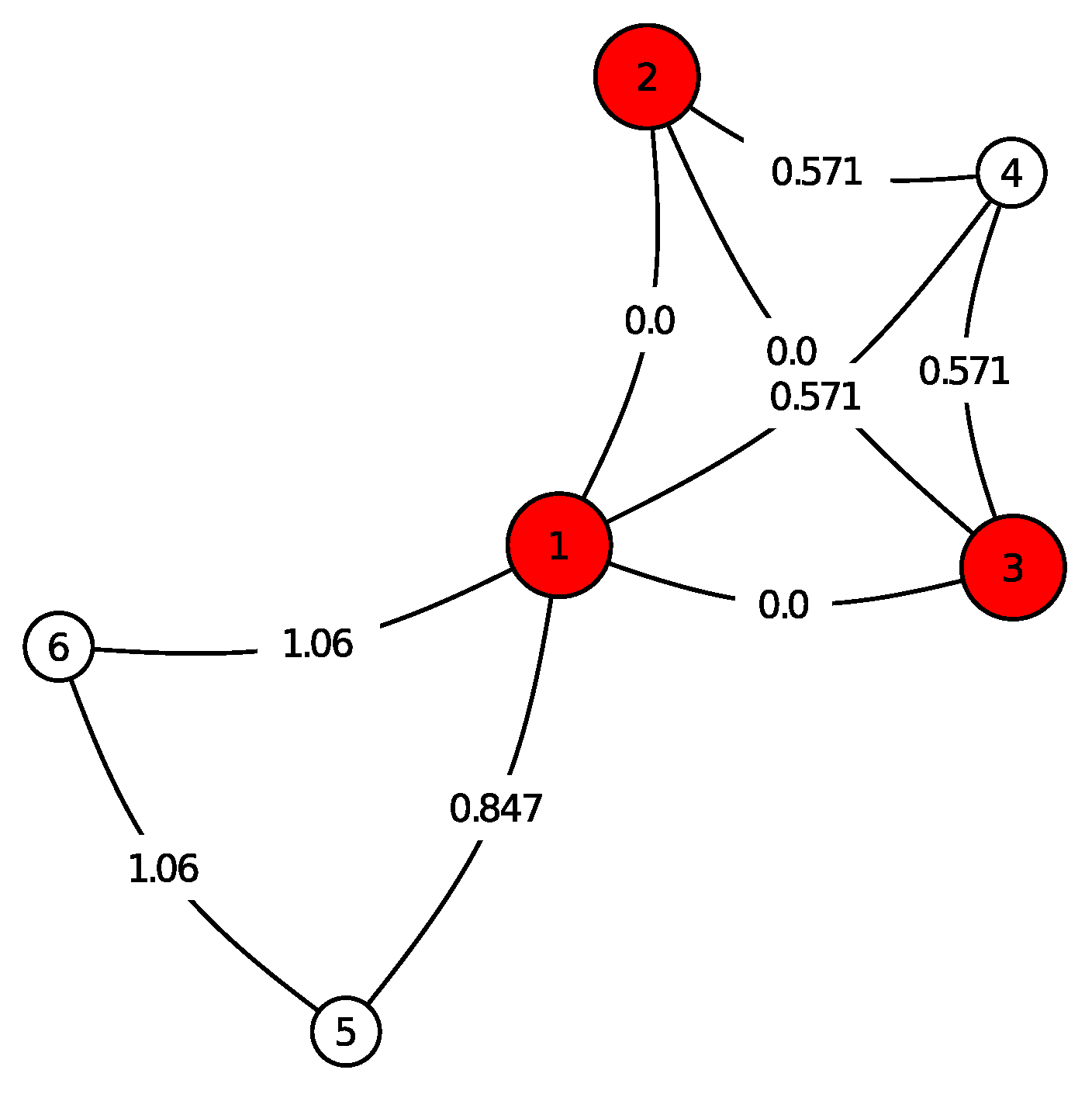
In Figure 1, an example is shown for our graph evolution model. For a clear view it contains only three birth steps after the initial time $t=0$. The nodes of the ancestor are highlighted by red. The edges are labelled with the birth times t. The following objects appear in Figure 1, which are described by the labels of their nodes:

• (1-2-3): is a triangle, the ancestor with birth time $t=0$,
• (1-2-3-4): represents three triangles, i.e., the offspring of (1-2-3) at its first reproduction time $t=0.571$,
• (1-5): an edge, offspring of (1-2-3) with birth time $t=0.847$,
• (1-5-6): a triangle, offspring of (1-5) with birth time $t=1.06$.

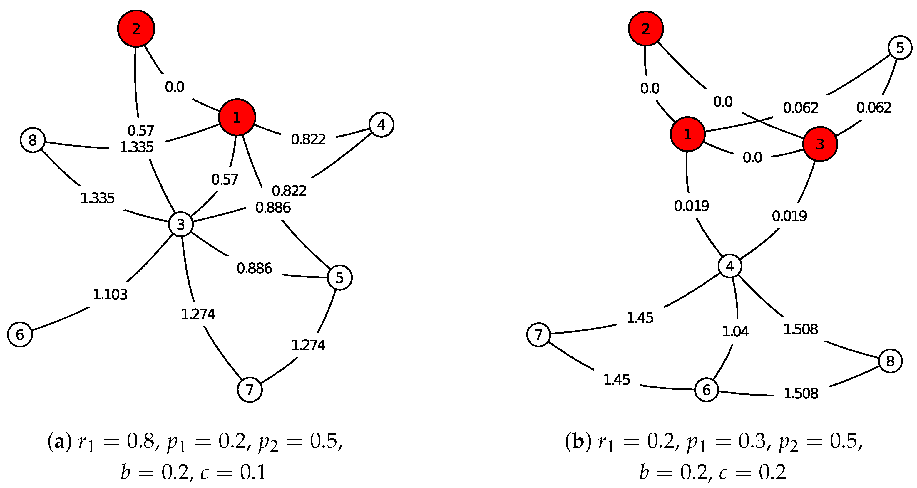
Two more examples are shown in Figure 2 with different parameters. In Figure 2a the ancestor is an edge, while in Figure 2b the ancestor is a triangle.

3. General Results

The survival functions.

Theorem 1.

The survival function for a triangle is

$$\mathbb{P}\left({\lambda }_3>t\right)=e^{-t\left(b+1\right)}{e}^{\frac{3(p_1+p_2)\left(1-e^{-ct}\right)+p_3\left(1-e^{-3ct}\right)}{3c}}.$$

(8)

The survival function for an edge is

$$\mathbb{P}\left({\lambda }_2>t\right)=e^{-t\left(b+1\right)}{e}^{\frac{1-e^{-ct}}{c}}.$$

(9)

Proof. 

At the first part of the proof we omit subscripts 2 and 3, because the calculations are the same for edges and triangles. Let $t>0$ and assume that $\Pi \left(t\right)=k$. Then, the first k birth events happened before time t. Thus, the birth times $\tau \left(1\right),\tau \left(2\right),\dots ,\tau \left(k\right)$ and the corresponding litter sizes $\epsilon \left(1\right),\epsilon \left(2\right),\dots ,\epsilon \left(k\right)$ are known. Therefore, the reproduction process $\xi \left(u\right)$ is also known for $u<t$. By (5), a simple calculation shows that the survival function of an object is

$$1-L\left(t\right)=exp\left(-{\int }_0^{t}l\left(u\right)du\right)=exp\left(-\left(bt+c{\int }_0^t\xi \left(u\right)du\right)\right)=$$

$$=exp\left(-\left(bt+ctS\left(k\right)-c\left(\epsilon \left(1\right)\tau \left(1\right)+\cdots +\epsilon \left(k\right)\tau \left(k\right)\right)\right)\right).$$

Then

$$\mathbb{P}\left(\lambda >t|\Pi \left(t\right)=k,\tau \left(1\right),\dots ,\tau \left(k\right),\epsilon \left(1\right),\dots ,\epsilon \left(k\right)\right)=$$

$$=exp\left(-\left(bt+ctS\left(k\right)-c\left(\epsilon \left(1\right)\tau \left(1\right)+\cdots +\epsilon \left(k\right)\tau \left(k\right)\right)\right)\right).$$

Let $\left(U_1^{\ast },\dots ,U_k^{\ast }\right)$ be an ordered sample of size k from uniform distribution on $\left[0,1\right]$. Then, the joint conditional distribution of the birth times $\tau \left(1\right),\dots ,\tau \left(k\right)$ given $\Pi \left(t\right)=k$, coincides with the distribution of $\left(t{U}_1^{\ast },\dots ,t{U}_k^{\ast }\right)$. Therefore

$$\mathbb{P}\left(\lambda >t|\Pi \left(t\right)=k\right)=\mathbb{E}exp\left(-\left(bt+ct\sum _{i=1}^k\epsilon \left(i\right)\left(1-{\displaystyle \frac{\tau \left(i\right)}{t}}\right)\right)\right)=$$

$$=\mathbb{E}exp\left(-bt+ct\sum _{i=1}^k\epsilon \left(i\right)\left(U_i^{\ast }-1\right)\right),$$

because $\tau \left(i\right)=t{U}_i^{\ast }$. The litter sizes $\epsilon \left(1\right),\dots ,\epsilon \left(k\right)$ are independent identically distributed random variables, which are independent also of $U_1^{\ast },\dots ,U_k^{\ast }$. Hence

$$\mathbb{P}\left(\lambda >t|\Pi \left(t\right)=k\right)=\mathbb{E}exp\left(-bt+ct\sum _{i=1}^k\epsilon \left(i\right)\left(U_i-1\right)\right)=$$

$$=e^{-bt}\mathbb{E}\prod _{i=1}^k{e}^{ct\epsilon \left(i\right)\left(U_i-1\right)}=e^{-bt}{\left({\mathbb{E}}_{\epsilon \left(i\right)}\left({\mathbb{E}}_{U_i}\left(e^{ct\epsilon \left(i\right)U_i}\right)e^{-ct\epsilon \left(i\right)}\right)\right)}^k=$$

$$=e^{-bt}{\left(\sum _{j=1}^{\infty }{q}_j{\displaystyle \frac{e^{ctj}-1}{ctj}}{e}^{-ctj}\right)}^k=e^{-bt}{\left(\sum _{j=1}^{\infty }{q}_j{\displaystyle \frac{1-e^{-ctj}}{ctj}}\right)}^k,$$

where we applied that $U_i$ is uniformly distributed. Using this and the total probability theorem, we find

$$\mathbb{P}\left(\lambda >t\right)=\sum _{k=0}^{\infty }\mathbb{P}\left(\Pi \left(t\right)=k\right)\mathbb{P}\left(\lambda >t|\Pi \left(t\right)=k\right)=$$

$$=\sum _{k=0}^{\infty }{\displaystyle \frac{t^k}{k!}}{e}^{-t}{e}^{-bt}{\left(\sum _{j=1}^{\infty }{q}_j{\displaystyle \frac{1-e^{-ctj}}{ctj}}\right)}^k=$$

$$=e^{-(b+1)t}\sum _{k=0}^{\infty }{\displaystyle \frac{1}{k!}}{\left(\sum _{j=1}^{\infty }{q}_j{\displaystyle \frac{1-e^{-ctj}}{cj}}\right)}^k=$$

$$=e^{-(b+1)t}{e}^{{\sum }_{j=1}^{\infty }{q}_j\frac{1-e^{-ctj}}{cj}}.$$

Therefore, the survival function for a triangle is

$$\mathbb{P}\left({\lambda }_3>t\right)=e^{-t\left(b+1\right)}{e}^{\frac{3(p_1+p_2)\left(1-e^{-ct}\right)+p_3\left(1-e^{-3ct}\right)}{3c}}.$$

Finally, the survival function for an edge is

$$\mathbb{P}\left({\lambda }_2>t\right)=e^{-t\left(b+1\right)}{e}^{\frac{1-e^{-ct}}{c}}.$$

□

The mean offspring number. Let us denote by $m_{i,j}\left(t\right)=\mathbb{E}{\xi }_{i,j}\left(t\right)$ the expectation of the number of type j offspring of a type i mother until time t.

Corollary 1.

For any $t\ge 0$, we have

$$m_{2,2}\left(t\right)=r_{1}F\left(t\right),m_{2,3}\left(t\right)=r_{2}F\left(t\right),$$

(10)

where

$$F\left(t\right)={\int }_0^t\left(1-L_2\left(s\right)\right)ds={\int }_0^t{e}^{-(b+1)s}{e}^{\frac{1-e^{-cs}}{c}}ds={\displaystyle \frac{1}{c}}{\int }_0^{1-e^{-ct}}{\left(1-u\right)}^{\frac{b+1}{c}-1}{e}^{\frac{u}{c}}du.$$

$$\mathbb{E}{\lambda }_2={\displaystyle \frac{1}{c}}{\int }_0^1{\left(1-u\right)}^{\frac{b+1}{c}-1}{e}^{\frac{u}{c}}du.$$

(11)

For any $t\ge 0$, we have

$$m_{3,2}\left(t\right)=p_{1}G\left(t\right),m_{3,3}\left(t\right)=(p_2+3p_3)G\left(t\right),$$

(12)

where

$$G\left(t\right)={\int }_0^t\left(1-L_3\left(s\right)\right)ds={\int }_0^t{e}^{-s\left(b+1\right)}{e}^{\frac{3(p_1+p_2)\left(1-e^{-cs}\right)+p_3\left(1-e^{-3cs}\right)}{3c}}ds=$$

$$={\displaystyle \frac{1}{c}}{\int }_0^{1-e^{-ct}}{\left(1-u\right)}^{\frac{b+1}{c}-1}{e}^{\frac{u}{3c}\left(p_3{u}^2-3p_{3}u+3\right)}du.$$

$$\mathbb{E}{\lambda }_3={\displaystyle \frac{1}{c}}{\int }_0^1{\left(1-u\right)}^{\frac{b+1}{c}-1}{e}^{\frac{u}{3c}\left(p_3{u}^2-3p_{3}u+3\right)}du.$$

(13)

$0<\mathbb{E}{\lambda }_2,\mathbb{E}{\lambda }_3<\infty$ because $b\ge 0$.

Proof. 

We have

$$m_{i,j}\left(t\right)=\mathbb{E}{\xi }_{i,j}\left(t\right)=\mathbb{E}\left({\epsilon }_{i,j}\left(1\right)+{\epsilon }_{i,j}\left(2\right)+\cdots +{\epsilon }_{i,j}\left(\Pi \left(t\wedge {\lambda }_i\right)\right)\right),$$

where ${\epsilon }_{i,j}\left(k\right)$ is the number of type j offspring of a type i mother at her kth birth event. Using Wald’s identity, the average number of children is

$$m_{i,j}\left(t\right)=\mathbb{E}\left({\epsilon }_{i,j}\left(1\right)\right)\mathbb{E}\left(\Pi \left(t\wedge {\lambda }_i\right)\right).$$

(14)

Using that $\Pi$ is a Poisson process with rate 1, and $t\wedge \lambda$ is bounded for any t, from (14), we obtain that the average number of children is

$$m_{i,j}\left(t\right)=\mathbb{E}\left({\epsilon }_{i,j}\left(1\right)\right)\mathbb{E}\left(t\wedge {\lambda }_i\right)=\mathbb{E}\left({\epsilon }_{i,j}\left(1\right)\right){\int }_0^t\left(1-L_i\left(s\right)\right)ds.$$

(15)

Now, consider $m_{2,2}\left(t\right)$. Applying (9) and using the substitution $u=1-e^{-cs}$, we obtain

$$m_{2,2}\left(t\right)=r_1{\int }_0^t{e}^{-(b+1)s}{e}^{\frac{1-e^{-cs}}{c}}ds={\displaystyle \frac{r_1}{c}}{\int }_0^{1-e^{-ct}}{\left(1-u\right)}^{\frac{b+1}{c}-1}{e}^{\frac{u}{c}}du.$$

(16)

If we write $r_2$ instead of $r_1$, then we obtain $m_{2,3}\left(t\right)$. Thus, we obtained (10). Moreover, with $t\to \infty$, we have $\mathbb{E}{\lambda }_2={\int }_0^{\infty }\mathbb{P}\left({\lambda }_2>t\right)dt$. Thus, (11) follows from (16).

Now, we turn to $m_{3,3}\left(t\right)$. Applying (8), and using the substitution $u=1-e^{-cs}$, we obtain,

$$\begin{gathered} {\int }_0^t\mathbb{P}\left({\lambda }_3>s\right)ds={\int }_0^t{e}^{-s\left(b+1\right)}{e}^{\frac{3(p_1+p_2)\left(1-e^{-cs}\right)+p_3\left(1-e^{-3cs}\right)}{3c}}ds= \\ ={\displaystyle \frac{1}{c}}{\int }_0^{1-e^{-ct}}{\left(1-u\right)}^{\frac{b+1}{c}-1}{e}^{\frac{u}{3c}\left(p_3{u}^2-3p_{3}u+3\left(p_1+p_2+p_3\right)\right)}du. \end{gathered}$$

(17)

As $\mathbb{E}\left({\epsilon }_{3,3}\left(1\right)\right)=p_2+3p_3$, so from (15) we obtain $m_{3,3}\left(t\right)$. Using that $\mathbb{E}\left({\epsilon }_{3,2}\left(1\right)\right)=p_1$, we obtain $m_{3,2}\left(t\right)$. Thus, we obtained (12). Moreover, we have $\mathbb{E}{\lambda }_3={\int }_0^{\infty }\mathbb{P}\left({\lambda }_3>t\right)dt$. Thus, (13) follows from (17) with $t\to \infty$. □

Let

$$m_{i,j}^{\ast }\left(\kappa \right)={\int }_0^{\infty }{e}^{-\kappa t}{m}_{i,j}\left(dt\right),i,j=2,3,$$

be the Laplace transform of $m_{i,j}$.

Proposition 1.

For any $\kappa \ge 0$, we have

$$m_{2,2}^{\ast }\left(\kappa \right)=r_{1}A\left(\kappa \right),m_{2,3}^{\ast }\left(\kappa \right)=r_{2}A\left(\kappa \right),$$

(18)

where

$$A\left(\kappa \right)={\int }_0^{\infty }{e}^{-\kappa s}{e}^{-(b+1)s}{e}^{\frac{1-e^{-cs}}{c}}ds={\displaystyle \frac{1}{c}}{\int }_0^1{\left(1-u\right)}^{\frac{\kappa +b+1}{c}-1}{e}^{\frac{u}{c}}du.$$

(19)

For any $\kappa \ge 0$, we have

$$m_{3,2}^{\ast }\left(\kappa \right)=p_{1}B\left(\kappa \right),m_{3,3}^{\ast }\left(\kappa \right)=(p_2+3p_3)B\left(\kappa \right),$$

(20)

where

$$B\left(\kappa \right)={\int }_0^{\infty }{e}^{-\kappa s}{e}^{-s\left(b+1\right)}{e}^{\frac{3(p_1+p_2)\left(1-e^{-cs}\right)+p_3\left(1-e^{-3cs}\right)}{3c}}ds=$$

$$={\displaystyle \frac{1}{c}}{\int }_0^1{\left(1-u\right)}^{\frac{\kappa +b+1}{c}-1}{e}^{\frac{u}{3c}\left(p_3{u}^2-3p_{3}u+3\right)}du.$$

Proof. 

Apply the definition of $m_{i,j}^{\ast }\left(\kappa \right)$, Corollary 1 and substitution $u=1-e^{-cs}$. □

The Perron root and the Malthusian parameter. Let

$$M\left(\kappa \right)=\left(\begin{array}{cc}{m}_{2,2}^{\ast }\left(\kappa \right)& m_{2,3}^{\ast }\left(\kappa \right)\\ m_{3,2}^{\ast }\left(\kappa \right)& m_{3,3}^{\ast }\left(\kappa \right)\end{array}\right)$$

(21)

be the matrix of the Laplace transforms. Direct calculation gives that the characteristic roots of $M\left(\kappa \right)$ are

$${\varrho }_{1,2}\left(\kappa \right)=\frac{(p_2+3p_3)B\left(\kappa \right)+r_{1}A\left(\kappa \right)\pm \sqrt{{((p_2+3p_3)B\left(\kappa \right)-r_{1}A\left(\kappa \right))}^2+4p_{1}B\left(\kappa \right)r_{2}A\left(\kappa \right)}}{2}.$$

(22)

The greater of the values ${\varrho }_1\left(\kappa \right)$ and ${\varrho }_2\left(\kappa \right)$ is called the Perron root, so

$$\varrho \left(\kappa \right)={\varrho }_1\left(\kappa \right)=\frac{(p_2+3p_3)B\left(\kappa \right)+r_{1}A\left(\kappa \right)+\sqrt{{((p_2+3p_3)B\left(\kappa \right)-r_{1}A\left(\kappa \right))}^2+4p_{1}B\left(\kappa \right)r_{2}A\left(\kappa \right)}}{2}$$

(23)

is the Perron root.

We assume that our process is supercritical; that is,

$$\varrho \left(0\right)>1.$$

(24)

For supercriticality, condition

$$max\{(p_2+3p_3)B\left(0\right),r_{1}A\left(0\right)\}>1$$

is sufficient.

That value of $\kappa$ for which the Perron root is equal to 1 is called the Malthusian parameter. Thus, using the usual notation in the theory of branching processes, $\alpha$ is the Malthusian parameter if $\varrho \left(\alpha \right)=1$. In this paper, we assume the existence of the Malthusian parameter. From relation $\varrho \left(\alpha \right)=1$ and (23), we obtain that the Malthusian $\alpha$ satisfies the equation

$$r_{1}A\left(\alpha \right)(p_2+3p_3)B\left(\alpha \right)-\left(r_{1}A\left(\alpha \right)+(p_2+3p_3)B\left(\alpha \right)\right)=r_{2}A\left(\alpha \right)p_{1}B\left(\alpha \right)-1.$$

(25)

Later, we use the eigenvectors of $M\left(\alpha \right)$. To this end, let $\alpha$ be the Malthusian parameter, and let ${(v_2,v_3)}^{\top }$ be the right eigenvector of $M\left(\alpha \right)$ corresponding to eigenvalue 1 and satisfying condition $v_2+v_3=1$. Then, direct calculation shows that

$$v_2=\frac{(r_1-1)A\left(\alpha \right)}{(2r_1-1)A\left(\alpha \right)-1},v_3=\frac{r_{1}A\left(\alpha \right)-1}{(2r_1-1)A\left(\alpha \right)-1}.$$

(26)

Again, let $\alpha$ be the Malthusian parameter and let ${(u_2,u_3)}^{\top }$ be the left eigenvector of $M\left(\alpha \right)$ satisfying condition $u_2{v}_2+u_3{v}_3=1$. Direct calculation shows that

$$u_2=\frac{p_{1}B\left(\alpha \right)\left((2r_1-1)A\left(\alpha \right)-1\right)}{p_{1}B\left(\alpha \right)(r_1-1)A\left(\alpha \right)-{(r_{1}A\left(\alpha \right)-1)}^2},u_3=\frac{(1-r_{1}A\left(\alpha \right))\left((2r_1-1)A\left(\alpha \right)-1\right)}{p_{1}B\left(\alpha \right)(r_1-1)A\left(\alpha \right)-{(r_{1}A\left(\alpha \right)-1)}^2}.$$

(27)

4. Asymptotic Theorems on the Number of Triangles and Edges

In this section, we use Proposition 4 from Section 8. So we should check the conditions given in Section 8. For condition (a) from Section 8, we should guarantee that not all measures $m_{i,j}$ are concentrated on a lattice. By Corollary 1, these measures are absolutely continuous, and thus it is satisfied.

Concerning condition (b1), we underline that we suppose the existence of a positive Malthusian parameter $\alpha$. To this end, in this section, we assume that (25) has a finite positive solution $\alpha$. We can check numerically the existence of this value. For (b2), we assume (24). Condition (c) from Section 8 will be checked later in the proofs of the results together with other conditions related to it.

Now, we analyse condition (d). We can see from Corollary 1 that $F(\infty )$ and $G(\infty )$ are positive. Thus, we can concentrate on parameters $r_i$ and $p_i$. If $r_2=p_1=0$, then (d) is not satisfied; however, in this case, one can study separately the process of edges (it grows at any birth time by 1), and the process of triangles (this is described in [17]). If $r_1=0$ and $p_2+p_3=0$, then (d) is not satisfied, and the evolution process is an alternating one. If either $r_2=0$ or $p_1=0$, then (d) is not satisfied.

To guarantee condition (d), in this section, we assume that $0\le r_1<1$, $0<p_1\le 1$, and it is excluded that both $r_1=0$ and $p_1=1$ are satisfied at the same time. In this case, condition (d) from Section 8 is satisfied.

The denominator in the limit theorem. In the following theorem, we need the next formulae. In Section 8, we see that the denominator of $m_{\infty }^{\Phi }$ in the limiting expression is independent of $\Phi$, and it is

$$\sum _{l,j=1}^p{u}_l{v}_j{\int }_0^{\infty }t{e}^{-\alpha t}{m}_{l,j}\left(dt\right).$$

It can be written in the form (and considering our two-dimensional case)

$$D\left(\alpha \right)=\sum _{l,j=2}^3{u}_l{v}_j{\left(-m_{l,j}^{\ast }\left(\alpha \right)\right)}^{\prime }.$$

(28)

Here, $u_i$ and $v_i$ are from Equations (26) and (27). Moreover, by Corollary 1 or by Proposition 1, we have that

$$\begin{array}{ccc}\hfill & {\left(-m_{2,2}^{\ast }\left(\alpha \right)\right)}^{\prime }=r_1\left(-A^{\prime }\left(\alpha \right)\right),& {\left(-m_{2,3}^{\ast }\left(\alpha \right)\right)}^{\prime }=r_2\left(-A^{\prime }\left(\alpha \right)\right),\hfill \end{array}$$

(29)

$$\begin{array}{ccc}& {\left(-m_{3,2}^{\ast }\left(\alpha \right)\right)}^{\prime }=p_1\left(-B^{\prime }\left(\alpha \right)\right),& {\left(-m_{3,3}^{\ast }\left(\alpha \right)\right)}^{\prime }=(p_2+3p_3)\left(-B^{\prime }\left(\alpha \right)\right),\hfill \end{array}$$

(30)

where

$$-A^{\prime }\left(\alpha \right)={\int }_0^{\infty }s{e}^{-\alpha s}{e}^{-(b+1)s}{e}^{\frac{1-e^{-cs}}{c}}ds=-{\displaystyle \frac{1}{c^2}}{\int }_0^{1}ln(1-u){\left(1-u\right)}^{\frac{\alpha +b+1}{c}-1}{e}^{\frac{u}{c}}du,$$

(31)

$$\begin{gathered} -B^{\prime }\left(\alpha \right)={\int }_0^{\infty }s{e}^{-\alpha s}{e}^{-s\left(b+1\right)}{e}^{\frac{3(p_1+p_2)\left(1-e^{-cs}\right)+p_3\left(1-e^{-3cs}\right)}{3c}}ds= \\ =-{\displaystyle \frac{1}{c^2}}{\int }_0^{1}ln(1-u){\left(1-u\right)}^{\frac{\alpha +b+1}{c}-1}{e}^{\frac{u}{3c}\left(p_3{u}^2-3p_{3}u+3\right)}du. \end{gathered}$$

(32)

Now, we turn to the number of edges and triangles. Recall that an edge is a type 2, and a triangle is a type 3 object.

Theorem 2.

Assume that (24) is satisfied and (25) has a finite positive solution α. Assume that $0\le r_1<1$, $0<p_1\le 1$ and it is excluded that both $r_1=0$ and $p_1=1$ are satisfied at the same time.

Let ${}_{i}E\left(t\right)$ denote the number of all edges being born up to time t if the ancestor of the population was a type i object, $i=2,3$. Then

$$\underset{t\to \infty }{lim}{e}^{-\alpha t}{}_{i}E\left(t\right)={}_{i}W\frac{v_i{u}_2}{\alpha D\left(\alpha \right)}$$

(33)

almost surely for $i=2,3$.

Let ${}_i\widehat{E}\left(t\right)$ denote the number of all edges present at time t if the ancestor of the population was a type i object, $i=2,3$. Then

$$\underset{t\to \infty }{lim}{e}^{-\alpha t}{}_i\widehat{E}\left(t\right)={}_{i}W\frac{v_i{u}_{2}A\left(\alpha \right)}{D\left(\alpha \right)}$$

(34)

almost surely for $i=2,3$.

Let ${}_{i}T\left(t\right)$ denote the number of all triangles being born up to time t if the ancestor of the population was a type i object, $i=2,3$. Then

$$\underset{t\to \infty }{lim}{e}^{-\alpha t}{}_{i}T\left(t\right)={}_{i}W\frac{v_i{u}_3}{\alpha D\left(\alpha \right)}$$

(35)

almost surely for $i=2,3$.

Let ${}_i\widehat{T}\left(t\right)$ denote the number of all triangles present at time t if the ancestor of the population was a type i object, $i=2,3$. Then,

$$\underset{t\to \infty }{lim}{e}^{-\alpha t}{}_i\widehat{T}\left(t\right)={}_{i}W\frac{v_i{u}_{3}B\left(\alpha \right)}{D\left(\alpha \right)}$$

(36)

almost surely for $i=2,3$.

The quantities ${}_{2}W$ and ${}_{3}W$ are a.s. non-negative, $\mathbb{E}\left({}_{2}W\right)=\mathbb{E}\left({}_{3}W\right)=1$, ${}_{2}W$ and ${}_{3}W$ are a.s. positive on the event of survival.

Proof. 

We apply Proposition 4. To obtain condition (71), it is enough to show that

$$\mathbb{E}\left[{}_{\alpha }{\xi }_i(\infty ){log}^{+}{}_{\alpha }{\xi }_i(\infty )\right]<\infty ,i=2,3,$$

(37)

where

$${}_{\alpha }{\xi }_i(\infty )={\int }_0^{\infty }{e}^{-\alpha t}{\xi }_i\left(dt\right),i=2,3,$$

(38)

and

$${\xi }_i\left(t\right)={\xi }_{i,2}\left(t\right)+{\xi }_{i,3}\left(t\right),i=2,3.$$

(39)

If $i=2$, then ${\xi }_2\left(t\right)$ is the birth process of an edge, and the children can be both edges and triangles. Therefore, at each birth, there is one child. Therefore,

$${}_{\alpha }{\xi }_2(\infty )={\int }_0^{\infty }{e}^{-\alpha t}{\xi }_2\left(dt\right)=\sum _{\tau \left(i\right)\le {\lambda }_2}1e^{-\alpha \tau \left(i\right)}\le \sum _{i=1}^{\infty }1e^{-\alpha \tau \left(i\right)}=M,$$

where $\tau \left(1\right),\tau \left(2\right),\dots$ are the jumps of the Poisson process ${\Pi }_2$. In the Poisson process ${\Pi }_2\left(t\right)$ the distribution of the interarrival time ($\tau \left(i\right)-\tau \left(i-1\right)$) is exponential with rate 1. Therefore, $\tau \left(i\right)$ has $\Gamma$-distribution $\Gamma \left(i,1\right)$. Using this, we have

$$\mathbb{E}\left(M\right)=\sum _{i=1}^{\infty }\mathbb{E}\left(e^{-\alpha \tau \left(i\right)}\right)=\sum _{i=1}^{\infty }{\displaystyle \frac{1}{{\left(1+\alpha \right)}^i}}={\displaystyle \frac{1}{\alpha }}.$$

(40)

Let us denote by ${\eta }_i$ the interarrival time $\tau \left(i\right)-\tau \left(i-1\right)$. Let ${\eta }_0$ be an exponentially distributed random variable with rate 1 that is independent of M. Then,

$$e^{-\alpha {\eta }_0}\left(1+M\right)=e^{-\alpha {\eta }_0}+e^{-\alpha {\eta }_0}\sum _{i=1}^{\infty }{e}^{-\alpha \left({\eta }_1+\cdots +{\eta }_i\right)}=\sum _{i=0}^{\infty }{e}^{-\alpha \left({\eta }_0+{\eta }_1+\cdots +{\eta }_i\right)}.$$

Therefore, the distribution of $e^{-\alpha {\eta }_0}\left(1+M\right)$ coincides with the distribution of M. Therefore, using (40), we have

$$\mathbb{E}{M}^2=\mathbb{E}{\left(e^{-\alpha {\eta }_0}\left(1+M\right)\right)}^2={\displaystyle \frac{1}{1+2\alpha }}\left(1+\frac{2}{\alpha }+\mathbb{E}{M}^2\right).$$

From this, we find

$$\mathbb{E}{M}^2={\displaystyle \frac{\alpha +2}{2{\alpha }^2}}<\infty .$$

Thus, (37) is true for $i=2$.

If $i=3$, then ${\xi }_3\left(t\right)$ is the birth process of a triangle and the children can be both edges and triangles. Therefore, at each birth there are at most three children. Therefore,

$${}_{\alpha }{\xi }_3(\infty )={\int }_0^{\infty }{e}^{-\alpha t}{\xi }_3\left(dt\right)=\sum _{\tau \left(i\right)\le {\lambda }_3}\epsilon \left(i\right)e^{-\alpha \tau \left(i\right)}\le 3\sum _{i=1}^{\infty }1e^{-\alpha \tau \left(i\right)}=3M,$$

where $\tau \left(1\right),\tau \left(2\right),\dots$ are the jumps of the Poisson process ${\Pi }_3$. By the above calculation $\mathbb{E}{M}^2<\infty$, so (37) is true for $i=3$.

If we show that ${\int }_0^{\infty }{t}^2{e}^{-\alpha t}{m}_{i,j}\left(dt\right)<\infty$, for $i,j=2,3$, then conditions (c) and $\left(iv\right)$ of Section 8 will be proved. Now, for $i=2$ and $j=2,3$, we have from Corollary 1

$${\int }_0^{\infty }{t}^2{e}^{-\alpha t}{m}_{2,j}\left(dt\right)\le max\{r_1,r_2\}{\int }_0^{\infty }{t}^2{e}^{-\alpha t}{e}^{-t\left(b+1\right)}{e}^{\frac{1-e^{-ct}}{c}}dt\le {\int }_0^{\infty }{t}^2{e}^{-t(\alpha +b+1-1)}dt<\infty$$

because $\alpha +b>0$.

For $i=3$ and $j=2,3$, we have from Corollary 1

$${\int }_0^{\infty }{t}^2{e}^{-\alpha t}{m}_{3,j}\left(dt\right)\le max\{p_1,p_2+3p_3\}{\int }_0^{\infty }{t}^2{e}^{-\alpha t}{e}^{-t\left(b+1\right)}{e}^{(p_1+p_2)\frac{1-e^{-ct}}{c}+p_3\frac{1-e^{-3ct}}{3c}}dt\le$$

$$\le {\int }_0^{\infty }{t}^2{e}^{-t(\alpha +b+1-1)}dt<\infty$$

Thus, conditions (c) and $\left(iv\right)$ of Section 8 are proved.

Now, turn to the number of edges.

To obtain (33), let ${\Phi }_x\left(t\right)=1$ if x is an edge, and ${\Phi }_x\left(t\right)=0$ if x is a triangle. Therefore, $\mathbb{E}{\Phi }_2\left(t\right)=1$ and $\mathbb{E}{\Phi }_3\left(t\right)=0$. Conditions $\left(i\right)-\left(ii\right)-\left(iii\right)$ and $\left(v\right)$ of Section 8 are satisfied. Thus, (69) and (70) imply (33).

To obtain (34), let ${\Phi }_x\left(t\right)=1$ if x is an edge and it is present at t, and ${\Phi }_x\left(t\right)=0$ if x is a triangle. Therefore, $\mathbb{E}{\Phi }_2\left(t\right)=1-L_2\left(t\right)$ and $\mathbb{E}{\Phi }_3\left(t\right)=0$. Conditions $\left(i\right)-\left(ii\right)-\left(iii\right)$ and $\left(v\right)$ of Section 8 are satisfied. Now,

$${\int }_0^{\infty }{e}^{-\alpha t}\mathbb{E}{\Phi }_2\left(t\right)dt={\int }_0^{\infty }{e}^{-\alpha t}(1-L_2\left(t\right))dt=A\left(\alpha \right).$$

Thus, (69) and (70) imply (34).

Now, we turn to the number of triangles.

To obtain (35), let ${\Phi }_x\left(t\right)=0$ if x is an edge, and ${\Phi }_x\left(t\right)=1$ if x is a triangle. Therefore, $\mathbb{E}{\Phi }_2\left(t\right)=0$ and $\mathbb{E}{\Phi }_3\left(t\right)=1$. Conditions $\left(i\right)-\left(ii\right)-\left(iii\right)$ and $\left(v\right)$ of Section 8 are satisfied. Thus, (69) and (70) imply (35).

To obtain (36), let ${\Phi }_x\left(t\right)=0$ if x is an edge, and ${\Phi }_x\left(t\right)=1$ if x is a triangle, and it is present at t. Therefore, $\mathbb{E}{\Phi }_2\left(t\right)=0$ and $\mathbb{E}{\Phi }_3\left(t\right)=1-L_3\left(t\right)$. Conditions $\left(i\right)-\left(ii\right)-\left(iii\right)$ and $\left(v\right)$ of Section 8 are satisfied. Now,

$${\int }_0^{\infty }{e}^{-\alpha t}\mathbb{E}{\Phi }_3\left(t\right)dt={\int }_0^{\infty }{e}^{-\alpha t}(1-L_3\left(t\right))dt=B\left(\alpha \right).$$

Thus, (69) and (70) imply (36). □

5. Generating Functions and the Probability of Extinction

The joint generating function of ${\Pi }_2\left({\lambda }_2\right)$, ${\xi }_{22}\left({\lambda }_2\right)$ and ${\xi }_{23}\left({\lambda }_2\right)$. Recall that ${\Pi }_2$ is the Poisson process describing the reproduction times of the generic edge and ${\lambda }_2$ is its life length. Thus,

$$w_{i,j,k}=\mathbb{P}\left({\Pi }_2\left({\lambda }_2\right)=i,{\xi }_{22}\left({\lambda }_2\right)=j,{\xi }_{23}\left({\lambda }_2\right)=k\right)$$

is the joint distribution of the offspring size of the generic edge during its whole life and its last reproduction time. We have

$$w_{i,j,k}=\mathbb{P}\left({\tau }_i\le {\lambda }_2<{\tau }_{i+1},{\xi }_{22}\left({\tau }_i\right)=j,{\xi }_{23}\left({\tau }_i\right)=k\right),$$

where ${\tau }_i$ is the ith jumping time of the Poisson process ${\Pi }_2$. Thus, it again shows that $w_{i,j,k}$ is the probability that the ith birth event is the last one that occurred before death, and the total numbers of the two types of offspring up to time ${\tau }_i$ are equal to j and k, respectively.

Now, consider the sequence

$$u_{i,j,k}=\mathbb{P}\left({\tau }_i\le {\lambda }_2,{\xi }_{22}\left({\tau }_i\right)=j,{\xi }_{23}\left({\tau }_i\right)=k\right).$$

Let ${\xi }_2\left({\tau }_{i-1}\right)=m$ and assume for a while that ${\tau }_i$ and ${\tau }_{i-1}$ are fixed. Then, using (4) and (5) for the hazard rate, we can calculate that, for fixed ${\tau }_i$ and ${\tau }_{i-1}$,

$$\mathbb{P}\left({\lambda }_2\ge {\tau }_i|{\lambda }_2\ge {\tau }_{i-1}\right)=exp\left(-\left(b+cm\right)\left({\tau }_i-{\tau }_{i-1}\right)\right).$$

We know that the increment $\left({\tau }_i-{\tau }_{i-1}\right)$ is exponential with parameter 1; therefore,

$$\mathbb{P}\left({\lambda }_2\ge {\tau }_i|{\lambda }_2\ge {\tau }_{i-1}\right)={\mathbb{E}}_{{\tau }_i-{\tau }_{i-1}}exp\left(-\left(b+cm\right)({\tau }_i-{\tau }_{i-1})\right)={\displaystyle \frac{1}{1+b+cm}}.$$

(41)

At each birth step, the new individual can be either an edge or a triangle. Therefore, using the above calculations, the total probability theorem, and the independence of the type of the newly born individual and $({\Pi }_2,{\lambda }_2)$, we have the following recursion for $u_{i,j,k}$.

$$u_{i,j,k}=u_{i-1,j-1,k}{\displaystyle \frac{r_1}{1+b+c(j+k-1)}}+u_{i-1,j,k-1}{\displaystyle \frac{r_2}{1+b+c\left(j+k-1\right)}}.$$

(42)

Now, by the definition of $w_{i,j,k}$, we can see that

$$\begin{array}{c}{w}_{i,j,k}=\mathbb{P}\left({\tau }_i\le {\lambda }_2<{\tau }_{i+1},{\xi }_{22}\left({\tau }_i\right)=j,{\xi }_{23}\left({\tau }_i\right)=k\right)=\hfill \\ =\mathbb{P}\left({\lambda }_2<{\tau }_{i+1}|{\tau }_i\le {\lambda }_2,{\xi }_{22}\left({\tau }_i\right)=j,{\xi }_{23}\left({\tau }_i\right)=k\right)\mathbb{P}\left({\tau }_i\le {\lambda }_2,{\xi }_{22}\left({\tau }_i\right)=j,{\xi }_{23}\left({\tau }_i\right)=k\right)=\\ \hfill ={\displaystyle \frac{b+c(j+k)}{1+b+c(j+k)}}{u}_{i,j,k},\end{array}$$

where by (41), $\frac{b+c(j+k)}{1+b+c(j+k)}$ is the probability that the generic individual dies before the next birth event.

Let $v_{i,j,k}={\displaystyle \frac{w_{i,j,k}}{b+c(j+k)}}={\displaystyle \frac{u_{i,j,k}}{1+b+c(j+k)}}$. Then, from (42), we obtain the following recursion for the sequence $v_{i,j,k}$

$$\left(1+b+c(j+k)\right)v_{i,j,k}=v_{i-1,j-1,k}{r}_1+v_{i-1,j,k-1}{r}_2,$$

(43)

where the initial values are

$$v_{0,0,0}={\displaystyle \frac{1}{1+b}}\mathrm{and}{v}_{0,j,k}=0\mathrm{for}j\ne 0\mathrm{or}k\ne 0.$$

(44)

Now, we calculate the generating function $G\left(x,y,z\right)$ of the sequence $v_{i,j,k}$. We have

$$G\left(x,y,z\right)=\sum _{i=0}^{\infty }\sum _{j=0}^{\infty }\sum _{k=0}^{\infty }{v}_{i,j,k}{x}^i{y}^j{z}^k.$$

First, multiplying with $x^i{y}^j{z}^k$ and then taking the sum of both sides of (43), we obtain

$$\begin{array}{c}\sum _{i=1}^{\infty }\sum _{j=0}^{\infty }\sum _{k=0}^{\infty }{v}_{i,j,k}{x}^i{y}^j{z}^k\left(1+b+cj+ck\right)=\hfill \\ \hfill \hspace{1em}\hspace{1em}\hspace{1em}\hspace{1em}\hspace{1em}=r_{1}xy\sum _{i=1}^{\infty }\sum _{j=0}^{\infty }\sum _{k=0}^{\infty }{v}_{i-1,j-1,k}{x}^{i-1}{y}^{j-1}{z}^k+r_{2}xz\sum _{i=1}^{\infty }\sum _{j=0}^{\infty }\sum _{k=0}^{\infty }{v}_{i-1,j,k-1}{x}^{i-1}{y}^j{z}^{k-1},\end{array}$$

where $v_{0,j,k},j=0,1,\dots$ is given by (44), and we define $v_{i,j,k}=0$ if $j<0$ or $k<0$. From this equation, we find

$$\begin{array}{c}\left(1+b\right)\left(G\left(x,y,z\right)-{\displaystyle \frac{1}{1+b}}\right)+yc{G}_y^{{}^{\prime }}\left(x,y,z\right)+zc{G}_z^{{}^{\prime }}\left(x,y,z\right)=\hfill \\ \hfill \hspace{1em}\hspace{1em}\hspace{1em}\hspace{1em}\hspace{1em}\hspace{1em}\hspace{1em}\hspace{1em}\hspace{1em}\hspace{1em}\hspace{1em}\hspace{1em}\hspace{1em}\hspace{1em}\hspace{1em}\hspace{1em}\hspace{1em}=r_{1}xyG\left(x,y,z\right)+r_{2}xzG\left(x,y,z\right).\end{array}$$

(45)

Let $h\left(t\right)=G\left(x,ty,tz\right)$. Now, substituting y with $ty$, z with $tz$ in (45), we can obtain the following linear differential equation.

$$h^{{}^{\prime }}\left(t\right)+h\left(t\right)\left({\displaystyle \frac{1+b}{ct}}-\frac{r_{1}xy+r_{2}xz}{c}\right)={\displaystyle \frac{1}{ct}}$$

(46)

with the initial value condition

$$h\left(0\right)={\displaystyle \frac{1}{1+b}}.$$

(47)

Now, we can use the well-known method for linear differential equations. We obtain that the solution of the initial value problem (46) and (47) is

$$h\left(t\right)=t^{-\frac{1+b}{c}}{e}^{\frac{r_{1}xy+r_{2}xz}{c}t}{\displaystyle \frac{1}{c}}{\int }_0^t{s}^{\frac{1+b-c}{c}}{e}^{-\frac{r_{1}xy+r_{2}xz}{c}s}ds.$$

With $t=1$, we obtain that

$$G\left(x,y,z\right)=h\left(1\right)={\displaystyle \frac{1}{c}}{\int }_0^1{s}^{\frac{1+b-c}{c}}{e}^{\frac{r_{1}xy+r_{2}xz}{c}(1-s)}ds.$$

We need the generating function of $w_{i,j,k}=v_{i,j,k}(b+c(j+k))$. It is

$$H\left(x,y,z\right)=\sum _{i=0}^{\infty }\sum _{j=0}^{\infty }\sum _{k=0}^{\infty }{v}_{i,j,k}(b+c(j+k))x^i{y}^j{z}^k=$$

$$=bG\left(x,y,z\right)+cy{G}_y^{\prime }\left(x,y,z\right)+cz{G}_z^{\prime }\left(x,y,z\right).$$

(48)

From here, we obtain

Proposition 2.

The joint generating function of ${\Pi }_2\left({\lambda }_2\right)$, ${\xi }_{22}\left({\lambda }_2\right)$ and ${\xi }_{23}\left({\lambda }_2\right)$ is

$$\begin{array}{c}H\left(x,y,z\right)=\hfill \\ \hfill \hspace{1em}\hspace{1em}\hspace{1em}\hspace{1em}\hspace{1em}\hspace{1em}\hspace{1em}\hspace{1em}{e}^{\frac{r_{1}xy+r_{2}xz}{c}}{\displaystyle \frac{1}{c}}{\int }_0^1{s}^{\frac{1+b-c}{c}}{e}^{-\frac{r_{1}xy+r_{2}xz}{c}s}\left[b+(r_{1}xy+r_{2}xz)(1-s)\right]ds,\end{array}$$

(49)

where $-1\le x,y,z\le 1$.

Corollary 2.

The generating function of the total offspring distribution of the generic edge is

$$f_2(y,z)=H\left(1,y,z\right)=e^{\frac{r_{1}y+r_{2}z}{c}}{\displaystyle \frac{1}{c}}{\int }_0^1{s}^{\frac{1+b-c}{c}}{e}^{-\frac{r_{1}y+r_{2}z}{c}s}\left[b+(r_{1}y+r_{2}z)(1-s)\right]ds.$$

(50)

The joint generating function of ${\Pi }_3\left({\lambda }_3\right)$, ${\xi }_{32}\left({\lambda }_3\right)$ and ${\xi }_{33}\left({\lambda }_3\right)$. Here, we study the offspring of a triangle. To distinguish the notation of this subsection and the previous subsection, but avoid too many subscripts, we use bar. Thus, here ${\overline{w}}_{i,j,k}$, ${\overline{u}}_{i,j,k}$, ${\overline{v}}_{i,j,k}$, $\overline{G}(x,y,z)$ and $\overline{H}(x,y,z)$ denote quantities relating offspring of the generic triangle. Recall that ${\Pi }_3$ is the Poisson process describing the reproduction times of the generic triangle and ${\lambda }_3$ is the life length of the triangle. Thus,

$${\overline{w}}_{i,j,k}=\mathbb{P}\left({\Pi }_3\left({\lambda }_3\right)=i,{\xi }_{32}\left({\lambda }_3\right)=j,{\xi }_{33}\left({\lambda }_3\right)=k\right)$$

is the joint distribution of the offspring size of the generic triangle during its whole life and its last reproduction time. We have

$${\overline{w}}_{i,j,k}=\mathbb{P}\left({\tau }_i\le {\lambda }_3<{\tau }_{i+1},{\xi }_{32}\left({\tau }_i\right)=j,{\xi }_{33}\left({\tau }_i\right)=k\right),$$

where ${\tau }_i$ is the ith jumping time of the Poisson process ${\Pi }_3$. Thus, we again show that ${\overline{w}}_{i,j,k}$ is the probability that the ith birth event is the last one that happened before death, and the total numbers of the two types of offspring up to time ${\tau }_i$ are equal to j and k, respectively.

Let

$${\overline{u}}_{i,j,k}=\mathbb{P}\left({\tau }_i\le {\lambda }_3,{\xi }_{32}\left({\tau }_i\right)=j,{\xi }_{33}\left({\tau }_i\right)=k\right).$$

Let ${\xi }_3\left({\tau }_{i-1}\right)=m$, and assume for a while that ${\tau }_i$ and ${\tau }_{i-1}$ are fixed. Then, using (4) and (5) for the hazard rate, we can calculate that, for fixed ${\tau }_i$ and ${\tau }_{i-1}$,

$$\mathbb{P}\left({\lambda }_3\ge {\tau }_i|{\lambda }_3\ge {\tau }_{i-1}\right)=exp\left(-\left(b+cm\right)\left({\tau }_i-{\tau }_{i-1}\right)\right).$$

We know that the increment $\left({\tau }_i-{\tau }_{i-1}\right)$ is exponential with parameter 1; therefore,

$$\mathbb{P}\left({\lambda }_3\ge {\tau }_i|{\lambda }_3\ge {\tau }_{i-1}\right)={\mathbb{E}}_{{\tau }_i-{\tau }_{i-1}}exp\left(-\left(b+cm\right)({\tau }_i-{\tau }_{i-1})\right)={\displaystyle \frac{1}{1+b+cm}}.$$

(51)

At each birth step, the new individual can be either an edge or a triangle. Therefore, using the above calculations, the total probability theorem, and the independence of the type of the newly born individual and $({\Pi }_3,{\lambda }_3)$, we have the following recursion for ${\overline{u}}_{i,j,k}$.

$$\begin{array}{c}{\overline{u}}_{i,j,k}={\overline{u}}_{i-1,j-1,k}{\displaystyle \frac{p_1}{1+b+c(j+k-1)}}+\hfill \\ \hfill \hspace{1em}\hspace{1em}\hspace{1em}\hspace{1em}\hspace{1em}\hspace{1em}\hspace{1em}+{\overline{u}}_{i-1,j,k-1}{\displaystyle \frac{p_2}{1+b+c\left(j+k-1\right)}}+{\overline{u}}_{i-1,j,k-3}{\displaystyle \frac{p_3}{1+b+c\left(j+k-3\right)}}.\end{array}$$

(52)

Now, by the definition of ${\overline{w}}_{i,j,k}$, we can see that

$$\begin{array}{c}{\overline{w}}_{i,j,k}=\mathbb{P}\left({\tau }_i\le {\lambda }_3<{\tau }_{i+1},{\xi }_{32}\left({\tau }_i\right)=j,{\xi }_{33}\left({\tau }_i\right)=k\right)=\hfill \\ =\mathbb{P}\left({\lambda }_3<{\tau }_{i+1}|{\tau }_i\le {\lambda }_3,{\xi }_{32}\left({\tau }_i\right)=j,{\xi }_{33}\left({\tau }_i\right)=k\right)\mathbb{P}\left({\tau }_i\le {\lambda }_3,{\xi }_{32}\left({\tau }_i\right)=j,{\xi }_{33}\left({\tau }_i\right)=k\right)=\\ \hfill ={\displaystyle \frac{b+c(j+k)}{1+b+c(j+k)}}{\overline{u}}_{i,j,k},\end{array}$$

where by (51), $\frac{b+c(j+k)}{1+b+c(j+k)}$ is the probability that the generic individual dies before the next birth event.

Now, let ${\overline{v}}_{i,j,k}={\displaystyle \frac{{\overline{w}}_{i,j,k}}{b+c(j+k)}}={\displaystyle \frac{{\overline{u}}_{i,j,k}}{1+b+c(j+k)}}$. Then, from (52), we obtain the following recursion for the sequence ${\overline{v}}_{i,j,k}$

$$\left(1+b+c(j+k)\right){\overline{v}}_{i,j,k}={\overline{v}}_{i-1,j-1,k}{p}_1+{\overline{v}}_{i-1,j,k-1}{p}_2+{\overline{v}}_{i-1,j,k-3}{p}_3,$$

(53)

where the initial values are

$${\overline{v}}_{0,0,0}={\displaystyle \frac{1}{1+b}}\mathrm{and}{\overline{v}}_{0,j,k}=0\mathrm{for}j\ne 0\mathrm{or}k\ne 0.$$

(54)

Now, we calculate the generating function $\overline{G}\left(x,y,z\right)$ of the sequence ${\overline{v}}_{i,j,k}$. We have

$$\overline{G}\left(x,y,z\right)=\sum _{i=0}^{\infty }\sum _{j=0}^{\infty }\sum _{k=0}^{\infty }{\overline{v}}_{i,j,k}{x}^i{y}^j{z}^k.$$

First, multiplying with $x^i{y}^j{z}^k$ and then taking the sum of both sides of (53), we obtain

$$\begin{array}{c}\sum _{i=1}^{\infty }\sum _{j=0}^{\infty }\sum _{k=0}^{\infty }{\overline{v}}_{i,j,k}{x}^i{y}^j{z}^k\left(1+b+cj+ck\right)=p_{1}xy\sum _{i=1}^{\infty }\sum _{j=0}^{\infty }\sum _{k=0}^{\infty }{\overline{v}}_{i-1,j-1,k}{x}^{i-1}{y}^{j-1}{z}^k+\hfill \\ \hfill \hspace{1em}\hspace{1em}\hspace{1em}\hspace{1em}\hspace{1em}+p_{2}xz\sum _{i=1}^{\infty }\sum _{j=0}^{\infty }\sum _{k=0}^{\infty }{\overline{v}}_{i-1,j,k-1}{x}^{i-1}{y}^j{z}^{k-1}+p_{3}x{z}^3\sum _{i=1}^{\infty }\sum _{j=0}^{\infty }\sum _{k=0}^{\infty }{\overline{v}}_{i-1,j,k-3}{x}^{i-1}{y}^j{z}^{k-3},\end{array}$$

where ${\overline{v}}_{0,j,k},j=0,1,\dots$ is given by (54) and we define ${\overline{v}}_{i,j,k}=0$ if $j<0$ or $k<0$. From this equation, we find

$$\begin{array}{c}\left(1+b\right)\left(\overline{G}\left(x,y,z\right)-{\displaystyle \frac{1}{1+b}}\right)+yc{\overline{G}}_y^{{}^{\prime }}\left(x,y,z\right)+zc{\overline{G}}_z^{{}^{\prime }}\left(x,y,z\right)=\hfill \\ \hfill \hspace{1em}\hspace{1em}\hspace{1em}\hspace{1em}\hspace{1em}\hspace{1em}\hspace{1em}\hspace{1em}\hspace{1em}\hspace{1em}=p_{1}xy\overline{G}\left(x,y,z\right)+p_{2}xz\overline{G}\left(x,y,z\right)+p_{3}x{z}^3\overline{G}\left(x,y,z\right).\end{array}$$

(55)

Let $\overline{h}\left(t\right)=\overline{G}\left(x,ty,tz\right)$. Now, substituting y with $ty$, z with $tz$ in (55), we can obtain the following linear differential equation.

$${\overline{h}}^{{}^{\prime }}\left(t\right)+\overline{h}\left(t\right)\left({\displaystyle \frac{1+b}{ct}}-\frac{p_{1}xy+p_{2}xz+p_{3}x{z}^3{t}^2}{c}\right)={\displaystyle \frac{1}{ct}}$$

(56)

with the initial value condition

$$\overline{h}\left(0\right)={\displaystyle \frac{1}{1+b}}.$$

(57)

One can see that the solution of the initial value problem (56) and (57) is

$$\overline{h}\left(t\right)=t^{-\frac{1+b}{c}}{e}^{\frac{p_{1}xy+p_{2}xz}{c}t+\frac{p_{3}x{z}^3}{3c}{t}^3}{\displaystyle \frac{1}{c}}{\int }_0^t{s}^{\frac{1+b-c}{c}}{e}^{-\frac{p_{1}xy+p_{2}xz}{c}s-\frac{p_{3}x{z}^3}{3c}{s}^3}ds.$$

With $t=1$, we obtain that

$$\overline{G}\left(x,y,z\right)=\overline{h}\left(1\right)={\displaystyle \frac{1}{c}}{\int }_0^1{s}^{\frac{1+b-c}{c}}{e}^{\frac{p_{1}xy+p_{2}xz}{c}(1-s)+\frac{p_{3}x{z}^3}{3c}(1-s^3)}ds.$$

Therefore, the generating function of ${\overline{w}}_{i,j,k}={\overline{v}}_{i,j,k}(b+c(j+k))$ is

$$\begin{gathered} \overline{H}\left(x,y,z\right)=\sum _{i=0}^{\infty }\sum _{j=0}^{\infty }\sum _{k=0}^{\infty }{\overline{v}}_{i,j,k}(b+c(j+k))x^i{y}^j{z}^k= \\ =b\overline{G}\left(x,y,z\right)+cy{\overline{G}}_y^{\prime }\left(x,y,z\right)+cz{\overline{G}}_z^{\prime }\left(x,y,z\right). \end{gathered}$$

(58)

From here, we obtain

Proposition 3.

The joint generating function of ${\Pi }_3\left({\lambda }_3\right)$, ${\xi }_{32}\left({\lambda }_3\right)$ and ${\xi }_{33}\left({\lambda }_3\right)$ is

$$\begin{gathered} \overline{H}\left(x,y,z\right)= \\ ={\displaystyle \frac{1}{c}}{\int }_0^1{s}^{\frac{1+b-c}{c}}{e}^{\frac{p_{1}xy+p_{2}xz}{c}(1-s)+\frac{p_{3}x{z}^3}{3c}(1-s^3)}\left[b+(p_{1}xy+p_{2}xz)(1-s)+p_{3}x{z}^3(1-s^3)\right]ds, \end{gathered}$$

(59)

where $-1\le x,y,z\le 1$.

Corollary 3.

The generating function of the total offspring distribution of the generic triangle is

$$\begin{gathered} f_3(y,z)=\overline{H}\left(1,y,z\right)= \\ =e^{\frac{p_{1}y+p_{2}z}{c}+\frac{p_3{z}^3}{3c}}{\displaystyle \frac{1}{c}}{\int }_0^1{s}^{\frac{1+b-c}{c}}{e}^{-\frac{p_{1}y+p_{2}z}{c}s-\frac{p_3{z}^3}{3c}{s}^3}\left[b+(p_{1}y+p_{2}z)(1-s)+p_3{z}^3(1-s^3)\right]ds. \end{gathered}$$

(60)

The probability of extinction. In Theorem 3, we give the probability of extinction. To determine the extinction probability of the process, we consider the well-known embedded multi type Galton–Watson process. At time $t=0$, the 0th generation of the Galton–Watson process consists of a single individual, i.e., the ancestor. The first generation consists of all offspring of the ancestor. The offspring of the individuals of the nth generation form the $\left(n+1\right)$th generation. Under some assumptions, the extinction of our original process has the same probability as the extinction of this embedded Galton–Watson process. The reproduction process ${\xi }_{i,j}\left(t\right)$ gives the number of type j offspring of an ancestor of type i up to time t. With $t\to \infty$, we obtain that the total number of offspring is ${\xi }_{i,j}\left(\infty \right)$. Therefore, Corollary 1 gives us the $2\times 2$ matrix of the expected total offspring number as

$$\mathbb{M}={\left(m_{i,j}(\infty )\right)}_{i,j=2}^3.$$

Actually, $m_{i,j}(\infty )$ is the expected offspring number of the embedded Galton–Watson process.

Let $s_2$ and $s_3$ denote the probability of extinction of our process when the ancestor is an edge, resp. triangle.

Theorem 3.

Assume that $0\le r_1<1$, $0<p_1\le 1$ and it is excluded that both $r_1=0$ and $p_1=1$ are satisfied at the same time. Let $\varrho$ be the Perron–Frobenius root of $\mathbb{M}$. If $\varrho \le 1$, then $s_2=s_3=1$. If $\varrho >1$, then $s_2<1$ and $s_3<1$. In any case, $(s_2,s_3)$ is the smallest non-negative solution of the vector equation

$$(s_2,s_3)=\left(f_2(s_2,s_3),f_3(s_2,s_3)\right),$$

where $f_2$ and $f_3$ are given in Corollaries 2 and 3.

Proof. 

We apply Theorem 7.1 in Chapter 1 of [19]. By Corollary 1, $m_{i,j}\left(0\right)=0$ and $m_{i,j}\left(t\right)$ is finite for any $i,j$. Therefore, by Theorem 7.1 in Chapter 3 of [19], the extinction of our original process has the same probability as the extinction of the embedded Galton–Watson process. Thus, we can apply Theorem 7.1 in Chapter 1 of [19]. Here, $\mathbb{M}$ is the matrix of the expected offspring numbers of the embedded Galton–Watson process. Now, $\mathbb{M}$ is positively regular because we assume that $0\le r_1<1$, $0<p_1\le 1$ and it is excluded, that both $r_1=0$ and $p_1=1$ are satisfied at the same time. Thus, our result follows from Theorem 7.1 in Chapter 1 of [19]. □

6. The Asymptotic Behaviour of the Degree of a Fixed Vertex

The process of the ‘good children’. To describe the degree of a fixed vertex, we introduce a new branching process that we call the process of ‘good children’. This process contains those objects that contribute to the degree of the fixed vertex. We can see that a newly born vertex can have 1 or 2 edges if its parent is an edge object and 1, 2 or 3 edges if its parent is a triangle object.

First, we consider the case when the newly born vertex has one edge, and thus, at the beginning, it belongs to an edge object. In this paragraph, we call this edge the ‘parent’ edge. We fix the newly born vertex. Then, we distinguish those children objects of the ‘parent’ edge, which contribute to the degree of our fixed vertex. We call a child object of the ‘parent’ edge a ‘good child’ if it contains our fixed vertex. We can see that only the ‘good children’ and their ‘good children’ offspring can contribute to the degree of the fixed vertex. Then, the distribution of the number of ‘good children’ at a reproduction event of the ‘parent’ edge is

$$\mathbb{P}({\tilde{\epsilon }}_{22}=0)=1-\frac{1}{2}{r}_1,\mathbb{P}({\tilde{\epsilon }}_{22}=1)=\frac{1}{2}{r}_1,\mathbb{P}({\tilde{\epsilon }}_{23}=0)=1-r_2,\mathbb{P}({\tilde{\epsilon }}_{23}=1)=r_2,$$

where ${\tilde{\epsilon }}_{22}$ denotes the number of edge type ‘good children’ and ${\tilde{\epsilon }}_{23}$ denotes the triangle type ‘good children’. We have to consider the reproduction process of the ‘good child’, which is the following

$$\begin{array}{c}\hfill {\tilde{\xi }}_{2,2}\left(t\right)={\tilde{\epsilon }}_{22}\left(1\right)+{\tilde{\epsilon }}_{22}\left(2\right)+\cdots +{\tilde{\epsilon }}_{22}(\Pi (t\wedge {\lambda }_2)),\end{array}$$

(61)

$$\begin{array}{c}\hfill {\tilde{\xi }}_{2,3}\left(t\right)={\tilde{\epsilon }}_{23}\left(1\right)+{\tilde{\epsilon }}_{23}\left(2\right)+\cdots +{\tilde{\epsilon }}_{23}(\Pi (t\wedge {\lambda }_2)),\end{array}$$

(62)

where ${\tilde{\xi }}_{2,2}\left(t\right)$ denotes the number of all edge type ‘good children’, and ${\tilde{\xi }}_{2,3}\left(t\right)$ denotes the number of all triangle type ‘good children’ born by the ‘parent’ edge, ${\tilde{\epsilon }}_{22}\left(1\right),{\tilde{\epsilon }}_{22}\left(2\right),\dots$ are i.i.d. copies of ${\tilde{\epsilon }}_{22}$ and ${\tilde{\epsilon }}_{23}\left(1\right),{\tilde{\epsilon }}_{23}\left(2\right),\dots$ are i.i.d. copies of ${\tilde{\epsilon }}_{23}$. Using Corollary 1, we see that the mean values of the number of edge type and triangle type ‘good children’ are

$${\tilde{m}}_{2,2}\left(t\right)=\mathbb{E}{\tilde{\xi }}_{2,2}\left(t\right)=\mathbb{E}\left({\tilde{\epsilon }}_{22}\right)\mathbb{E}(\Pi (t\wedge {\lambda }_2))=\frac{1}{2}{r}_{1}F\left(t\right)=\frac{1}{2}{m}_{2,2}\left(t\right),$$

$${\tilde{m}}_{2,3}\left(t\right)=\mathbb{E}{\tilde{\xi }}_{2,3}\left(t\right)=\mathbb{E}\left({\tilde{\epsilon }}_{23}\right)\mathbb{E}(\Pi (t\wedge {\lambda }_2))=r_{2}F\left(t\right)=m_{2,3}\left(t\right).$$

Now, consider the second case where the newly born vertex has two edges, and thus the ‘parent’ object is a single triangle. Let ${\tilde{\epsilon }}_{32}$ and ${\tilde{\epsilon }}_{33}$ denote the number of edge, resp. triangle type ‘good children’ of the ‘parent’ triangle. The distribution of the number of ‘good children’ will be the following

$$\mathbb{P}({\tilde{\epsilon }}_{32}=0)=1-\frac{1}{3}{p}_1,\mathbb{P}({\tilde{\epsilon }}_{32}=1)=\frac{1}{3}{p}_1,$$

$$\mathbb{P}({\tilde{\epsilon }}_{33}=0)=1-\frac{2}{3}{p}_2-p_3,\mathbb{P}({\tilde{\epsilon }}_{33}=1)=\frac{2}{3}{p}_2,\mathbb{P}({\tilde{\epsilon }}_{33}=2)=p_3.$$

Let ${\tilde{\xi }}_{3,2}\left(t\right)$ denote the number of all edge type ‘good children’, and ${\tilde{\xi }}_{3,3}\left(t\right)$ denote the number of all triangle type ‘good children’ born by the ‘parent’ triangle. We obtain from Corollary 1 that

$${\tilde{m}}_{3,2}\left(t\right)=\mathbb{E}{\tilde{\xi }}_{3,2}\left(t\right)=\mathbb{E}\left({\tilde{\epsilon }}_{32}\right)\mathbb{E}(\Pi (t\wedge {\lambda }_3))=\frac{1}{3}{p}_{1}G\left(t\right)=\frac{1}{3}{m}_{3,2}\left(t\right),$$

$${\tilde{m}}_{3,3}\left(t\right)=\mathbb{E}{\tilde{\xi }}_{3,3}\left(t\right)=\mathbb{E}\left({\tilde{\epsilon }}_{33}\right)\mathbb{E}(\Pi (t\wedge {\lambda }_3))=\frac{2}{3}(p_2+3p_3)G\left(t\right)=\frac{2}{3}{m}_{3,3}\left(t\right).$$

Therefore, from Proposition 1, it is easily seen that the Laplace transforms of the average number of offspring are

$${\tilde{m}}_{2,2}^{\ast }\left(\kappa \right)=\frac{1}{2}{r}_{1}A\left(\kappa \right),{\tilde{m}}_{2,3}^{\ast }\left(\kappa \right)=r_{2}A\left(\kappa \right),{\tilde{m}}_{3,2}^{\ast }\left(\kappa \right)=\frac{1}{3}{p}_{1}B\left(\kappa \right),{\tilde{m}}_{3,3}^{\ast }\left(\kappa \right)=\frac{2}{3}(p_2+3p_3)B\left(\kappa \right).$$

Let

$$\tilde{M}\left(\kappa \right)=\left(\begin{array}{cc}{\tilde{m}}_{2,2}^{\ast }\left(\kappa \right)& {\tilde{m}}_{2,3}^{\ast }\left(\kappa \right)\\ {\tilde{m}}_{3,2}^{\ast }\left(\kappa \right)& {\tilde{m}}_{3,3}^{\ast }\left(\kappa \right)\end{array}\right)$$

be the matrix of the previous Laplace transforms. The Perron root that is the largest eigenvalue of $\tilde{M}\left(\kappa \right)$ is

$$\tilde{\varrho }\left(\kappa \right)=\frac{\frac{2}{3}(p_2+3p_3)B\left(\kappa \right)+\frac{1}{2}{r}_{1}A\left(\kappa \right)+\sqrt{{\left(\frac{2}{3}(p_2+3p_3)B\left(\kappa \right)-\frac{1}{2}{r}_{1}A\left(\kappa \right)\right)}^2+\frac{4}{3}{p}_{1}B\left(\kappa \right)r_{2}A\left(\kappa \right)}}{2}.$$

(63)

In the following, we assume supercriticality of the ‘good children’ process; that is, we suppose that $\tilde{\varrho }\left(0\right)>1$. We can see that the reproduction process of the ‘good children’ is supercritical if

$$max\left\{\frac{1}{2}{r}_{1}A\left(0\right),\frac{2}{3}(p_2+3p_3)B\left(0\right)\right\}>1.$$

We assume the existence of finite and positive Malthusian parameter of the ‘good children’ process. Thus, let $\tilde{\alpha }$ be the Malthusian parameter; it satisfies equation $\tilde{\varrho }\left(\tilde{\alpha }\right)=1$. From this equation and from (63), we see that $\tilde{\alpha }$ is the solution of

$$\frac{1}{3}\left(r_1(p_2+3p_3)-r_2{p}_1\right)A\left(\tilde{\alpha }\right)B\left(\tilde{\alpha }\right)-\frac{1}{2}{r}_{1}A\left(\tilde{\alpha }\right)-\frac{2}{3}(p_2+3p_3)B\left(\tilde{\alpha }\right)+1=0.$$

(64)

Let ${({\tilde{v}}_2,{\tilde{v}}_3)}^{\top }$ denote the right eigenvector of $\tilde{M}\left(\tilde{\alpha }\right)$ corresponding to the eigenvalue 1, and let ${({\tilde{u}}_2,{\tilde{u}}_3)}^{\top }$ be the left eigenvector with the conditions ${\tilde{v}}_2+{\tilde{v}}_3=1$ and ${\tilde{v}}_2{\tilde{u}}_2+{\tilde{v}}_3{\tilde{u}}_3=1$. Direct calculations show that

$${\tilde{v}}_2=\frac{(1-r_1)A\left(\tilde{\alpha }\right)}{\left(1-\frac{3}{2}{r}_1\right)A\left(\tilde{\alpha }\right)+1},{\tilde{v}}_3=\frac{1-\frac{1}{2}{r}_{1}A\left(\tilde{\alpha }\right)}{\left(1-\frac{3}{2}{r}_1\right)A\left(\tilde{\alpha }\right)+1},$$

$${\tilde{u}}_2=\frac{\left((1-\frac{3}{2}{r}_1)A\left(\tilde{\alpha }\right)+1\right)\frac{1}{3}{p}_{1}B\left(\tilde{\alpha }\right)}{\frac{1}{3}{r}_{2}A\left(\tilde{\alpha }\right)p_{1}B\left(\tilde{\alpha }\right)+{\left(\frac{1}{2}{r}_{1}A\left(\tilde{\alpha }\right)-1\right)}^2},$$

$${\tilde{u}}_3=\frac{\left((\frac{3}{2}{r}_1-1)A\left(\tilde{\alpha }\right)-1\right)\left(\frac{1}{2}{r}_{1}A\left(\tilde{\alpha }\right)-1\right)}{\frac{1}{3}{r}_{2}A\left(\tilde{\alpha }\right)p_{1}B\left(\tilde{\alpha }\right)+{\left(\frac{1}{2}{r}_{1}A\left(\tilde{\alpha }\right)-1\right)}^2}.$$

Limit results for the degree. We have already mentioned that the ‘good children’ and only they can contribute to the degree of the fixed vertex. Thus, its degree is equal to the initial degree plus the number of ‘good children’. Let ${}_2\tilde{C}\left(t\right)$ be the degree of a fixed vertex at time t after its birth in the case when the vertex belongs to an edge at its birth. Similarly, ${}_3\tilde{C}\left(t\right)$ is its degree in the case when the vertex belongs to triangle at its birth. Up to an additive constant, ${}_i\tilde{C}\left(t\right)$ is the number of ‘good children’ offspring of an i type ‘parent’ object at time t. It is the sum of the number of edge type ‘good children’ ${}_i\tilde{E}\left(t\right)$ and the triangle type ‘good children’ ${}_i\tilde{T}\left(t\right)$. To apply Proposition 4, we can use the same method as in Theorem 2. Thus, for the edges, we can again use the random characteristic ${\Phi }_x\left(t\right)=1$ if x is an edge and ${\Phi }_x\left(t\right)=0$ if x is a triangle, but the underlying process is the process of ‘good children’. This is similar for triangles.

Therefore, we have almost surely

$$\underset{t\to \infty }{lim}{e}^{-\tilde{\alpha }t}{}_i\tilde{C}\left(t\right)=\underset{t\to \infty }{lim}{e}^{-\tilde{\alpha }t}\left({}_i\tilde{E}\left(t\right)+{}_i\tilde{T}\left(t\right)\right)={}_i\tilde{W}\frac{{\tilde{v}}_i({\tilde{u}}_2+{\tilde{u}}_3)}{\tilde{\alpha }\tilde{D}\left(\tilde{\alpha }\right)},$$

for $i=2,3$, where ${}_2\tilde{W}$ and ${}_3\tilde{W}$ are positive on the event of non-extinction of the ‘good children’.

The last case is when the newly born vertex has three edges. Then, three triangles contribute to the degree of that vertex. Let ${}_3\tilde{\tilde{C}}\left(t\right)$ be the degree of this vertex. Then, ${}_3\tilde{\tilde{C}}\left(t\right)$ is the sum if ‘good’ offspring of three triangles. Thus, almost surely,

$$\underset{t\to \infty }{lim}{e}^{-\tilde{\alpha }t}{}_3\tilde{\tilde{C}}\left(t\right)=({}_3{\tilde{W}}_1+{}_3{\tilde{W}}_2+{}_3{\tilde{W}}_3)\frac{{\tilde{v}}_3({\tilde{u}}_2+{\tilde{u}}_3)}{\tilde{\alpha }\tilde{D}\left(\tilde{\alpha }\right)},$$

where ${}_3{\tilde{W}}_1,{}_3{\tilde{W}}_2,{}_3{\tilde{W}}_3$ are independent copies of ${}_3\tilde{W}$.

Checking the conditions of Proposition 4 for the ‘good children’ process. To complete the previous reasoning, we should check the conditions of Proposition 4. First, we find the the denominator in the limit theorem that is we calculate $\tilde{D}$. By Section 8, we see that

$$\tilde{D}\left(\tilde{\alpha }\right)=\sum _{l,j=2}^3{\tilde{u}}_l{\tilde{v}}_j{\left(-{\tilde{m}}_{l,j}^{\ast }\left(\tilde{\alpha }\right)\right)}^{\prime }.$$

(65)

Here, ${\tilde{u}}_i$ and ${\tilde{v}}_i$ are the eigenvectors. Moreover,

$$\begin{array}{ccc}\hfill & {\left(-{\tilde{m}}_{2,2}^{\ast }\left(\tilde{\alpha }\right)\right)}^{\prime }=\frac{r_1}{2}\left(-A^{\prime }\left(\tilde{\alpha }\right)\right),& {\left(-{\tilde{m}}_{2,3}^{\ast }\left(\tilde{\alpha }\right)\right)}^{\prime }=r_2\left(-A^{\prime }\left(\tilde{\alpha }\right)\right),\hfill \end{array}$$

(66)

$$\begin{array}{ccc}& {\left(-{\tilde{m}}_{3,2}^{\ast }\left(\tilde{\alpha }\right)\right)}^{\prime }=\frac{p_1}{3}\left(-B^{\prime }\left(\tilde{\alpha }\right)\right),& {\left(-{\tilde{m}}_{3,3}^{\ast }\left(\tilde{\alpha }\right)\right)}^{\prime }=\frac{2}{3}(p_2+3p_3)\left(-B^{\prime }\left(\tilde{\alpha }\right)\right),\hfill \end{array}$$

(67)

where $\tilde{\alpha }$ is the Malthusian parameter in the process of ‘good children’ and $A^{\prime }$, $B^{\prime }$ denotes the derivatives given in (31) and (32).

Condition (a) of Proposition 4 is true because the measures ${\tilde{m}}_{i,j}$ are non-lattice as they are absolutely continuous. For condition (b1), we assume the existence of a positive Malthusian parameter. That is, we assume that (64) has a finite and positive solution $\tilde{\alpha }$. Condition (b2) is true, because we assume that $\tilde{\varrho }\left(0\right)>1$. Condition (c) is a consequence of Section 4, because ${\tilde{m}}_{i,j}\left(t\right)$ has shape $c{m}_{i,j}$, where c is positive number.

To guarantee condition (d), in this section, we assume that $0\le r_1<1$, $0<p_1\le 1$, and it is excluded that both $r_1=0$ and $p_1=1$ are satisfied at the same time. Conditions (i)-(ii)-(iii) and (v) are true because of the shape of $\Phi$. Conditions (iv) and (vi) are consequences of ${\tilde{\xi }}_{i,j}\left(t\right)\le {\xi }_{i,j}\left(t\right)$ as one can see from the proof of Theorem 2.

The extinction of the degree process. The extinction of the degree process means that the degree of the vertex does not increase after a certain time, that is, the reproduction process of the ‘good children’ dies out. The probability of this kind of extinction is the smallest non-negative root $({\tilde{s}}_2,{\tilde{s}}_3)$ of the equation

$$\left({\tilde{s}}_2,{\tilde{s}}_3\right)=\left({\tilde{f}}_2({\tilde{s}}_2,{\tilde{s}}_3),{\tilde{f}}_3({\tilde{s}}_2,{\tilde{s}}_3)\right),$$

where ${\tilde{f}}_2$ and ${\tilde{f}}_3$ are the generating functions of the total ‘good children’ distribution of an edge, resp. a triangle. Now, by (61) and (62),

$${\tilde{f}}_2(y,z)=h_{{\Pi }_2\left({\lambda }_2\right)}\left(h_{{\tilde{\epsilon }}_{2,2},{\tilde{\epsilon }}_{2,3}}(y,z)\right),$$

where $h_{{\Pi }_2\left({\lambda }_2\right)}$ is the generating function of ${\Pi }_2\left({\lambda }_2\right)$, and $h_{{\tilde{\epsilon }}_{2,2},{\tilde{\epsilon }}_{2,3}}$ is the joint generating function of ${\tilde{\epsilon }}_{2,2}$ and ${\tilde{\epsilon }}_{2,3}$. Here, by (49),

$$h_{{\Pi }_2\left({\lambda }_2\right)}\left(x\right)=H(x,1,1)=\frac{1}{c}{\int }_0^1{s}^{\frac{1+b-c}{c}}{e}^{\frac{(r_1+r_2)x}{c}(1-s)}[b+(r_1+r_2)x(1-s)]ds.$$

By direct calculation,

$$h_{{\tilde{\epsilon }}_{2,2},{\tilde{\epsilon }}_{2,3}}(y,z)=\frac{1}{2}{r}_1+\frac{1}{2}{r}_{1}y+r_{2}z.$$

Similarly,

$${\tilde{f}}_3(y,z)=h_{{\Pi }_3\left({\lambda }_3\right)}\left(h_{{\tilde{\epsilon }}_{3,2},{\tilde{\epsilon }}_{3,3}}(y,z)\right),$$

where by (59), the generating function of ${\Pi }_3\left({\lambda }_3\right)$ is

$$h_{{\Pi }_3\left({\lambda }_3\right)}\left(x\right)=\overline{H}(x,1,1)=\frac{1}{c}{\int }_0^1{s}^{\frac{1+b-c}{c}}{e}^{\frac{(p_1+p_2)x}{c}(1-s)+\frac{p_{3}x}{3c}(1-s^3)}\left[b+(p_{1}x+p_{2}x)(1-s)+p_{3}x(1-s^3)\right]ds.$$

Moreover, the joint generating function of ${\tilde{\epsilon }}_{3,2}$ and ${\tilde{\epsilon }}_{3,3}$ is

$$h_{{\tilde{\epsilon }}_{3,2},{\tilde{\epsilon }}_{3,3}}(y,z)=\frac{2}{3}{p}_1+\frac{1}{3}{p}_2+\frac{1}{3}{p}_{1}y+\frac{2}{3}{p}_{2}z+p_3{z}^2.$$

7. Simulations

In this section, we provide some empirical results for our asymptotic theorems. We generated our process in the programming language Julia. We needed an environment, where the priority queues were highly applicable. Using this structure, the running time was reasonable. A more detailed explanation of the algorithm can be found in [20].

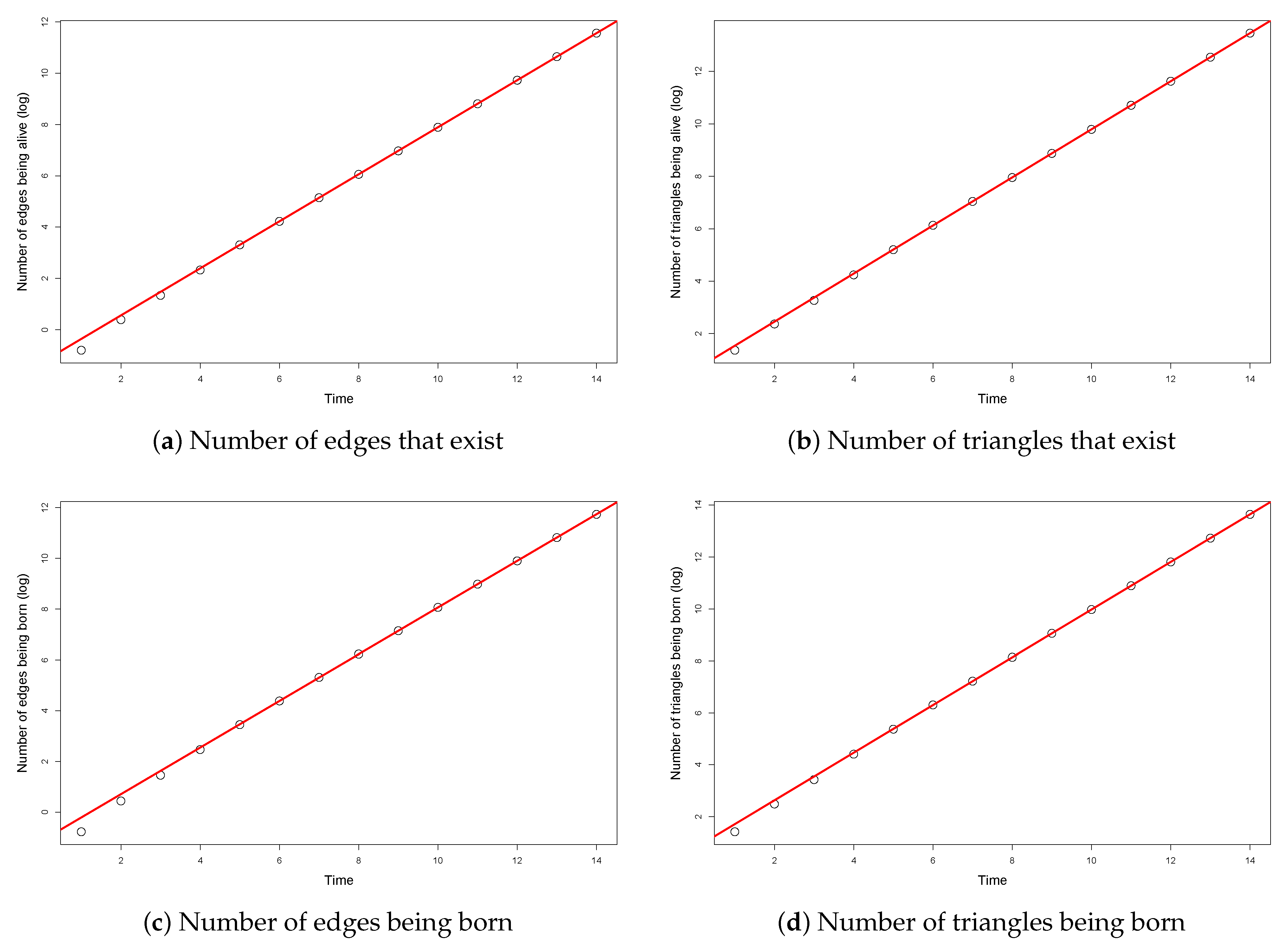
According to Theorem 2, for large t, the graphs of the numbers of edges and triangles are approximately straight lines on the logarithmic scale. To obtain empirical evidence of our Theorem 2, we investigated the slope of the simulated number of edges and triangles being born and being present up to time t on the logarithmic scale. The initial instability of the single processes (Figure 3) motivated us to exclude the first few observations from the calculations, but the lack of them was not relevant, because the asymptotic properties can be observed in the later stage of the processes.

For each parameter set, we stored the mentioned measurements only in integer time steps, and then we took the average of 100 simulated processes. In Figure 4, an example is shown for a specific parameter set ($r_1=0.1$, $p_1=0.2$, $p_3=0.6$, $b=0.25$, $c=0.25$). The values of the averages are plotted by dots. In each case, we fitted a regression line (plotted by continuous red line) to the last 9 values. We can see that the fit is perfect, thus, supporting our theorem.

Our main goal was to obtain a 95% confidence interval for the slope of the linear regression line, as that was our simulated approximation of the Malthusian parameter $\alpha$.

Table 1. The 95% confidence intervals for $\alpha$.

	${\mathit{r}}_1$	${\mathit{p}}_1$	${\mathit{p}}_2$	b	c	$\widehat{\mathit{\alpha }}$	2.5%	97.5%
E	0.1	0.5	0.5	0.2	0.4	0.5394	0.5393 *	0.5443 *
T							0.5390 *	0.5440 *
$\tilde{E}$							0.5410	0.5453
$\tilde{T}$							0.5395	0.5444
E	0.1	0.2	0.6	0.25	0.25	0.9133	0.9130 *	0.9141 *
T							0.9134	0.9142
$\tilde{E}$							0.9133 *	0.9141 *
$\tilde{T}$							0.9133 *	0.9148 *
E	0.1	0.2	0.6	0.45	0.35	0.6622	0.6585 *	0.6659 *
T							0.6606 *	0.6648 *
$\tilde{E}$							0.6608 *	0.6647 *
$\tilde{T}$							0.6597 *	0.6638 *

contains the boundaries of the 95% confidence intervals for $\alpha$. The columns labelled with $2.5\%$ and $97.5\%$ refer to the lower and the upper bounds obtained from simulations, while the column of $\widehat{\alpha }$ refers to the numerical solution of Equation (25).

For each fixed parameter set $\{r_1,p_1,p_2,b,c\}$, we present the confidence intervals calculated from the number of edges being born (E) resp. being present ($\tilde{E}$) and from the number of triangles being born (T) resp. being present ($\tilde{T}$) up to time $t=14$. The confidence intervals containing the numerical Malthusian parameter $\widehat{\alpha }$ are highlighted with the * symbol. We see that any confidence interval is narrow, and it either contains $\widehat{\alpha }$, or $\widehat{\alpha }$ is very close to the interval. These results show that the approximation is good for moderate values of t.

Finally, we present some simulation results for Theorem 3, that is, for the probability of extinction of the evolution process. We made the following computer experiment for any fixed parameter set $\{r_1,p_1,p_2,b,c\}$ and for type 2 and type 3 ancestors. We started to generate the process. If this process reached $2^{10}$ birth steps, then we stopped it and considered it as a non-extinct process. Otherwise, when the process did not reach $2^{10}$ birth steps, then the process died out. Applying the above method, we generated ${10}^5$ processes for each parameter sets and counted the relative frequencies of the processes being extinct.

In

Table 2. Comparison of the numeric values of the extinction probabilities and their relative frequencies from ${10}^5$ repetitions.

${\mathit{r}}_1$	${\mathit{p}}_1$	${\mathit{p}}_2$	b	c	Ancestor	Numeric	Simulation
0.1	0.2	0.6	0.8	0.8	2	0.9095	0.9053
					3	0.8855	0.8805
0.2	0.3	0.6	0.7	0.7	2	0.9247	0.9184
					3	0.9141	0.9070
0.3	0.3	0.5	0.6	0.6	2	0.7371	0.7207
					3	0.6896	0.6834

, we show some of the results. Column Ancestor contains the type of the ancestor. In the column Numeric we show the numeric solution of the non-linear equation in Theorem 3. We used Julia’s trust region method. Column Simulation contains the relative frequencies extracted from the simulations. The simulation results slightly underestimate the numeric values. This is reasonable because we stopped all processes at a fixed time.

8. Basic Facts on Branching Processes

In our paper, we use known results of the theory of continuous-time branching processes. The single type general Crump–Mode–Jagers branching processes have been described e.g., in [21,22,23]. The general multi-type branching processes have been studied, e.g., in [11,19,24].

Here, we give a short description of the general multi-type branching processes based on [11]. The individuals of this process can be of p different types, which we denote by $1,2,\dots ,p$. Any individual x is described by the quantities ${\lambda }_x,{\xi }_x,{\Phi }_x,{\Psi }_x,\dots$. The quantities ${\lambda }_x,{\xi }_x,{\Phi }_x,{\Psi }_x,\dots$ are independent copies of the quantities $\lambda ,\xi ,\Phi ,\Psi ,\dots$. Thus, we should give the definition of $\lambda ,\xi ,\Phi ,\Psi ,\dots$, which we consider as the quantities corresponding to the generic individual.

The lifetime $\lambda$ is a non-negative random variable which is not necessarily independent from the reproduction. The lifetime distribution is $L\left(t\right)=\mathbb{P}\left(\lambda \le t\right)$. The reproduction process is ${\xi }_i\left(t\right)=\left({\xi }_{i,1}\left(t\right),\dots ,{\xi }_{i,p}\left(t\right)\right)$, $t\ge 0$. Here, the random point process ${\xi }_{i,j}$ describes the births of type j offspring of a type i mother. ${\xi }_{i,j}\left(t\right)$ gives the number of type j offspring of a type i mother up to time t. ${\xi }_{i,j}$ is determined by the birth events and the numbers of offspring. The process starts at time $t=0$ with one individual called the ancestor and denoted by $x_0$. When a child is born, it starts its own reproduction process and so on. The birth time of the individual x is denoted by ${\sigma }_x$.

Let $\Phi \left(t\right)$ be a non-negative random function that describes a certain aspect of the life history of the individual. It is usually assumed that $\Phi \left(t\right)=0$ for $t\le 0$. Then, $\Phi \left(t\right)$ is called a random characteristic. Let $\Psi \left(t\right)$ be another random characteristic. Thus, the behaviour of the individual x is described by ${\xi }_x,{\lambda }_x,{\Phi }_x,{\Psi }_x,\dots$.

Let us define the branching process ${}_{x_0}{Z}^{\Phi }\left(t\right)$ counted by the characteristic $\Phi$ as

$${}_{x_0}{Z}^{\Phi }\left(t\right)=\sum _x{\Phi }_x\left(t-{}_{x_0}{\sigma }_x\right),$$

where we summarize for all individuals x. Here, the left subscript $x_0$ of Z and of the birth time ${\sigma }_x$ is important, because it denotes that the process starts with ancestor $x_0$ and the type of $x_0$ has influence for the evolution of the population.

Let us denote by $m_{i,j}\left(t\right)$ the reproduction function, which is the expected reproduction number $m_{i,j}\left(t\right)=\mathbb{E}{\xi }_{i,j}\left(t\right)$.

The following facts are well-known (see [11] or [24]).

We assume the following basic conditions in this section.

(a) Not all of the measures $m_{i,j}$ are concentrated on a lattice.

Let

$$m_{i,j}^{\ast }\left(\kappa \right)={\int }_0^{\infty }{e}^{-\kappa t}{m}_{i,j}\left(dt\right),i,j=1,\dots ,p,$$

be the Laplace transform of $m_{i,j}$. Let $M\left(\kappa \right)$ be the matrix

$$M\left(\kappa \right)={\left(m_{i,j}^{\ast }\left(\kappa \right)\right)}_{i,j=1}^p.$$

(b1) There exists a positive Malthusian parameter $\alpha$ that is a finite positive value so that $M\left(\alpha \right)$ has finite entries only, and the Perron–Frobenius root of $M\left(\alpha \right)$ is equal to 1. Here, the Perron–Frobenius root is the largest eigenvalue of the matrix. Let ${(v_1,\dots ,v_p)}^{\top }$ be the right positive eigenvector and ${(u_1,\dots ,u_p)}^{\top }$ the left positive eigenvector of $M\left(\alpha \right)$ corresponding to the Perron–Frobenius root. We normalize them as ${\sum }_{i=1}^p{v}_i=1$ and ${\sum }_{i=1}^p{u}_i{v}_i=1$.

(b2) The matrix ${\left(m_{i,j}(\infty )\right)}_{i,j=1}^p$ has an infinite entry, or all of them are finite, and its Perron–Frobenius root is greater than 1.

(c) The first moment of $e^{-\alpha t}{m}_{i,j}\left(dt\right)$ is finite and positive; that is,

$$0<{\int }_0^{\infty }t{e}^{-\alpha t}{m}_{i,j}\left(dt\right)<\infty ,i,j=1,\dots ,p.$$

(d) There exists a finite positive integer K so that all elements of the Kth power of the matrix ${\left(m_{i,j}\left(\infty \right)\right)}_{i,j=1}^p$ are positive.

Let

$${}_{\alpha }{\xi }_{i,j}(\infty )={\int }_0^{\infty }{e}^{-\alpha t}{\xi }_{i,j}\left(dt\right).$$

(68)

Proposition 4.

Let α be the Malthusian parameter. Assume that the random characteristic Φ satisfies the following conditions:

(i) 

$\Phi \left(t\right)\ge 0$,

(ii) 

The trajectories of Φ belong to the Skorohod space D, i.e., they do not have discontinuities of the second kind,

(iii) 

$\mathbb{E}\left({sup}_t\Phi \left(t\right)\right)<\infty$.

Assume also

(iv) 

for some $\epsilon >0$

$${\int }_0^{\infty }t{(log(1+t))}^{1+\epsilon }{e}^{-\alpha t}{m}_{i,j}\left(dt\right)<\infty ,i,j=1,\dots ,p$$

and

(v) 

for some $\epsilon >0$

$$\mathbb{E}\underset{t\ge 0}{sup}\left\{max\left\{t{(log(1+t))}^{1+\epsilon },1\right\}{e}^{-\alpha t}\Phi \left(t\right)\right\}<\infty$$

for any ancestor.

Then,

$$\underset{t\to \infty }{lim}{e}^{-\alpha t}{}_{x_0}{Z}^{\Phi }\left(t\right)={}_{x_0}{Y}_{\infty }{v}_i{m}_{\infty }^{\Phi }$$

(69)

is likely, where i is the type of $x_0$,

$$m_{\infty }^{\Phi }={\displaystyle \frac{{\sum }_{j=1}^p{u}_j{\int }_0^{\infty }{e}^{-\alpha t}\mathbb{E}{\Phi }_j\left(t\right)dt}{{\sum }_{l,j=1}^p{u}_l{v}_j{\int }_0^{\infty }t{e}^{-\alpha t}{m}_{l,j}\left(dt\right)}},$$

(70)

${}_{x_0}{Y}_{\infty }$ is an a.s. non-negative random variable depending on the type of the ancestor $x_0$ but not depending on the choice of Φ.

If, in addition, we assume that

(vi) 

$$\mathbb{E}\left[{}_{\alpha }{\xi }_{i,j}(\infty ){log}^{+}{}_{\alpha }{\xi }_{i,j}(\infty )\right]<\infty ,i,j=1,\dots ,p,$$

(71)

then $\mathbb{E}\left({}_{x_0}{Y}_{\infty }\right)=1$, ${}_{x_0}{Y}_{\infty }$ is positive with positive probability, and ${}_{x_0}{Y}_{\infty }$ is a.s. positive on the survival set.

The proof is a simple consequence of Theorem 2.4 and Proposition 4.1 of [11].

9. Discussion

In this paper, a new network evolution model was introduced. This model was inspired by those networks where small substructures play important role. In social life, such substructures could be a group of friends. In the theory of networks, these substructures are called motifs. In this paper, for the sake of simplicity, we consider only two types of substructures, the edges and the triangles. The novelty of the paper is the usage of a two-type continuous time branching process to describe these two types of interactions. Thus, despite [7,10], the theory of multi-type branching processes was applied for certain substructures of the network and not just for the nodes. Our paper extends the former studies of [16,17], where only one type of interaction was considered.

In this paper, we proved that the magnitude of the number of triangles on the event of non-extinction is $e^{\alpha t}$, where $\alpha$ is the Malthusian parameter. We obtained similar results for the number of edges. We also studied the degree process of a fixed vertex and the probability of the extinction. Our results are similar to the ones obtained for the simpler models in [16,17]. In addition to mathematical proofs, the results were illustrated by simulations.

In future extensions of the model, more than two types of substructures can be studied using the theory of multi-type branching processes.