Nonstandard Finite Difference Schemes for an SIR Epidemic Model

Abstract

This paper aims to present two nonstandard finite difference (NFSD) methods to solve an SIR epidemic model. The proposed methods have important properties such as positivity and boundedness and they also preserve conservation law. Numerical comparisons confirm that the accuracy of our method is better than that of other existing standard methods such as the second-order Runge–Kutta (RK2) method, the Euler method and some ready-made MATLAB codes.

1. Introduction

The modeling of physical, chemical, and biological systems is commonly based on nonlinear ordinary differential equations (ODEs). Mathematical models and their simulations are important for understanding the quality and quantity of these systems. Numerical methods, such as Euler and Runge–Kutta methods for solving the mentioned equations, are typically used [1,2,3,4,5,6,7,8,9,10,11,12]. A downside of these methods is that the qualitative characteristics of a true solution are not transferred to the numerical solution. To overcome such a deficiency, the NSFD methods were introduced by Mickens [13,14]. Indeed, these methods were proposed in order to preserve the main characteristics of systems of differential equations, which preserve positivity, boundedness, stability of equilibrium points and conservation law [15,16,17,18,19,20,21,22,23,24,25,26,27,28,29,30,31,32,33,34,35,36,37,38,39,40,41]. For a method to be designated as an NSFD, at least one of the following criteria should be fulfilled:

•

In the first-order discrete derivatives, step-size h in the denominator is replaced by a function $\varphi \left(h\right)$, such that

$$\varphi \left(h\right)=h+\mathcal{O}\left(h^2\right),\mathrm{as}h\to 0.$$

(1)

•

Nonlinear terms in $f\left(y\right)$ can be approximated non-locally (by a suitable function of several of the mesh points), for instance:

$$x^2\approx x_{k+1}{x}_k,x^3\approx x_{k+1}{x}_k^2,x(1-x)\approx x_k(1-x_{k+1}).$$

The main goal of this article is to introduce and present two NSFD methods to solve an SIR epidemic model. The constructed methods preserve the characteristics of the mathematical model such as positivity, boundedness, stability of equilibrium points and conservation law. The rest of the paper is structured as follows: In Section 2, we introduce the mathematical model for the SIR epidemic model with its equilibrium points. We also investigate the positivity properties of the model. In Section 3, the new schemes are proposed. The positivity property is investigated in Section 4. In Section 5, we investigate the elementary stability of the new schemes. In Section 6, we present the results obtained by the new schemes and some schemes such as the Euler method, ode45 (a MATLAB’s standard solver for ODEs ), and so on.

2. Mathematical Model

Here, the mathematical model of the SIR epidemic introduced in [36] is presented. This model consists of the following three characteristics:

•

$S\left(t\right)$: susceptible individuals;

•

$I\left(t\right)$: infective individuals;

•

$R\left(t\right)$: recovered individuals.

The mathematical model of the SIR epidemic presented in [42] is related to rubella disease in London. The model is introduced by a nonlinear differential equation system as follows:

$$\begin{array}{cc}\hfill & S^{\prime }\left(t\right)=N\mu -\mu S\left(t\right)-N\beta \frac{S\left(t\right)I\left(t\right)}{1+aI},\hfill \\ \hfill & I^{\prime }\left(t\right)=N\beta \frac{S\left(t\right)I\left(t\right)}{1+aI}-(\mu +\nu )I\left(t\right),\hfill \\ \hfill & R^{\prime }\left(t\right)=\nu I\left(t\right)-\mu R\left(t\right),\hfill \\ \hfill & S\left(0\right)=S_0,I\left(0\right)=I_0,R\left(0\right)=R_0,t>0,a>0,\hfill \end{array}$$

(2)

where

•

$\beta$: The transmission rate;

•

$\mu$: The death rate;

•

$\nu$: The recovery rate;

•

a: The inhibitory rate;

•

N: The total population size;

and they are all positive.

The consecutive system of equations, if added together, clearly satisfies conservation law, which implies that the population is constant. The population can be normalized to one, since it is assumed to be constant:

$$S\left(t\right)+I\left(t\right)+R\left(t\right)=1.$$

The above equation must be valid for any numerical method. The reproduction number of system (2) is as follows:

$${\mathcal{R}}_0=\frac{N\beta }{(\mu +\nu )},$$

the system (2) has two equilibrium points as follows:

• $E_0^{*}=(1,0,0)$: the disease-free equilibrium;
• $E^{*}=(S^{*},I^{*},R^{*})$: the endemic equilibrium,

where

$$E^{*}=(S^{*},I^{*},R^{*})=\left(\frac{{\mathcal{R}}_0\mu a+N\beta }{{\mathcal{R}}_0(\mu a+N\beta )},\frac{\mu ({\mathcal{R}}_0-1)}{\mu a+N\beta },\frac{\nu ({\mathcal{R}}_0-1)}{\mu a+N\beta }\right).$$

3. Construction of New Schemes

In this section, we propose a family of NSFD schemes for the system (2) in the following form:

$$\begin{array}{cc}\hfill & {\displaystyle \frac{S^{n+1}-S^n}{\psi \left(h\right)}}=\mu -\mu (\gamma S^{n+1}+\delta S^n)-N\beta (\eta S^{n+1}+\theta S^n)\frac{I^n}{1+a{I}^n},\hfill \\ \hfill & {\displaystyle \frac{I^{n+1}-I^n}{\psi \left(h\right)}}=N\beta (\eta S^{n+1}+\theta S^n)\frac{I^n}{1+a{I}^n}-\mu (\gamma I^{n+1}+\delta I^n)-\nu (\eta I^{n+1}+\theta I^n),\hfill \\ \hfill & {\displaystyle \frac{R^{n+1}-R^n}{\psi \left(h\right)}}=\nu (\eta I^{n+1}+\theta I^n)-\mu (\gamma R^{n+1}+\delta R^n),\hfill \end{array}$$

(3)

with $\gamma +\delta =1$, $\eta +\theta =1$ and

$$\psi \left(h\right)=\frac{exp\left(\mu h\right)-1}{\mu },\psi \left(h\right)=h+O\left(h^2\right).$$

Note that this scheme satisfies $R^{\prime }\left(t\right)+S^{\prime }\left(t\right)+I^{\prime }\left(t\right)=0$, as $n\to \infty$. In addition, it follows from (3) that

$$S^{n+1}+R^{n+1}+I^{n+1}=\frac{\mu \psi \left(h\right)+(1-\mu \delta \psi \left(h\right))(S^n+R^n+I^n)}{1+\mu \gamma \psi \left(h\right)}.$$

Thus, if $S^n+R^n+I^n=1$ for all $n\ge 1$ and, since, $\gamma =1-\delta$ then $S^{n+1}+R^{n+1}+I^{n+1}=1$ for all $n\ge 1$. Therefore, the conservation law property holds.

We have chosen two different formulas of (3), given as follows:

3.1. Scheme 1

Formula (4) is obtained by taking $\gamma =1$, $\delta =0$, $\eta =1$, $\theta =0$:

$$\begin{array}{cc}\hfill & S^{n+1}={\displaystyle \frac{\psi \left(h\right)\mu +S^n}{1+\psi \left(h\right)\mu +\frac{\psi \left(h\right)N\beta I^n}{1+a{I}^n}}}=F(S^n,I^n),\hfill \\ \hfill \\ \hfill & I^{n+1}={\displaystyle \frac{\left(1+\frac{\psi \left(h\right)N\beta }{1+a{I}^n}F(S^n,I^n)\right)I^n}{1+(\mu +\nu )\psi \left(h\right)}}=G(S^n,I^n),\hfill \\ \hfill \\ \hfill & R^{n+1}=1-S^{n+1}-I^{n+1}={\displaystyle \frac{\psi \left(h\right)\nu I^{n+1}+R^n}{\psi \left(h\right)\mu }}.\hfill \end{array}$$

(4)

3.2. Scheme 2

Formula (5) is obtained by taking $\gamma =2$, $\delta =-1$, $\eta =1$, $\theta =0$:

$$\begin{array}{cc}\hfill & S^{n+1}={\displaystyle \frac{\psi \left(h\right)\mu +S^n(1+\psi \left(h\right)\mu )}{1+2\psi \left(h\right)\mu +\psi \left(h\right)N\beta \frac{I^n}{1+a{I}^n}}}=\overline{F}(S^n,I^n),\hfill \\ \hfill \\ \hfill & I^{n+1}={\displaystyle \frac{\left(1+\mu \psi \left(h\right)+\frac{N\beta \psi \left(h\right)}{1+a{I}^n}\overline{F}(S^n,I^n)\right)I^n}{1+2\psi \left(h\right)\mu +\nu \psi \left(h\right)}}=\overline{G}(S^n,I^n),\hfill \\ \hfill \\ \hfill & R^{n+1}=1-S^{n+1}-I^{n+1}=\frac{(1+\mu )R^n+\nu \psi \left(h\right)I^{n+1}}{2\mu \psi \left(h\right)}.\hfill \end{array}$$

(5)

4. Positivity

In this section, the positive property of the proposed methods in the previous section is investigated. Positivity means that the non-negativity of initial data is preserved over time in the approximate solution. It should be noted that the positive property of a numerical method used to solve differential models related to population biology is very important because the variables used in the subpopulation models can never be negative values (see, for example, [43]).

Definition 1.

A finite difference method is positive if

$$\forall h>0\left(\mathit{stepsize}\right),\mathit{and}{y}_0\in {\mathbb{R}}^{+}\left(\mathit{initialcondition}\right),$$

the other solutions are also positive, that is, we have $y_k\in {\mathcal{R}}^{+}$ for any $k\in \mathbb{N}$.

Theorem 1.

Equations (4) and (5) are positive.

Proof. 

Since the parameters B, N, ν, a and μ are positive, then the numerical schemes (4) and (5) represent positive NSFD methods for any $\psi \left(h\right)>0$ when the initial values $S\left(0\right)$, $I\left(0\right)$ and $R\left(0\right)$ are non-negative. □

5. Elementary Stability

In this section, the stability properties of the proposed methods are investigated and sufficient conditions to preserve this property of the equilibrium points of model (2) are proposed. The finitedifference methods that have this stability property are called elementary stable methods [44].

Definition 2.

The finite difference method is called elementary stable, if for any value of the step size h, its only equilibrium points $\overline{E}$ are those of the original differential system, the linear stability properties of each $\overline{E}$ being the same for both the differential system and the discrete method.

Lemma 1.

For the quadratic equation ${\lambda }^2-\Lambda \lambda +\omega =0$, by using the well-known Jury condition, both roots satisfy $|{\lambda }_i|<1,i=1,2$ if the following conditions are satisfied:

• $1+\Lambda +\omega >0$,
• $1-\Lambda +\omega >0$,
• $\omega <1$.

Theorem 2.

Equations (4) and (5) are elementary stables.

Proof. 

In order to examine the convergence of schemes (4) and (5), it is enough to only consider the first and second equations of (4) and (5). The equilibrium points of (4) are exactly the equilibria $E_0^{*}$ and $E^{*}$ of system (2). The Jacobian J of the Equation (4) has the form $J(S^n,I^n)=\left[\begin{array}{cc}\frac{\partial F}{\partial S}& \frac{\partial F}{\partial I}\\ & \\ \frac{\partial G}{\partial S}& \frac{\partial G}{\partial I}\end{array}\right]$,

$$\begin{array}{cc}\hfill & {\displaystyle \frac{\partial F}{\partial S}}={\displaystyle \frac{1}{1+\psi \left(h\right)(\mu +\frac{N\beta I^n}{1+a{I}^n})}}\hfill \\ \\ \hfill & {\displaystyle \frac{\partial F}{\partial I}}=-\left[{\displaystyle \frac{1}{{\left(1+\psi \left(h\right)\left(\mu +\frac{N\beta I^n}{1+a{I}^n}\right)\right)}^2}}\right]\left((S^n+\mu \psi \left(h\right))(\frac{N\beta \psi \left(h\right)}{1+a{I}^n}-\frac{aN\beta \psi \left(h\right)I^n}{{(1+I^n)}^2})\right),\hfill \\ \\ \hfill & {\displaystyle \frac{\partial G}{\partial S}}=\left({\displaystyle \frac{1}{1+(\mu +\nu )\psi \left(h\right)}}\right)\left({\displaystyle \frac{N\beta \psi \left(h\right)I^n}{1+a{I}^n}}\right)\left({\displaystyle \frac{\partial F}{\partial S}}\right)\hfill \\ \hfill & =\left({\displaystyle \frac{1}{1+(\mu +\nu )\psi \left(h\right)}}\right)\left({\displaystyle \frac{N\beta \psi \left(h\right)I^n}{1+a{I}^n}}\right)\left({\displaystyle \frac{1}{1+\psi \left(h\right)(\mu +\frac{N\beta I^n}{1+a{I}^n})}}\right)\hfill \\ \\ \hfill & {\displaystyle \frac{\partial G}{\partial I}}=\left({\displaystyle \frac{1}{1+(\mu +\nu )\psi \left(h\right)}}\right)\left[1+{\displaystyle \frac{N\beta \psi \left(h\right)}{1+a{I}^n}}F(s^n,I^n)+{\displaystyle \frac{N\beta \psi \left(h\right)I^n}{1+a{I}^n}}\left({\displaystyle \frac{\partial F}{\partial I}}\right)-\frac{aN\beta \psi \left(h\right)I^{n}F}{{(1+a{I}^n)}^2}\right],\hfill \\ \\ \hfill & =\left({\displaystyle \frac{1}{1+(\mu +\nu )\psi \left(h\right)}}\right)[1+{\displaystyle \frac{N\beta \psi \left(h\right)}{1+a{I}^n}}\left({\displaystyle \frac{\psi \left(h\right)\mu +S^n}{1+\psi \left(h\right)\mu +\frac{\psi \left(h\right)N\beta I^n}{1+a{I}^n}}}\right)\hfill \\ \\ \hfill & +{\displaystyle \frac{N\beta \psi \left(h\right)I^n}{1+a{I}^n}}(-\left[{\displaystyle \frac{1}{{\left(1+\psi \left(h\right)\left(\mu +\frac{N\beta I^n}{1+a{I}^n}\right)\right)}^2}}\right]\left((S^n+\mu \psi \left(h\right))(\frac{N\beta \psi \left(h\right)}{1+a{I}^n}-\frac{aN\beta \psi \left(h\right)I^n}{{(1+I^n)}^2})\right))\hfill \\ \hfill & -\frac{aN\beta \psi \left(h\right)I^n}{{(1+a{I}^n)}^2}\left({\displaystyle \frac{\psi \left(h\right)\mu +S^n}{1+\psi \left(h\right)\mu +\frac{\psi \left(h\right)N\beta I^n}{1+a{I}^n}}}\right)],\hfill \end{array}$$

substituting $E_0^{*}$ in $J(S^n,I^n)$ we obtain

$$\begin{array}{c}\hfill J\left(E_0^{*}\right)=\left(\begin{array}{cc}{\displaystyle \frac{1}{1+\psi \left(h\right)\mu }}& -{\displaystyle \frac{NB\psi \left(h\right)}{1+\psi \left(h\right)\mu }}\\ \\ 0& {\displaystyle \frac{1+NB\psi \left(h\right)}{1+(\mu +\nu )\psi \left(h\right)}},\end{array}\right),\end{array}$$

from which

$$\begin{array}{c}\hfill {\lambda }_1={\displaystyle \frac{1}{1+\psi \left(h\right)\mu }},{\lambda }_2={\displaystyle \frac{1+N\beta \psi \left(h\right)}{1+(\mu +\nu )\psi \left(h\right)}};\end{array}$$

therefore, it is obvious that $|{\lambda }_1|<1$ always holds and if ${\mathcal{R}}_0<1$, that is, $NB<\mu +\nu$, then $|{\lambda }_2|<1$. Hence, the disease equilibrium is asymptotically stable if ${\mathcal{R}}_0<1$ and otherwise it will be unstable.

If ${\mathcal{R}}_0>1$ system (2) has an endemic equilibrium point.

The Jacobian matrix of Equation (4) evaluated at the endemic equilibrium is

$$\begin{array}{c}\hfill J\left(E^{*}\right)=\left(\begin{array}{cc}\frac{1}{b}& -\frac{(c-d)}{b^2}\\ & \\ \frac{e}{fb}& \frac{1}{f}\left(1+(c-d)(\frac{1}{b}-\frac{e}{b^2})\right)\end{array}\right),\end{array}$$

where

$$\begin{array}{cc}\hfill & b=1+\psi \left(h\right)(\mu +\frac{NB{I}^{*}}{1+a{I}^{*}})>1,\hfill \\ \\ \hfill & c=(S^{*}+\mu \psi \left(h\right))\frac{NB\psi \left(h\right)}{1+a{I}^{*}}>0,\hfill \\ \\ \hfill & d=(S^{*}+\mu \psi \left(h\right))\frac{aNB\psi \left(h\right)I^{*}}{{(1+a{I}^{*})}^2}>0,\hfill \\ \\ \hfill & f=1+(\mu +\nu )\psi \left(h\right)>1\hfill \\ \\ \hfill & e=\frac{NB\psi \left(h\right)I^{*}}{1+a{I}^{*}}=\frac{NB\mu \psi \left(h\right)({\mathcal{R}}_0-1)}{{\mathcal{R}}_0\mu a+NB}>0.\hfill \end{array}$$

Eigenvalues of $J\left(E^{*}\right)$ are roots of the quadratic equation ${\lambda }^2-\Lambda \lambda +\omega =0$

$$\Lambda =TraceJ\left(E^{*}\right)=\frac{bf+b^2+(c-d)(b-e)}{b^{2}f}>0$$

since $c>d$ and $b>e$ and, also,

$$\omega =DetJ\left(E^{*}\right)=\frac{b^2+(c-d)(b-e)}{b^{3}f}+\frac{e(c-d)}{b^{3}f}=\frac{b^2+(c-d)b}{b^{3}f}>0.$$

Therefore, the equilibrium $E^{*}$ is stable if and only if all conditions of Lemma 1 hold. Since Λ and ω are positive, we have

$$\begin{array}{c}\hfill 1+\Lambda +\omega >0.\end{array}$$

(6)

Since $\frac{1}{b}<1$ and

$$\frac{1}{f}(1+\frac{(c-d)(b-e)}{b^2})<\frac{1}{f}(1+\frac{c-d}{b})<\frac{1}{f}(1+\frac{c}{b})<1$$

we have

$$\begin{array}{c}\hfill 1-\Lambda +\omega =(1-\frac{1}{b})\left(1-\frac{1}{f}(1+\frac{(c-d)(b-e)}{b^2})\right)+\frac{e(c-d)}{b^{3}f}>0;\end{array}$$

(7)

also,

$$\begin{array}{cc}\hfill \omega & =\frac{1}{bf}+\frac{c-d}{b^{2}f}<\frac{1}{bf}+\frac{c}{b^{2}f}<\frac{1}{bf}+\frac{c}{bf}=\frac{1+c}{bf}<1.\hfill \end{array}$$

(8)

From (6)–(8) we see that the conditions of Lemma 1 hold. Thus, when ${\mathcal{R}}_0>1$, the eigenvalues of $J\left(E^{*}\right)$ are less than the unity in the modulus, regardless of the size of h. Therefore dynamic consistence between the system (2) and Equation (4) is held around all equilibria, which leads to the elementary stability of (4).

Similarly, the equilibrium points of (5) are the same equilibria of the original system. The Jacobian J of (5) has the form $J(S^n,I^n)=\left[\begin{array}{cc}\frac{\partial \overline{F}}{\partial S}& \frac{\partial \overline{F}}{\partial I}\\ & \\ \frac{\partial \overline{G}}{\partial S}& \frac{\partial \overline{G}}{\partial I}\end{array}\right]$, where

$$\begin{array}{cc}\hfill & {\displaystyle \frac{\partial \overline{F}}{\partial S}}={\displaystyle \frac{1+\psi \left(h\right)\mu }{1+2\psi \left(h\right)\mu +\psi \left(h\right)NB\frac{I^n}{1+a{I}^n}}}\hfill \\ \\ \hfill & {\displaystyle \frac{\partial \overline{F}}{\partial I}}=-\left[{\displaystyle \frac{1}{{\left(1+\psi \left(h\right)\left(2\mu +\frac{NB{I}^n}{1+a{I}^n}\right)\right)}^2}}\right]\left(\left(S^n(1+\mu \psi \left(h\right))+\mu \psi \left(h\right)\right)\left(\frac{NB\psi \left(h\right)}{1+a{I}^n}-\frac{aNB\psi \left(h\right)I^n}{{(1+a{I}^n)}^2}\right)\right),\hfill \\ \\ \hfill & {\displaystyle \frac{\partial \overline{G}}{\partial S}}={\displaystyle \frac{NB\psi \left(h\right)\frac{I^n}{1+a{I}^n}{\displaystyle \frac{\partial \overline{F}}{\partial S}}}{1+2\psi \left(h\right)\mu +\nu \psi \left(h\right)}}={\displaystyle \frac{NB\psi \left(h\right)\frac{I^n}{1+a{I}^n}(1+\psi \left(h\right)\mu )}{(1+2\psi \left(h\right)\mu +\psi \left(h\right)NB\frac{I^n}{1+a{I}^n})(1+2\psi \left(h\right)\mu +\nu \psi \left(h\right))}}\hfill \\ \\ \hfill & {\displaystyle \frac{\partial \overline{G}}{\partial I}}=\left({\displaystyle \frac{1}{1+(2\mu +\nu )\psi \left(h\right)}}\right)\left[1+\mu \psi \left(h\right)+{\displaystyle \frac{NB\psi \left(h\right)}{1+a{I}^n}}\overline{F}(s^n,I^n)-{\displaystyle \frac{aNB\psi \left(h\right)I^n}{{(1+a{I}^n)}^n}}\overline{F}(s^n,I^n)+{\displaystyle \frac{NB\psi \left(h\right)I^n}{1+a{I}^n}}\left({\displaystyle \frac{\partial \overline{F}}{\partial I}}\right)\right],\hfill \\ \\ \hfill & =\left({\displaystyle \frac{1}{1+(2\mu +\nu )\psi \left(h\right)}}\right)[1+\mu \psi \left(h\right)+{\displaystyle \frac{NB\psi \left(h\right)}{1+a{I}^n}}\left({\displaystyle \frac{\psi \left(h\right)\mu +S^n(1+\mu \psi \left(h\right))}{1+2\psi \left(h\right)\mu +\frac{\psi \left(h\right)NB{I}^n}{1+a{I}^n}}}\right)\hfill \\ \\ \hfill & -{\displaystyle \frac{aNB\psi \left(h\right)I^n}{{(1+a{I}^n)}^2}}\left({\displaystyle \frac{\psi \left(h\right)\mu +S^n(1+\mu \psi \left(h\right))}{1+2\psi \left(h\right)\mu +\frac{\psi \left(h\right)NB{I}^n}{1+a{I}^n}}}\right)\hfill \\ \\ \hfill & +{\displaystyle \frac{NB\psi \left(h\right)I^n}{1+a{I}^n}}\left(-\left[{\displaystyle \frac{1}{{\left(1+\psi \left(h\right)\left(2\mu +\frac{NB{I}^n}{1+a{I}^n}\right)\right)}^2}}\right]\left(\left(S^n(1+\mu \psi \left(h\right))+\mu \psi \left(h\right)\right)\left(\frac{NB\psi \left(h\right)}{1+a{I}^n}-\frac{aNB\psi \left(h\right)I^n}{{(1+a{I}^n)}^2}\right)\right).\right]\hfill \end{array}$$

Substituting $E_0^{*}$ in $J(S^n,I^n)$, we obtain

$$\begin{array}{c}\hfill J\left(E_0^{*}\right)=\left(\begin{array}{cc}{\displaystyle \frac{1+\psi \left(h\right)\mu }{1+2\psi \left(h\right)\mu }}& {\displaystyle \frac{-NB\psi \left(h\right)}{1+2\psi \left(h\right)\mu }}\\ \\ 0& {\displaystyle \frac{1+\psi \left(h\right)\mu +NB\psi \left(h\right)}{1+2\psi \left(h\right)\mu +\psi \left(h\right)\nu }}\end{array}\right),\end{array}$$

from which

$$\begin{array}{c}\hfill {\lambda }_1={\displaystyle \frac{1+\psi \left(h\right)\mu }{1+2\psi \left(h\right)\mu }},{\lambda }_2={\displaystyle \frac{1+\psi \left(h\right)\mu +NB\psi \left(h\right)}{1+2\psi \left(h\right)\mu +\psi \left(h\right)\nu }}.\end{array}$$

Therefore, it is clear that $|{\lambda }_1|<1$ always holds and if ${\mathcal{R}}_0<1$, that is, $NB<\mu +\nu$, then $|{\lambda }_2|<1$. Hence, the disease equilibrium is asymptotically stable if ${\mathcal{R}}_0<1$; otherwise, it will be unstable.

If ${\mathcal{R}}_0>1$, system (2) has an endemic equilibrium point.

The Jacobian matrix of Equation (5) evaluated at the endemic equilibrium is

$$\begin{array}{c}\hfill J\left(E^{*}\right)=\left(\begin{array}{cc}\frac{g}{b}& -\frac{c-d}{b^2}\\ & \\ \frac{eg}{bf}& \frac{1}{f}(g+(c-d)(\frac{1}{b}-\frac{e}{b^2}))\end{array}\right),\end{array}$$

where

$$\begin{array}{cc}\hfill & g=1+\psi \left(h\right)\mu >1,\hfill \\ \\ \hfill & b=1+2\psi \left(h\right)\mu +NB\psi \left(h\right)\frac{I^{*}}{1+a{I}^{*}}>1,\hfill \\ \\ \hfill & c=\frac{NB\psi \left(h\right)}{1+a{I}^{*}}\left(\psi \left(h\right)\mu +S^{*}(1+\psi \left(h\right)\mu )\right)>0\hfill \\ \\ \hfill & d=\frac{aNB\psi \left(h\right)I^{*}}{{(1+a{I}^{*})}^2}\left(\psi \left(h\right)\mu +S^{*}(1+\psi \left(h\right)\mu )\right)>0\hfill \\ \\ \hfill & f=1+2\psi \left(h\right)\mu +\psi \left(h\right)\nu >1\hfill \\ \\ \hfill & e=NB\psi \left(h\right)\frac{I^{*}}{1+a{I}^{*}}>0.\hfill \end{array}$$

Eigenvalues of $J\left(E^{*}\right)$ are roots of the quadratic equation ${\lambda }^2-\Lambda \lambda +\omega =0$, where

$$\Lambda =TraceJ\left(E^{*}\right)=\frac{gbf+g{b}^2+(c-d)(b-e)}{f{b}^2}>0$$

since $c-d>0$ and $b-e>0$, and also,

$$\omega =DetJ\left(E^{*}\right)=\frac{b^2{g}^2+g(c-d)(b-e)}{b^{3}f}+\frac{(c-d)eg}{b^{3}f}=\frac{g^2{b}^2+(c-d)gb}{b^{3}f}>0.$$

Therefore, the equilibrium $E^{*}$ is stable if and only if all conditions of Lemma 1 hold. Since Λ and ω are positive we have

$$\begin{array}{c}\hfill 1+\Lambda +\omega >0.\end{array}$$

(9)

Since $\frac{e}{b}<1$ and

$$\frac{1}{f}(g+\frac{(c-d)(b-e)}{b^2})<\frac{1}{f}(g+\frac{c}{b})=\frac{gb+c}{fb}<1$$

we have

$$\begin{array}{c}\hfill 1-\Lambda +\omega =(1-\frac{g}{b})\left(1-\frac{1}{f}(g+\frac{(c-d)(b-e)}{b^2})\right)+\frac{(c-d)eg}{b^{3}f}>0;\end{array}$$

(10)

also,

$$\begin{array}{cc}\hfill \omega & =\frac{g^2}{bf}+\frac{(c-d)g}{b^{2}f}<\frac{g^2}{bf}+\frac{cg}{bf}=\frac{g(g+c)}{bf}<1\hfill \end{array}$$

(11)

From (9)–(11), we see that the conditions of Lemma 1 holds. Then, the eigenvalues of $J\left(E^{*}\right)$ are less than the unity in the modulus, regardless of the size of h, when ${\mathcal{R}}_0>1$. Therefore dynamic consistence between the system (2) and Equation (5) is held around all equilibria, which leads to the elementary stability of (5). □

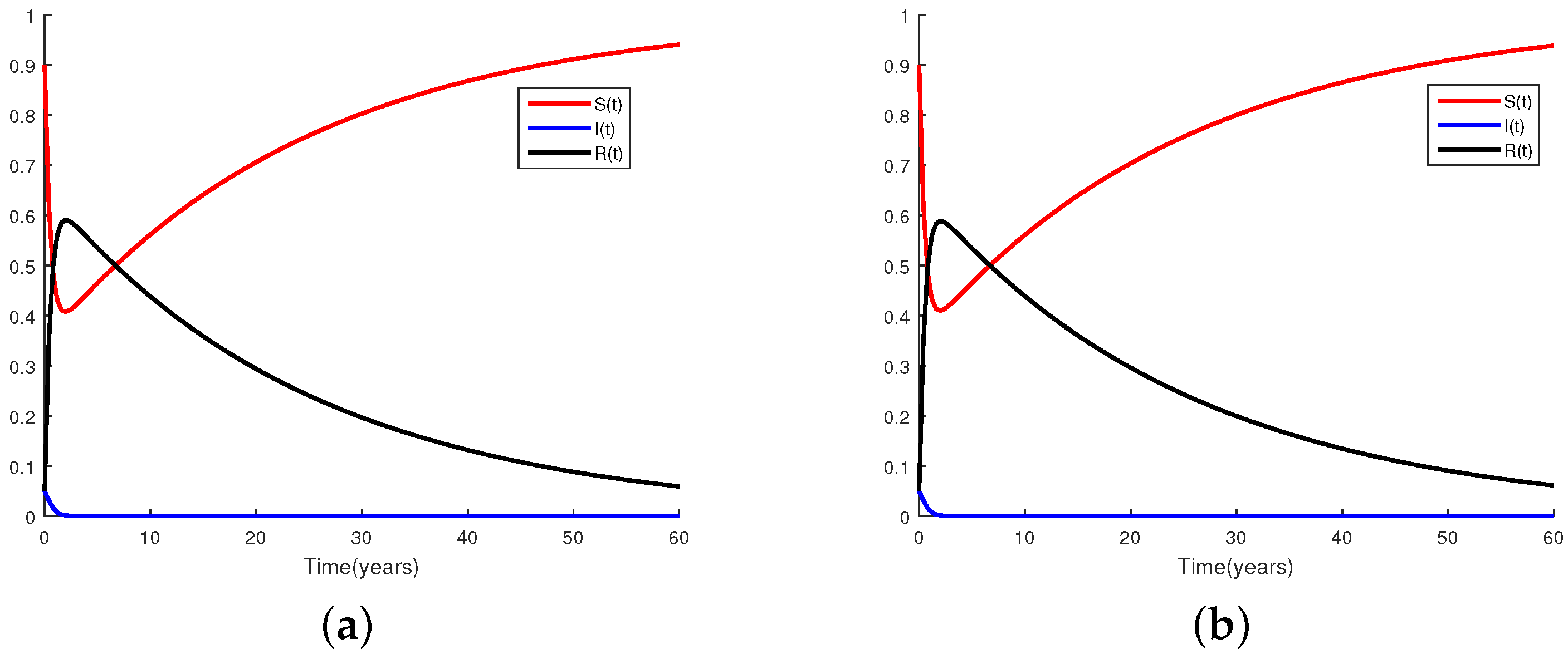
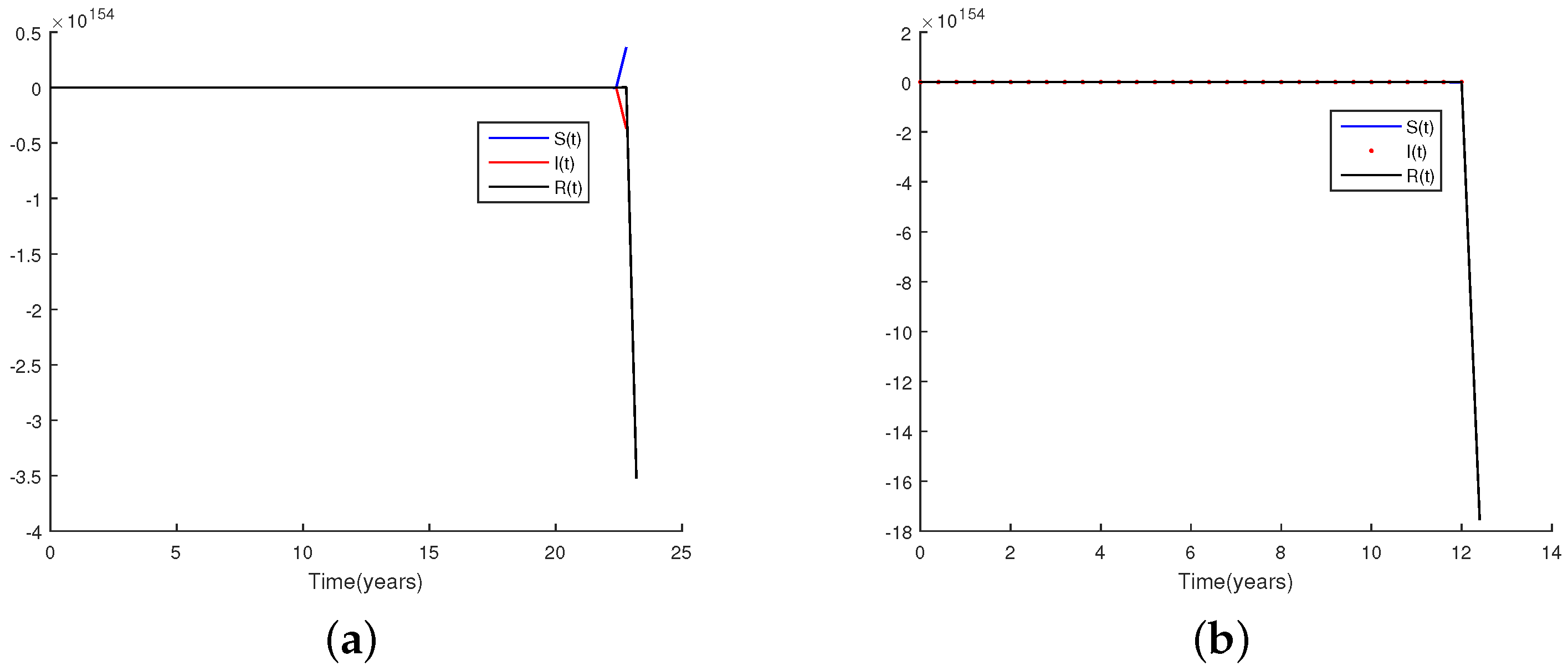
6. Numerical Results

In this section, we present some numerical results obtained by applying the new methods. These results indicate the efficiency of the methods. Consider model (2) with the parameters

$$\mu =0.04,\nu =24,NB=123.$$

The epidemic model (2) has a disease free equilibrium point for $R_0<1$ and an endemic equilibrium point for $R_0>1$. Figure 1 shows that, for ${\mathcal{R}}_0>1$, the new methods converge to the endemic equilibrium point and produce positive results for all times, while the ready-made MATLAB codes do not converge or sometimes produce negative values.

Figure 2 shows that the new schemes provide good approximations and converge to the endemic equilibrium. To see the influence of inhibitory constant (a), we show in Figure 3 and Figure 4 the numerical solutions of model (2) with $h=0.1$ and initial value $S\left(0\right)=0.9$, $I\left(0\right)=0.05$ and $R\left(0\right)=0.05$ using different values of a. It is shown that all numerical solutions obtained by the proposed NSFD schemes with $a=0.05,1,5,10$ are convergent to the EE point. It can be seen that NSFD schemes with a great inhibitory constant have better convergence to an endemic equilibrium point. In Figure 5 and Figure 6, we used the same parameters as above for $\mu$ and $\nu$, but we choose $NB=23$ so that ${\mathcal{R}}_0=0.9567$. As can be seen for each h, new schemes retain the positivity property, while the Euler method and the RK2 method give negative values when using the SIR model. It should be noted that, due to the very large numerical outputs at intervals larger than the range given in Figure 6, the system is unable to display those values.

7. Conclusions

In this work, two NSFD methods were proposed to solve the SIR pandemic model. The proposed model has two equilibrium points, which are dubbed disease free equilibrium points, that is, $E_0^{*}$, in which case ${\mathcal{R}}_0<1$, and the endemic equilibrium point $E^{*}$, wherein ${\mathcal{R}}_0>1$. It is shown that the proposed methods preserve features such as the positivity property, elementary stability and conservation law. By comparing the numerical results obtained from the new methods and the Runge–Kutta methods, it was shown that the NSFD numerical methods are made unconditionally stable by preserving conservation law for ${\mathcal{R}}_0<1$. They are also convergent to the disease-free equilibrium point for any step size. This behavior is also satisfied for ${\mathcal{R}}_0>1$. Moreover, the same behavior is obtained for ${\mathcal{R}}_0>1$. It is also confirmed that the ready-made MATLAB codes do not converge to the endemic equilibrium point. Therefore, it can be concluded that the new NSFD methods preserve features of the SIR epidemic model.

References

1. Arenasa, A.J.; Gonzlez-Parrab, G.; Chen-Charpentier, B.M. An Accurate Nonstandard Scheme of Predictor-Corrector Type for an SIR Epidemic Model, Technical Report 2009-01. Available online: https://citeseerx.ist.psu.edu/viewdoc/download?doi=10.1.1.407.848&rep=rep1&type=pdf (accessed on 27 April 2021).
2. Ashyralyev, A.; Agirseven, D.; Agarwal, R.P. Stability estimates for delay parabolic differential and difference equations. Appl. Comput. Math. 2020, 19, 175–204. [Google Scholar]
3. Ashyralyev, A.; Erdogan, A.S.; Tekalan, S.N. An investigation on finite difference method for the first order partial differential equation with the nonlocal boundary condition. Appl. Comput. Math. 2019, 18, 247–260. [Google Scholar]
4. Lin, C.; Hsu, C.-W.; Simos, T.E.; Tsitouras, C. Explicit, semi-symmetric, hybrid, six-step, eighth order methods for solving y″ = f(x, y). Appl. Comput. Math. 2019, 18, 296–304. [Google Scholar]
5. Lambert, J.D. Computational Methods in Ordinary Differential Equations; John Wiley & Sons/Wiley: Hoboken, NJ, USA, 1973. [Google Scholar]
6. Osa, A.L.; Olaoluwa, O.E. A Fifth-fourth Continuous Block Implicit Hybrid Method for the Solution of Third Order Initial Value Problems in Ordinary Differential Equations. Appl. Comput. Math. 2019, 8, 50–57. [Google Scholar]
7. Magagula, V.M.; Motsa, S.S.; Sibanda, P. A new bivariate spectral collocation method with quadratic convergence for systems of nonlinear coupled differential equations. Appl. Comput. Math. 2019, 18, 113–122. [Google Scholar]
8. Khalsaraei, M.M.; Shokri, A.; Ramos, H.; Heydari, S. A positive and elementary stable nonstandard explicit scheme for a mathematical model of the influenza disease. Math. Comput. Simul. 2021, 182, 397–410. [Google Scholar] [CrossRef]
9. Khalsaraei, M.M.; Shokri, A. The new classes of high order implicit six-step P-stable multiderivative methods for the numerical solution of Schrödinger equation. Appl. Comput. Math. 2020, 19, 59–86. [Google Scholar]
10. Odibat, Z. Fractional power series solutions of fractional differential equations by using generalized Taylor series. Appl. Comput. Math. 2020, 19, 47–58. [Google Scholar]
11. Sweilam, N.H.; Nagy, A.M.; El-Sayed, A.A. Sinc-Chebyshev collocation method for time-fractional order telegraph equation. Appl. Comput. Math. 2020, 19, 162–174. [Google Scholar]
12. Tadumadze, T.; Dvalishvili, P.; Shavadze, T. On the representation of solution of the perturbed controlled differential equation with delay and continuous initial condition. Appl. Comput. Math. 2019, 18, 305–315. [Google Scholar]
13. Mickens, R.E. Nonstandard Finite Difference Models of Differential Equations; World Scientific: Singapore, 1994. [Google Scholar]
14. Mickens, R.E. Nonstandard finite difference schemes for differential equations. J. Differ. Appl. 2002, 8, 823–847. [Google Scholar] [CrossRef]
15. Abbas, S.; Benchohra, M.; Hamidi, N.; Nieto, J.J. Hilfer and Hadamard fractional differential equations in Frchet spaces. TWMS J. Pure Appl. Math. 2019, 10, 102–116. [Google Scholar]
16. Aliev, F.A.; Larin, V.B.; Velieva, N.; Gasimova, K.; Faradjova, S. Algorithm for solving the systems of the generalized Sylvester-transpose matrix equations using LMI. TWMS J. Pure Appl. Math. 2019, 10, 239–245. [Google Scholar]
17. Anguelov, R.; Lubuma, J.M.S. Contributions to the mathematics of the nonstandard finite difference method and applications. Numer. Meth. Par. Diff. Equ. 2001, 17, 518–543. [Google Scholar] [CrossRef]
18. Chen, C.; Wang, W.; Wang, X.; Wise, S.M. Positivity-preserving, energy stable numerical schemes for the Cahn-Hilliard equation with logarithmic potential. J. Comput. Phys. 2019, X3, 100031. [Google Scholar] [CrossRef]
19. Dong, L.; Wang, C.; Zhang, H.A.; Zhang, Z. A positivity-preserving, energy stable and convergent numerical scheme for the cahn-hilliard equation with a flory-huggins-degennes energy. Commun. Math. Sci. 2019, 17, 921–939. [Google Scholar] [CrossRef]
20. Fedorov, F.M.; Potapova, S.V. On remarkable relations and the passage to the limit in the theory of infinite systems II. TWMS J. Pure Appl. Math. 2019, 10, 154–174. [Google Scholar]
21. Golbabai, A.; Nikan, O.; Molavi-Arabshahi, M. Numerical approximation of time fractional advection-dispersion model arising from solute transport in rivers. TWMS J. Pure Appl. Math. 2019, 10, 117–131. [Google Scholar]
22. Harikrishnan, S.; Kanagarajan, K.; Elsayed, E.M. Existence and stability results for differential equations with complex order involving Hilfer fractional derivative. TWMS J. Pure Appl. Math. 2019, 10, 94–101. [Google Scholar]
23. Imomkulov, A.N. Classification of a family of three dimensional real evolution algebras. TWMS J. Pure Appl. Math. 2019, 10, 225–238. [Google Scholar]
24. Kounchev, O.; Simeonov, G.; Kuncheva, Z. Scenarios for the spread of COVID-19 anallyzed by the TVBG-SEIR spline model. Biomath 2021, 10, 17. [Google Scholar] [CrossRef]
25. Kyurkchiev, N.; Kyurkchiev, V.; Iliev, A.; Rahnev, A. A New Modificatins of the SIR/SEIR Models with ”Intervention Polynomial Factor”, Methodological Aspects. Int. J. Differ. Equ. Appl. 2021, 20, 15–30. [Google Scholar]
26. Kyurkchiev, N.; Kyurkchiev, V.; Iliev, A.; Rahnev, A. A look at the Modified SIRD Models with ”Intervention Polynomial Factor”, Methodological Aspects. Int. J. Differ. Equ. Appl. 2021, 20, 31–41. [Google Scholar]
27. Roeger, L.W.; Barnard, R.W. Preservation of local dynamics when applying central difference methods: Application to SIR model. J. Differ. Equ. Appl. 2007, 13, 333. [Google Scholar] [CrossRef]
28. Khalsaraei, M.M. Positivity of an explicit Runge-Kutta method. Ain. Shams. Eng. J. 2015, 6, 1217–1223. [Google Scholar] [CrossRef] [Green Version]
29. Khalsaraei, M.M.; Khodadoosti, F. Qualitatively stability of nonstandard 2-stage explicit Runge-Kutta methods of order two. Compu. Math. Phys. 2016, 56, 235–242. [Google Scholar] [CrossRef]
30. Khalsaraei, M.M.; Jahandizi, R.S. Efficient explicit nonstandard finite difference scheme with positivity- preserving property. GU J. Sci. 2017, 30, 259–268. [Google Scholar]
31. Khalsaraei, M.M. An improvement on the positivity results for 2-stage explicit Runge-Kutta methods. J. Comput. Appl. Math. 2010, 235, 137–143. [Google Scholar] [CrossRef] [Green Version]
32. Noeiaghdam, S.; Micula, S. Dynamical Strategy to Control the Accuracy of the Nonlinear Bio-mathematical Model of Malaria Infection. Mathematics 2021, 9, 1031. [Google Scholar] [CrossRef]
33. Noeiaghdam, S.; Sidorov, D. Caputo-Fabrizio Fractional Derivative to Solve the Fractional Model of Energy Supply-Demand System. Math. Model. Eng. Probl. 2020, 7, 359–367. [Google Scholar] [CrossRef]
34. Noeiaghdam, S. A novel technique to solve the modified epidemiological model of computer viruses. SeMA J. 2019, 76, 97–108. [Google Scholar] [CrossRef]
35. Panakhov, E.; Ercan, A.; Bas, E.; Ozarslan, R. Hilfer fractional spectral problem via Bessel operator. TWMS J. Pure Appl. Math. 2019, 10, 199–211. [Google Scholar]
36. Piyawong, W.; Twizell, E.H.; Gumel, A.B. An unconditionally convergent finite difference scheme for the SIR model. Appl. Math. Comput. 2003, 146, 611–625. [Google Scholar] [CrossRef]
37. Qalandarov, A.A.; Khaldjigitov, A.A. Mathematical and numerical modeling of the coupled dynamic thermoelastic problems for isotropic bodies. TWMS J. Pure Appl. Math. 2020, 11, 119–126. [Google Scholar]
38. Ramos, H.; Popescu, P. How many k-step linear block methods exist and which of them is the most efficient and simplest one? Appl. Math. Comput. 2018, 316, 296–309. [Google Scholar] [CrossRef]
39. Restrepo, J.E.; Chinchane, V.L.; Agarwal, P. Weighted reverse fractional inequalities of Minkowski’s and Holder’s type. TWMS J. Pure Appl. Math. 2019, 10, 188–198. [Google Scholar]
40. Tunc, T.; Sarikaya, M.Z.; Yaldiz, H. Fractional hermite Hadamards type inquality for the co-ordinated convex functions. TWMS J. Pure Appl. Math. 2020, 11, 3–29. [Google Scholar]
41. Zhang, J.; Shen, Y.; He, J. Some analytical methods for singular boundary value problem in a fractal space: A review. Appl. Comput. Math. 2019, 18, 225–235. [Google Scholar]
42. Duncan, C.J.; Duncan, S.R.; Scott, S. Whooping cough epidemic in london, 1701-1812: Infection dynamics seasonal forcing and the effects of malnutrition. Proc. R. Soc. Lond. B 1996, 263, 445–450. [Google Scholar]
43. Mickens, R.E.; Jordan, P.M. A positivity-preserving nonstandard finite difference scheme for the Damped Wave Equation. Numer. Meth. Parti. Diff. Equ. 2004, 20, 639–649. [Google Scholar] [CrossRef]
44. Bacaer, N.; Ouifki, R.; Pretorius, C.; Wood, R.; Williams, B. Modeling the joint epidemics of TB and HIV in a south African township. J. Math. Biol. 2008, 57, 557–593. [Google Scholar] [CrossRef] [PubMed]
Figure 1. Numerical solution provided by the new schemes and Matlab mathematical package with parameter values and initial conditions: h = 0.01 , S 0 = 0.9 , I 0 = 0.05 , R 0 = 0.05 , N B = 123 , μ = 0.04 , ν = 24 , a = 0.01 .
Mathematics 09 03082 g001
Figure 2. Numerical solution provided by the new schemes with parameter values and initial conditions: h = 0.01 , S 0 = 0.9 , I 0 = 0.05 , R 0 = 0.05 , N B = 123 , μ = 0.04 , ν = 24 , a = 0.01 . (a) Scheme 1; (b) Scheme 2.
Mathematics 09 03082 g002
Figure 3. Numerical solutions provided by Scheme 1 for different values of inhibitory constant and initial conditions: S 0 = 0.9 , I 0 = 0.05 , R 0 = 0.05 , N B = 123 , μ = 0.04 , ν = 24 and h = 0.1 .
Mathematics 09 03082 g003
Figure 4. Numerical solutions provided by Scheme 2 for different values of inhibitory constant and initial conditions; S 0 = 0.9 , I 0 = 0.05 , R 0 = 0.05 , N B = 123 , μ = 0.04 , ν = 24 and h = 0.1 .
Mathematics 09 03082 g004
Figure 5. Numerical solution provided by the new schemes with initial conditions and parameter values: h = 0.4 , S 0 = 0.9 , I 0 = 0.05 , R 0 = 0.05 , N B = 23 , μ = 0.04 , ν = 24 , a = 0.01 . (a) Scheme 1; (b) Scheme 2.
Mathematics 09 03082 g005
Figure 6. Numerical solution provided by the Euler method and the RK2 method with parameter values: h = 0.4 , S 0 = 0.9 , I 0 = 0.05 , R 0 = 0.05 , N B = 23 , μ = 0.04 , ν = 24 , a = 0.01 . (a) Euler method; (b) RK2 method.
Mathematics 09 03082 g006
Publisher’s Note: MDPI stays neutral with regard to jurisdictional claims in published maps and institutional affiliations.