Spatial-Temporal Traffic Flow Control on Motorways Using Distributed Multi-Agent Reinforcement Learning ^†

Abstract

The prevailing variable speed limit (VSL) systems as an effective strategy for traffic control on motorways have the disadvantage that they only work with static VSL zones. Under changing traffic conditions, VSL systems with static VSL zones may perform suboptimally. Therefore, the adaptive design of VSL zones is required in traffic scenarios where congestion characteristics vary widely over space and time. To address this problem, we propose a novel distributed spatial-temporal multi-agent VSL (DWL-ST-VSL) approach capable of dynamically adjusting the length and position of VSL zones to complement the adjustment of speed limits in current VSL control systems. To model DWL-ST-VSL, distributed W-learning (DWL), a reinforcement learning (RL)-based algorithm for collaborative agent-based self-optimization toward multiple policies, is used. Each agent uses RL to learn local policies, thereby maximizing travel speed and eliminating congestion. In addition to local policies, through the concept of remote policies, agents learn how their actions affect their immediate neighbours and which policy or action is preferred in a given situation. To assess the impact of deploying additional agents in the control loop and the different cooperation levels on the control process, DWL-ST-VSL is evaluated in a four-agent configuration (DWL4-ST-VSL). This evaluation is done via SUMO microscopic simulations using collaborative agents controlling four segments upstream of the congestion in traffic scenarios with medium and high traffic loads. DWL also allows for heterogeneity in agents’ policies; cooperating agents in DWL4-ST-VSL implement two speed limit sets with different granularity. DWL4-ST-VSL outperforms all baselines (W-learning-based VSL and simple proportional speed control), which use static VSL zones. Finally, our experiments yield insights into the new concept of VSL control. This may trigger further research on using advanced learning-based technology to design a new generation of adaptive traffic control systems to meet the requirements of operating in a nonstationary environment and at the leading edge of emerging connected and autonomous vehicles in general.

1. Introduction

Everyday commuting in densely populated urban areas is accompanied by repetitive traffic jams, representing an evident violation of urban life quality. Urban motorways, as an integrated part of the urban road network, are consequently affected by congestion. Variable speed limit (VSL) is an efficient traffic control strategy to improve motorways’ Level of service. VSL controls the speed limit in real time by displaying a specific speed limit on variable message signs (VMS). The speed limit value adapts to different traffic situations depending on weather conditions, accidents, traffic jams, etc [1]. The main objective of VSL is to improve traffic safety and throughput on motorways due to the concept of speed homogenization [2] and mainstream traffic flow control (MTFC) [3], respectively. VSL aims to ensure stable traffic flow in motorway areas affected by recurrent bottlenecks. VSL thus has a dual effect: it prevents and alleviates congestion. Typically, problems occur on urban motorways near on-ramps. A higher volume of traffic at the on-ramp can disrupt the main traffic flow and cause a bottleneck activation.

Several VSL control strategies have been suggested in the literature based on different VSL measures and methodologies, such as rule-based VSL activated by predefined threshold values (e.g., flow, speed or density) [4,5], the usage of metaheuristics to optimize VSL [6], optimal control [7], and model-predictive control [8]. The most prominent VSL design (among classical controllers) uses feedback control [3,9], where the speed limit is calculated based on current measurements of traffic conditions, such as traffic density.

However, in recent years, there has been an increasing interest in improving VSL optimization by taking advantage of machine learning techniques with a focus on reinforcement learning (RL). An overview of the existing literature can be found in [10]. RL has a proven track record of solving various complex control problems, including transportation and related control optimization problems, and achieving considerable improvements in transportation management efficiency [11,12,13,14]. In particular, RL provides the ability to solve complex Markov decision processes (MDPs) and find a near-optimal solution for discrete-event stochastic systems while not requiring an analytical model of the system to be controlled [15]. In addition, RL-based control systems can continuously improve their performance over time by adapting control policies to newly recognized states of the environment (adaptive control).

The majority of studies in RL-VSL are based on a single objective [16,17] or multiple objectives implemented as a single control policy (strategy) [18,19,20]. However, large-scale control systems might have various, often conflicting objectives with heterogeneous time and space scales (simultaneous optimization of ramp metering and VSL [21]) or different levels of priorities (safety contrary to throughput [22] or throughput contrary to higher traveling speeds [23]). In practice, VSL is usually applied on several consecutive motorway sections. Thus, the VSL application area should be split into several shorter VSL sections upstream of the bottleneck area to ensure smooth (gradual) spatial adjustment of the speed limits. This can be modelled and solved by multi-agent RL-based control approaches where each agent (VSL controller) sets speed limits on its controlled motorway section [22,23,24].

Although VSL has been extensively studied and some VSL approaches are being used in practice, there are some open questions in the design of the VSL system itself, on which there is very little research. The critical detail for efficient VSL is the design and placement of the VSL zones. In particular, two practical questions arise: how long should the VSL application zone be, and where should it be placed (in other words, how far should the end of the VSL zone be from the bottleneck) to achieve optimal VSL performance. In general, it can be concluded from [25,26] that different lengths and positions of the VSL application area for different speed limits and different traffic congestion intensities (the spatial variation of the congestion characteristic) significantly affect VSL performance.

To address this problem, in our previous work [23], we proposed a distributed spatio-temporal multi-agent VSL control based on RL (DWL-ST-VSL) with dynamic VSL zone allocation. The DWL-ST-VSL controller dynamically adjusts the configuration of VSL zones and speed limits.

In addition to the results and conclusions in [23], in this study we seek to confirm the extended applicability of DWL-ST-VSL to control longer dynamic VSL application areas with more agents. Therefore, the present study makes the following contributions:

• Extension of the applicability and behaviour analysis of DWL4-ST-VSL by increasing the number of learning agents from the original two to four;
• Evaluation of the performance of DWL4-ST-VSL in controlling speed limits on a longer motorway segment using collaborative agents;
• Assessment of the impact of dynamic VSL zone allocations on traffic flow optimization and comparison to the VSL controllers with static zones in traffic conditions with spatially varying congestion characteristics.

An experimental approach is used to verify suggested solutions using simulation experiments. Thus, the present experiment will give data-based evidence about the potential usefulness of extended DWL4-ST-VSL control with adaptive VSL zones when deployed on longer motorway segments. Results and analysis will provide insights into the modelling of DWL4-ST-VSL and the impact of agents’ collaboration on system performance when used to control traffic flow on a longer motorway segment. This is a crucial aspect for the development of adaptive controllers in particular, but also for research investigating reliable and more efficient RL-based VSL.

We hypothesize that the extension of DWL-ST-VSL will contribute to the ability to dynamically configure VSL zones. The fact that agents can collaborate using remote policies results in a better response to moving congestion because they can collectively assemble a larger number of feasible VSL application areas. A certain number of configurations can more appropriately respond to the current downstream congestion. We anticipate that a DWL-ST-VSL system with more agents will use its additional adaptive feature to adjust VSL zones to resolve congestion as much as possible without suppressing the upstream traffic itself. As a result, we expect a further reduction in the overall travel time of the system, and that a smoother speed transition can be achieved by spatially deploying multiple VSL agents. This is more in line with what the VSL implementation should fulfill to achieve a smooth “harmonized” speed transition. Using an adjustable VSL application area supported by multiple dynamically configurable VSL zones reduces the need for severe speed reduction. Agents in upstream zones can prepare vehicles for conditions in downstream VSL zones by slightly decreasing speed limits. This is necessary since speed limits in downstream zones may be lower due to the proximity of the bottleneck. Therefore, this can help to harmonize traffic flow better in order to avoid undesirable effects, such as shockwaves.

Thus, in this paper, we propose an extended version of the DWL-ST-VSL strategy that allows dynamic spatiotemporal VSL zone allocation on a wider motorway section with four VSL learning-based agents (DWL4-ST-VSL). To provide smoother speed limit control, DWL4-ST-VSL implements two speed limit sets with different granularities on the observed motorway section. DWL4-ST-VSL enables automatic, systematic learning in setting up the sufficiently accurate VSL zone configuration (selection is learnt rather than manually designed) for efficient VSL operation under a fluctuating traffic load. From a technical perspective, the physical VMS could soon be replaced (or enhanced) by advanced technologies (vehicle-to-infrastructure communication, e.g.,an intelligent speed assistance (ISA) system [27]). Thus, static placement of physical VMSs would no longer be an obstacle to the dynamic adaptation of VSL zone configurations in real motorway applications.

To set up DWL4-ST-VSL, the distributed W-learning (DWL) algorithm is used. DWL is an RL-based multi-agent algorithm for collaborative agent-based self-optimization with respect to multiple policies. It relies only on local learning and interactions. Therefore, no information about the joint state-action space is shared between agents, which means that the complexity of the model does not increase exponentially with the number of agents. DWL was originally proposed in [28] and successfully applied for controlling traffic signals at multiple urban intersections with different priorities as objectives. It has also been successfully applied for speed limit control on a small urban motorway segment using two agents (DWL2-ST-VSL), as introduced in our previous paper [23].

Thus, in this study, we investigate the applicability of extended DWL4-ST-VSL in terms of the number of learning agents, their behavior, and their impact on traffic flow control, emphasizing an application on a longer motorway segment.

The proposed DWL4-ST-VSL is evaluated using the microscopic simulator, simulation of urban mobility (SUMO) [29], in two scenarios with medium and high traffic loads. Its performance is compared with three baselines: no control (NO-VSL), simple proportional speed controller (SPSC) [30], and W-learning VSL (WL-VSL). The experimental results confirm the feasibility of the proposed extended DWL4-ST-VSL approach with the observed improvement in traffic parameters in the bottleneck area and system travel time of the motorway as a whole. Finally, DWL4-ST-VSL is envisioned as a new approach to dynamically adjust speed limits in space and time, anticipating the practical aspect of vehicle speed control that may be found in the leading-edge of connected and autonomous Vehicles or ISA in general.

The structure of this article is organized as follows: Section 2 discusses related work in the area of RL application in VSL control. Section 3 introduces the DWL algorithm. Section 4 provides insight into the modeling of VSL as a multi-agent DWL problem. Section 5 describes the simulation set-up, and Section 6 delivers the results and analysis of our experiments. The discussion can be found in Section 7. Section 8 summarizes our results and conclusions.

2. Related Work

VSL increases the level of service of motorways by adjusting the speed limit on sections according to the prevailing traffic conditions. The speed limit is posted on the VMS located on a certain section of the motorway, through which drivers are informed of the permitted speed on that section. Usually, warnings about the cause of a speed limit’s setting (congestion, slippery pavement, etc.) are also presented.

2.1. Concept of VSL

VSL is used to increase motorway efficiency in areas with frequent recurring bottlenecks [25]. Bottlenecks emerge in motorway sections that present a change in geometry, including on- and off-ramps, lane drops, uphill grade sections, tunnels, accidents etc. At such locations, the upstream traffic volume $q_{in}$ of the motorway periodically may exceed the bottleneck capacity $q_{cap}$. Once the demand exceeds the bottleneck capacity, congestion starts to form [26]. Even if the downstream motorway section gets released, the accumulated queue shifting upstream of the bottleneck will further reduce the capacity of the upstream part of the motorway. This is known as the capacity drop phenomenon [31], wherein reduced outflow is measured once the bottleneck is active. To eliminate or prevent the activation of a bottleneck, the inflow into the bottleneck must be less than the outflow from the bottleneck $q_{out}$ (see Figure 1). By applying an appropriate speed limit upstream of the bottleneck, VSL can effectively reduce the inflow $q_{VSL}\approx q_{cap}$ into the bottleneck while the outflow capacity is restored. Therefore, VSL seeks to keep bottleneck capacity stable in conditions of increased traffic demand to prevent the capacity drop in a bottleneck area. Otherwise, queues will form at the bottleneck.

The effects of VSL on traffic flow were studied in [32,33,34]. VSL control measures were first used to improve traffic safety on motorways by harmonizing traffic [2,35,36]. These strategies provide speed limits around the critical speed at which capacity is reached. They are based on the assumption that lower speed limits reduce spatial variations in speed (thus increasing the homogenization of speed), flow, and density on motorways. Thus, the suggested scheme can smooth out the incoming traffic towards the congestion point to avoid undesirable effects, such as shockwaves. As shown in [37], the speed limit is one among multiple dependent factors that impact the level of crash risk on motorways. Mainly, reduced speed variance is considered to solve both the road safety operation level and the risk of capacity drop [2]. However, the available studies do not provide clear evidence of increased capacity at the expense of harmonization (when reported, increased throughput is within an interval of 5–10%).

The second type of VSL control regulates the incoming traffic towards the bottleneck area by restricting mainstream flow and is often referred to as MTFC [3]. Thus, the goal of MTFC is to eliminate or prevent bottleneck activation and capacity drop.

2.2. VSL Control Strategies

Over the years, various VSL control approaches have been suggested based on different system configurations and methodologies, e.g., optimal control, model predictive control, feedback control and shock wave theory [38]. Feedback-based VSL controllers base their speed limit changes as reactive responses (corrective behavior) to the deviation of a controlled process variable (e.g., traffic density) from the reference (e.g., predefined desired density value in the bottleneck) [39]. Feedback-based VSL can be extended by model predictive control and work in a coordinated fashion to address the shortage of delayed responses. However, model predictive control generally does not guarantee the stability of the control loop and is much more computationally intensive [9]. Although feedback-based VSL is much more efficient and robust to current traffic data, such controllers are tuned to a specific range of traffic load and are not adaptive. If traffic patterns and traffic load change significantly, the controller may not be able to achieve the desired state in a timely manner and may, therefore, operate suboptimally [17].

Over the last few years, there has been a renewed interest in improving VSL optimization through control concepts based on RL [16,17,18,21,40]. In [17], it is shown that RL-VSL can yield better results when applied to system travel time optimization in the case of recurrent motorway congestion as compared to a two-loop feedback cascade VSL control structure. The results reported that the feedback-based VSL controller could lead to a delayed response to the fluctuating traffic load when controlling the bottleneck density. On the contrary, the RL-VSL can learn traffic patterns that trigger the activation of a bottleneck through the learning process. Hence, in some cases, RL-VSL can anticipate bottleneck activation and respond proactively.

In [18], the control policy of RL-VSL was further improved by enriching the agent’s state variables with predictive information about the expected traffic state by forecasting the speed and density of the controlled motorway segment by running parallel simulations. RL can be integrated with function approximation techniques (linear or nonlinear). Approximations address the large dimensionality problem of storing state-action values in the computer’s memory [15] and enable the computer to work with continuous state/action variables, which, in the end, plagues many real systems with a large solution space, such as RL-VSL [21,40]. Nonlinear function approximation techniques may improve control if an underlying controlled process is nonlinear and nonstationary, as is the case with motorway traffic flow control [18,41].

In [22], a multi-agent VSL with two objectives was tested. Flow control aims to increase throughput in the bottleneck, while traffic safety policy aims to reduce the speed difference between adjacent controlled motorway segments. Each policy was learned and evaluated separately. According to the defined objective, VSL agents have to learn an optimal joint strategy (policy) using distributed Q-learning. The results indicated an improvement in vehicle stops and total travel time compared to the no control case. Similarly, in [19], a Q-learning-based coordinated hard shoulder control strategy and VSL was introduced. In [42], a dynamic control cycle was suggested to compute the optimal duration of control cycles in VSL. Dynamic control cycles were proven to perform better than those which were fixed. The suggested strategy enables adjustable time lengths of each control cycle regarding current traffic states and speed limits, allowing VSL to respond appropriately to time-varying traffic conditions.

In [24], we extended RL-VSL [40] in a multi-agent structure. Using the W-learning (WL) algorithm [43], two RL-VSL agents learn to jointly control two motorway segments in front of a congestion area. WL gave better results in tested traffic scenarios, including dynamic and static traffic loads, and proved suitable as a multi-policy optimization technique in VSL when used for noncooperating agents.

We also analyzed several manually configured WL-VSL configurations, including different VSL zone lengths and their distances relative to the bottleneck area. The results confirmed that changes in VSL zone configurations affect the traffic flow control process differently. These results are consistent with the findings in [25,26] regarding the optimal location and length of VSL application area.

Thereby, we hypothesized whether VSL performance under such conditions could be improved by having the VSL controller dynamically adjust the length and location of the VSL zone (adjustable VSL application area, “similar to the concept of dynamic control cycle suggested in [42]”) in response to changing congestion rather than using static VSL zones. In [23], we confirmed our hypothesis experimentally for a two-agent system. In particular, for spatially and temporally varying traffic congestion, dynamic VSL zone allocation proved to be advantageous over static VSL zones (fixed length and location). The appropriate adaptive VSL zone configurations were learned using DWL-ST-VSL without the need for manual setup. In this paper, we experimentally show the need for more complex multi-agent VSL (e.g., a four-agent system) to control a longer motorway segment.

2.3. Spatial Based VSL

The value of the speed limit and the proper placement of the VMS prior to the occurrence of congestion (see Figure 1) are essential factors for an efficient VSL system. Pioneers in defining important theoretical assumptions with evidence for optimal VSL application areas are the following works [25,26]. In [25], a simulation approach is used to determine the optimal location and length of the VSL application area concerning its distance from the bottleneck. Stepwise variation of the length of the VSL application area and acceleration area is used to show the dependence between the lengths and the system travel time, measured in total time spent (TTS) [veh·h].

The recent results of [26] provide new insights into the optimal placement of the VSL application area compared to previous findings, and the given results are confirmed analytically. It is shown that the general assumption that the lower the speed limits, the larger the distance between the VSL application area and the bottleneck should be (to enable vehicles to reach the critical speed before entering a bottleneck) is not always the case. Instead, the results indicate that at a higher value of the speed limit, the distance between the VSL zone and the bottleneck should be larger. In [44], the authors address the same problem, but in the context of the optimal distance between the merging area and the traffic light on the mainstream to achieve the most efficient merging of vehicles in combination with the real-time traffic control strategy used (MTFC with traffic lights instead of VSL). Additionally, in [45], the authors point out the problem of the optimal VSL zone design for the optimization of the bottleneck. Therefore, they propose three VSL zones: the critical VSL zone for regulating the discharge section flow to match the bottleneck’s capacity, the VSL zone for the potentially congested area (mainstream storage), and the VSL zone upstream of the congestion tail. The analysis performed in [46] suggested a VSL control model that is able to determine whether the section is congested or not based on predefined thresholds (density, speed, and acceleration), and this information is used to determine the VSL start station. In [47], the bilevel programming model is used to find the most appropriate speed limits and corresponding locations of VMSs in VSL control. The first objective of the bilevel programming model was to optimize the number and speed limits of VMSs by creating a model for a minimum comprehensive accident rate. The second objective was modelled to optimize the locations of VMSs by solving the improved maximum information benefit model. The results presented confirm that appropriate speed limits and proper placement of VMSs can reduce the average queue length, total delay, and total stop frequency of vehicles in motorway work zones.

Although the results of the above-mentioned analyses point to a possible feasible direction for addressing optimal VSL zone placement, in general, the results and findings indicate that there is no absolute guideline for where the VSL zone should be placed for optimal performance. Instead, it appears that the near-optimal placement of VSL zones depends on the location and intensity of congestion and the speed limit values used in that context.

Given that the congestion characteristic varies in time and space due to stochastic traffic behavior, we have experimentally confirmed the usefulness of the DWL-ST-VSL concept of dynamic VSL zone allocation for speed limit control in [23]. We also demonstrated that DWL-WL-VSL agents and the motorway system could benefit from collaborating to select appropriate actions, not only for their own policies, but also for the policies of the other agents they affect.

Therefore, this paper aims to provide simulation proof of the extended concept of DWL4-ST-VSL and its applicability to speed limit control on a longer motorway segment, which is more in line with what is required in the real world to achieve harmonized traffic flow control. The analysis gives detailed insight into the steps of modeling DWL4-ST-VSL and provides some interesting details on the pros and cons of the proposed algorithm. These are our primary research motivations for implementing an enhanced version of the DWL4-ST-VSL strategy that learns appropriate speed limits and spatiotemporal VSL zone configurations in an automated manner using the DWL algorithm on a longer motorway segment. Four cooperative agents operating upstream of the bottleneck area will be tested in the suggested configuration.

3. Multi-Agent Based Reinforcement Learning

This section presents the essential elements needed to understand RL-based techniques and the DWL algorithm.

3.1. Reinforcement Learning

RL is a simulation-based technique that is useful in large-scale and complex MDPs [48]. It combines the principle of the Monte Carlo method with the principle of dynamic programming, which in RL is called the temporal difference method. In RL, simulation can be used to generate samples of the value function of a complex system (rather than finding an explicit model), which are then averaged to obtain the expected value of the value function. Therefore, transition probabilities are not required in RL (model-free technique). This avoids the curse of dimensionality (a potentially large number of states which leads to the well-known curses of dynamic programming: the curse of modeling and the curse of dimensionality) [15].

3.2. Q-Learning

Q-Learning is an off-policy RL algorithm that perceives and interacts with the environment at each control time step by performing actions and receiving feedback (rewards). Thus, the Q-Learning function $Q(x_t,a_t)$ learns to associate an action $a_t$ with the expected long-term payoff (reward) for performing that action in a given state $x_t$ [49]. How good action is in a given state is expressed as a Q-value. Q-function is learned using the following iterative update rule:

$$Q_i(x_t,a_t):=(1-{\alpha }_Q)Q_i(x_t,a_t)+{\alpha }_Q(r_{t+1}+\gamma \underset{a^{\prime }\in A}{max}{Q}_i(x_{t+1},a^{\prime })).$$

(1)

The performed action $a_t$ in state $x_t$ stimulates a state transition to the new state $x_{t+1}$, from which an optimal action is $a^{\prime }$. Depending on this transition, the agent receives a reward $r_{t+1}$. The parameter ${\alpha }_Q$ is the learning rate that controls how fast the Q-values are adjusted. The discount factor $\gamma$ controls the importance of future rewards. Various exploration/exploitation strategies (e.g., $ϵ$-greedy) are used to search the solution space, i.e., to ensure that the agent sufficiently explores its environment and learns the appropriate action in a given state.

3.3. W-Learning

The WL algorithm proposed in [43] was designed to manage competition between multiple tasks. In particular, an individual policy is implemented as a separate Q-learning process designed by its own state space. The goal is to learn Q-values for state-action pairs for each policy, where a single policy can be viewed as an agent. At each control time step, each policy nominates an action based on Q-values. Applying WL for each state x of each of their policies, the agent learns what happens concerning the reward received if the nominated action is not performed (rated using a W-value for a given state $W(x)$). Thus, an agent only needs local knowledge—what state $x_t$ it was in, whether the nominated action was obeyed or not, the state transition $x_{t+1}$, and the received reward $r_{t+1}$.

Hence, all policies recommend new actions. Nevertheless, only one action is executed (suggested by the “winner policy”) based on the highest W-value (if not, this policy will suffer the highest deviation). Each policy updates its own $Q_i$ function using the winning action $a_k$ and its own received reward $r_i$. $W_i$ values are updated only for policies that were not obeyed ($i\ne k$) using the following update rule:

$$\begin{array}{cc}{W}_i(x_t):=(1-{\alpha }_W)W_i(x_t)\hfill & \\ & \hfill +{\alpha }_W{(1-{\alpha }_Q)}^{\omega }(Q_i(x_t,a_i)-(r_{i,t+1}+\gamma \underset{a^{\prime }\in A}{max}{Q}_i(x_{t+1},a^{\prime }))),\end{array}$$

(2)

where learning rate ${\alpha }_W$ and delaying rate $\omega$ ($\omega >0$) control the convergence of $W_i$.

Thus, WL can be seen as a fair resolution of competition. Competition results in fragmentation of the state-space between the different agents, thus allowing any collection of agents. Eventually, they will divide up state-space among them based on the deviations they cause to each other. The winner of a state (determined by highest $W(x)$) is the agent that is most likely to suffer the highest deviation if it does not win. Eventually, agents are aware of their competition indirectly by the interference they cause.

3.4. Distributed W-Learning

The DWL algorithm proposed in [28] enables an agent $Ai\in A=\left\{A_1,\dots ,A_n\right\}$ to learn to select actions that match its local policies while learning how its actions affect its neighbours $Aj\in A$, and to give different weights to the preferences of its neighbours when selecting an action. To prompt an agent $Ai$ to consider the action preference of its neighbours (i.e., to cooperate), each agent implements, in addition to its own local policy $L{P}_i=\left\{L{P}_{i1},\dots ,L{P}_{il}\right\}$, a “remote” policy $R{P}_i=\left\{R{P}_{ij1},\dots ,R{P}_{ijr}\right\}$ for each of the local policies $L{P}_{jl}$ used on each of its neighbours. To help neighbour $Aj$ implement its local policy, remote policy $R{P}_i$ receives a reward $r_{ijr}$ every time a neighbour’s local policy $L{P}_{jl}$ receives a reward $r_{jl}$ ($r_{ijr}=r_{jl}$).

$R{P}_i$ enables heterogeneous agents to collaborate, implement different policies, and have different actions and state spaces. Thus, the DWL scheme lets an agent adapt to the other agents, since their dynamics are generally changeable. Each agent implements its policy as a combination of a Q- and a WL process. Q-values are associated with each of its state-action pairs, while W-values are associated with states. In the learning process, an agent $Ai$ learns Q-values for remote-state/local-action pairs and W-values for local/remote states, through which it learns the influence of its local actions on the states of its neighbours $Aj$. Thus, DWL does not need a global knowledge or central component. It relies on local learning and interactions with its neighbours, local rewards from the environment, and local actions.

To learn how its actions affect its neighbors, at each control time step, the agent receives information about the current states of its neighbours and the rewards they have received. All local and remote policies nominate an action with an associated W-value. Nominations for $L{P}_i$ actions are treated with full W-values. In contrast, $R{P}_i$ nominations are scaled by a cooperation coefficient C ($0\le C\le 1$) to enable an agent to weigh the action preferences of its neighbours. $C=0$ indicates a non-cooperative local agent, i.e., it does not consider the performance of its neighbours when picking an action. For $C=1$, the local agent is entirely cooperative, implying that it cares about its neighbours’ performance as much as its own.

The action performed at the given control time step (one that wins the competition between policies) is selected based on the highest W-value ($W_{win}$) after scaling the remote W-values by C:

$$W_{win}=max(W_{il},C\times W_{ijr}),$$

(3)

where $W_{il}$ and $W_{ijr}$ are W-values nominated by $L{P}_i$ and $R{P}_i$ policies of agent $Ai$, respectively.

4. Modeling Spatial VSL as a DWL-ST-VSL Problem

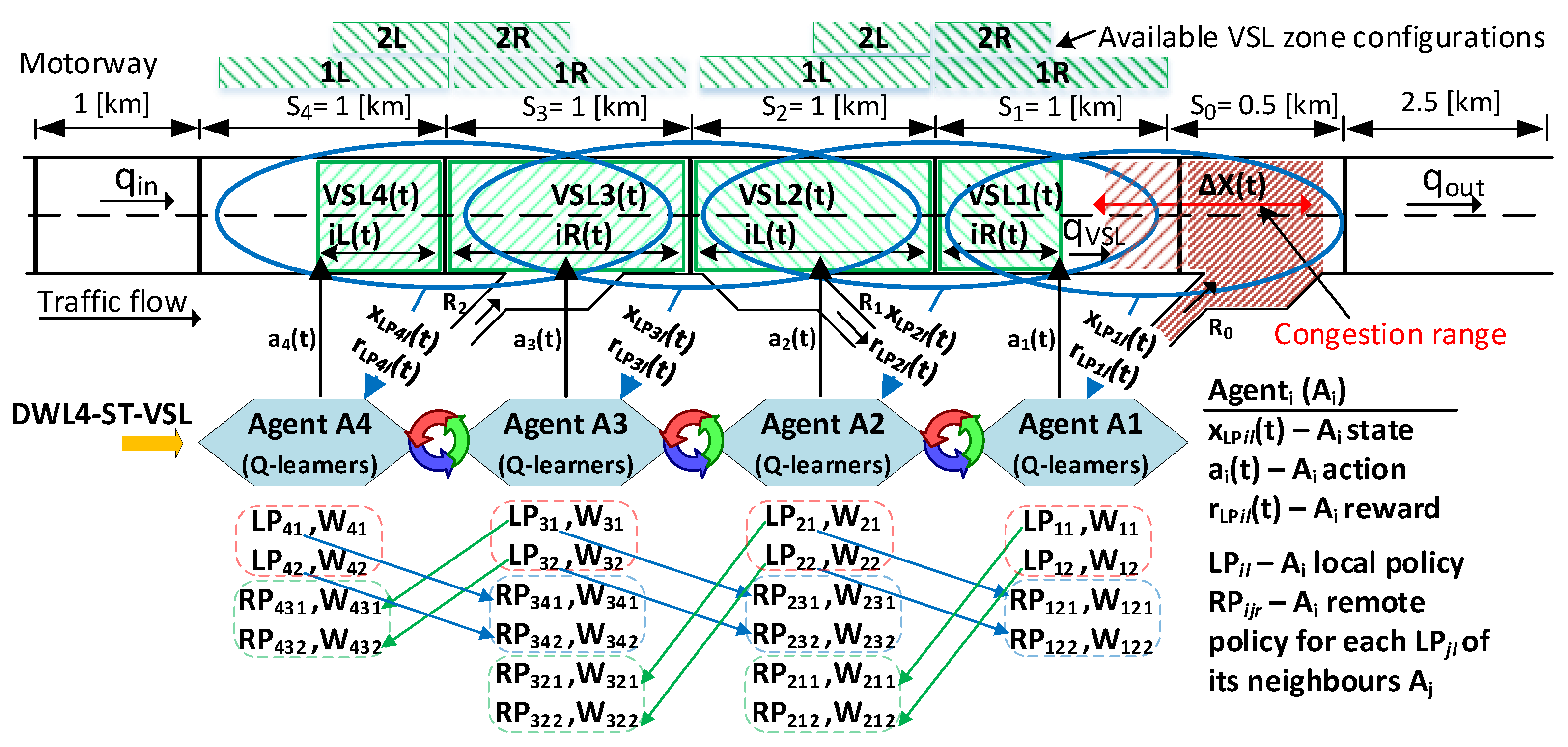
So far, DWL has been successfully applied to the problem of controlling urban intersections on a larger scale network with a larger number of agents [28]. DWL has also proven successful in the VSL control optimization problem [23] on a smaller motorway segment. Nevertheless, it has never been tested for its extended applicability to motorway traffic control with a higher number of deployed VSL agents. Thus, in our extended DWL4-ST-VSL framework, four neighbouring agents ($Ai,i=1,2,3,4$) control the speed limit and VSL zone configuration (length and position) on their own motorway section. Each agent in DWL4-ST-VSL perceives its local environment through agent states and rewards (see Figure 2). Thus, in the proposed multi-agent control optimization problem, the agent states $x_t$, actions $a_t$, and reward functions $r_{t+1}$ are modelled as follows.

4.1. State Description

As stated in [18], defining a compact Markovian state representation for motorways is difficult because many external factors influence traffic flow: e.g., weather conditions, motorway geometry (curvature, slope), etc., which are hard to model precisely. Augmenting the state by additional information, such as observing more sections (e.g., the density measured on the motorway section further upstream from the congestion location and the on-ramp queue length, primarily to provide a predictive component in terms of motorway demand [21]) or including information from the past in states, may improve the algorithm’s performance. Though this increases solution space, it can be overcome by the function approximation technique [18,40]. However, in DWL modelling, the observation of the agent’s neighborhood is available through remote policies. Nevertheless, the observability of the state must be assured. An example of a partially observable state is the usage of flow rate for states. From traffic flow theory, macroscopic variables describe traffic conditions (speed, density, flow). As a result of the nonlinearity of the fundamental diagram (flow-density relationship) [39], the same traffic flow rate can be observed for a density value below critical density with high speed (stable flow) and a density value above critical density with low speed (unstable flow). Thus, the traffic condition is uniquely determined by using the information of traffic density. Therefore, we use speed and density measurements to omit the agents’ confusion, thus uniquely determining traffic conditions. As a result, the negative effect of imperfect and incomplete perception of agents’ partially observable states in our MDP modeling is reduced.

The inclusion of the speed measurement of the neighboring segments into the state can enhance the learning process, particularly at the beginning of the learning process, when agents cause interference by randomly performing actions (exploration). Besides, low speed indicates traffic flow disruption provoked by congestion. Speeds are encoded in the variable $V_n$, which corresponds to the measured average vehicle speed ${\overline{v}}_{n,t}$ at time t in motorway section $S_n$ ($n=0,1,2,3,4$), as shown in Figure 2. Each speed measurement can fall into one of four intervals defined with boundary points ($50,76,101$ [km/h]).

Current traffic density ${\overline{\rho }}_{n,t}$ measured in the motorway section $S_n$, is stored in the variable $P_n$. Each measurement can fall into one of twelve intervals defined by the boundary points ($15,20,23,26,29,32,35,38,45,55,65$ [veh/km/lane]). Additionally, the state space contains information about the agent’s action from the previous control time step, thereby enabling modelling restrictions on the action space by making it state dependent, which is explained in more detail in the following subsection.

Therefore, $A1$’s local policy $L{P}_{11}$ at time t senses state $x=(a_{1,t-1},V_0,P_0,P_1)$, while $L{P}_{12}$$x=(a_{1,t-1},V_1,P_0,P_1)$. $A2$’s $L{P}_{21}$ senses state $x=(a_{2,t-1},V_1,P_1,P_2,)$, while $L{P}_{22}$$x=(a_{2,t-1},V_2,P_1,P_2)$. Similarly, $A3$’s $L{P}_{31}$ senses state $x=(a_{3,t-1},V_2,P_2,P_3,)$, while $L{P}_{32}$$x=(a_{3,t-1},V_3,P_2,P_3)$. Finally, $A4$’s $L{P}_{41}$ senses state $x=(a_{4,t-1},V_3,P_3,P_4,)$, while $L{P}_{42}$$x=(a_{4,t-1},V_4,P_3,P_4)$ (see Figure 2).

4.2. Action Space

Each element in the action sets (4) and (5) consists of two variables. The upper one represents the speed limit [km/h] in section $S_n$, while the lower one represents an active VSL zone (indexes for the left ($iL$)/right ($iR$) configuration; see Figure 2). Agent $A1$ controls the speed limit and the length of the VSL zone in section $S_1$, while $A2$ controls section $S_2$, and so on. In this way, the agent’s winning policy (either $L{P}_i$ or $R{P}_i$) will define the speed limit and the VSL zone configuration for a given motorway section.

$$\begin{array}{c}\hfill {\mathcal{A}}_{1,2,DWL}=\left\{\left\{\begin{array}{c}60\\ 1\end{array}\right\},\left\{\begin{array}{c}60\\ 2\end{array}\right\},\left\{\begin{array}{c}80\\ 1\end{array}\right\},\left\{\begin{array}{c}80\\ 2\end{array}\right\},\left\{\begin{array}{c}100\\ 1\end{array}\right\},\left\{\begin{array}{c}100\\ 2\end{array}\right\},\left\{\begin{array}{c}120\\ 1\end{array}\right\},\left\{\begin{array}{c}120\\ 2\end{array}\right\}\right\}\end{array}$$

(4)

$$\begin{array}{c}\hfill {\mathcal{A}}_{3,4,DWL}=\left\{\left\{\begin{array}{c}90\\ 1\end{array}\right\},\left\{\begin{array}{c}90\\ 2\end{array}\right\},\left\{\begin{array}{c}100\\ 1\end{array}\right\},\left\{\begin{array}{c}100\\ 2\end{array}\right\},\left\{\begin{array}{c}110\\ 1\end{array}\right\},\left\{\begin{array}{c}110\\ 2\end{array}\right\},\left\{\begin{array}{c}120\\ 1\end{array}\right\},\left\{\begin{array}{c}120\\ 2\end{array}\right\}\right\}\end{array}$$

(5)

Q-values in (DWL2 and DWL4)-ST-VSL are stored in a $Q_{\left|X\right|\times |A_{DWL}|}$ matrix, where X is a finite set containing the indices of the coded states of the Cartesian product of the input traffic variables ($\left|X\right| = 4608$ and $|A_{DWL}| = |A_{1,2,DWL}| = |A_{3,4,DWL}| = 8$). This seems to be a large solution space for learning optimal Q-values using (1). Nevertheless, the feasible solution space was reduced by constraining the action selection in the nomination process explained in the continuation. Thus, Q-matrix can be considered a sparse matrix, and there is no need to search the whole space.

The consecutive speed limit change within a section (n) must satisfy constraint $|a_{t-1,n}-a_{t,n}| \le 20$ in the case of agents $A1$ and $A2$, which use action set $A_{1,2,DWL}$. In the case of $A3$ and $A4$ ($A_{3,4,DWL}$), the constraint is $|a_{t-1,n}-a_{t,n}| \le 10$. This ensures a smooth and safe speed transition between the upstream free-flow and the congested downstream flow characterized by lower vehicle speeds due to the bottleneck. Thus, the final set of actions allowed for the agent $Ai$ at time t depends on the previously executed actions of the agent. This constraint also implies that the next possible action ($a^{\prime }$) in the update process of the W- and Q-values (see update rules (1) and (2)) must be bounded based on $a_t$. Thus, each time the Q-value is updated, a possible subset of the allowed actions is considered. E.g., if $a_{k,t-1}=A_{1,2,DWL}(7)$, then the available action subset at time t is $A{*}_{1,2,DWL}=\{A_{1,2,DWL}(5),A_{1,2,DWL}(6),A_{1,2,DWL}(7),A_{1,2,DWL}(8)\}$. Therefore, the previous action in the state space is used to uniquely distinguish between states’ transitions given the constrained subset of actions between control time steps. This constraint is implicitly modelled in the update rule (1). It addresses a unique row in Q-matrix ($Q(x,a)$) and the reachable entries in that row, corresponding to a given action index. Feasible entries in the particular row correspond to original indexes of elements from the original action set). Thus, only such entries in $Q(x,a)$ are reachable in updating Q- and W-values and in the action nomination process while using “argmax” in Q-learning. Otherwise, the oscillation in the values of elements in a particular state (row) will be present. Thus, Q-values will not converge to a stationary policy, and action nomination in a particular state will constantly switch no matter how long the learning period is. Eventually, a stable agent diminishes the nonstationarity effect in the learning problem of the other agents.

In this way, it is not necessary to model constraints directly in the rewards. It is still ensured that DWL4-ST-VSL operates according to the advised safety rules on maximum allowable speed changes.

It is important to note that the constraints on the spatial difference of speed limit values between two adjacent VSL zones on the motorway are not explicitly considered in this setup. It is assumed that agents communicate information about congestion intensity and locations via remote policies. Thus, the difference in spatial speed limits should be reasonable in terms of optimal traffic flow control. This is also aided by DWL’s ability to implement two sets of speed limits with different granularity simultaneously. Action set (4) is for agents $A1$ and $A2$, which are closer to the bottleneck. The finer action set (5) is for upstream agents $A3$ and $A4$. The finer actions aim to slightly adjust the speeds of the arriving vehicles before they enter the VSL application areas controlled by downstream agents. In this way, agents smooth out the incoming traffic towards the congestion point, thus avoiding the undesirable sudden deceleration of vehicles and effects such as shockwaves.

4.3. Reward Function

In [18], the minimization of the total time spent ($TTS$) of vehicles on the observed motorway segment over a given time interval was successfully used as an objective in RL-VSL control. Therefore, we also use the $TTS$ measure for reward. The variable $TT{S}_{n,t+1}$ measures $TTS$ between two control time steps t and $t+1$ on the motorway section n. In this way, an agent receives feedback about how good its action was. Each agent must learn to strike a balance between two conflicting policies. In the case of an inactive bottleneck, the penalty will be lower for a higher speed limit. Contrary, when congestion occurs, it is required to gradually reduce the speed limit in upstream sections to control the incoming traffic towards the congestion point so as to maintain the traffic volume near the operational capacity of the active bottleneck. Thus, each policy seeks to optimize its objective as follows.

4.3.1. Local Policy for Stable-Flow Control

The local policy $L{P}_{i1}$ of an agent $Ai$ aims to learn the speed limit to ensure a reduction of $TTS$ by promoting, when possible, higher traveling speeds in stable-flow conditions. To achieve this goal, the $L{P}_{i1}$ reward is:

$$r_{LPi1,t+1}=\left\{\begin{array}{c}0,\mathrm{if}min\left\{{\overline{v}}_{n,t+1}|n=i,i-1\right\} \ge 102\hfill \\ -TT{S}_{n,t+1},n=i\mathrm{otherwise}\hfill \end{array}\right.,$$

(6)

thereby favoring average vehicle speeds above 102 [km/h].

In a certain percentage, $L{P}_{i1}$ is activated in saturated flow during the transition from free-flow to congested flow and vice versa. Therefore, it prepares traffic for the second policy ($L{P}_{i2}$), which dominates in oversaturated (congested) conditions. After congestion has started to resolve by deploying $L{P}_{i2}$, and the congestion intensity reduces to a certain level, $L{P}_{i1}$ helps restore traffic to free flow (higher traveling speeds) as soon as possible by gradually increasing the speed limit. Thus, $L{P}_{i1}$ seeks to reduce traffic recovery time. Finally, the states perceived by $L{P}_{i1}$ satisfy the minimum requirements to determine whether the flow in the agent’s neighborhood is a stable flow or deviating from it. Thus, the agent can recognize when the higher speed limits for free flow can be implemented or not.

4.3.2. Local Policy for Unstable-Flow (Congested) Traffic Control

Local policy $L{P}_{i2}$ aims to reduce $TTS$ in the downstream motorway section in the case of an active bottleneck. Thus, an agent must learn and apply appropriate speed limits to restrict the inflow into the bottleneck until the discharge capacity is restored. If not, congestion will grow, and consequently, it will increase its penalty in proportion to:

$$r_{LPi2,t+1}=-\beta TT{S}_{n,t+1},n=i-1,$$

(7)

where coefficient $\beta$ controls the agent’s sensitivity to congestion. Instead of using only downstream congestion information, $L{P}_{i2}$ uses information about the upcoming traffic flow (current speed and density) from the section $S_n,n=i$. This can be considered a prediction of the forthcoming traffic flow (how fast and with what volume it will arrive) into the downstream congested section $S_n,n=i-1$. In this way, the description of traffic conditions (states) is extended to include more unique traffic characteristics for more efficient congestion control.

4.3.3. Remote Policies

Cooperation between agents is based on remote policies. Thus, an agent $Ai$ learns additional remote policies ($R{P}_{ij1},\dots ,R{P}_{ijr}$) that complement its neighbouring agent’s local policies. In order to know how $Ai$’s local actions $a_t$ affect the neighbours’ states, the agent updates the remote policies by the information it receives about its neighbours’ current states and the rewards that neighbour agents have received (Figure 2). Our experiments consider that agents’ communication is perfect (no loss of information and no breakdown of agents is assumed).

4.4. Winner Action

In DWL4-ST-VSL, an agent $Ai$’s experience (Q-values for local-state/action pairs and Q-values for remote-state/local-action pairs) for each policy are respectively stored in $Q_{ik}$ matrices. In the case of agents $A1$ and $A4$ ($k=1,\dots ,4$), while for $A2$ and $A3$ ($k=1,\dots ,6$). At the same time, for each of the states of each of its policies, an agent learns W-values of what happens in terms of the reward received if the action nominated by that policy is not performed [43]. This is expressed as a W-value ($W(x_{i,t})$) and stored in $W_{ik}$ matrices in each case. With the knowledge gained from these matrices, all policies (local and remote) propose new actions. The action $a_{k,t}$ that wins the competition between policies at this time step is the one with the highest W-value ($W_{max}$) (computed using (3)) [28]. After the state transition $x_t\mapsto x_{t+1}$, each agent’s local policy receives its unique reward ($r_{LPi1,t+1}$, $r_{LPi2,t+1}$) and state ($x_{LPi1,t+1}$, $x_{LPi2,t+1}$) depending on the consequences of the executed action $a_{k,t}$. The remote policies $R{P}_{ijr}$ obtain rewards and state information from their neighbour agent by querying the neighbour’s local policies states/rewards ($x_{LPj1,t+1}$, $r_{LPj1,t+1}$, $x_{LPj2,t+1}$, and $r_{LPj2,t+1}$). Then, all policies update their Q-values (for the winning action $a_{k,t}$), while only the policies that were not obeyed update their W-value. The above process is repeated for all agents.

5. Simulation Set-Up

To evaluate whether the dynamic assignment of VSL zones and cooperation between agents with DWL have an advantage over static VSL zones with non-cooperative agents, we compare DWL4-ST-VSL with our previous work on WL-VSL [24]. To verify the advantages of learning approaches over classical VSL control, we also compare DWL4-ST-VSL with SPSC [30]. It is important to note that the calibration procedure of the simulated motorway section is not included because a synthetic model with different traffic loads was used for this analysis. The objective of this study is to evaluate the impact of dynamically adjusting the VSL zone configurations and the different number of agents in DWL-ST-VSL on the optimization of traffic flow within an active bottleneck and the motorway as a whole.

5.1. Simulation Model

The simulation framework used consists of the microscopic simulator SUMO (version 1.8.0) and the Python programming environment. We referred to the software version because the simulation output in the new version may differ slightly from the simulation in the previous version, as the simulator source code is constantly being improved and updated.

The motorway model is based on the model used in [23]. It is divided into 5 main sections, $S_n,n=0,1,2,3,4$. To ensure all combinations of VSL zones used in these experiments (see Figure 2) and to measure spatio-temporal characteristics of the traffic flow, the entire simulation model is divided into smaller links (each 50 m long). The speed limit is simulated along with the computed configuration of the VSL zones for the chosen control time by directly assigning the allowed speeds to the corresponding links. The new speed limit and the configuration of the VSL zones are, thus, calculated by agents for each control time step $T_c=150$ [s]. In our previous work [23], this $T_c$ value was chosen from multiple tests. The used value is in the range of the foremost values found by the sensitivity analysis of control cycle lengths performed in [42]. The bottleneck is generated on the motorway section $S_0$. Each simulation lasts $1.5$ h, and all learning-based VSL approaches were trained in 14,000 simulations.

5.2. Traffic Scenarios

To evaluate the DWL4-ST-VSL control solution’s feasibility and behavior and determine whether agent cooperation and dynamic VSL zone assignment with DWL has advantages over VSL control approaches with static VSL zone configuration (WL-VSL and SPSC), we tested it under medium and high traffic loads. The input traffic data used were synthetic data, and the calibration process of the simulated model is not within the scope of this analysis. Therefore, the driver behavior and vehicle characteristics were modelled using the $Krauss$ car-following model with the default settings in SUMO [29].

5.2.1. Medium Traffic Load

In the downstream section $S_0$ (Figure 2), a bottleneck is induced by an increase in traffic demand at the on-ramp $R_0$. The generated bottleneck is the primary test for DWL4-ST-VSL with dynamic VSL zone allocation. In this traffic scenario, the demand at on-ramp $R_0$ changes over time (see Figure 3). For the highest demand at on-ramp $R_0$, 1315 [veh/h], slower vehicles entering the motorway interact with the mainstream traffic in the merge area. Consequently, this causes disturbances, which triggers the activation of the bottleneck, and congestion appears. Traffic flow at ramps $R_1$ and $R_2$ remain constant for both traffic scenarios, with the flow of 385 and 230 [veh/h], respectively. The mainstream flow entering the bottleneck area has a constant rate of 1385 [veh/h/lane]. The traffic flow consists of $94\%$ cars, $3\%$ buses and $3\%$ trucks.

5.2.2. High Traffic Load

The induced congestion is much more significant in this traffic scenario than in the medium scenario. In particular, an increase is generated by a $7.22\%$ higher traffic mainstream demand entering the bottleneck area relative to the medium traffic scenario. This is the test for DWL4-ST-VSL emphasizing the dynamic adjustment of VSL zones. Since the congestion tail propagates much more upstream through the motorway, it can be expected that different VSL zone configurations will be used compared to the medium traffic scenario.

5.3. Baselines of SPSC and WL-VSL

In the case of baselines, the best static VSL zone configuration $S_{2,(2L)}+S_{1,(1R)}$ (see Figure 2) and parameters were selected from several tests conducted for the medium traffic load.

In the case of SPSC [30], the gain ($Kv=4.5$) and activation threshold (traffic density of 23 [veh/km/lane]) were selected from several tests.

The same best static VSL configuration is also used for the WL-VSL case. In WL-VSL, two local policies were used. Local policy $L{P}_1$ aims to maintain a higher speed on controlled motorway sections, while $L{P}_2$ aims to reduce congestion in the presence of an active bottleneck. The observed state variables for $L{P}_1$ are densities within sections $S_1$ and $S_{2,(2L)}$, and for $L{P}_2$ densities within sections $S_0$ and $S_1$, the “bottleneck region”. Each element of the action set contains two variables (the section $S_1$ and $S_{2,(2L)}$ speed limits). In this way, the winning policy will set speed limits for both sections [24]. The two rewards associated with the mentioned policies were modelled as follows:

$$r_{LP1,t+1}=\left\{\begin{array}{c}0,\mathrm{if}min\left\{{\overline{v}}_{n,t+1}|n=0,1,2\right\} \ge 100\hfill \\ -0.4(2TT{S}_{2,(2L),t+1}+TT{S}_{1,(1R),t+1})\mathrm{otherwise}\hfill \end{array}\right.,$$

(8)

$$r_{LP2,t+1}=-TT{S}_{0,t+1}.$$

(9)

5.4. DWL-ST-VSL Parameters

For both (DWL2 and DWL4)-ST-VSL and WL-VSL we use the “learning Q (somewhat) before learning W” scheme [43], controlled by ${\alpha }_W{(1-{\alpha }_Q)}^{\omega }$ part in (2), where ${\alpha }_Q=\frac{1}{n(x,a)}$ and ${\alpha }_W=\frac{1}{n(x)}$ depend on the number of visits to $Q_i(x,a)$. Thus, the weight is larger when an agent is sure of what it is doing in a given state. This is indicated by a higher frequency of nominating a particular action based on the highest Q-value. The parameter $\omega =1.5$ controls how fast W converges and was selected from multiple tests. The author of WL [43], in his demonstrated example, used $\omega =3$. The parameter $\gamma =0.8$ was chosen from [24]. The exploration probability is decreased by the parameter $ϵ=exp\frac{-log(20)N}{6000}$, which decreases with the number of simulation runs N [23]. In the DWL-ST-VSL nomination process (3), the cooperation between agents is controlled by remote policies ($R{P}_i$) via a cooperation coefficient C. The cooperation levels we test are $C\in \left\{0,0.25,0.5,0.75,1\right\}$.

5.4.1. DWL2-ST-VSL Parameters

To keep the W-values of the local policies comparable to the W-values of the remote policies, we scale the reward function (7) by the factor $\beta =0.75$ in the case of agents $A2$ and for agent $A1$$\beta =1.25$. This is necessary because sections ($S_n,n=1,2$) are longer than $S_0$, which affects the final comparison in choosing the winning action since the W-values are bounded by $Q_{max}$ and $Q_{min}$. The bounds on the Q-values depend on the reward values $r_{min}$ and $r_{max}$ [43].

5.4.2. DWL4-ST-VSL Parameters

Similarly, to keep the W-values of local policies comparable to the W-values of remote policies in the case of DWL4-ST-VSL, we scale the reward function (7) by a factor $\beta =0.75$ for the case of agents ($Ai,i=2,3,4$) and for agent $A1$$\beta =1.25$.

6. Simulation Results

The VSL strategies are evaluated using the overall $TTS$ and measured on the entire simulated motorway segment (including ramps). Traffic parameters, average speed and density are measured in the bottleneck area (section $S_0$). The results presented in Figure 4, Figure 5, Figure 6 and Figure 7 are from the exploitation phase. We analyzed the specific response behavior of the allocation of dynamic VSL zones compared to the case of static zones. The space-time congestion analysis is used to analyze the spatiotemporal behaviour of dynamic VSL zone allocation and its impact on traffic flow control. To assess the benefits of cooperation between agents using DWL’s remote policies, we also evaluate the impact of the cooperation coefficient on agent performance. As a measure of the learning rate of proposed agent-based learning VSL approaches, the convergence curves of overall motorway $TTS$ during the training (learning) process are shown in Figure 8.

It is important to note that the purpose of this study is not to show the extent to which DWL4-ST-VSL can improve traffic, but to investigate how the dynamic (spatiotemporal) adaptation of VSL zone configurations and the increased number of learning agents affect the traffic control optimization problem. Thus, an improvement over baseline should be considered primarily as a comparative measure between two different VSL approaches, the commonly used static VSL zones and the new paradigm with dynamic VSL zone allocation, rather than as an absolute measure of performance.

6.1. Comparison of Dynamic VSL Zone Allocation and Static VSL Zones

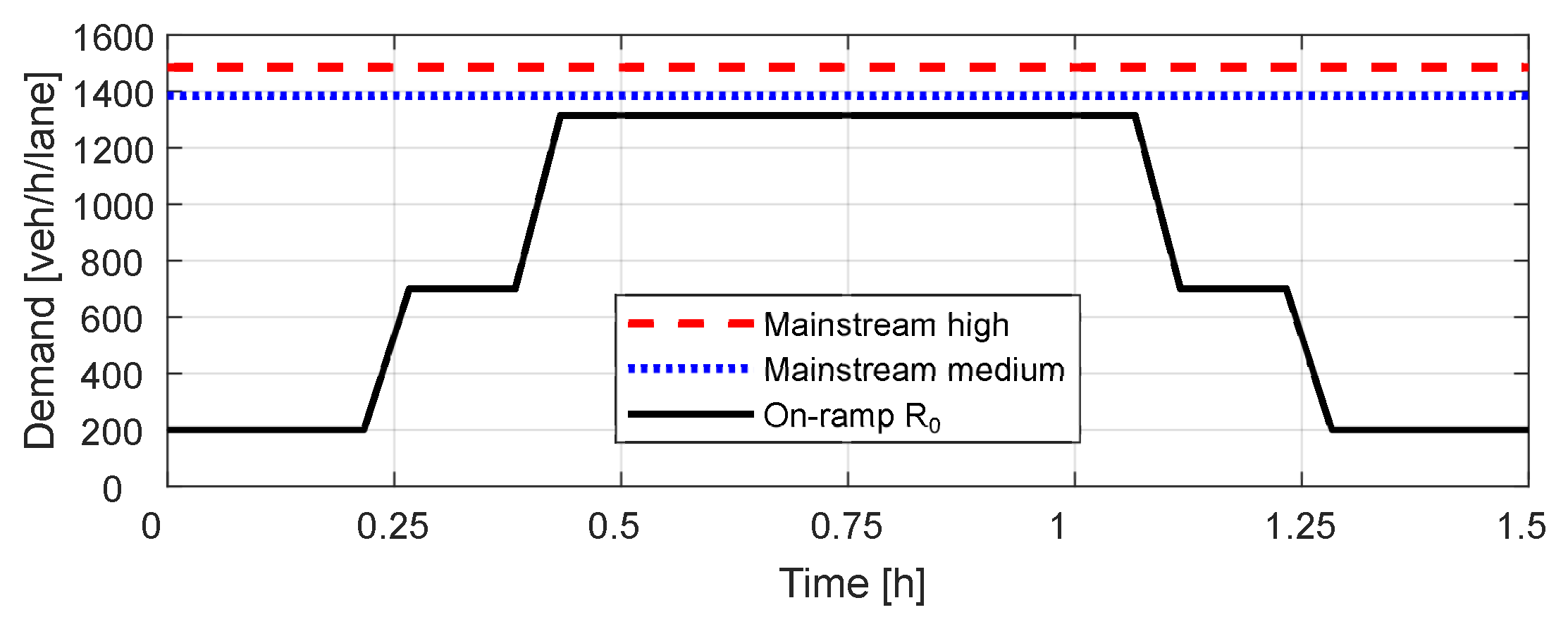
Note that the baselines use the best static VSL zone configuration found for a medium traffic load. Using a medium and a high load in our experimental setup, we simulate significant differences in the spatial displacement of the congestion tail. In this way, we illustrate the benefits and necessity of adaptive spatiotemporal VSL control. Different VSL zone configurations per traffic scenario are learned (without requiring manual setup) and dynamically assigned using DWL4-ST-VSL to better respond to spatially propagating traffic congestion. At the same time, the experiment highlighted the weaknesses of the static VSL zone configuration, which performs suboptimally under high traffic load. Therefore, the VSL zones in VSL with the static VSL zone configuration must be manually set up each time the traffic pattern changes, which is not practical.

6.1.1. Medium Traffic Load

The simulations performed show that the best combination for establishing static VSL zones is $S_{2,(2L)}+S_{1,(1R)}$. In this case, VSL is able to control congestion in the case of medium traffic load. In DWL2-ST-VSL, by additionally activating VSL zones within the $S_2$ section during the highest congestion peak (around $t=1$ [h]), the agent $A2$ helps its downstream neighbour $A1$, which contributes to an even more effective congestion resolution than the baselines (SPSC and WL-VSL) with static VSL zones. In DWL4-ST-VSL, the agents closest to the congestion ($A1$ and $A2$) are assisted by upstream agents ($A3$ and $A4$) that activate additional VSL zones within $S_3$ and $S_4$ just before the highest congestion peak ($t=1$ [h]) (for a shorter period than DWL2-ST-VSL). In this way, agents $A3$ and $A4$ help their downstream neighbours. Similar results to those found for DWL2-ST-VSL were observed.

6.1.2. High Traffic Load

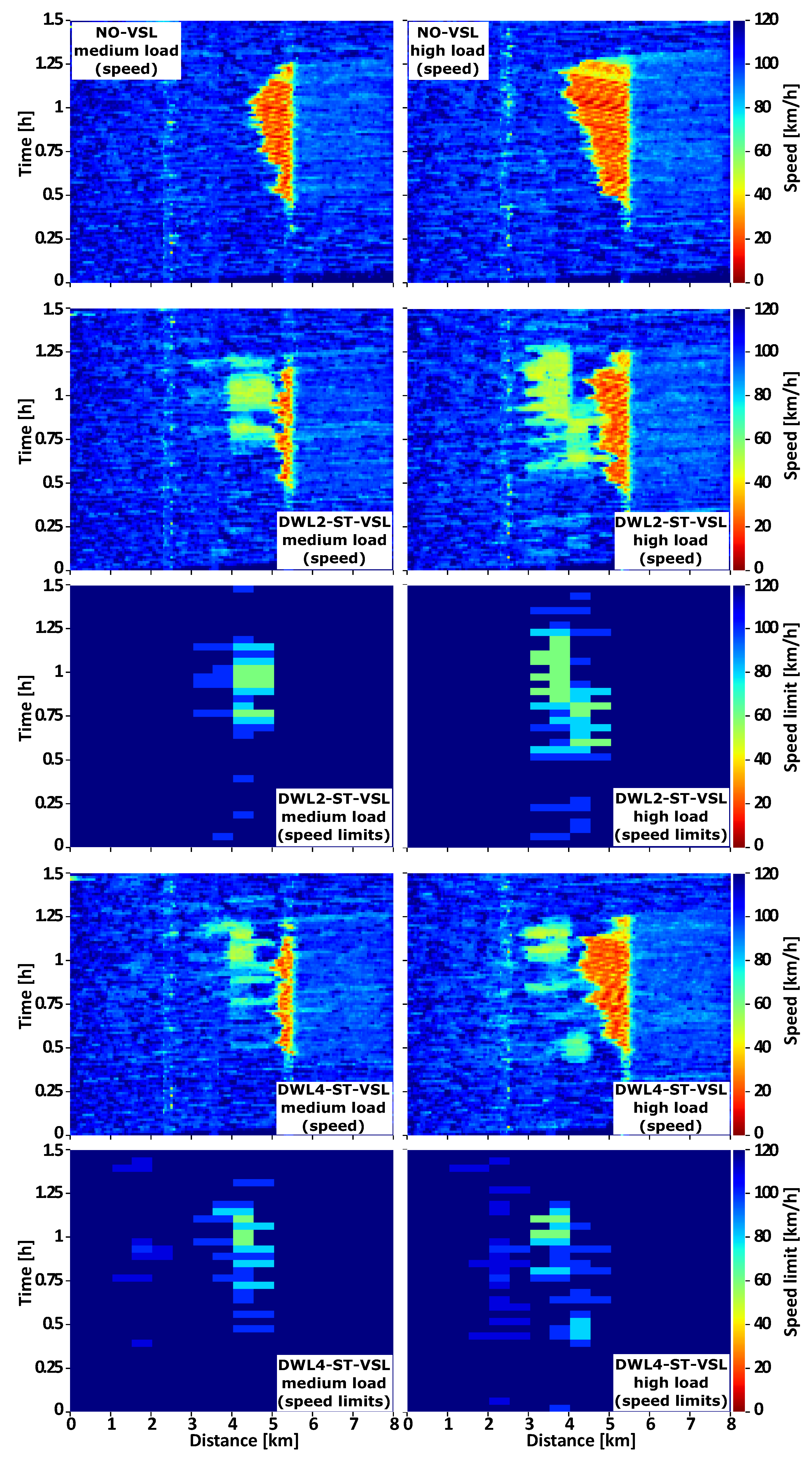
The performed simulations indicate that the static VSL zones perform suboptimally in a high traffic scenario. By applying different VSL zone configurations during the simulation within $S_n,n=1,2$ by DWL2-ST-VSL, and within sections $S_n,n=1,2,3,4$ in the case of DWL4-ST-VSL, they contribute more notably to congestion clearing than baselines, which results from the gradual adjustment of the VSL application area. In the DWL2-ST-VSL case, agents started with stronger activation of the speed limits and VSL zones in section $S_1$ at the beginning of the congestion. Over time, the congestion starts to propagate upstream through the motorway. The agents begin to use the VSL zones principally in sections $S_1$ and $S_2$, while finally, for the highest congestion peak, the VSL zones are primarily activated in section $S_2$.

In the case of DWL4-ST-VSL, VSL zones are activated mainly in all VSL sections at the onset of congestion (somewhat more sparsely for agent $A3$, while agent $A4$ was almost not activated at all). Agents $A1$ and $A2$ preferred a shorter VSL zone configuration, while $A3$ preferred a longer one. The application of shorter VSL zones in the downstream sections $S_1$ and $S_2$ could be due to the additional support provided by the upstream agents, particularly the speed limits applied by agent $A3$, which reduced the need for longer VSL zones and sudden decreases of the speed limit. As congestion increases, it can be seen in Figure 5 that the area of inactive VSL zones increases between upstream and downstream sections, primarily due to the use of shorter VSL zones by agent $A3$ and sparsely activated VSL zones by $A2$. After $t=0.75$ [h], agent $A2$ starts applying speed limits again in response to the sudden increase of the queue ahead of the bottleneck (faster propagation of the congestion upstream through the motorway). As congestion intensity approaches its peak, agent $A2$ promotes a longer VSL zone, including lower speed limits. Agent $A1$ is mostly inactive during this time period, thus forming an additional valuable transition zone [26] between the active VSL application area and the congestion tail. A somewhat unexpected behavior during the highest congestion peak is observed for agent $A4$, which did not apply speed limits below 120 [km/h] while $A3$ was not active for 3 control steps (Figure 5). In the next section, we will make some arguments that we believe can help explain this unexpected agent behavior.

Nevertheless, both DWL2-ST-VSL and DWL4-ST-VSL adjusted the VSL zones to the spatially moving tail of the resulting congestion. This control strategy is more pronounced in the case of the high congestion scenario, in which agents attempt to create an additional artificial moving bottleneck to reduce the outflow from it and, thus, relieve the congested area. From Figure 5, it can be seen that the agents aim to create such a VSL configuration that ensures the additional space (without speed limit) between the VSL zones and the congested tail. This can be viewed as an acceleration zone after the VSL zone, allowing vehicles to accelerate to the critical speed (at which capacity is reached) before entering the congested tail, as indicated in [25]. This feature of DWL-ST-VSL is very useful compared to the static VSL zone (fixed configuration) and confirms the findings that the higher the speed limit, the farther the VSL application zone should be from the bottleneck, which has been recently proven analytically in [26].

6.2. Space-Time Congestion Analysis

Space-time diagrams are interesting for visualizing how traffic conditions evolve along the observed motorway segment. The on-ramp $R_0$ in $S_0$ is located at $x=5.3$ [km]. DWL2-ST-VSL ranges from $x=3$ to $x=5$ [km], while DWL4-ST-VSL ranges from $x=1$ to $x=5$ [km]. The best configuration of the static VSL zones (WL-VSL, SPSC) ranges from $x=3.5$ to $x=5$ [km]. The initial transition area [26] after the VSL zone starts at $x=5$ [km] to the on-ramp $R_0$ and can be changed if the configuration of the VSL zones changes during agents’ operations in DWL-ST-VSL (in particular $A1$ and $A2$).

6.2.1. Medium Traffic Load

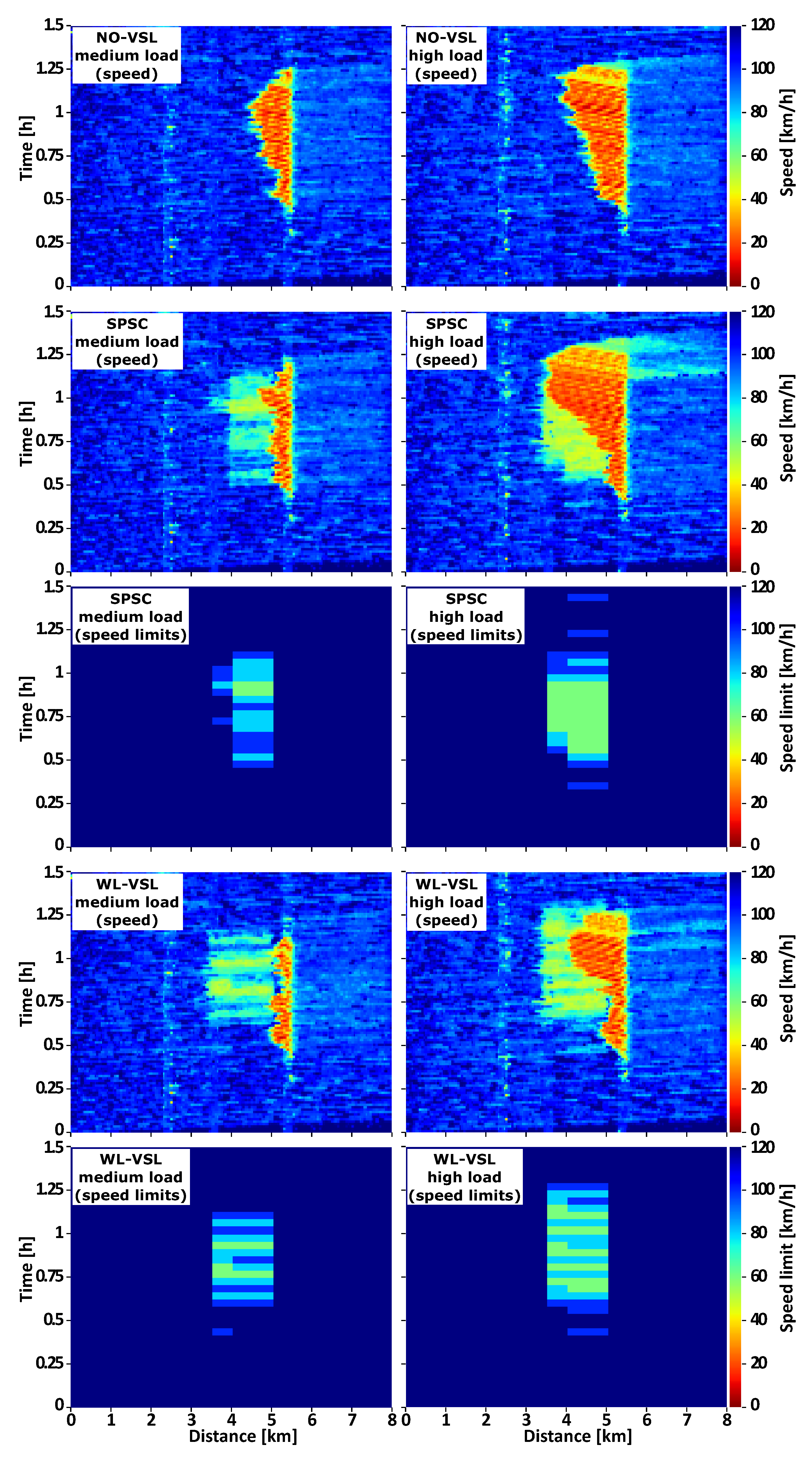
In Figure 4 and Figure 5, the mixed shades of red and orange correspond to congestion where vehicles are traveling at low speeds. The patterns of red stripes represent the propagation of the shock wave upstream through the motorway. Congestion begins at about $t=0.4$ [h] in the bottleneck area and propagates upstream. After the demand on the on-ramp $R_0$ decreases, the congestion decreases and finally dissipates at $t=1.25$ [h].

In both DWL-ST-VSL control strategies, the congestion (red) area is much smaller than in the baseline cases. The mixed shades of yellow-green-light blue in front of the congestion area correspond to the speed of vehicles obeying the speed limits (60–100 [km/h]) within active VSL zones. Such an artificially generated moving bottleneck (adaptive VSL area) with a significantly higher average travelling speed than the one measured in the congestion area still reduces inflow into the congestion area, which helps to resolve congestion more efficiently than baselines. In response to spatially varying congestion, both DWL-ST-VSL produce more stable downstream flow than the best baselines with static VSL zones. In the medium load scenario, congestion propagates upstream from the bottleneck to location $x=4.4$ [km]. In the case of DWL2-ST-VSL and DWL4-ST-VSL, the propagation is reduced to $x=5$ [km], which is an improvement of $66.7\%$ compared to NO-VSL. Finally, the average density in the congested area (bottleneck $S_0$ and directly affected upstream section $S_1$) is reduced from $26.0$ in NO-VSL to $20.0$ [veh/km/lane] in the case of DWL2-ST-VSL, an improvement of $23.1\%$. The improvement for simulated DWL4-ST-VSL is $20.8\%$.

6.2.2. High Traffic Load

Again, both DWL-ST-VSL versions win the competition. For DWL2-ST-VSL and DWL4-ST-VSL, the congestion area is smaller than for baselines. During the simulated scenario, different combinations of VSL zones were applied to respond to the changing congestion intensities and moving congestion tail. In this way, DWL2-ST-VSL and DWL4-ST-VSL are able to reduce the congestion area much more effectively than the baselines with static VSL zones. In the case of NO-VSL for the high-load scenario, the congestion spreads upstream from the bottleneck to the location $x=3.8$ [km]. When DWL2-ST-VSL is applied, the propagation is reduced to near $x=4.4$ [km], an improvement of $40\%$. Using the extended version with four agents (DWL4-ST-VSL), propagation is reduced to about $x=4.2$ [km], an improvement of $26.7\%$. Finally, the average traffic density in the congested area ($S_0$ and $S_1$) is reduced from the original $34.1$ to $28.7$ [veh/km/lane] by using DWL2-ST-VSL, an improvement of $15.8\%$. In the case of DWL4-ST-VSL, the improvement achieved is $14.7\%$. Just for comparison, in the case of WL-VSL with static zones, the congestion propagates near $x=4$ [km], resulting in negligible improvement. A similar behavior is observed in the case of SPSC, eventually degrading the system performance.

6.3. Level of Cooperation Analysis

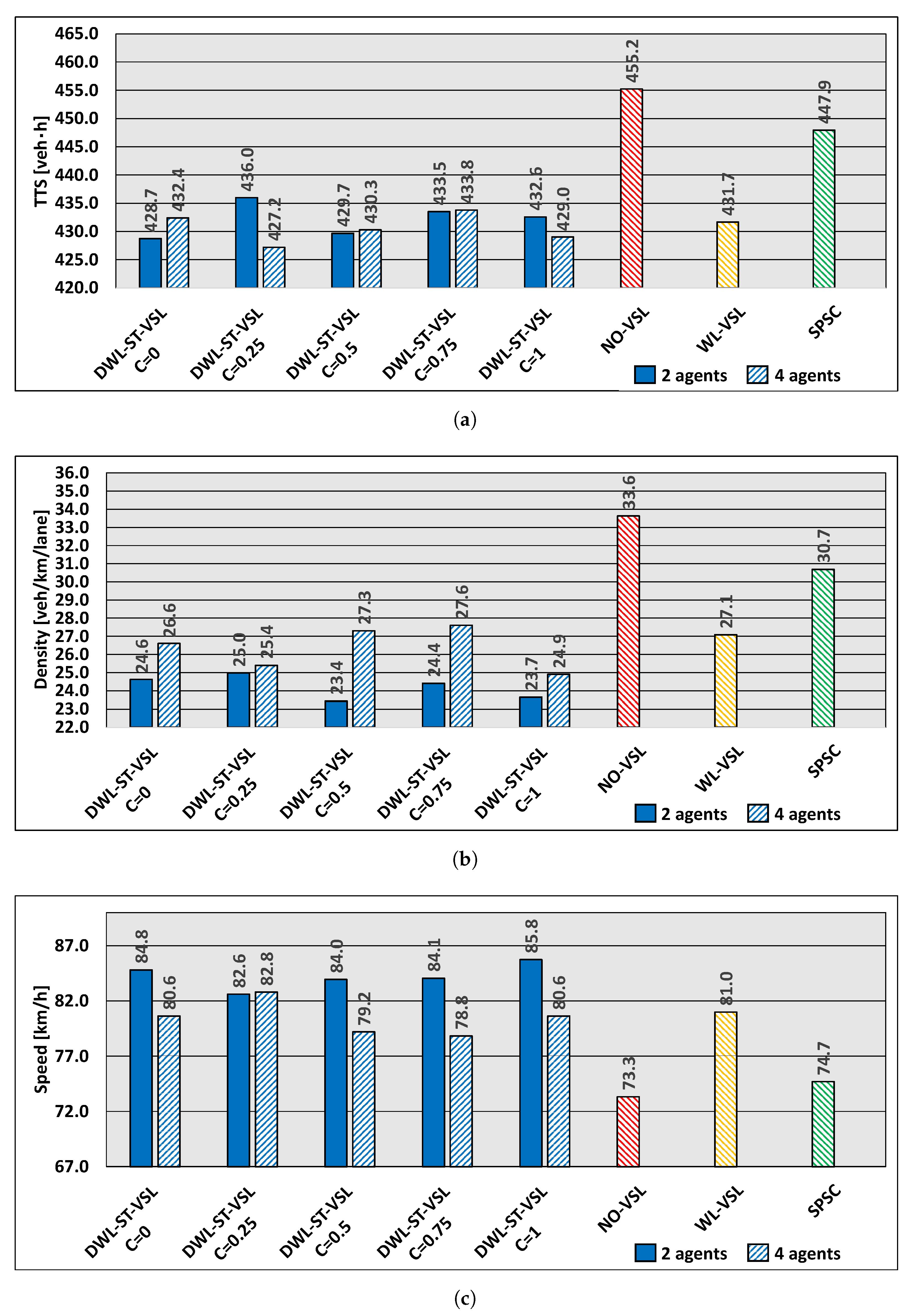
To evaluate the benefits of cooperation between agents using the DWL’s concept of remote policies, we also assess the effects of the cooperation coefficient on agent performance. The effects of different levels of agent collaboration on system performance are presented in Figure 6 and Figure 7. The analysis was performed for medium and high traffic loads (Figure 3).

6.3.1. Medium Traffic Load

It can be seen that all DWL-based approaches outperform the baselines used in our experiment. The lowest $TTS$ value is obtained with DWL4-ST-VSL and is $427.2$ [veh·h] for $C=0.25$. Compared to the NO-VSL case, ($TTS=455.2$ [veh·h]), a reduction of $6.2\%$ (Figure 6a). The best density is $23.4$ [veh/km/lane] for $C=0.5$ in the case of DWL2-ST-VSL, while it is $33.6$ for the case of NO-VSL, an improvement of $30.4\%$ (Figure 6b). In particular, the average vehicle speed for $C=1$ in the case of DWL2-ST-VSL is $85.8$ [km/h], while the speed in the case of NO-VSL is $73.3$ [km/h], an improvement of $17.1\%$ (Figure 6c).

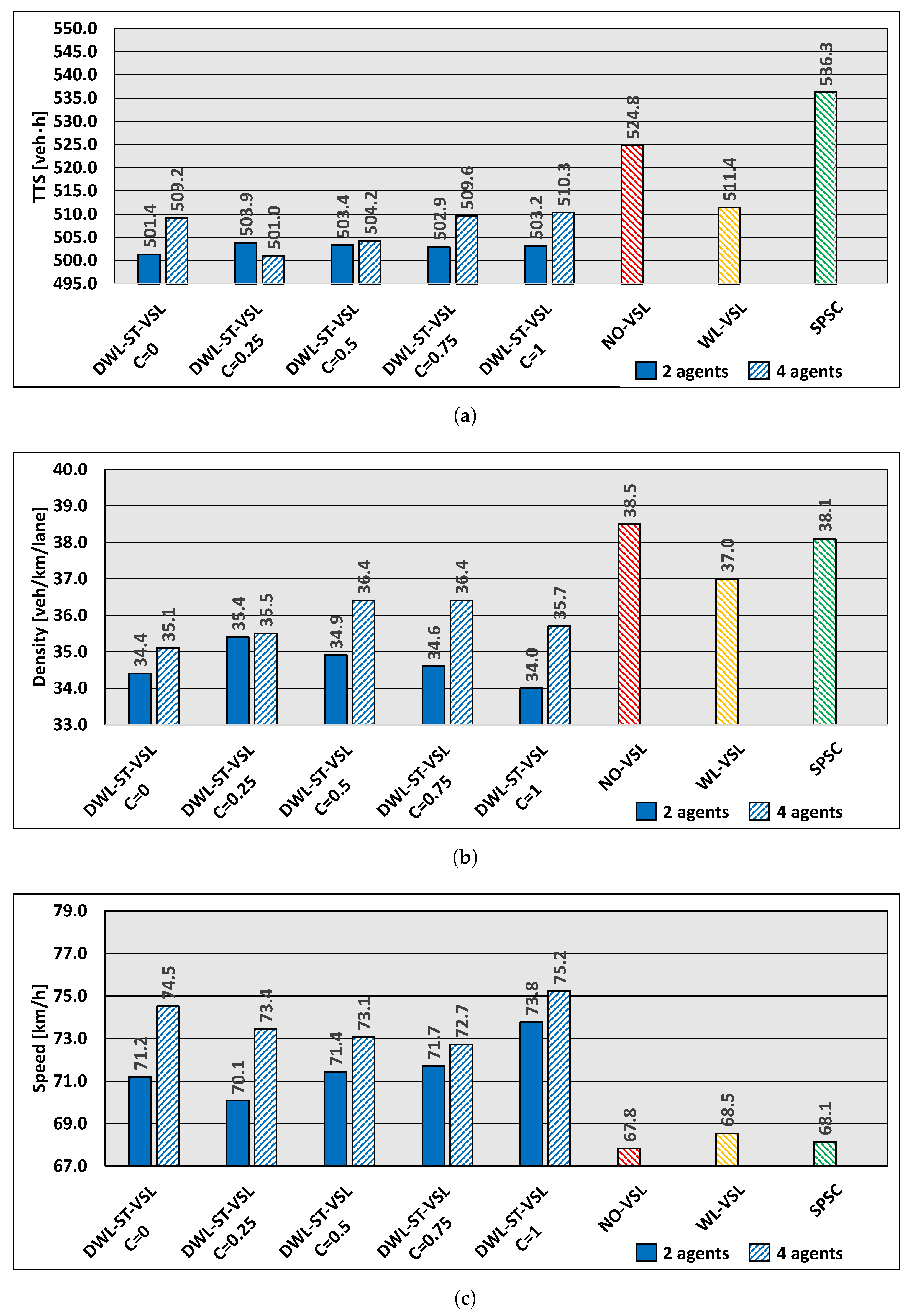
6.3.2. High Traffic Load

Similar results were obtained in the high traffic load experiment, where both DWL-ST-VSL configurations outperform the baseline controllers. The lowest $TTS$ value in the cooperative agent case in DWL4-ST-VSL is $501.0$ [veh·h] for $C=0.25$. Compared to the NO-VSL case, ($TTS=524.8$ [veh·h]); this is an improvement of $4.5\%$ (Figure 7a). The density is $34.0$ [veh/km/lane] for DWL2-ST-VSL ($C=1$), while in the case of NO-VSL it is $38.5$, a reduction of $11.7\%$. The density is reduced by $7.8\%$ by using DWL4-ST-VSL (Figure 7b). In particular, in the case of DWL2-ST-VSL, the average vehicle speed for $C=1$ is $73.8$ [km/h], while in the case of NO-VSL the speed is $67.8$ [km/h], an improvement of $8.8\%$ (Figure 7c). In the case of DWL4-ST-VSL, the average speed is $10.9\%$ higher (for $C=1$).

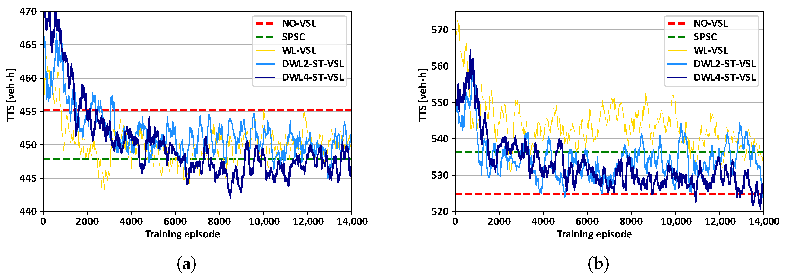
6.4. Convergence of $TTS$ during the Training Process

A comparison of the convergence of $TTS$ measured per training episode (episode $\equiv$ one simulation) during the learning process is shown in Figure 8. The graphs are created using the moving average over 10 episodes, while $TTS$ was measured in the entire motorway network (including all on- and off-ramps). At the beginning of the learning process, all agent-based VSL approaches performed inferiorly compared to NO-VSL, since agents explore the environment by executing random actions with high probability. As simulations progress, the number of random actions taken reduces, and the exploitation of learned experiences increases. Consequently, $TTS$ decreases, indicating progress in learning. Due to the different complexities of proposed RL-based multi-agent VSL controllers, the different decrease rate of $TTS$ can be observed throughout the learning process. From Figure 8a, it can be seen that all approaches have stable decreasing learning curves; generally, DWL4-ST-VSL leads in $TTS$ reduction over other strategies in the medium traffic scenario.

For the high traffic scenario (Figure 8b), the static VSL zones used in WL-VSL are prone to performing poorly compared to the dynamic VSL zones. Cases with dynamic VSL zone allocation via DWL2-ST-VSL and DWL4-ST-VSL need a higher number of training episodes to approach lower $TTS$ values. As the learning process approaches 14,000 episodes, $TTS$ in the case of DWL2-ST-VSL and DWL4-ST-VSL converges moderately towards and below the $TTS$ value obtained in NO-VSL. Eventually, compared with the starting values, the overall $TTS$ is gradually improved for all agent-based VSL strategies, favouring the learning rate of DWL4-ST-VSL in both traffic scenarios.

In the case of the high traffic scenario (Figure 8b), it can be seen that DWL4-ST-VSL needs a slightly longer time, i.e., higher number of training episodes (around 11,000) to reduce $TTS$ below the value obtained by NO-VSL. Nevertheless, when converted in real-time, it takes roughly 90 [h] of training in a simulator (on an Intel(R) Core(TM) i7-10750H CPU processor). In case our simulated experiment represents actual recurrent traffic congestion observed online, DWL4-ST-VSL can be trained offline (on simulations) and deployed in a real application in a short period. Thus, DWL4-ST-VSL can be retrained offline to deal with traffic changes in the operating environment to ensure good performance in the newly observed traffic scenarios (similar to the continuous learning scheme for Q-Learning based VSL suggested in [17]).

The longer time needed for reaching the favorable level may be directly linked to the larger number of agents. They eventually need more training episodes to become aware of the interference they cause by their actions on their immediate neighbours and the controlled motorway system as a whole.

In the second half of the learning process, there are more pronounced oscillations in $TTS$. The possible contribution to this might be delaying W’s convergence until Q is well known (see Section 5.4). Thus, W-values are more altered as Q-values are more learned. Consequently, this influences the policies’ nomination (3) in the DWL process and eventually influences the cooperation strategies between agents. As a result, it might cause a change in a learned set of optimal policies, thus resulting in the different system responses during the second half of the learning process. The new policy can induce new rarely seen system states that have not been encountered before, thus affecting agents’ poor decisions. Nevertheless, the function approximation techniques can address this problem by ensuring better generalization (reasonable outputs) for rarely seen states, thus stabilizing the training (learning) process.

7. Discussion

The outermost agents ($A3$ and $A4$) do not perceive congestion directly and, therefore, tend to exploit local stable traffic conditions by promoting higher speed limits and, in particular, favoring their local policy $L{P}_{i1}$. As a result, for small values of the cooperation coefficient C, they do not fully contribute to helping downstream agents to eliminate the congestion. This raises the question of whether C should be scaled differently depending on the spatial location of the agents rather than using uniformly distributed equal values for all agents. It might make sense to increase the coefficients of C the farther agents are from the location of the bottleneck so that they are more sensitive to the preferences of downstream agents and, therefore, give more priority to remote policies in the case of active congestion. The question then arises: to what extent?

The converse is also true, since the actions of the downstream agents affect the state variables (in particular, the measured average vehicle speed) of the upstream agents. The upstream agents always observe the average speed in their immediate downstream area (in the case of local policy $L{P}_{i1}$) and, possibly, the actions performed by the downstream agents (lower speed limits) reduce the chance of winning the $L{P}_{i1}$; therefore, a penalty by the measured $TTS$ is more likely, even if the local environment is in free-flow conditions. This dependence is implicitly communicated to the downstream neighbouring agent $Aj$ in the form of a higher W-value for remote policy $R{P}_{ji1}$, which complements the local policy $L{P}_{i1}$ of the upstream agents $Ai$.

The above observation shows the possible trade-off in choosing optimal values for C. A feasible solution to make $Cs$ adaptive is to use a scaling scheme used in (2) “learning Q (somewhat) before learning W” [43]. In this scheme, the updates of W-values are weighted differently. The weighting is higher when an agent is sure of what it is doing in a given state. Given that the underlying DWL process (WL algorithm) is considered as a “fair” resolution of competition, this leads to the question: can the W-values of local policies, together with the probability of nominating a particular action in a given state, be communicated between neighbors and used as input for computing C? This may trigger further research on adaptive cooperation coefficient C.

Furthermore, the overlapping states of the environment, including the downstream neighbourhood (see Figure 2), has positive and negative effects on the agent’s learning behavior. The negative effect arises from the nonstationarity caused by the neighbours’ actions, resulting in a moving learning target (particularly during the exploration phase in the training phase) since agents are learning simultaneously. Thus, each time, Ai’s policy changes might cause other agents’ policies to change, too [50]. The positive effect is the agent’s ability to detect and respond to the early impulse of congestion in downstream traffic. All learning-based approaches were trained with the same number of simulations. However, due to nonstationarity, DWL4-ST-VSL may require more simulations to converge to better control policies for a given traffic scenario due to a higher number of agents. Therefore, DWL4-ST-VSL (and the final results) may be in a slightly unfavorable position compared to DWL2-ST-VSL.

In our experiments, we assumed that all measurements (traffic data) in our experiments are perfect. In reality, sensors are not ideal, and raw data needs to be analyzed and filtered before being used for traffic state estimation. Thus, accurate traffic states are important for real-time traffic control. Raw traffic flow data collected from sensors might be contaminated by different noises caused by the imperfection or damage of sensors. In [51], the authors introduced data denoising schemes to suppress the potential data outliers from raw traffic data for accurate traffic state estimation and prediction. This presents an open question for further research.

Additionally, the efficiency of DWL-ST-VSL is highly dependent on the learning process performed in traffic simulations. Since simulations themselves depend on the given initial parameters, not all possible relevant traffic conditions can be covered. A possible direction to improve the training process of DWL-ST-VSL by ensuring that all relevant traffic scenarios are covered is to use the idea of structured simulations. Originally proposed in [52], structured simulations are intended for testing the behavior of complex adaptive systems in general by changing the inputs into the simulations in a structured way. Such a framework might augment existing traffic scenarios (real or synthetic) with unprecedented scenarios that evoke or replicate important aspects of real traffic, such as rarely seen traffic states in which VSL agents performed poorly. Thus, a structured simulations approach can enrich the training data set and consequently minimize unexpected behavior of the RL-based VSL controller in practice.

Even under a medium load scenario, the resulting congestion on the motorway can be classified as a serious traffic problem. However, it has been shown that DWL2-ST-VSL and DWL4-ST-VSL can effectively resolve the congestion in this scenario due to their added ability to dynamically adjust the VSL zone configurations. Since the DWL agents could not fully handle the congestion in the high load scenario (even when using four agents), it might be useful to extend the DWL4-ST-VSL control, e.g., by integrating it with the merge control using the DWL multi-agent framework.

Experimental results confirmed the usefulness of using dynamic VSL zone allocation (the capability to adapt the VSL application area) while optimizing speed limits in traffic conditions with varying congestion. Similarly, in [42], a VSL strategy able to adjust each control cycle’s length (duration) online, given the changes in traffic conditions, was shown to be superior compared to a fixed cycle length. Thus, integrating dynamic VSL zone allocation and dynamic control cycles can make VSL more adaptive, making VSL’s performance more robust when operating in a nonstationary environment like a motorway. To accomplish the full benefits of adaptivity, the principal time constants of the system should be long enough for the system to ignore false disturbances and yet short enough to respond to indicative changes in the environment (the “stability-plasticity dilemma”) [53]. Therefore, further research in this direction is desirable in DWL-ST-VSL.

The VSL control approaches with static VSL zone configuration performed poorer in high traffic scenarios than those with dynamic VSL zone allocation. Thus, results strongly indicate the need for the adaptive speed limit system in speed limit, length and position of VSL zones to efficiently cope with the unpredictable spatio-temporal varying congestion, which is more likely to be the case in a real traffic scenario.

8. Conclusions

This paper presented DWL-ST-VSL, a multi-agent RL-based VSL control approach for the dynamic adjustment of VSL zones and speed limits. In addition, an extended version, DWL4-ST-VSL, was analyzed for an urban motorway simulation scenario where four agents learn to jointly control four segments ahead of a congested area using the DWL algorithm on a longer motorway segment. The simulations show that DWL4-ST-VSL and the two-agent based DWL2-ST-VSL consistently perform better than our baseline solutions, WL-VSL and SPSC. The results do not differ significantly between DWL2-ST-VSL and DWL4-ST-VSL in terms of bottleneck parameters. In terms of system travel time, DWL4-ST-VSL gives better results. VSL control is improved by simultaneously adjusting speed limit values and VSL zone configuration in response to spatiotemporal changes in congestion intensity and the congestion’s moving tail. In addition, performance is improved by DWL’s ability to implement multiple different policies simultaneously and to use two sets of actions with different speed limit granularity, as well as to enable collaboration between agents implementing remote policies.

However, the efficiency of DWL-ST-VSL is highly dependent on the training process performed in simulations. To train DWL-ST-VSL in a structured way and ensure that all relevant traffic simulation scenarios are covered, we will use the structured simulations mentioned in the discussion. Using structured simulations and the nonlinear function approximation technique for better generalization together with sensitivity analysis of hyperparameters in DWL may reduce the poor performance of DWL in a nonstationary motorway environment, thus fostering DWL-ST-VSL to be closer to testing in reality. Eventually, this will enable the systematic evaluation of adaptive DWL-ST-VSL control.

Additionally, the results suggest that there may be multiple local optima for different coefficients of cooperation, which requires further analysis. How resilient the learning system would be to the loss of information exchange if one or more agents failed, which is often the case in a real scenario where sensors and equipment are imperfect and may break down, highlights the open research directions. We will consider implementing additional degrees of freedom to allow each agent of DWL-ST-VSL to adjust the length and position of the VSL zone in both directions, considering the constraints on the spatial difference of the speed limit between two adjacent VSL zones. Finally, we will consider integrating DWL-ST-VSL with dynamic control cycles and merge control, as this could further advance the VSL system toward instantaneous vehicle speed control in the presence of emerging vehicle-to-infrastructure technologies and traffic control on motorways in general.