
Rock Segmentation in the Navigation Vision of the Planetary Rovers


Abstract
:
1. Introduction
- (i)
- This research proposed a synthetic algorithm and transfer learning-based framework, which provides a labor-saving solution for the rock segmentation in the navigation vision of the planetary rovers.
- (ii)
- This research proposed a synthetic algorithm and a synthetic dataset, which aid the research into the rock segmentation in the navigation vision of the planetary rovers.
- (iii)
- This research came up with an end-to-end (E2E) network (NI-U-Net++) for the pixel-level rock segmentation, which achieved state-of-the-art in the synthetic dataset.
2. Methods
- (1)
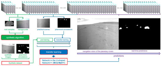
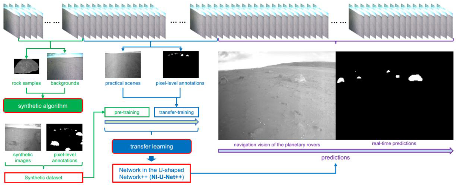
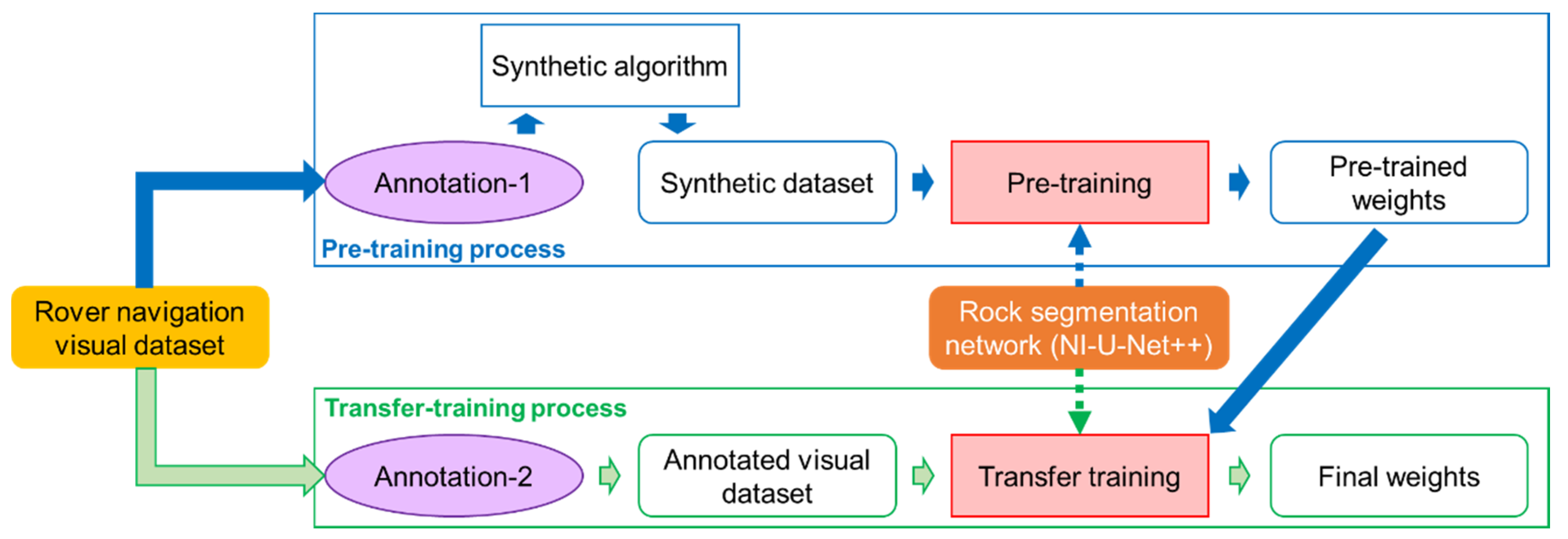
- The framework can be divided into two processes. Figure 1 identifies the pre-training process and the transfer-training process with the blue and green frames, respectively. Rock segmentation in an unannotated scenario is significantly difficult, and the transfer learning strategy divides the learning process into two steps. Although the synthetic dataset can generate large amount of pixel-level annotated data, they inevitably have a significant difference from the real-life data. The real-life data represent the practical mission, while its annotation corresponds to an expensive cost. Therefore, a cooperated solution between the synthetic data and real-life images becomes very promising. The pre-training process aims to achieve prior knowledge from a similar scene, and then, the transfer-training process fine-tunes the pre-trained weight to fit the real-life images.
- (2)
- In the pre-training process:
- (a)
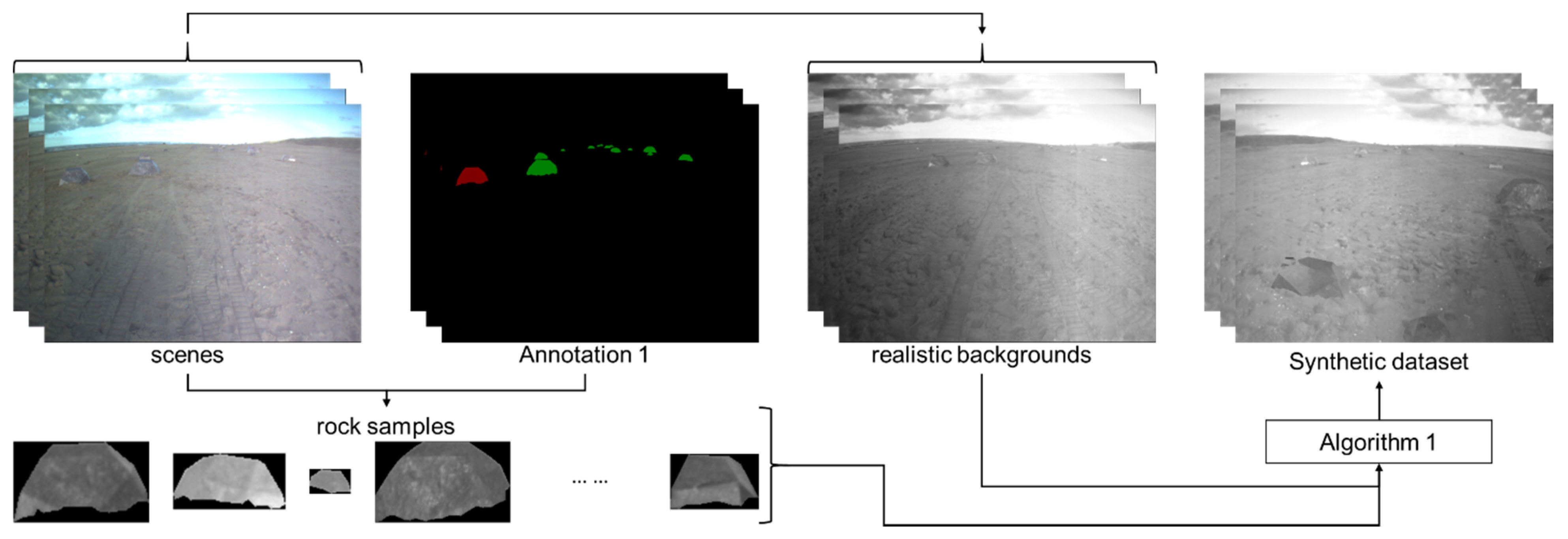
- The purple ellipse with “Annotation-1” refers to the first manual annotation, which aims to acquire the backgrounds and rock samples for the synthetic algorithm.
- (b)
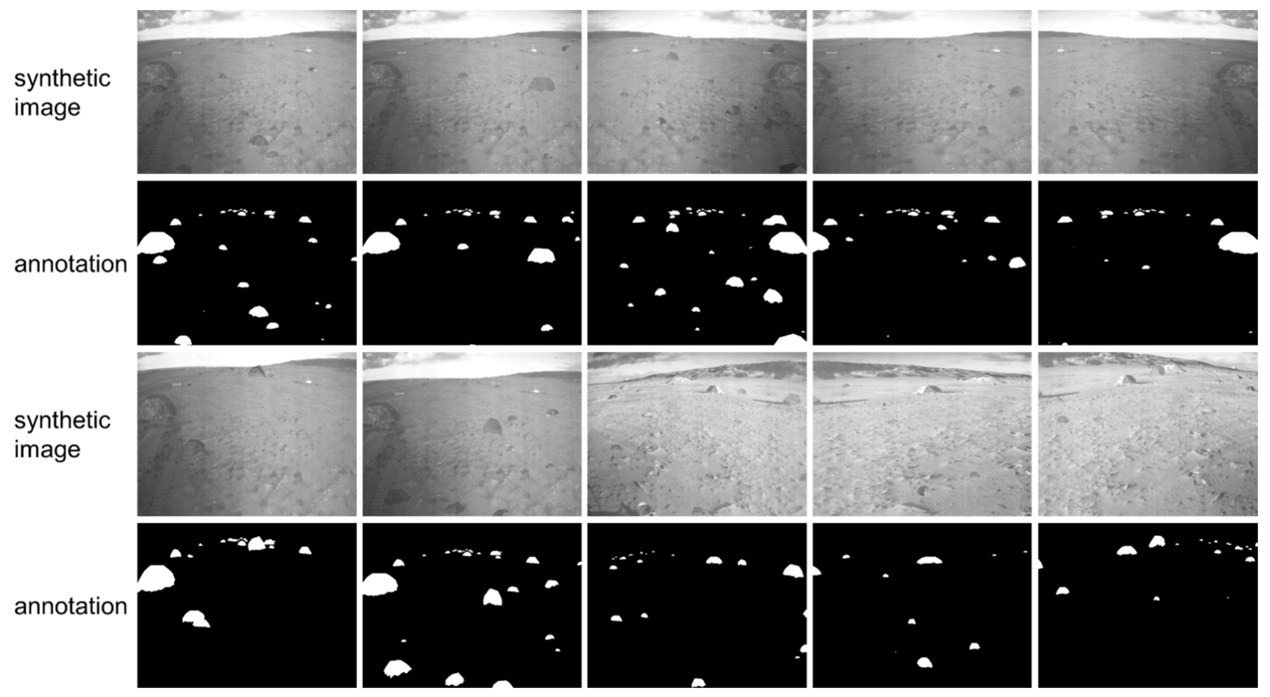
- Then, the synthetic algorithm utilizes these backgrounds and rock samples to generate the synthetic dataset. The synthetic dataset contains 14,000 synthetic images and corresponding annotations.
- (c)
- The orange solid round frame refers to the proposed rock segmentation network (NI-U-Net++). The blue dash arrow refers to the pre-training, which aims to achieve prior knowledge from the synthetic dataset.
- (d)
- The pre-training process eventually accomplishes the pre-trained weights of the NI-U-Net++, and these pre-trained weights refer to the prior knowledge from the synthetic dataset.
- (3)
- In the transfer-training process:
- (a)
- The purple ellipse with “Annotation-2” refers to the second manual annotation, which aims to produce some pixel-level annotations (see the green round frame with “Annotated visual dataset”). The “Annotated visual dataset” contains 183 real-life images and corresponding pixel-level annotations.
- (b)
- The green dash arrow refers to the transfer training, which aims to fine-tune the pre-trained weights to fit the “Annotated visual dataset”.
- (c)
- (iii–iii) The transfer-training process comes up with the final weights of the NI-U-Net++.
2.1. The Real-Life Visual Navigation Dataset for the Planetary Rovers
2.2. The Synthetic Dataset
- (1)
- The synthetic algorithm also prepares data for the pre-training process. Therefore, the materials utilized in the synthetic algorithm should come from the real-life images.
- (2)
- Another target is to generate images and annotations synchronously through the synthesis algorithm, thereby significantly reducing the cost of manual intervention.
- (3)
- The target is to ensure the diversity of the synthetic dataset. The pre-training dataset can determine the robustness and generalization ability of the segmentation framework for the navigation visions. The data diversity introduced through morphology, brightness, and contrast transformations are significantly important to the above end.
- (4)
- The embedded rock samples require further processing to simulate the visual comfortable images.
2.2.1. The Proposed Synthetic Algorithm
- i.
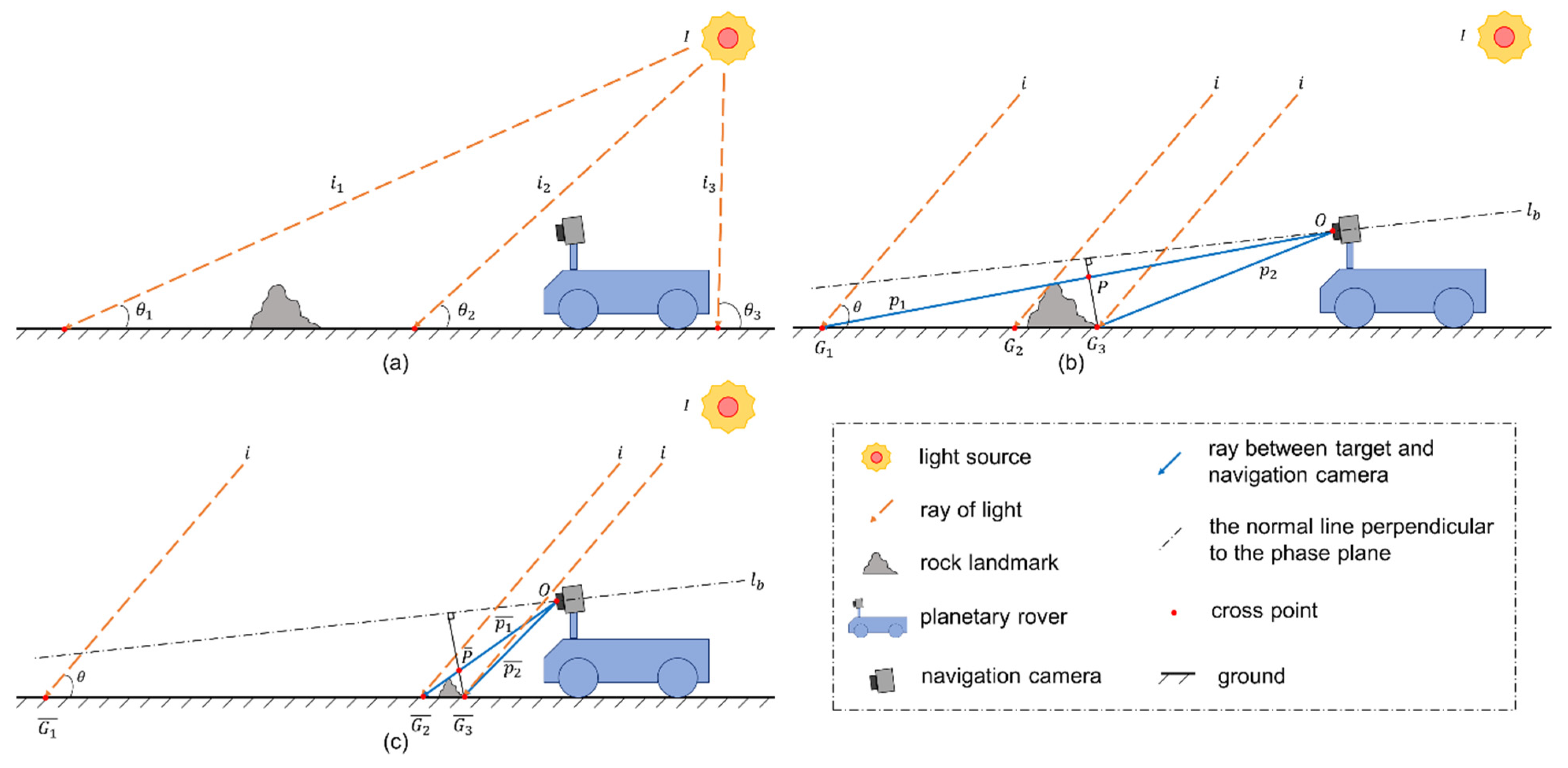
- The above discussion uses Equation (2) to achieve the desired illumination intensity, while is difficult to obtain from a grayscale image. However, the known information is the corresponding image grayscale value () and the area of . It is noteworthy that and appear in the same image region. This research assumes that the ratio () between the sum grayscale in and the area of can approximate the value of (see Equation (4)).However, Figure 2c shows another scenario. A pronounced difference between (Figure 2b) and (Figure 2c) comes from a smaller and closer rock landmark. Therefore, the difference () between and is located on (equivalent to ). It is noteworthy that is the ratio between the sum grayscale of and , whereas is the ratio between the sum grayscale of to (see Equation (5)).Substituting Equation (2) into Equation (5) can produce Equation (6), so is a value related to .
- ii.
- The optical properties of the object surface are complex (such as surface reflectance, refracting, and absorptivity), and they do not belong to the scope of this research. Here, we use a variable to pack all factors related to optical properties. Equation (7) depicts the grayscale change caused through the optical properties.
2.2.2. Implementation
- i.
- This research randomly picks up 35 images from the Katwijk dataset for “Annotation-1”. The number of 35 images is arbitrary; it needs to be large enough to get a sufficient dataset of rock annotations but not too large that it takes a long time to annotate the images. Furthermore, this research focuses on exploring a feasible framework so that the upper and lower limits of the image number in “Annotation-1” are not studied thoroughly.
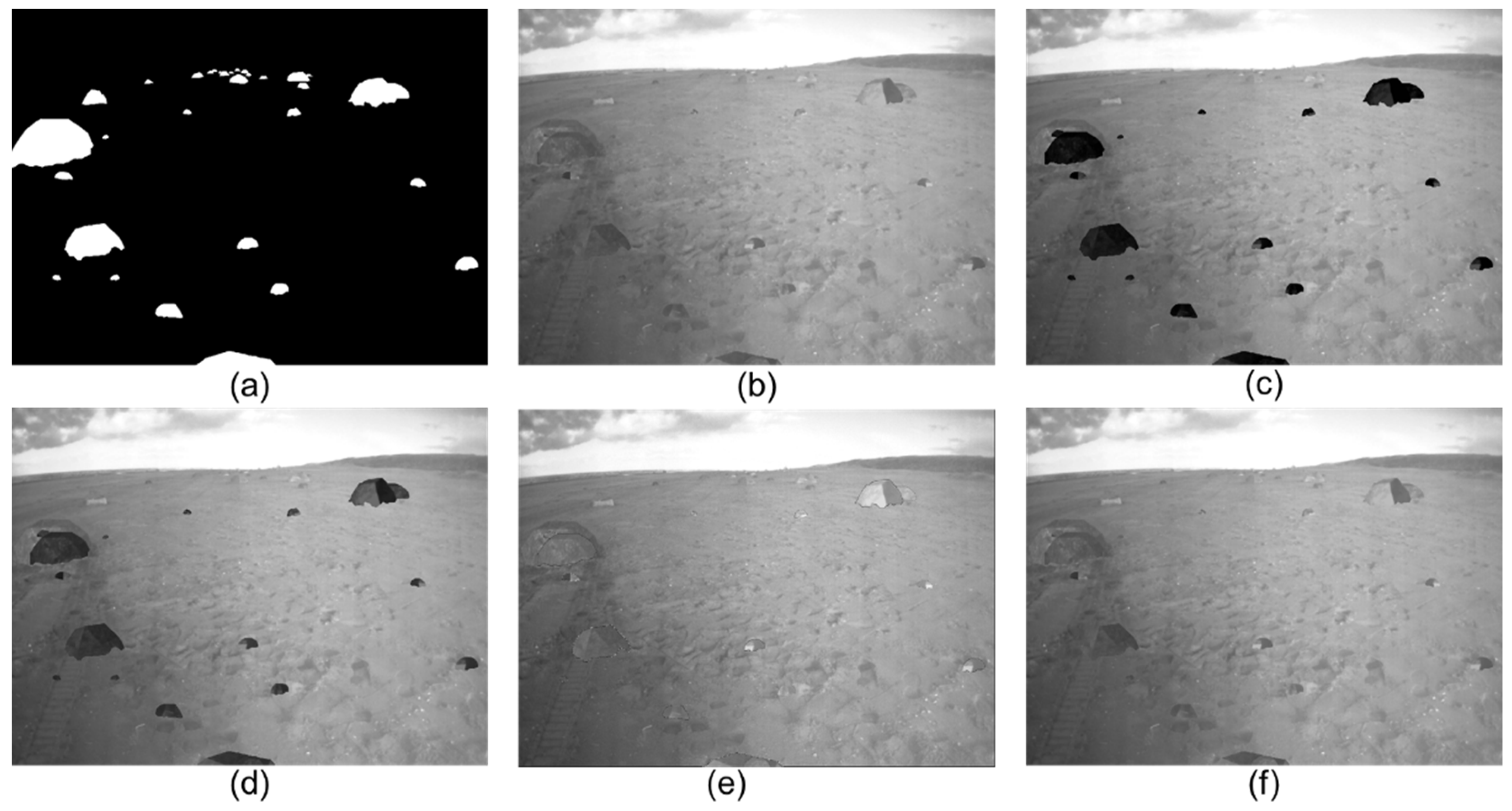
- ii.
- Then, the synthetic algorithm conducts the “Annotation-1” to these images (see Figure 3). The red mask refers to the rock sample, and the green masks refer to other rocks. It is noteworthy that each image only includes the largest rock in the rock samples. Before embedding into a new background, a morphological transformation is necessary to ensure the variant of the synthetic dataset. However, the enlarged morphological transformations can bring a significant resolution change if the rock sample is too small.
- iii.
- The algorithm also utilizes the images in “Annotation-1” as backgrounds for the synthetic algorithm. The annotation rule for “Annotation-1” is: if a rock cannot be identified with the three to six times enlargement, this research decides to abandon it as a part of the background.
- iv.
- The above three steps finish the data preparation for the synthetic algorithm. The refer to rock samples, and refer to backgrounds. Then, the algorithm conducts Algorithm 1 to generate the synthetic dataset.
- v.
- Morphological transformations can increase the number and diversity of the synthetic dataset. The morphological transformation schemes for rock samples () come from the combinations using mirror, flatten, narrowing, and zooming. The morphological transformation schemes for backgrounds () further include the adjustments of brightness, contrast, and sharpness.
- vi.
- Then, Algorithm 1 traverses each background with all to achieve the morphologically transformed images ( in Algorithm 1) (see row 3 and 4 in Algorithm 1). Meanwhile, the sky and ground segmentation model is applied to identify the ground pixels, and the rock samples are only embedded into the ground region. The sky and ground segmentation model comes from [57].
- vii.
- For each the synthetic algorithm embeds a random number of (see row 11 in Algorithm 1).
Algorithm 1: Synthetic algorithm Input: rock samples: rock = [rock1, rock2, …, rock35] practical sense: sense = [scene1, scene2, …, scene35] correction constant: C = [C1, C2, …, C11] scene augmentation: augscene = [s1, s2, …, s8] rock augmentation: augrock = [r1, r2, …, r9] Output: Synthetic dataset: img = [img1, img2, …, imgn] ![Mathematics 09 03048 i001]()
- viii.
- Each comes from a random selection from the rocks (). The algorithm also randomly selects a morphological transformation scheme () from . The algorithm conducts to , which results in a morphologically transformed rock () (see rows 9, 10, and 11 in Algorithm 1).
- ix.
- The algorithm adopts Equation (8), Equation (4), Table 2, and Equation (9) to achieve , , the correction constant for the corresponding (), and the grayscale values of the embedded rock () (see rows 12, 14, 15, and 16 in Algorithm 1). The further discussion of the values in Table 2 can be found in Appendix A.2.
- x.
- Finally, the synthetic images that correspond to the are saved as the synthetic dataset.

2.3. Proposed Rock Segmentation Network
2.4. The Pre-Training Process
- (i)
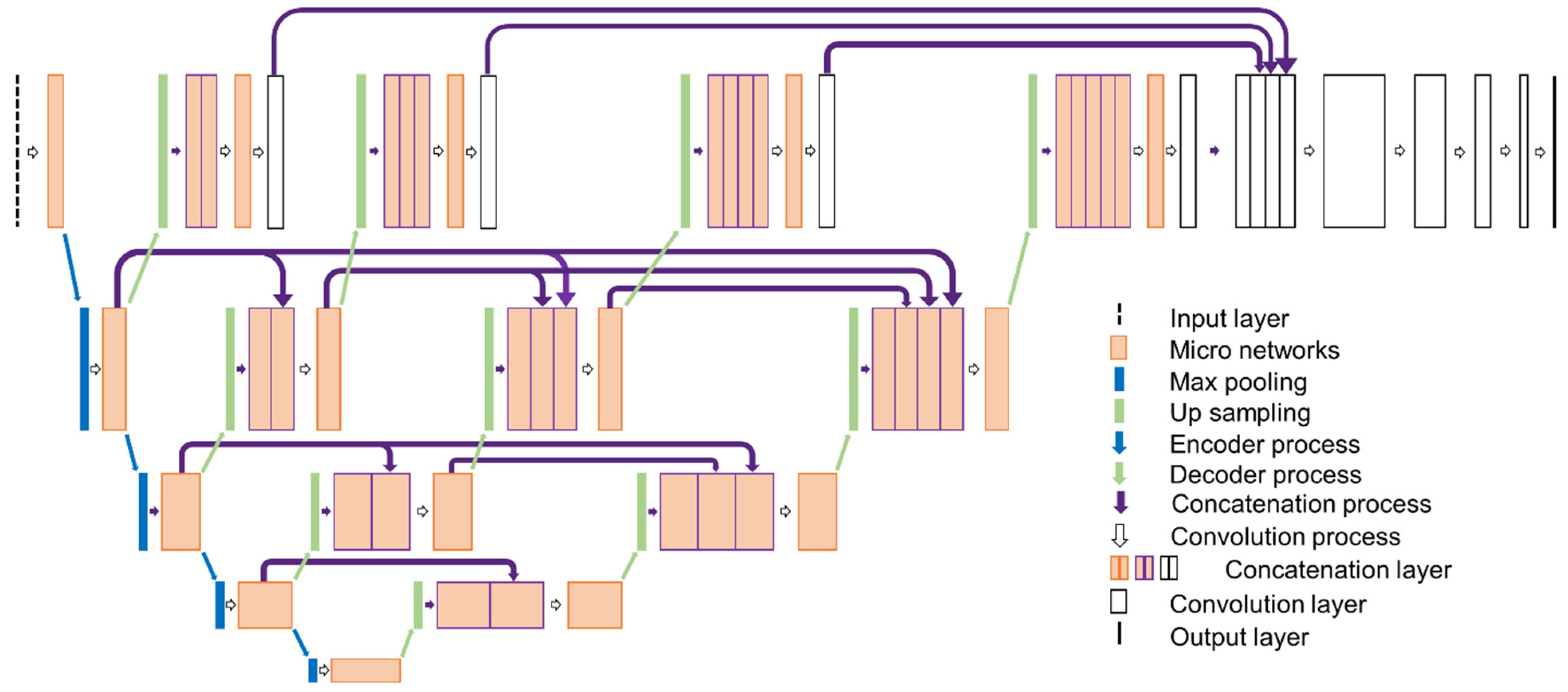
- U-Net is proposed by Ronneberger et al. [14], which is a very popular one-stage image segmentation network [60,61]. The applied U-Net references the high-starred implementations on GitHub [62,63]. The encoder of U-Net contains four downsampling layers, the decoder contains four upsampling layers, and the activation uses the “ReLU” function. The size of each convolution kernel is 3 × 3.
- (ii)
- (iii)
- The NI-U-Net [57] shares the same architecture as the sky and ground segmentation network used in Section 2.2. NI-U-Net only contains a single U-shaped encoder-decoder design, and the micro-networks have also been applied.
- (iv)
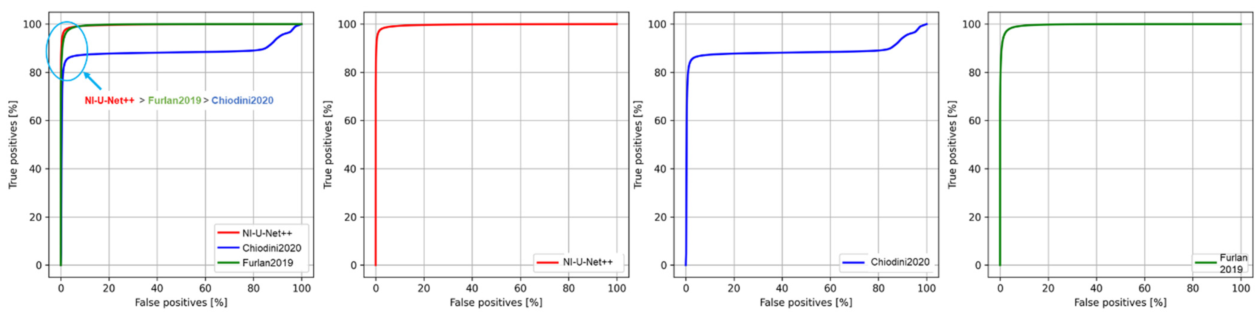
- Furlan et al. proposed a deeplabv3plus-based rock segmentation solution in 2019, and the implementation of Furlan2019 referenced the study in [43].
- (v)
- Chiodini et al. proposed a fully convolutional network-based rock segmentation solution in 2020; the implementation of Chiodini2020 referenced the study in [44].
2.5. The Transfer-Training Process
- (1)
- “Annotation-2” randomly re-selects 150 images from the Katwijk dataset.
- (2)
- “Annotation-2” performs pixel-level annotations on these images.
- (3)
- The images annotated in “Annotation-1” can also be used for the transfer-training process, so “Annotation-2” merges 35 images in “Annotation-1” with the 150 images. It is noteworthy that there are two duplicate images, so the final number of images for “Annotation-2” is 183 images (The 183 images are only about 8% of the Katwijk dataset)
- (4)
- “Annotation-2” uses data augmentation to simulate possible situations for the planetary rover operations. For example, rotations simulate the pose changes, brightness changes simulate changes in illumination conditions, and contrast changes simulate changes in imaging conditions. The data augmentation eventually achieves about 4000 images.
3. Results and Discussion
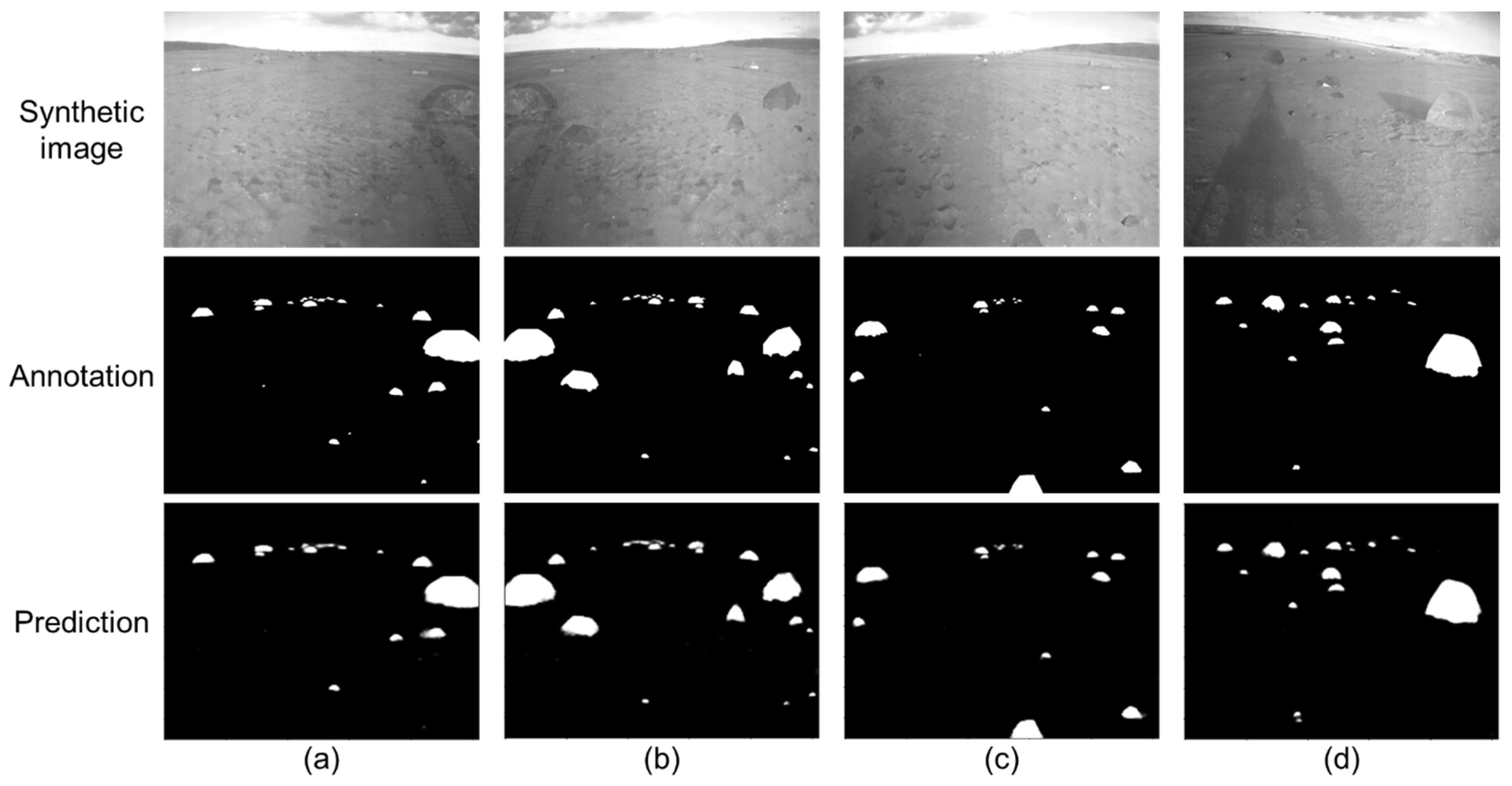
3.1. The Results of the Proposed Synthetic Algorithm
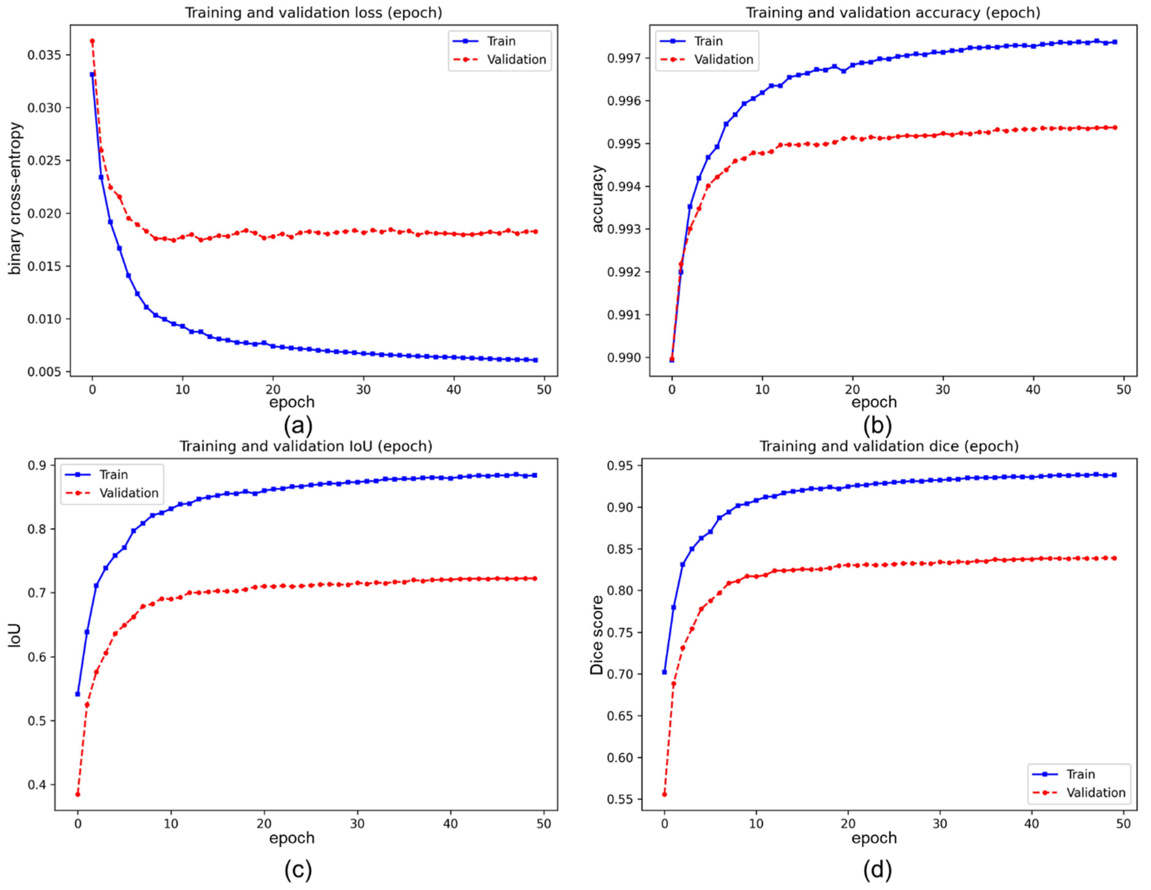
3.2. The Results of the Pre-Training Process
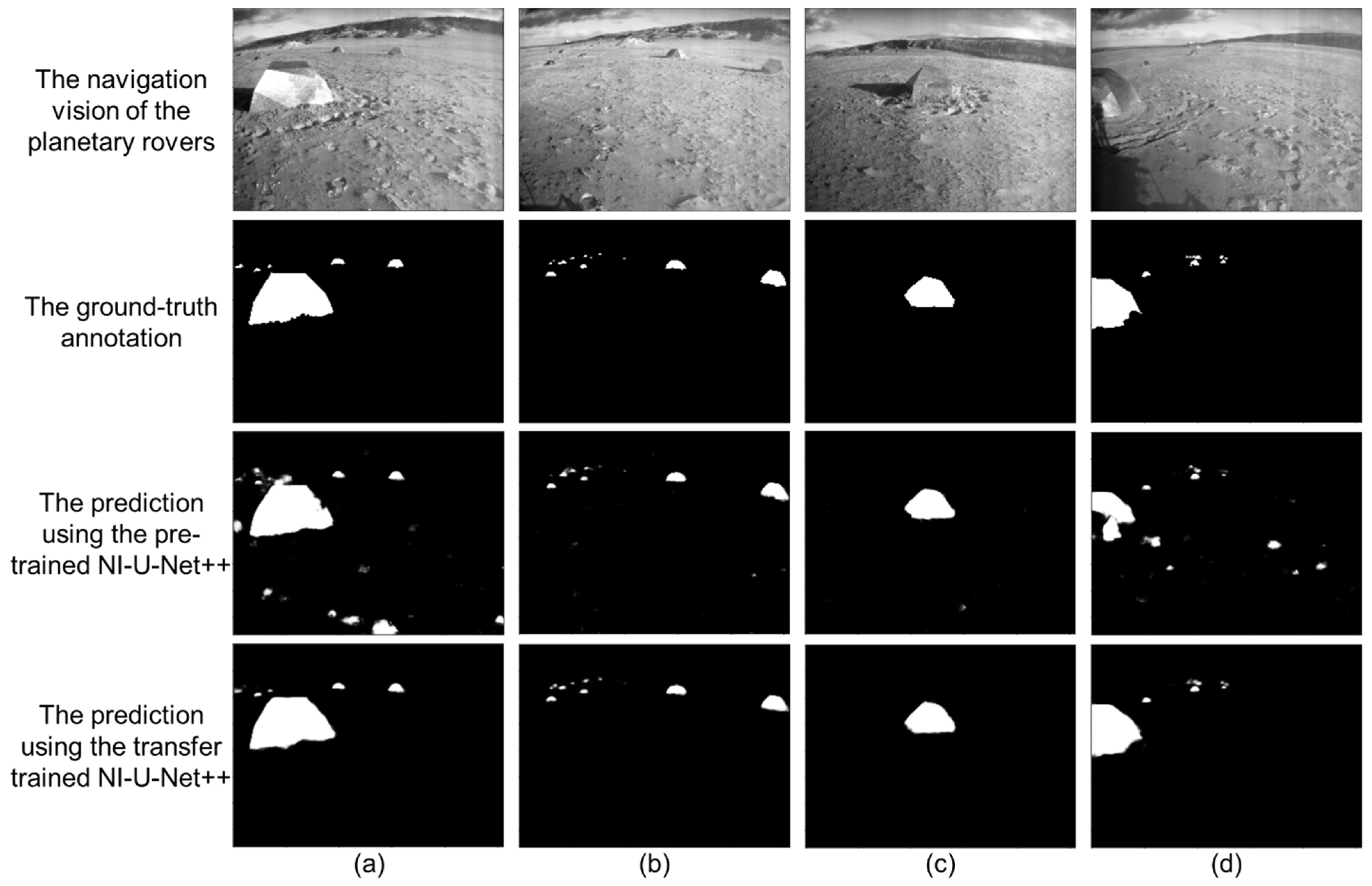
3.3. The Results of the Transfer-Training Process
4. Conclusions and Future Works
Supplementary Materials
Author Contributions
Funding
Data Availability Statement
Acknowledgments
Conflicts of Interest
Nomenclature
| , , , | Formal parameters. |
| Light source. | |
| , | Rays of light. |
| Horizontal ground. | |
| , , , | Angles between the corresponding ray of the Light and the horizontal ground. |
| The density of rays in the unit ground area. | |
| Light intensity. | |
| Area of a ground region. | |
| , | The boundary rays between object and camera. |
| The normal line perpendicular to the phase plane. | |
| The area between and cross-points. | |
| , | Cross points on the ground. |
| Cross point between and . | |
| The origin of image plane. | |
| The light intensity in the area between and cross-points in the sketch. | |
| Abstracted value of the optical properties. | |
| A variable to pack all factors related to optical properties. | |
| An approximate value of . | |
| The target (rocks in this research) in the sketch. | |
| Coordinate. | |
| Grayscale value at coordinate . | |
| The number of pixels in a specific region. | |
| The difference between and . | |
| The area between and cross-points. | |
| An implicit function to correlate the optical properties and image grayscales. | |
| The averaged grayscale value for the corresponding image area. | |
| A set of the grayscale values for the corresponding image area. | |
| A set of the differential values between and (only related to the coordinates). | |
| The constants to correct from . | |
| An approximation of using the proposed synthetic algorithm. |
Appendix A
Appendix A.1. Further Details of the Related Studies

| Reference | Category in Table 1 1 | Results 2 |
|---|---|---|
| [30] | i | Only the qualitative segmentation results. |
| [31] | i | Only the qualitative segmentation results. |
| [32] | i | Only the qualitative segmentation results. |
| [4] | ii | Fit error = 1.504~114.934. |
| [5] | ii and iii | Only the qualitative segmentation results. |
| [33] | ii | Only the qualitative segmentation results. |
| [34] | ii | (1) Average precision = 89% (the center matching method); (2) Average precision = 87% (the overlap method); (3) Average precision ≥ 90% = 83 images. |
| [35] | ii and v | (1) Standard deviation of recall = 0.2–0.3; (2) Standard deviation of precision = 0.2–0.3; (3) Recall and precision are modestly improved. |
| [36] | ii | Only the qualitative segmentation results. |
| [37] | iii | Only the qualitative segmentation results. |
| [38] | iii | (1) RMS error (X) = 0.22–0.93 (HiRISE pixel), RMS error (Y) = 0.22–0.97 (HiRISE pixel); (2) RMS error (X) = 0.23–0.70 (HiRISE pixel), RMS error (Y) = 0.23–0.89 (HiRISE pixel). |
| [32] | iv | CPU time (seconds): 0.2214–0.7484 (MAD); 0.1966–0.6955 (LMedsq); 0.5994–2.2033 (IKOSE); 0.2931–0.9633 (PDIMSE); 0.0380–0.1238 (RANSAC); 106.4747–236.2487 (RECON). |
| [39] | iv | (1) Processing time: 2–3 s for 256 * 256 images; 20–45 s for 640 * 480 images (2) Only the qualitative segmentation results. |
| [40] | iv | Medium rock match is successful (up to 26 m). |
| [41] | iv | The proposed method is robust and efficient for small- and large-scale rock detection. |
| [8] | v | A survey for terrain classification (including rock segmentation). |
| [27] | v | (1) Pixel-wise accuracy = 99.69% (background); 97.89% (sand); 89.33% (rock); 96.33% (gravel); 89.73% (bedrock). (2) Mean intersection-over-union (mIoU) = 0.9459. |
| [28] | v | (1) Accuracy = 76.2% (derivable terrain comprising sand, bedrock, and loose rock); (2) Accuracy = 89.2% (embedded pointy rocks). |
| [42] | v | mIoU = 0.93; recall = 96%; frame rate = 116 frame per second |
| [43] | v | F-score = 78.5% |
| [44] | v | Accuracy = 90~96%; IoU = 0.21~0.58. |
Appendix A.2. The Experiments of the Values in Table 2

Appendix A.3. Qualitative Examples of the Proposed Synthetic Dataset

Appendix A.4. Pairwise Comparisons between Proposed NI-U-Net++ and Related Studies
- i.
- ii.
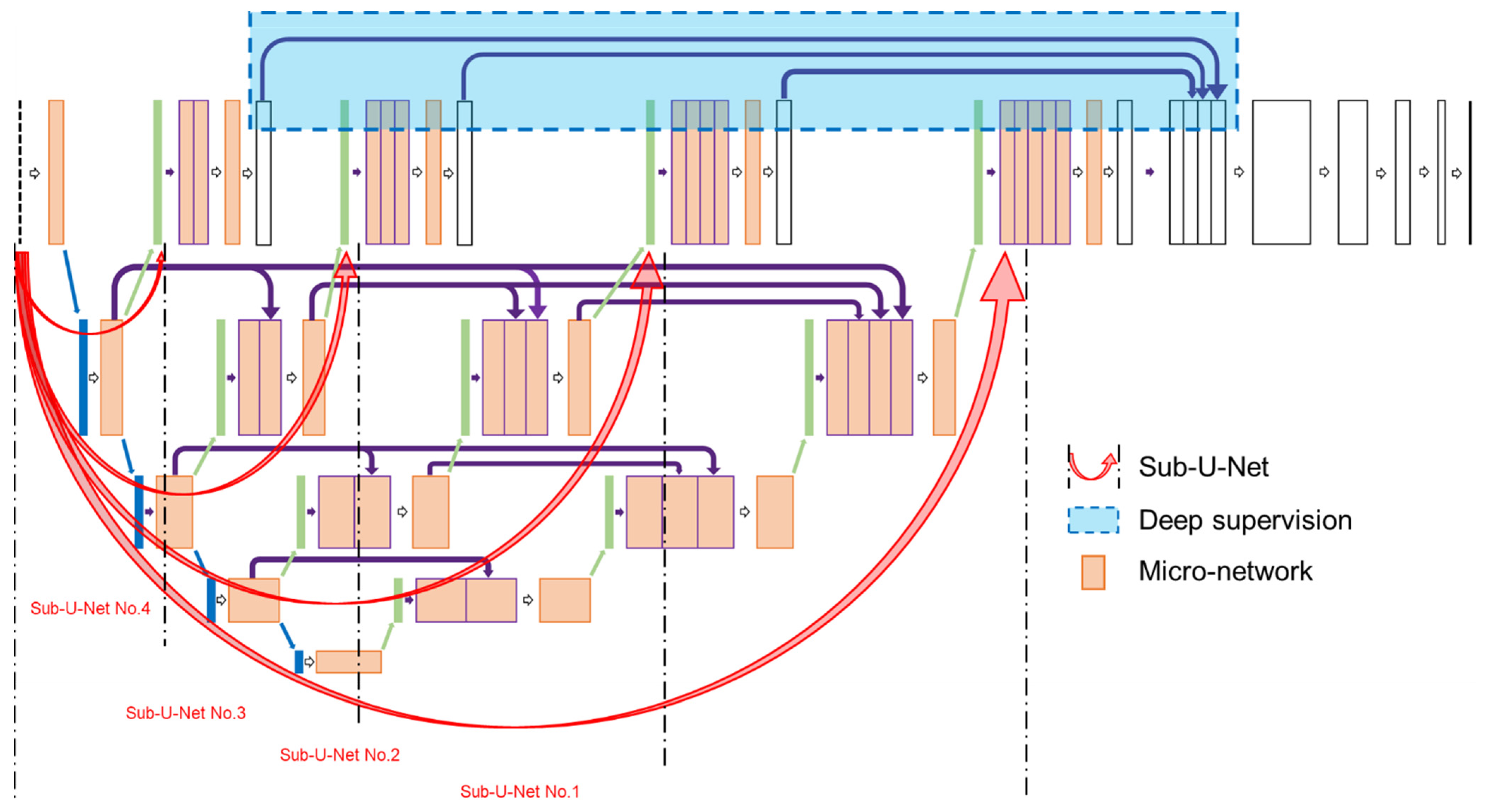
- NI-U-Net++ with U-Net++ [15]:
- a.
- U-Net++ also has four sub-U-Nets as in the NI-U-Net++.
- b.
- U-Net++ also has the deep supervision as in the NI-U-Net++.
- c.
- However, the U-Net++ applies the 3 × 3 convolution layer and “Relu” activation as in U-Net instead of the micro-network in NI-U-Net++.
- iii.
- NI-U-Net++ with NI-U-Net [57]:
- a.
- NI-U-Net only has the “Sub-U-Net No. 1”. Therefore, the compression ratio is constant at a high level.
- b.
- NI-U-Net has not deep supervision design.
- c.
- NI-U-Net utilizes the same micro-network as in NI-U-Net++.

Appendix A.5. Additional Results of the Pre-Training Process
| Networks | Dice Score | ||
|---|---|---|---|
| Train | Valid | Test | |
| U-Net | 0.9158 | 0.9040 | 0.9044 |
| U-Net++ | 0.9574 | 0.9344 | 0.9352 |
| NI-U-Net | 0.9644 | 0.9313 | 0.9316 |
| NI-U-Net++ | 0.9588 | 0.9458 | 0.9469 |


| Number 1 (Images) | Loss | Accuracy | IoU | Dice Score | ||||||||
|---|---|---|---|---|---|---|---|---|---|---|---|---|
| Train | Valid | Test | Train | Valid | Test | Train | Valid | Test | Train | Valid | Test | |
| 7000 | 0.0137 | 0.0189 | 0.0199 | 99.49% | 99.39% | 99.37% | 0.9164 | 0.8919 | 0.8876 | 0.9564 | 0.9429 | 0.9405 |
| 1000 | 0.0273 | 0.0618 | 0.0580 | 99.53% | 99.02% | 99.03% | 0.9175 | 0.8374 | 0.8389 | 0.9570 | 0.9115 | 0.9124 |
Appendix A.6. Additional Results of the Transfer-Training Process


References
- Privitera, C.M.; Stark, L.W. Human-vision-based selection of image processing algorithms for planetary exploration. IEEE Trans. Image Process. 2003, 12, 917–923. [Google Scholar] [CrossRef] [PubMed]
- Kim, W.S.; Diaz-Calderon, A.; Peters, S.F.; Carsten, J.L.; Leger, C. Onboard centralized frame tree database for intelligent space operations of the Mars Science Laboratory rover. IEEE Trans. Cybern. 2014, 44, 2109–2121. [Google Scholar] [CrossRef]
- Gao, Y.; Chien, S. Review on space robotics: Toward top-level science through space exploration. Sci. Robot. 2017, 2, eaan5074. [Google Scholar] [CrossRef] [Green Version]
- Castano, R.; Estlin, T.; Gaines, D.; Chouinard, C.; Bornstein, B.; Anderson, R.C.; Burl, M.; Thompson, D.; Castano, A.; Judd, M. Onboard autonomous rover science. In Proceedings of the 2007 IEEE Aerospace Conference, Big Sky, MT, USA, 3–10 March 2007; pp. 1–13. [Google Scholar]
- Estlin, T.A.; Bornstein, B.J.; Gaines, D.M.; Anderson, R.C.; Thompson, D.R.; Burl, M.; Castaño, R.; Judd, M. AEGIS automated science targeting for the MER opportunity rover. ACM Trans. Intell. Syst. Technol. 2012, 3, 1–19. [Google Scholar] [CrossRef]
- Otsu, K.; Ono, M.; Fuchs, T.J.; Baldwin, I.; Kubota, T. Autonomous terrain classification with co- and self-training approach. IEEE Robot. Autom. Lett. 2016, 1, 814–819. [Google Scholar] [CrossRef]
- Swan, R.M.; Atha, D.; Leopold, H.A.; Gildner, M.; Oij, S.; Chiu, C.; Ono, M. AI4MARS: A dataset for terrain-aware autonomous driving on Mars. In Proceedings of the 2021 IEEE/CVF Conference on Computer Vision and Pattern Recognition Workshops (CVPRW), Nashville, TN, USA, 19–25 June 2021. [Google Scholar]
- Gao, Y.; Spiteri, C.; Pham, M.-T.; Al-Milli, S. A survey on recent object detection techniques useful for monocular vision-based planetary terrain classification. Robot. Auton. Syst. 2014, 62, 151–167. [Google Scholar] [CrossRef]
- Minaee, S.; Boykov, Y.; Porikli, F.; Plaza, A.; Kehtarnavaz, N.; Terzopoulos, D. Image segmentation using deep learning: A survey. IEEE Trans. Pattern Anal. Mach. Intell. 2020, 1–22. [Google Scholar] [CrossRef]
- Liu, D.; Bober, M.; Kittler, J. Visual semantic information pursuit: A survey. IEEE Trans. Pattern Anal. Mach. Intell. 2021, 43, 1404–1422. [Google Scholar] [CrossRef] [Green Version]
- Zoller, T.; Buhmann, J.M. Robust image segmentation using resampling and shape constraints. IEEE Trans. Pattern Anal. Mach. Intell. 2007, 29, 1147–1164. [Google Scholar] [CrossRef]
- Alpert, S.; Galun, M.; Brandt, A.; Basri, R. Image segmentation by probabilistic bottom-up aggregation and cue integration. IEEE Trans. Pattern Anal. Mach. Intell. 2012, 34, 315–327. [Google Scholar] [CrossRef] [Green Version]
- Saltzer, J.H.; Reed, D.P.; Clark, D.D. End-to-end arguments in system design. ACM Trans. Comput. Syst. 1984, 2, 277–288. [Google Scholar] [CrossRef] [Green Version]
- Ronneberger, O.; Fischer, P.; Brox, T. U-Net: Convolutional networks for biomedical image segmentation. In Lecture Notes in Computer Science (Including Subseries Lecture Notes in Artificial Intelligence and Lecture Notes in Bioinformatics); Springer: Berlin/Heidelberg, Germany, 2015; Volume 9351, pp. 234–241. ISBN 9783319245737. [Google Scholar]
- Zhou, Z.; Rahman Siddiquee, M.M.; Tajbakhsh, N.; Liang, J. Unet++: A nested u-net architecture for medical image segmentation. In Lecture Notes in Computer Science (Including Subseries Lecture Notes in Artificial Intelligence and Lecture Notes in Bioinformatics); Springer: Berlin/Heidelberg, Germany, 2018; Volume 11045, pp. 3–11. [Google Scholar] [CrossRef] [Green Version]
- Chen, L.-C.; Papandreou, G.; Kokkinos, I.; Murphy, K.; Yuille, A.L. Semantic image segmentation with deep convolutional nets and fully connected CRFs. arXiv 2014, arXiv:1412.7062. [Google Scholar]
- Liu, W.; Anguelov, D.; Erhan, D.; Szegedy, C.; Reed, S.; Fu, C.-Y.; Berg, A.C. SSD: Single shot multibox detector. In Lecture Notes in Computer Science (Including Subseries Lecture Notes in Artificial Intelligence and Lecture Notes in Bioinformatics); Springer: Berlin/Heidelberg, Germany, 2016; Volume 9905, pp. 21–37. ISBN 9783319464473. [Google Scholar]
- Gupta, S.; Girshick, R.; Arbeláez, P.; Malik, J. Learning rich features FROM RGB-D images for object detection and segmentation. In Lecture Notes in Computer Science; Springer: Berlin/Heidelberg, Germany, 2014; Volume 8695, pp. 345–360. ISBN 9783319105833. [Google Scholar]
- Hariharan, B.; Arbeláez, P.; Girshick, R.; Malik, J. Simultaneous detection and segmentation. In Lecture Notes in Computer Science; Springer: Berlin/Heidelberg, Germany, 2014; Volume 8695, pp. 297–312. ISBN 9783319105833. [Google Scholar]
- He, K.; Gkioxari, G.; Dollár, P.; Girshick, R. Mask R-CNN. IEEE Trans. Pattern Anal. Mach. Intell. 2017, 42, 386–397. [Google Scholar] [CrossRef]
- Dewan, A.; Oliveira, G.L.; Burgard, W. Deep semantic classification for 3D LiDAR data. In Proceedings of the 2017 IEEE/RSJ International Conference on Intelligent Robots and Systems (IROS), Vancouver, BC, Canada, 24–28 September 2017; Volume 2017, pp. 3544–3549. [Google Scholar]
- Badrinarayanan, V.; Kendall, A.; Cipolla, R. SegNet: A deep convolutional encoder-decoder architecture for image segmentation. IEEE Trans. Pattern Anal. Mach. Intell. 2017, 39, 2481–2495. [Google Scholar] [CrossRef] [PubMed]
- Teichmann, M.; Weber, M.; Zollner, M.; Cipolla, R.; Urtasun, R. MultiNet: Real-time joint semantic reasoning for autonomous driving. In Proceedings of the 2018 IEEE Intelligent Vehicles Symposium (IV), Suzhou, China, 26–30 June 2018; Volume 2018, pp. 1013–1020. [Google Scholar]
- Wu, B.; Wan, A.; Yue, X.; Keutzer, K. SqueezeSeg: Convolutional neural nets with recurrent CRF for real-time road-object segmentation from 3D LiDAR point cloud. In Proceedings of the 2018 IEEE International Conference on Robotics and Automation (ICRA), Brisbane, Australia, 21–25 May 2018; pp. 1887–1893. [Google Scholar]
- Busquets, D.; Sierra, C.; López de Màntaras, R. A multiagent approach to qualitative landmark-based navigation. Auton. Robots 2003, 15, 129–154. [Google Scholar] [CrossRef]
- Kovács, G.; Kunii, Y.; Maeda, T.; Hashimoto, H. Saliency and spatial information-based landmark selection for mobile robot navigation in natural environments. Adv. Robot. 2019, 33, 520–535. [Google Scholar] [CrossRef]
- Zhou, R.; Ding, L.; Gao, H.; Feng, W.; Deng, Z.; Li, N. Mapping for planetary rovers from terramechanics perspective. In Proceedings of the 2019 IEEE/RSJ International Conference on Intelligent Robots and Systems (IROS), Macau, China, 3–8 November 2019; pp. 1869–1874. [Google Scholar]
- Ono, M.; Fuchs, T.J.; Steffy, A.; Maimone, M.; Jeng, Y. Risk-aware planetary rover operation: Autonomous terrain classification and path planning. In Proceedings of the 2015 IEEE Aerospace Conference, Big Sky, MT, USA, 7–14 March 2015; pp. 1–10. [Google Scholar]
- Zhou, F.; Arvidson, R.E.; Bennett, K.; Trease, B.; Lindemann, R.; Bellutta, P.; Iagnemma, K.; Senatore, C. Simulations of Mars rover traverses. J. Field Robot. 2014, 31, 141–160. [Google Scholar] [CrossRef]
- Pedersen, L. Science target assessment for Mars rover instrument deployment. In Proceedings of the IEEE/RSJ International Conference on Intelligent Robots and System, Lausanne, Switzerland, 30 September–4 October 2002; Volume 1, pp. 817–822. [Google Scholar]
- Di, K.; Yue, Z.; Liu, Z.; Wang, S. Automated rock detection and shape analysis from mars rover imagery and 3D point cloud data. J. Earth Sci. 2013, 24, 125–135. [Google Scholar] [CrossRef]
- Xiao, X.; Cui, H.; Tian, Y. Robust plane fitting algorithm for landing hazard detection. IEEE Trans. Aerosp. Electron. Syst. 2015, 51, 2864–2875. [Google Scholar] [CrossRef]
- Dunlop, H.; Thompson, D.R.; Wettergreen, D. Multi-scale features for detection and segmentation of rocks in Mars images. In Proceedings of the 2007 IEEE Conference on Computer Vision and Pattern Recognition, Minneapolis, MN, USA, 18–23 June 2007; pp. 1–7. [Google Scholar]
- Castano, R.; Judd, M.; Estlin, T.; Anderson, R.C.; Gaines, D.; Castano, A.; Bornstein, B.; Stough, T.; Wagstaff, K. Current results from a rover science data analysis system. In Proceedings of the 2005 IEEE Aerospace Conference, Big Sky, MT, USA, 5–12 March 2005; Volume 2005, pp. 356–365. [Google Scholar]
- Castano, R.; Mann, T.; Mjolsness, E. Texture analysis for Mars rover images. In Applications of Digital Image Processing XXII; Tescher, A.G., Ed.; Society of Photo-optical Instrumentation Engineers: Bellingham, WA, USA, 1999; Volume 3808, pp. 162–173. [Google Scholar]
- Burl, M.C.; Thompson, D.R.; DeGranville, C.; Bornstein, B.J. Rockster: Onboard rock segmentation through edge regrouping. J. Aerosp. Inf. Syst. 2016, 13, 329–342. [Google Scholar] [CrossRef]
- Castafio, R.; Anderson, R.C.; Estlin, T.; DeCoste, D.; Fisher, F.; Gaines, D.; Mazzoni, D.; Judd, M. Rover traverse science for increased mission science return. In Proceedings of the 2003 IEEE Aerospace Conference Proceedings, Big Sky, MT, USA, 8–15 March 2003; Volume 8, pp. 8_3629–8_3636. Available online: https://ieeexplore.ieee.org/document/1235546 (accessed on 26 November 2021).
- Di, K.; Liu, Z.; Yue, Z. Mars rover localization based on feature matching between ground and orbital imagery. Photogramm. Eng. Remote Sens. 2011, 77, 781–791. [Google Scholar] [CrossRef]
- Gulick, V.C.; Morris, R.L.; Ruzon, M.A.; Roush, T.L. Autonomous image analyses during the 1999 Marsokhod rover field test. J. Geophys. Res. Planets 2001, 106, 7745–7763. [Google Scholar] [CrossRef]
- Li, R.; Di, K.; Howard, A.B.; Matthies, L.; Wang, J.; Agarwal, S. Rock modeling and matching for autonomous long-range Mars rover localization. J. Field Robot. 2007, 24, 187–203. [Google Scholar] [CrossRef]
- Yang, J.; Kang, Z. A gradient-region constrained level set method for autonomous rock detection from Mars rover image. Int. Arch. Photogramm. Remote Sens. Spat. Inf. Sci. ISPRS Arch. 2019, 42, 1479–1485. [Google Scholar] [CrossRef]
- Zhou, R.; Feng, W.; Yang, H.; Gao, H.; Li, N.; Deng, Z.; Ding, L. Predicting terrain mechanical properties in sight for planetary rovers with semantic clues. arXiv 2020, arXiv:2011.01872. [Google Scholar]
- Furlán, F.; Rubio, E.; Sossa, H.; Ponce, V. Rock detection in a Mars-like environment using a CNN. In Lecture Notes in Computer Science (Including Subseries Lecture Notes in Artificial Intelligence and Lecture Notes in Bioinformatics); Springer: Berlin/Heidelberg, Germany, 2019; Volume 11524, pp. 149–158. [Google Scholar] [CrossRef]
- Chiodini, S.; Torresin, L.; Pertile, M.; Debei, S. Evaluation of 3D CNN semantic mapping for rover navigation. In Proceedings of the 2020 IEEE International Workshop on Metrology for AeroSpace, Pisa, Italy, 22 June–5 July 2020; pp. 32–36. [Google Scholar] [CrossRef]
- Pessia, R. Artificial Lunar Landscape Dataset. Available online: https://www.kaggle.com/romainpessia/artificial-lunar-rocky-landscape-dataset (accessed on 22 June 2021).
- Bonechi, S.; Bianchini, M.; Scarselli, F.; Andreini, P. Weak supervision for generating pixel–level annotations in scene text segmentation. Pattern Recognit. Lett. 2020, 138, 1–7. [Google Scholar] [CrossRef]
- Nalepa, J.; Myller, M.; Kawulok, M. Transfer learning for segmenting dimensionally reduced hyperspectral images. IEEE Geosci. Remote Sens. Lett. 2020, 17, 1228–1232. [Google Scholar] [CrossRef] [Green Version]
- Li, J.; Zhang, L.; Wu, Z.; Ling, Z.; Cao, X.; Guo, K.; Yan, F. Autonomous Martian rock image classification based on transfer deep learning methods. Earth Sci. Inform. 2020, 13, 951–963. [Google Scholar] [CrossRef]
- Hewitt, R.A.; Boukas, E.; Azkarate, M.; Pagnamenta, M.; Marshall, J.A.; Gasteratos, A.; Visentin, G. The Katwijk beach planetary rover dataset. Int. J. Robot. Res. 2018, 37, 3–12. [Google Scholar] [CrossRef] [Green Version]
- Sánchez-Ibánez, J.R.; Pérez-del-Pulgar, C.J.; Azkarate, M.; Gerdes, L.; García-Cerezo, A. Dynamic path planning for reconfigurable rovers using a multi-layered grid. Eng. Appl. Artif. Intell. 2019, 86, 32–42. [Google Scholar] [CrossRef] [Green Version]
- Gerdes, L.; Azkarate, M.; Sánchez-Ibáñez, J.R.; Joudrier, L.; Perez-del-Pulgar, C.J. Efficient autonomous navigation for planetary rovers with limited resources. J. Field Robot. 2020, 37, 1153–1170. [Google Scholar] [CrossRef]
- Furlán, F.; Rubio, E.; Sossa, H.; Ponce, V. CNN based detectors on planetary environments: A performance evaluation. Front. Neurorobot. 2020, 14, 1–9. [Google Scholar] [CrossRef]
- Meyer, L.; Smíšek, M.; Fontan Villacampa, A.; Oliva Maza, L.; Medina, D.; Schuster, M.J.; Steidle, F.; Vayugundla, M.; Müller, M.G.; Rebele, B.; et al. The MADMAX data set for visual-inertial rover navigation on Mars. J. Field Robot. 2021, 38, 833–853. [Google Scholar] [CrossRef]
- Lamarre, O.; Limoyo, O.; Marić, F.; Kelly, J. The Canadian planetary emulation terrain energy-aware rover navigation dataset. Int. J. Robot. Res. 2020, 39, 641–650. [Google Scholar] [CrossRef]
- NASA. NASA Science Mars Exploration Program. Available online: https://mars.nasa.gov/mars2020/multimedia/raw-images/ (accessed on 29 May 2021).
- Pan, S.J.; Yang, Q. A survey on transfer learning. IEEE Trans. Knowl. Data Eng. 2010, 22, 1345–1359. [Google Scholar] [CrossRef]
- Kuang, B.; Rana, Z.A.; Zhao, Y. Sky and ground segmentation in the navigation visions of the planetary rovers. Sensors 2021, 21, 6996. [Google Scholar] [CrossRef] [PubMed]
- Lin, M.; Chen, Q.; Yan, S. Network in Network. In Proceedings of the 2nd International Conference on Learning Representations ICLR 2014, Banff, AB, Canada, 14–16 April 2014; pp. 1–10. [Google Scholar]
- Gurita, A.; Mocanu, I.G. Image segmentation using encoder-decoder with deformable convolutions. Sensors 2021, 21, 1570. [Google Scholar] [CrossRef]
- Marcinkiewicz, M.; Nalepa, J.; Lorenzo, P.R.; Dudzik, W.; Mrukwa, G. Segmenting brain tumors from MRI using cascaded multi-modal U-nets. In International MICCAI Brainleison Workshop; Springer: Berlin/Heidelberg, Germany, 2019; pp. 13–24. [Google Scholar]
- Tarasiewicz, T.; Nalepa, J.; Kawulok, M. Skinny: A lightweight U-net for skin detection and segmentation. In Proceedings of the 2020 IEEE International Conference on Image Processing (ICIP), Abu Dhabi, United Arab Emirates, 25–28 October 2020; pp. 2386–2390. [Google Scholar]
- Zhixuhao. Unet. Available online: https://github.com/zhixuhao/unet (accessed on 23 July 2021).
- Mulesial. Pytorch-UNet. Available online: https://github.com/milesial/Pytorch-UNet (accessed on 23 July 2021).
- 4uiiurz1. Pytorch-Nested-Unet. Available online: https://github.com/4uiiurz1/pytorch-nested-unet (accessed on 26 November 2021).
- Lin, C.H.; Kong, C.; Lucey, S. Learning efficient point cloud generation for dense 3D object reconstruction. In Proceedings of the 32nd AAAI Conference on Artificial Intelligence, New Orleans, LA, USA, 2–7 February 2018; pp. 7114–7121. [Google Scholar]
- Zuo, J.; Xu, G.; Fu, K.; Sun, X.; Sun, H. Aircraft type recognition based on segmentation with deep convolutional neural networks. IEEE Geosci. Remote Sens. Lett. 2018, 15, 282–286. [Google Scholar] [CrossRef]


| Category 1 | Explanation | Machine Learning-Based | Reference Index 2 |
|---|---|---|---|
| i | 3D point cloud | No | [30,31,32] |
| ii | Edge-based method | No (except [33]) | [4,5,33,34,35,36] |
| iii | Outstanding rocks | No | [5,37,38] |
| iv | Other non-machine learning studies | No | [32,39,40,41] |
| v | Machine learning studies | Yes | [8,27,28,35,42,43,44] |
| Conditions | Value 1 |
|---|---|
| 0 | |
| 5 | |
| 10 | |
| 15 | |
| 20 | |
| 25 | |
| 30 | |
| 35 | |
| 40 | |
| 45 | |
| 50 |
| Hyperparameter | Setting | Hyperparameter | Setting |
|---|---|---|---|
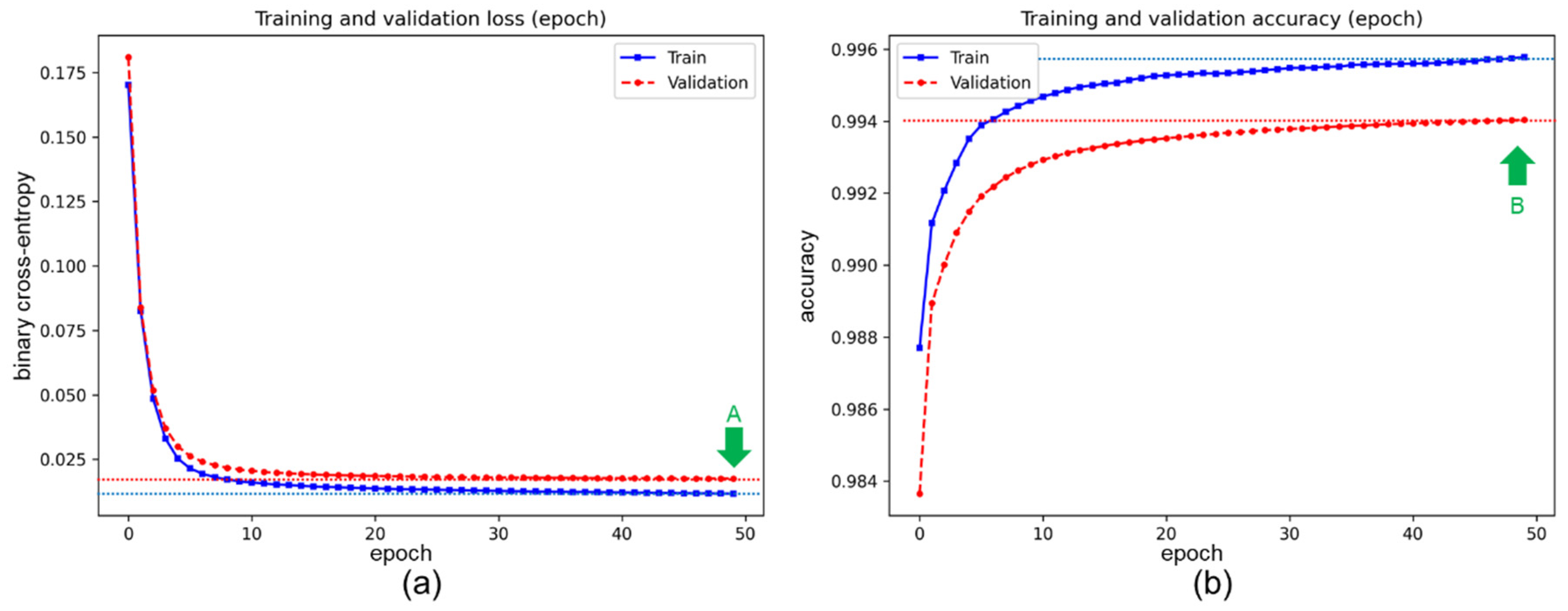
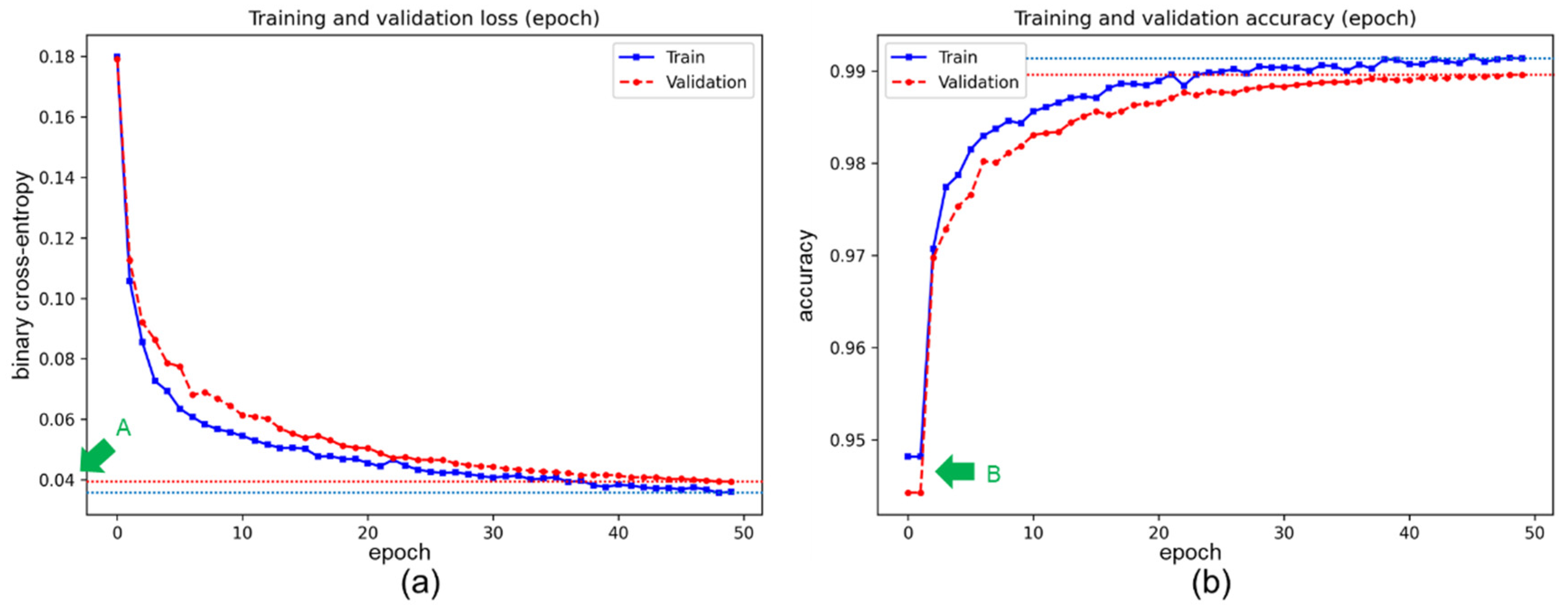
| Epoch | 50 epochs | Batch size | 5 sample per batch |
| Learning rate | 0.00005 | Optimizer | Adam |
| Loss function | Binary cross-entropy | Training set ratio | 80% of the synthetic dataset |
| Validation set ratio | 10% of the synthetic dataset | Testing set ratio | 10% of the synthetic dataset |
| Evaluation metrics | Accuracy, intersection over union (IoU), Dice score, root mean squared error (RMSE), and receiver operating characteristic curve (ROC) | ||
| Hyperparameter | Setting | Hyperparameter | Setting |
|---|---|---|---|
| Epoch | 50 epochs | Batch size | 5 sample per batch |
| Learning rate | 0.00005 | Optimizer | Adam |
| Loss function | Binary cross-entropy | Training set ratio | 80% of the synthetic dataset |
| Validation set ratio | 10% of the synthetic dataset | Testing set ratio | 10% of the synthetic dataset |
| Evaluation metrics | Accuracy, intersection over union (IoU), Dice score, root mean squared error (RMSE), and receiver operating characteristic curve (ROC) | ||
| Network | Loss | Accuracy | IoU | RMSE | ||||||||
|---|---|---|---|---|---|---|---|---|---|---|---|---|
| Train | Valid | Test | Train | Valid | Test | Train | Valid | Test | Train | Valid | Test | |
| U-Net | 0.0360 | 0.0393 | 0.0397 | 99.13% | 98.96% | 98.95% | 0.8446 | 0.8248 | 0.8255 | 0.1027 | 0.1039 | 0.1043 |
| U-Net++ | 0.0121 | 0.0211 | 0.0209 | 99.56% | 99.28% | 99.28% | 0.9182 | 0.8769 | 0.8783 | 0.0668 | 0.0744 | 0.0743 |
| NI-U-Net | 0.0102 | 0.0281 | 0.0280 | 99.63% | 99.25% | 99.24% | 0.9313 | 0.8715 | 0.8720 | 0.0665 | 0.0775 | 0.0776 |
| Furlan2019 | 0.0273 | 0.0307 | 0.0308 | 99.04% | 98.86% | 98.86% | 0.9125 | 0.9005 | 0.9001 | 0.0912 | 0.0924 | 0.0926 |
| Chiodini2020 | 0.0108 | 0.1724 | 0.1692 | 99.38% | 97.98% | 98.00% | 0.9423 | 0.8299 | 0.8330 | 0.1298 | 0.1336 | 0.1328 |
| NI-U-Net++ | 0.0117 | 0.0175 | 0.0173 | 99.58% | 99.40% | 99.41% | 0.9209 | 0.8972 | 0.8991 | 0.0665 | 0.0775 | 0.0775 |
| Loss | Accuracy | IOU | Dice | RMSE | ||||||||||
|---|---|---|---|---|---|---|---|---|---|---|---|---|---|---|
| Train | Valid | Test | Train | Valid | Test | Train | Valid | Test | Train | Valid | Test | Train | Valid | Test |
| 0.0061 | 0.0183 | 0.0151 | 99.74% | 99.54% | 99.58% | 0.8841 | 0.7223 | 0.7476 | 0.9384 | 0.8387 | 0.8556 | 0.0499 | 0.0594 | 0.0557 |
Publisher’s Note: MDPI stays neutral with regard to jurisdictional claims in published maps and institutional affiliations. |
© 2021 by the authors. Licensee MDPI, Basel, Switzerland. This article is an open access article distributed under the terms and conditions of the Creative Commons Attribution (CC BY) license (https://creativecommons.org/licenses/by/4.0/).
Share and Cite
Kuang, B.; Wisniewski, M.; Rana, Z.A.; Zhao, Y. Rock Segmentation in the Navigation Vision of the Planetary Rovers. Mathematics 2021, 9, 3048. https://doi.org/10.3390/math9233048
Kuang B, Wisniewski M, Rana ZA, Zhao Y. Rock Segmentation in the Navigation Vision of the Planetary Rovers. Mathematics. 2021; 9(23):3048. https://doi.org/10.3390/math9233048
Chicago/Turabian StyleKuang, Boyu, Mariusz Wisniewski, Zeeshan A. Rana, and Yifan Zhao. 2021. "Rock Segmentation in the Navigation Vision of the Planetary Rovers" Mathematics 9, no. 23: 3048. https://doi.org/10.3390/math9233048
APA StyleKuang, B., Wisniewski, M., Rana, Z. A., & Zhao, Y. (2021). Rock Segmentation in the Navigation Vision of the Planetary Rovers. Mathematics, 9(23), 3048. https://doi.org/10.3390/math9233048