Abstract
In this paper, we use the ARA transform to solve families of fractional differential equations. New formulas about the ARA transform are presented and implemented in solving some applications. New results related to the ARA integral transform of the Riemann-Liouville fractional integral and the Caputo fractional derivative are obtained and the last one is implemented to create series solutions for the target equations. The procedure proposed in this article is mainly based on some theorems of particular solutions and the expansion coefficients of binomial series. In order to achieve the accuracy and simplicity of the new method, some numerical examples are considered and solved. We obtain the solutions of some families of fractional differential equations in a series form and we show how these solutions lead to some important results that include generalizations of some classical methods.
1. Introduction
Fractional calculus is a field of mathematics that studies the theory and applications of integral and derivatives of a non-integer order. It becomes a vibrant area for mathematicians and scientists in their research because of its popularity and importance in modeling and describing many phenomena in many areas including quantum mechanics, plasma physics, electromagnetic theory and other different areas of science; see the books of Podlubny [1], Miller and Ross [2] and Oldham [3] and the papers by Friedrich [4], Chen and Moore [5] and Ahmad and Sivasundaram [6].
During the last decade, researchers have been interested in establishing and refining new methods to solve fractional differential equations such as the Adomian decomposition method [7], the iteration method [8,9], residual power series [10], the finite-difference method [11,12], the Laplace transform method [12,13,14,15] and the Homotopy analysis method [16]. Some of these methods give the solution in a series form which converges to the exact solution and other methods reduce the given equation into a simple one or system of equations [17,18,19,20].
In order to produce this paper, we deal with the ARA transform [21], which is a general form of the Laplace transform. In addition, the ARA transform is applicable for some functions which can’t be defined in the case of Laplace transform.
Some important theorems related to the Laplace transform have been generalized and constructed to the ARA transform.
New general formulas are established throughout applying the ARA transform on both Riemann-Liouville fractional integral and Caputo fractional derivative. The last one is implemented to solve and construct series solutions of some families of fractional differential equations.
The article is organized as follows. In Section 2, we introduce some basic definitions of fractional calculus and the ARA transform. Some properties of the ARA transform that are needed in our work also are illustrated in Section 2. In Section 3, the ARA transform is implemented to obtain new formulas by applying the ARA transform on the Riemann-Liouville fractional integral and the Caputo fractional derivative.
In Section 4, solutions of some families of fractional differential equations are introduced and discussed with some applications.
2. Definitions and Properties
In this section, we present some basic definitions and properties of fractional calculus theory and the ARA transform that are needed to construct the new formulas about the ARA solution of the fractional differential equations.
Definition 1
[1]. The Riemann-Liouville fractional integral of order of the function is defined by:
Definition 2
[1]. The Caputo fractional derivative of order of the function is defined by:
Recently, Saadeh et al. [21] introduced a new integral transform, called the ARA transform, which is applied to solve ordinary and partial differential equations.
Definition 3
[21]. The ARA transform of order n of the continuous function , is defined by:
Definition 4.
The binomial formula is written as:
where
Definition 5.
The Mittag-Leffler function (cf. [22,23]) is defined by:
In the following we introduce some basic properties of the ARA transform [21] that are essential in our research.
Property 1.
(Existence of the ARA Transform)
Ifis a piecewise continuous function on every finite intervaland satisfies:
then the ARA transform exists for all.
Property 2.
(Linearity Property)
Let and be two functions in which the ARA transform exists. Then
where α and β are nonzero constants.
Property 3.
(Shifting in n—Domain)
Property 4.
(The ARA Transform for Derivatives)
Property 5.
(Convolution)
Property 6.
The ARA transform ofis given by:
In the following arguments, we introduce the dualities between the ARA transform and some well-known transforms.
- Duality to Laplace transform [24]and
- Duality to Sumudu transform [25]Putting , we get
- Duality to Shehu transform [26]Putting = 1, we getand
3. The ARA Transform of Fractional Operators
In this section we present two basic theorems about the application of ARA transform on the Riemann-Liouville fractional integral and the Caputo fractional derivative and construct new formulas to solve the target equations.
Theorem 1.
The ARA transform of the Riemann-Liouville fractional integral of order α > 0 of the function g(t) is given by:
whereis the binomial coefficient.
Proof of Theorem 1.
The Riemann-Liouville fractional integral of the function g(t) can be written as
Applying the ARA transform on both sides of Equation (1), to get
Using Property 5, we have
□
Theorem 2.
The ARA transform of the Caputo fractional derivative of order α > 0 of the function g(t) is given by:
for m − 1 < α ≤ m.
Proof of Theorem 2.
Applying the ARA transform on the Caputo fractional derivative of the function g(t), we have:
Changing the order of integration, we get
Letting in Equation (2) leads to
Using the binomial formula, Equation (3) can be written as
Thus,
From the definition of the ARA transform of order one , we obtain
Property 6 and the definition of the ARA transform yield
This completes the proof. □
Remark 1.
(Special Cases of Theorem 2)
4. Solutions of Families of Fractional Differential Equations
Throughout this section, we derive three basic theorems to construct series solutions of fractional differential equations of the first and second order. Mathematica software is used to compute and simplify the results.
Theorem 3.
The solution of the fractional differential equation
where is a piecewise continuous function in every finite intervalin which the ARA transform exists, with initial conditions
is given by
Proof of Theorem 3.
Applying the ARA transform of second order on both sides of Equation (6), we get:
Using Equation (5) with m = 2,
Using Property 4 with n = 2 for m = 1 and m = 0 respectively, and the initial conditions in (7)
Again, using Property 4 with n = 1 and m = 2, and the initial conditions in (7)
After simple computations, Equation (8) becomes
Solving the ordinary differential Equation (9), we get:
Now expand the term in the following form
Thus, Equation (10) can be written as
Applying the inverse ARA transform of order 1 on Equation (11), we have
□
Example 1.
The fractional differential equation
with initial conditions g(0) = 1 and g′(0) = 0, has the following solution
Putting α = 0 in Theorem 3 we get the following results.
Corollary 1.
The solution of the fractional differential equation
wherewith the initial conditionsandis
Example 2.
The fractional differential equation
with initial conditionsand, has the following solution
The exact solution of Equation (12) can be obtained at α = 2 as the following
Table 1 shows the absolute error between the exact solution (14) and the solution obtained in Equation (13) with α = 2.

Table 1.
The absolute error at α = 2 for Example 2.
Figure 1 illustrates the solution behavior of the fractional differential Equation (12) at various values of α. Blue line: exact solution at α = 2, dashed line at α = 1.9, dotted line at α = 1.8, dash. dotted line at α = 1.6, large dash line at α = 1.5.
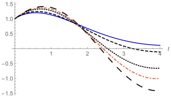
Figure 1.
The solution behavior of Equation (12).
Corollary 2.
The solution of the harmonic vibration equation [27]
with the initial conditions and is given by
Theorem 4.
The solution of the fractional differential equation
where is a piecewise continuous function in every finite intervalin which the ARA transform exists, with initial conditions
is given by
Proof of Theorem 4.
Applying the ARA integral transform of second order on both sides of Equation (15), we get
Using Equation (5) with m = 2,
Using Property 4 with n = 2 for m = 2 and m = 0 respectively, and the initial conditions in (16), we get
Again, using Property 4 with n = 1 and m = 2, and the initial conditions in (16),
After simple computations, Equation (17) can be written as
Solving the ordinary differential Equation (18), we get
Now, to get our target, we expand the term as follows
Thus, Equation (19) can be written as
Applying the inverse ARA transform on Equation (20), we have
□
Example 3.
The fractional differential equation
with initial conditionsandhas the following series solution
Putting in Theorem 2 we get the following result.
Corollary 3.
The solution of the fractional differential equation of the form:
where, with initial conditionsandis
Theorem 5.
The solution of the fractional differential equation of the form
where is a piecewise continuous function in every finite intervalin which the ARA transform exists, with initial condition
is:
Proof of Theorem 5.
Applying the ARA transform of the second order on both sides of Equation (21) we get
Using Equation (5) of Remark 1 with and the initial condition (22)
Again, using Equation (4) with and we have
Solving the ordinary differential Equation (23), we get
To get our result we apply the inverse ARA transform of order 1, of both sides of Equation (24).
□
5. Conclusions
In this work a new technique has been developed for solving families of fractional differential equations. We introduced new formulas using the ARA transform to achieve series solutions of differential equations with fractional order. A formula of the ARA transform for Caputo fractional derivative was established and implemented to solve examples and obtain new results. Three main theorems are presented, including the series solution of some fractional differential equations of first and second orders. In future work, we intend to solve partial differential equations and fractional integral equations using new formulas combined with the ARA transform.
Author Contributions
Data curation, A.Q., R.S. and A.B.; formal analysis, R.S., A.Q. and A.B.; investigation, A.B., R.S. and A.Q.; methodology, R.S., A.B. and A.Q.; project administration, A.Q., R.S. and A.B.; resources, A.B., R.S. and A.Q.; writing—original draft, A.Q., R.S. and A.B.; writing—review and editing, A.Q., R.S. and A.B. All authors have read and agreed to the published version of the manuscript.
Funding
This research is funded by the Deanship of Research in Zarqa University, Jordan.
Data Availability Statement
Not applicable.
Acknowledgments
The authors express their gratitude to the dear unknown referees and the editor for their helpful suggestions, which improved the final version of this paper.
Conflicts of Interest
The authors declare no conflict of interest.
References
- Podlubny, I. Fractional Differential Equations; Academic Press: San Diego, CA, USA, 1999; ISBN 0-1255-8840-2. [Google Scholar]
- Miller, K.S.; Ross, B. An Introduction to the Fractional Calculus and Fractional Differential Equations; John Wiley: New York, NY, USA, 1993; ISBN 0-4715-8884-9. [Google Scholar]
- Oldham, K.B.; Spanier, J. The Fractional Calculus; Academic Press: New York, NY, USA; London, UK, 1974. [Google Scholar]
- Friedrich, C. Relaxation and retardation functions of the Max well model with fractional derivatives. Rheol. Acta 1991, 30, 151–158. [Google Scholar] [CrossRef]
- Chen, Y.Q.; Moore, K.L. Analytical stability bounded for a class of delayed fractional-order dynamic systems. Nonlinear Dyn. 2002, 29, 191–200. [Google Scholar] [CrossRef]
- Ahmad, B.; Sivasundaram, S. Existence results for nonlinear impulsive hybrid boundary value problems involving fractional differential equations. Nonlinear Anal. Hybrid Syst. 2009, 3, 251–258. [Google Scholar] [CrossRef]
- Adomian, A. A review of the decomposition method and some recent results for nonlinear equations. Comput. Math. Appl. 1990, 21, 101–127. [Google Scholar] [CrossRef] [Green Version]
- Inc, M. The approximate and exact solutions of the space- and time-fractional Burgers equations with initial conditions by variational iteration method. J. Math. Anal. Appl. 2008, 345, 476–484. [Google Scholar] [CrossRef] [Green Version]
- Odibat, Z.; Momani, S. Application of variational iteration method to nonlinear differential equations of fractional order. Int. J. Nonlinear Sci. Numer. Simul. 2006, 7, 27–34. [Google Scholar] [CrossRef]
- Saadeh, R.; Alaroud, M.; Al-Smadi, M.; Ahmad, R.; Din, U. Application of Fractional Residual Power Series Algorithm to Solve Newell–Whitehead–Segel Equation of Fractional Order. Symmetry 2019, 11, 1431. [Google Scholar] [CrossRef] [Green Version]
- Edwan, R.; Saadeh, R.; Hadid, S.; Al-Smadi, M.; Momani, S. Solving Time-Space-Fractional Cauchy Problem with Constant Coefficients by Finite-Difference Method. In Computational Mathematics and Applications, Springer Proceedings in Mathematics; Zeidan, D., Padhi, S., Burqan, A., Ueberholz, P., Eds.; Springer: Singapore, 2020; Volume 1, pp. 25–46. [Google Scholar]
- Saadeh, R. Numerical solutions of fractional convection-diffusion equation using finite-difference and finite-volume schemes. J. Math. Comput. Sci. 2021, 11, 7872. [Google Scholar]
- Carpinteri, A.; Mainardi, F. Fractals and Fractional Calculus in Continuum Mechanics; Springer: New York, NY, USA, 1997. [Google Scholar]
- Kazem, S. Exact solution of some linear fractional differential equations by Laplace transform. Int. J. Nonlinear Sci. 2013, 16, 3–11. [Google Scholar]
- Burqan, A.; El-Ajou, A.; Saadeh, R.; Al-Smadi, A. New efficient technique using Laplace transforms and smooth expansions to construct a series solution to the time-fractional Navier-Stokes equations. Alex. Eng. J. 2021. [Google Scholar] [CrossRef]
- Das, S.; Gupta, P. Homotopy analysis method for solving fractional diffusion equation. Int. J. Comput. Math. 2011, 88, 578–588. [Google Scholar] [CrossRef]
- Maitama, S.; Zhao, W. Homotopy analysis Shehu transform method for solving fuzzy differential equations of fractional and integer order derivatives. Comput. Appl. Math. 2021, 40, 1–30. [Google Scholar] [CrossRef]
- Maitama, S.; Zhao, W. Homotopy perturbation Shehu transform method for solving fractional models arising in applied sciences. J. Appl. Math. Comput. Mech. 2021, 20, 71–82. [Google Scholar] [CrossRef]
- Qazza, A.; Hatamleh, R.; Alodat, N. About the Solution Stability of Volterra Integral Equation with Random Kernel. Far East J. Math. Sci. 2016, 100, 671–680. [Google Scholar] [CrossRef]
- Qazza, A.; Hatamleh, R. The existence of a solution for semi-linear abstract differential equations with infinite B chains of the characteristic sheaf. Int. J. Appl. Math. 2018, 31, 611–620. [Google Scholar] [CrossRef]
- Saadeh, R.; Qazza, A.; Burqan, A. A new integral transform: ARA transform and its properties and applications. Symmetry 2020, 12, 925. [Google Scholar] [CrossRef]
- Mittag-Leffleri, G. Sur La Nouvelle Fonction Ea(x); Comptes Rendus de l’Académie des Sciences: Paris, France, 1903. [Google Scholar]
- Tomovski, Z.; Hilfer, R.; Srivastava, H.M. Fractional and operational calculus with generalized fractional derivative operators and Mittag-Leffler type functions. Integral Transform. Spec. Funct. 2011, 21, 797–814. [Google Scholar] [CrossRef]
- Widder, D.V. The Laplace Transform; Princeton University Press: London, UK, 1946. [Google Scholar]
- Watugula, G.K. Sumudu transform: A new integral transform to solve differential equations and control engineering problems. Int. J. Math. Edu. Sci. Technol. 1993, 24, 35–43. [Google Scholar] [CrossRef]
- Maitama, S.; Zhao, W. New integral transform: Shehu transform a generalization of Sumudu and Laplace transform for solving differential equations. Int. J. Anal. Appl. 2019, 17, 167–190. [Google Scholar]
- Gorenflo, R.; Mainardi, F.; Srivastava, H.M. Special functions in fractional relaxation-oscillation and fractional diffusion-wave phenomena. In Proceedings of the Eighth International Colloquium on Differential Equations, Plovdiv, Bulgaria, 18–23 August 1997. [Google Scholar]
Publisher’s Note: MDPI stays neutral with regard to jurisdictional claims in published maps and institutional affiliations. |
© 2021 by the authors. Licensee MDPI, Basel, Switzerland. This article is an open access article distributed under the terms and conditions of the Creative Commons Attribution (CC BY) license (https://creativecommons.org/licenses/by/4.0/).