Deterministic Chaos Detection and Simplicial Local Predictions Applied to Strawberry Production Time Series

Abstract

In this work, we attempted to find a non-linear dependency in the time series of strawberry production in Huelva (Spain) using a procedure based on metric tests measuring chaos. This study aims to develop a novel method for yield prediction. To do this, we study the system’s sensitivity to initial conditions (exponential growth of the errors) using the maximal Lyapunov exponent. To check the soundness of its computation on non-stationary and not excessively long time series, we employed the method of over-embedding, apart from repeating the computation with parts of the transformed time series. We determine the existence of deterministic chaos, and we conclude that non-linear techniques from chaos theory are better suited to describe the data than linear techniques such as the ARIMA (autoregressive integrated moving average) or SARIMA (seasonal autoregressive moving average) models. We proceed to predict short-term strawberry production using Lorenz’s Analog Method.

1. Introduction

The strawberry of Huelva (strawberry from Spain) belongs to the select group of agricultural activities in which Spain is the absolute leader in the European Union [1]. Huelva accounts for 9% of world strawberry production and 25% of that of the European Union; it is the second-largest area of production, technology, and research in the world in this sector behind California [2] and contributes more than 400 million euros to the province in direct total agricultural production value [3].

On the other hand, the evolution of strawberry production is sensitive to price fluctuations [4,5]. Strawberry is a free-market crop with no entry or exit barriers, without intervention prices or production controls. The price of strawberries is determined strictly by the free interaction of supply and demand. Knowing the future productions of these time series could mean a considerable increase in profitability for the strawberry-producing sector [1], since a large distribution usually results in sales programs with heavy penalties for non-compliance.

Yield forecast approaches are basically divided into single-factor time series models and multi-factor models. The former considers time as an independent variable and builds up mathematical models based on the yield time series to produce future predictions; the latter also considers the main influential factors in the system under study. As a first approach to the study of strawberry yield predictions, we considered only single-factor models. Multi-factor models are generally more time consuming and require extensive user intervention. In addition, external factors such as prices, costs, crop characteristics, consumer behavior, or climatic conditions often require data that may be unavailable or difficult to obtain. Finally, to use the forecasting model in the future, predictions for such factors are also required, the quality of which will depend on the accuracy of the forecasts. Thus, it is worth considering whether single-factor models provide acceptable forecasts.

Typically, autoregressive integrated moving average (ARIMA) or seasonal autoregressive moving average (SARIMA) models have been widely used in recent years for modeling and to make predictions in the livestock [6,7] and agricultural [8,9,10] sectors. In this article, we discuss an alternative non-linear method for the cases in which the resulting series is not stationary. Although we find many emerging non-linear techniques that can be used to make both short-term and long-term predictions on non-stationary chaotic data, such as the sparse identification of nonlinear dynamics (SINDy) algorithm [11] widely used to model non-linear dynamic systems and make predictions on them [12,13,14,15], or non-linear systems reconstruction techniques that allow the regeneration of time series subjected to white noise, which would allow a new study of stationarity and eliminate the disturbances associated with the observed variable [16,17], in this work, we focus on maximal Lyapunov exponents.

Deterministic chaos theory has made possible the modeling and forecasting of many time series traditionally considered as the noise of purely random behavior. There are many fields in which the deterministic chaos methodology is being applied successfully, from the climate [18] to COVID-19 [19]. For this reason, the construction and analysis of chaotic predictive models are of special interest. However, the empirical detection of chaotic dynamics is an extremely subtle problem because the strange attractor’s reconstruction that originates the deterministic dynamics is sensitive to the parameters used in non-linear tests [20].

This study focuses on this sector and proposes a novel method for yield prediction in relation to the recent literature on time series predictive models. First, we detected deterministic chaos by computing the maximum Lyapunov exponents of the time-series and observing that they are positive. Secondly, since these cannot be generated by linear models such as ARIMA [21] or SARIMA [22], we used the analog method [23,24,25]—a non-linear forecasting technique consisting of analyzing, for each of the final observations of the series, the possibilities of short-term forecasting. We intended to study whether the reconstructed phase space’s points behave according to the principle of prediction by analogous occurrences; that is, we try to see if nearby points evolve in the short-term with similar trajectories within the phase space.

Since the description of the method of analogs by Lorenz [26], this method has gained popularity for forecasting and has been applied in many studies [27,28,29,30], offering even more accurate results than other approaches that apply machine learning techniques [31,32].

The paper is organized as follows: in Section 2.1, the time series are described; Section 2.2 analyzes stationarity; in Section 2.3, the spectral analysis is performed; in Section 2.4, the maximum Lyapunov exponents are computed; in Section 3, analogous occurrences are used to obtain the predictions; in Section 4, our conclusions are discussed and presented.

2. Materials and Methods

This research uses R and Haskell programming languages, which are applied for time series forecasting.

2.1. Description of the Data

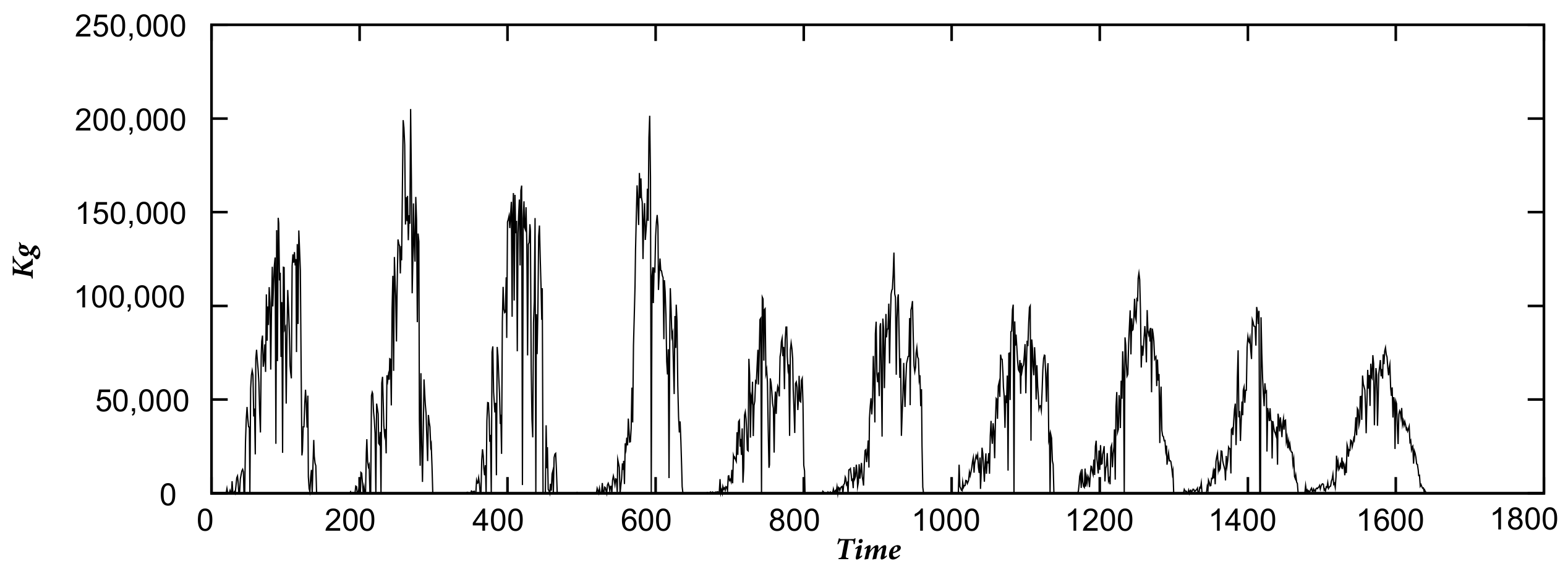
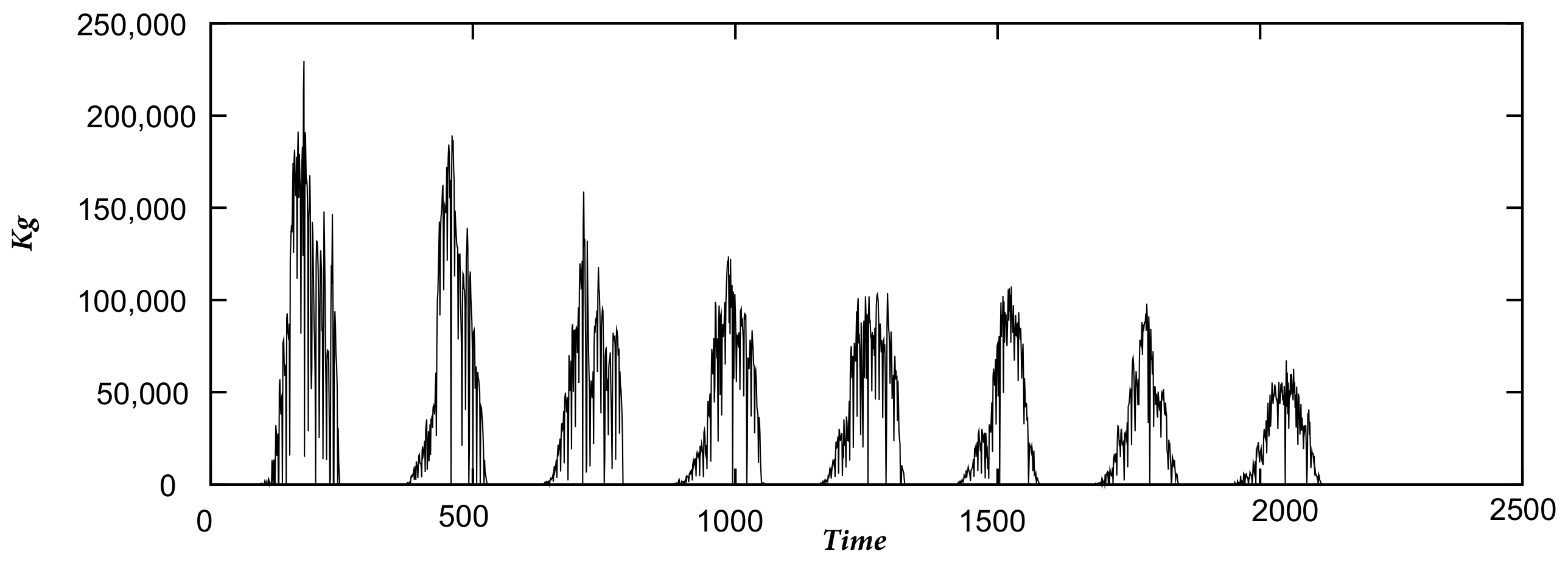
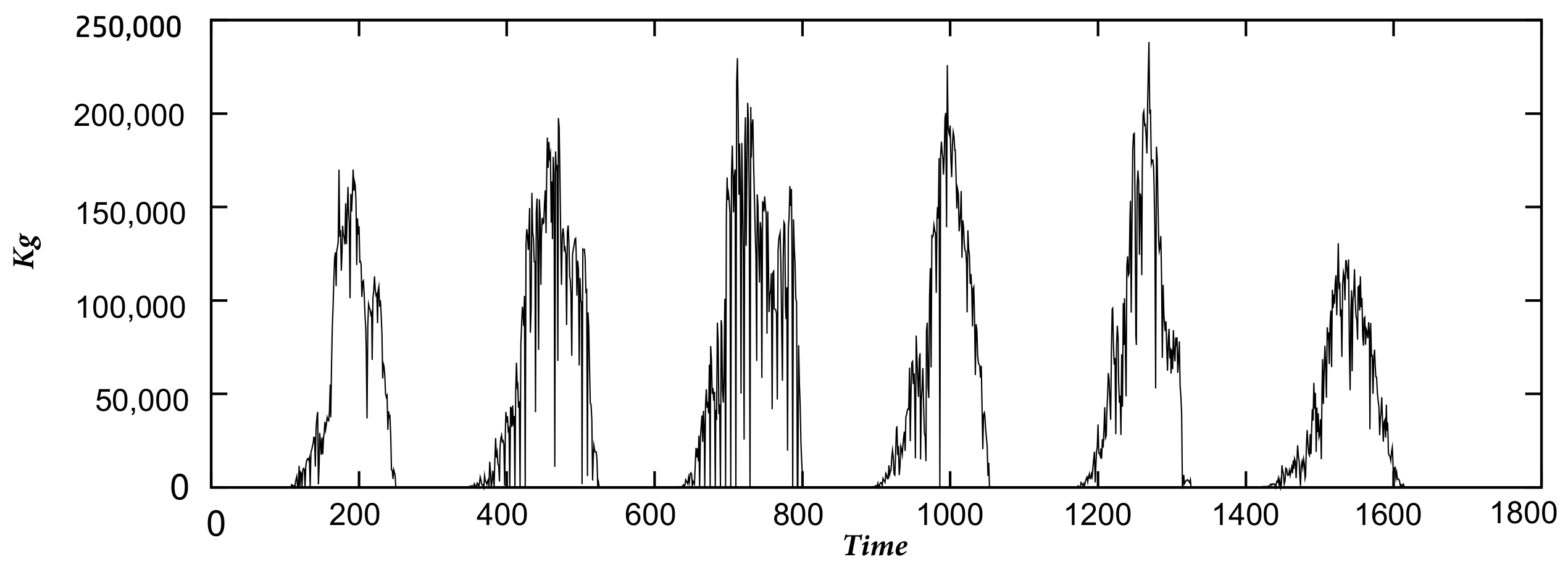
We work with time series of the daily production of three large agri-food cooperatives in the province of Huelva (coop1, coop2, and coop3) during a time interval ranging from 6 to 10 years. The time-series data refer to the total weight of strawberries, in kilograms, picked in one day. The coop1 data were collected over 10 strawberry picking seasons, from January 2011 to June 2020. The coop2 data cover 8 seasons, from January 2013 to June 2020. Finally, the coop3 data cover 6 periods, from January 2015 to June 2020.

Since the fruit picking season begins on a different date each year, we handled the datasets as follows: if for each company, $d_1$ corresponds to the first day of the period that started earlier and $d_2$ to the last day of the period that ended later, then we establish that each period starts at $d_1$ and ends at $d_2$, filling in the days where there is no fruit picking with zeros. Finally, we join the series of each period in chronological order, obtaining a single time series for each company. The time series of coop1 contains 1642 data points, that of coop2 2130 data points, and that of coop3 1633 data points, as represented in Figure 1, Figure 2 and Figure 3.

2.2. Stationarity

One of the characteristics that distinguish time series from other types of statistical data is that, in general, the data at different instants of time can be correlated. The most classical methodology for the analysis of time series is that of Box and Jenkins [21,33,34,35], which allows the identification and estimation of ARMA models (autoregressive and moving averages). These models assume the hypothesis that the series is stationary (or may become stationary from a simple transformation) and follow a linear model.

In this sense, and without carrying out an exhaustive analysis, as can be seen in

Table 1. Local means and standard errors of production.

Period	coop1		coop2		coop3
	Mean	Error	Mean	Error	Mean	Error
2011	42,202	3598	–	–	–	–
2012	42,830	4382	–	–	–	–
2013	46,837	4448	34,364	3321	–	–
2014	47,946	4632	49,938	4088	–	–
2015	31,378	2427	44,235	2961	35,621	3124
2016	34,875	2959	41,278	2814	47,378	3692
2017	33,340	2421	28,908	2166	53,099	4029
2018	34,422	2765	24,656	2106	44,588	3744
2019	28,095	2159	29,036	2119	43,042	3724
2020	28,791	1845	22,207	1474	30,708	2353

, for each period of the time series, the fluctuation of the sample means is greater than the standard error, which shows that the series is not stationary.

It was also not possible to obtain a stationary time series by taking differences or logarithms or using seasonal autoregressive moving average (SARIMA) [36,37,38,39,40] as the sources that manage daily data use a short seasonal component; that is, the seasonal component is not very far from the data to be predicted, unlike in our work, where the seasonal component has a lag of 317 days, which makes its use computationally very expensive.

2.3. Fourier Analysis

To differentiate between random, stochastic, or chaotic non-linear deterministic processes, we used the Fourier transform to compute the time series’ power spectra. Thus, a series with very irregular temporal variability will have a smooth and continuous spectrum, indicating that all frequencies in a certain range or band of frequencies are excited by this process. On the contrary, a purely periodic or quasi-periodic process, or a superposition of them, is described by a single “line” or a finite number of “lines” in the frequency domain. Between these two extremes, chaotic non-linear deterministic processes can have peaks superimposed on a continuous and highly rippled background.

The Fourier transform [21,41,42,43,44,45,46], which is a standard tool for time-series analysis in both stationary and non-stationary series, provides a linear decomposition of the signal into Fourier bases (i.e., sine and cosine functions of different frequencies) and establishes a one-to-one correspondence between the signal at certain times (time domain) and how certain frequencies contribute to the signal, as well as how the phase of each oscillation is related to the phases of the other oscillations (frequency domain).

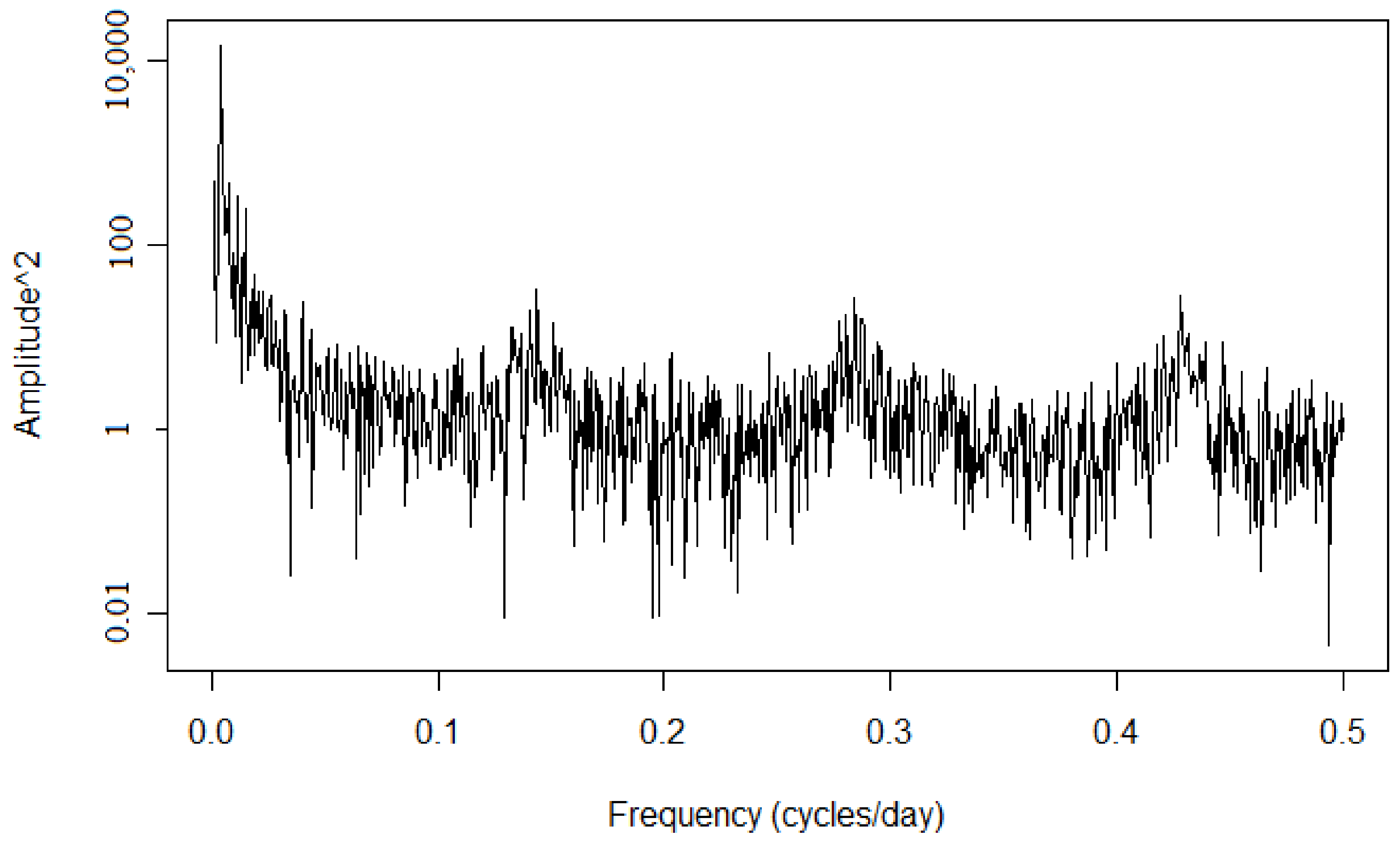
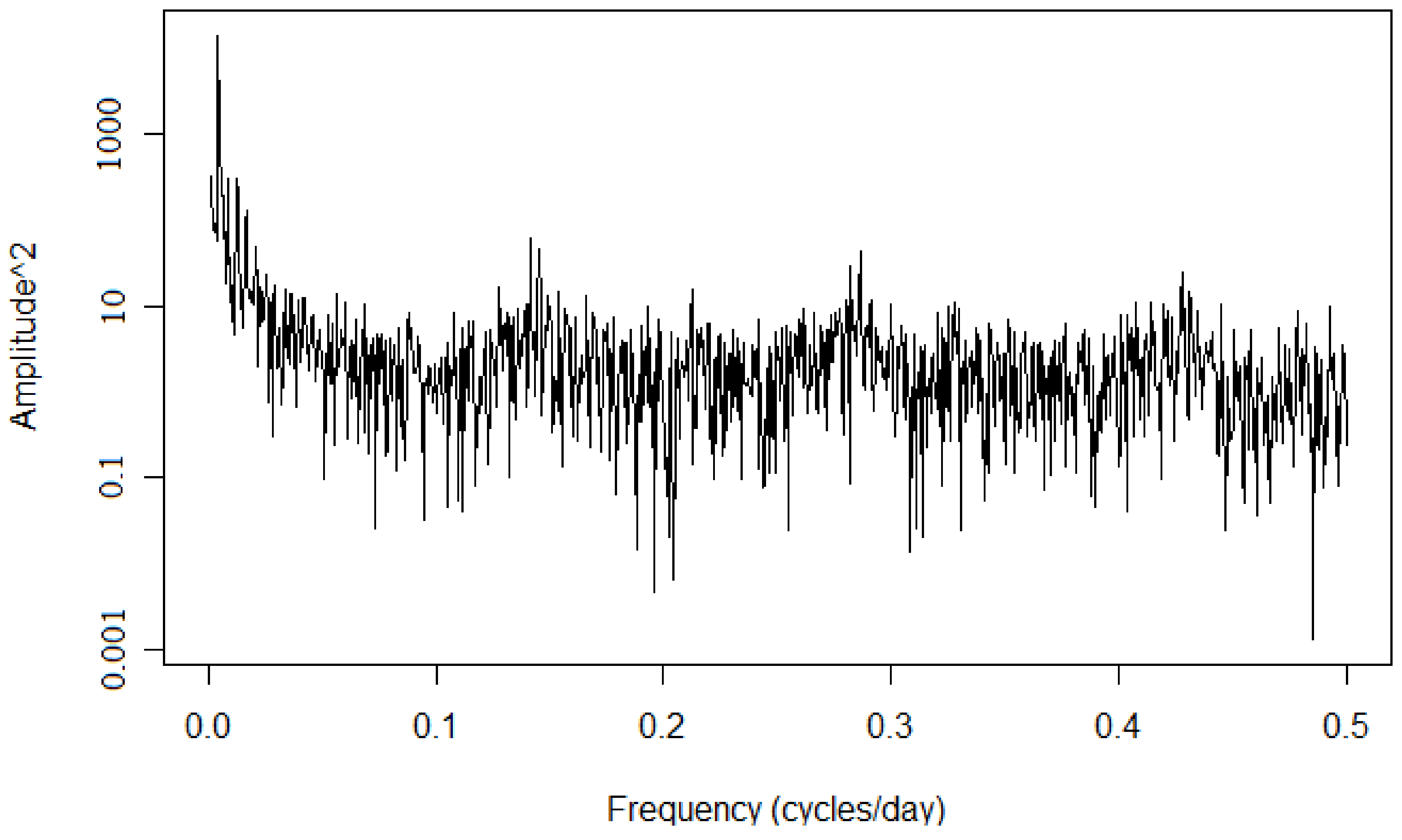
Figure 4, Figure 5 and Figure 6 show the log–log analysis of the squared amplitude against the frequency in cycles/day, presenting a broad spectrum for each company. Therefore, we can conclude that the data are neither periodic nor quasi-periodic. Furthermore, the data do not correspond to white noise. Wide peaks are observed at different frequencies, showing the influence of the past in both the short and long term, representing a seasonal influence.

2.4. Lyapunov Exponents

Now that we know that the time series studied are not stationary, periodic, quasi-periodic, or stochastic, we study the series from the point of view of nonlinear deterministic processes. This section discusses the sensitivity of these dynamic systems to initial conditions by computing the maximal Lyapunov exponent of each series [47,48].

In chaotic systems, the distance between two neighboring points in phase space diverges exponentially, and therefore, even if the system is deterministic, the prediction is only possible for a short period in the future. The exponent that characterizes this exponential divergence is the Lyapunov exponent [49,50]. In this way, only a positive exponent can show sensitivity to initial conditions, so the long-term behavior of any specified initial condition with uncertainty cannot be predicted.

Some non-linear techniques compatible with small data time series, such as the Lyapunov maximal exponent calculation, are only guaranteed to work with stationary data. This problem can be circumvented using over-embedding for sufficiently high embedding dimensions and data that depend to some extent on some (unknown) parameters, and techniques designed for stationary data can be applied [51,52,53]. Furthermore, whether the series is appropriate to compute the exponent (and other non-linear quantities) can be checked by observing how well the computation converges to the overall value when increasingly large parts of the time series are used (for example, exponents for the first and second half of the data must exist and should agree with the value computed for the whole series). Finally, when a “smooth” transformation is applied to the series (such as constructing the series of the differences), these quantities should not vary either.

Since the exact definition of the Lyapunov exponent involves limits of distances (and thus points that are arbitrarily close) and we only have a finite time series, a finite approximation must be used. Several algorithms for the computation of Lyapunov exponents of finite time series have been proposed in the literature ([48,54,55]). We use the algorithm by Rosenstein et al. [56] and by [47], which is presented below.

Given a time series $s_1,\dots ,s_k$, we use a time-delay embedding to form a series ${\mathbf{s}}_1,\dots ,{\mathbf{s}}_N$ in Euclidean m-dimensional space [51,57,58]. We choose a distance $\epsilon >0$ and define the map

$$S(\Delta n)=\frac{1}{N}\sum _{n_0=1}^{N}ln\left(\frac{1}{\left|\mathcal{U}\right({\mathbf{s}}_{n_0}\left)\right|}\sum _{{\mathbf{s}}_n\in \mathcal{U}\left({\mathbf{s}}_{n_0}\right)}\mathrm{d}({\mathbf{s}}_{n_0+\Delta n},{\mathbf{s}}_{n+\Delta n})\right)$$

where $\mathcal{U}\left({\mathbf{s}}_{n_0}\right)$ is the ball centered at ${\mathbf{s}}_{n_0}$ with radius $\epsilon$ and d is the Euclidean distance. If the graph of $S(\Delta n)$ shows a linear increase for some range of values of $\Delta n$, then there is a maximal Lyapunov exponent for ${\mathbf{s}}_1,\dots ,{\mathbf{s}}_N$, and its value is the slope of the graph. This value must be consistent for different choices of the embedding dimension and the radius $\epsilon$; that is, it should not differ for different values of $\epsilon$ provided it is small enough and for dimensions above some dimension $m_0$.

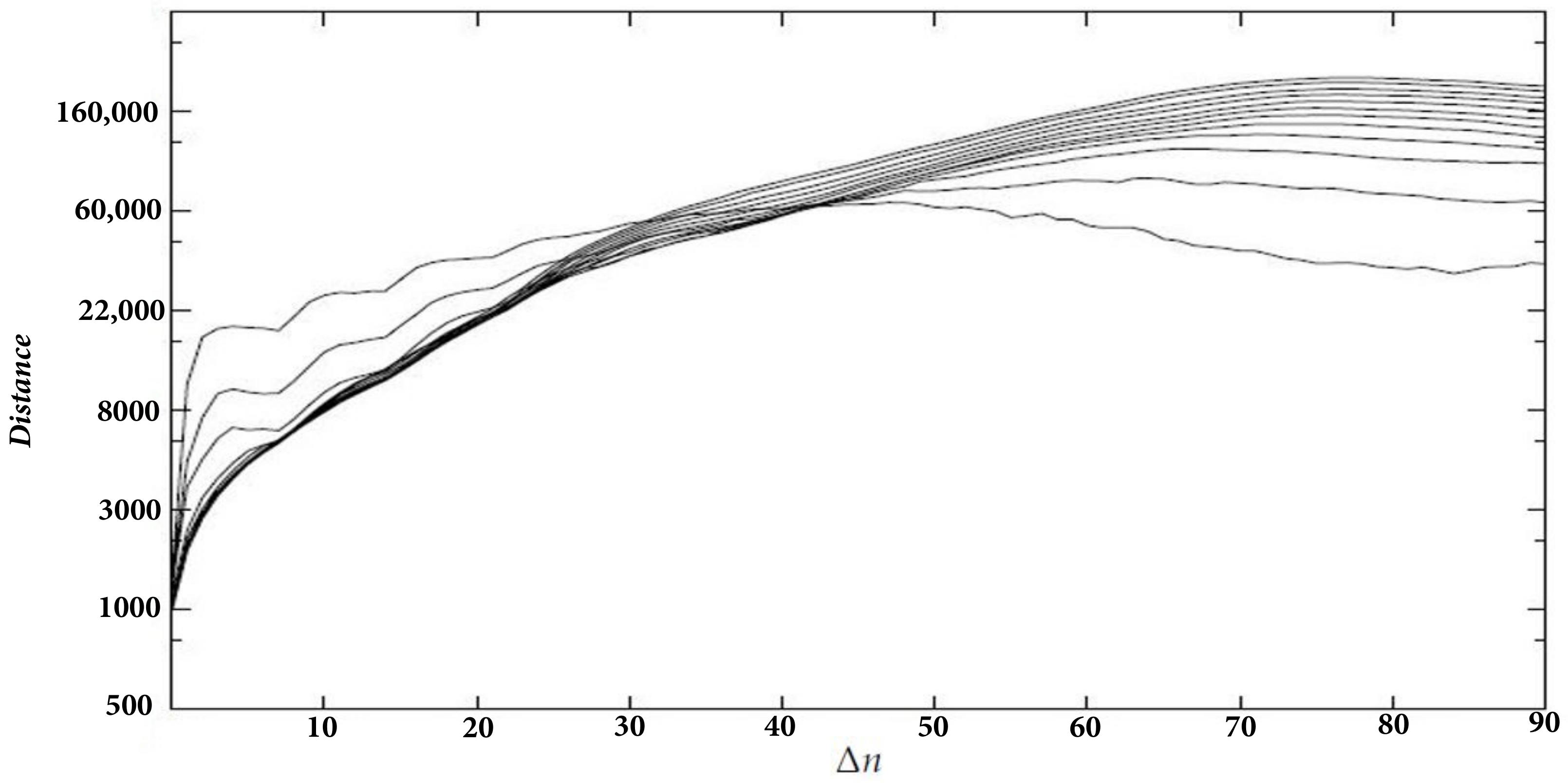
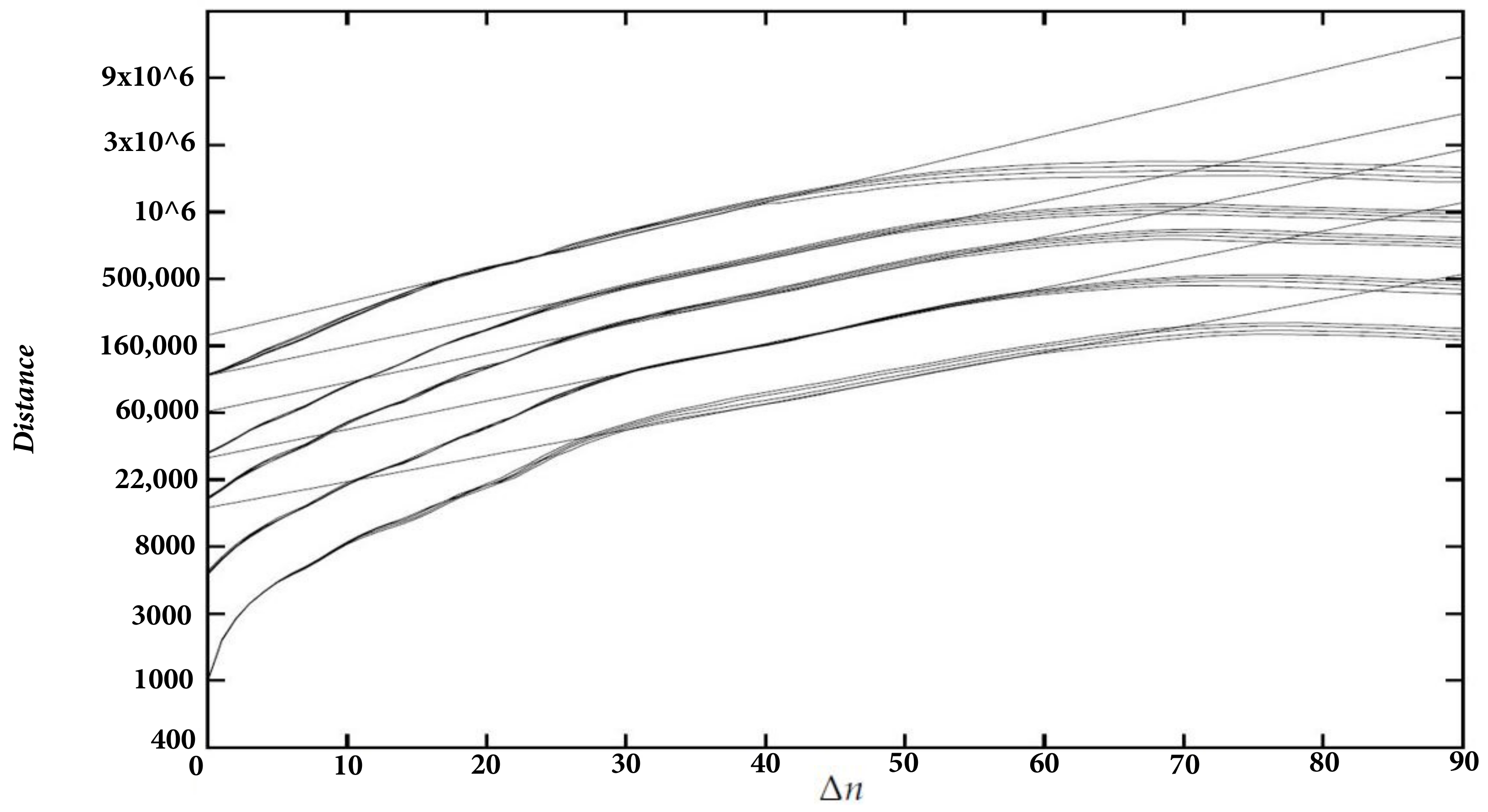
In Figure 7, we show the graphs of ${\mathrm{e}}^{S(\Delta n)}$ on a logarithmic scale (which has the same slope as $S(\Delta n)$ on a linear scale, but the values on the y axis represent distances instead of logarithms of distances) for the series of coop1, for $\Delta n$ varying between 0 and 90, with embedding dimensions 2 to 13, $\epsilon =2500$, and a delay of 1 day [59]. There is a linear increase for $\Delta n$ between 36 and 60 and dimensions 5 and above. This suggests the existence of an attractor.

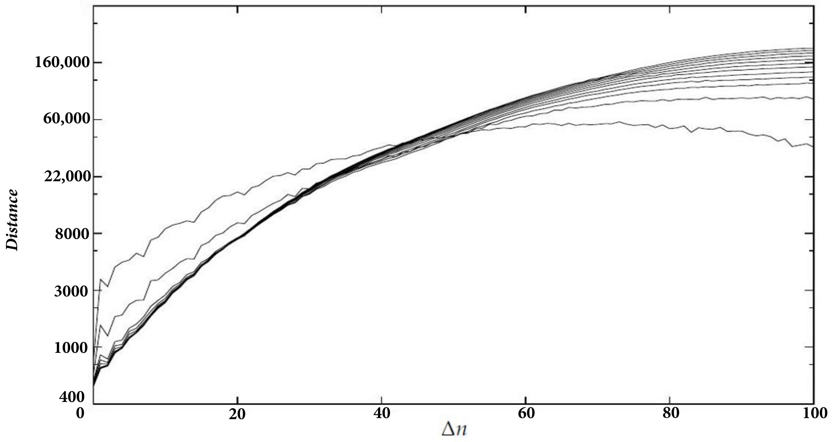
In Figure 8, we conducted the same analysis for coop2. We chose a delay of 2 days, $\epsilon$ = 2000, a $\Delta n$ ranging from 0 to 100, and a dimension ranging from 2 to 13. We observe a linear increase between 38 and 52 for dimensions 5 and above.

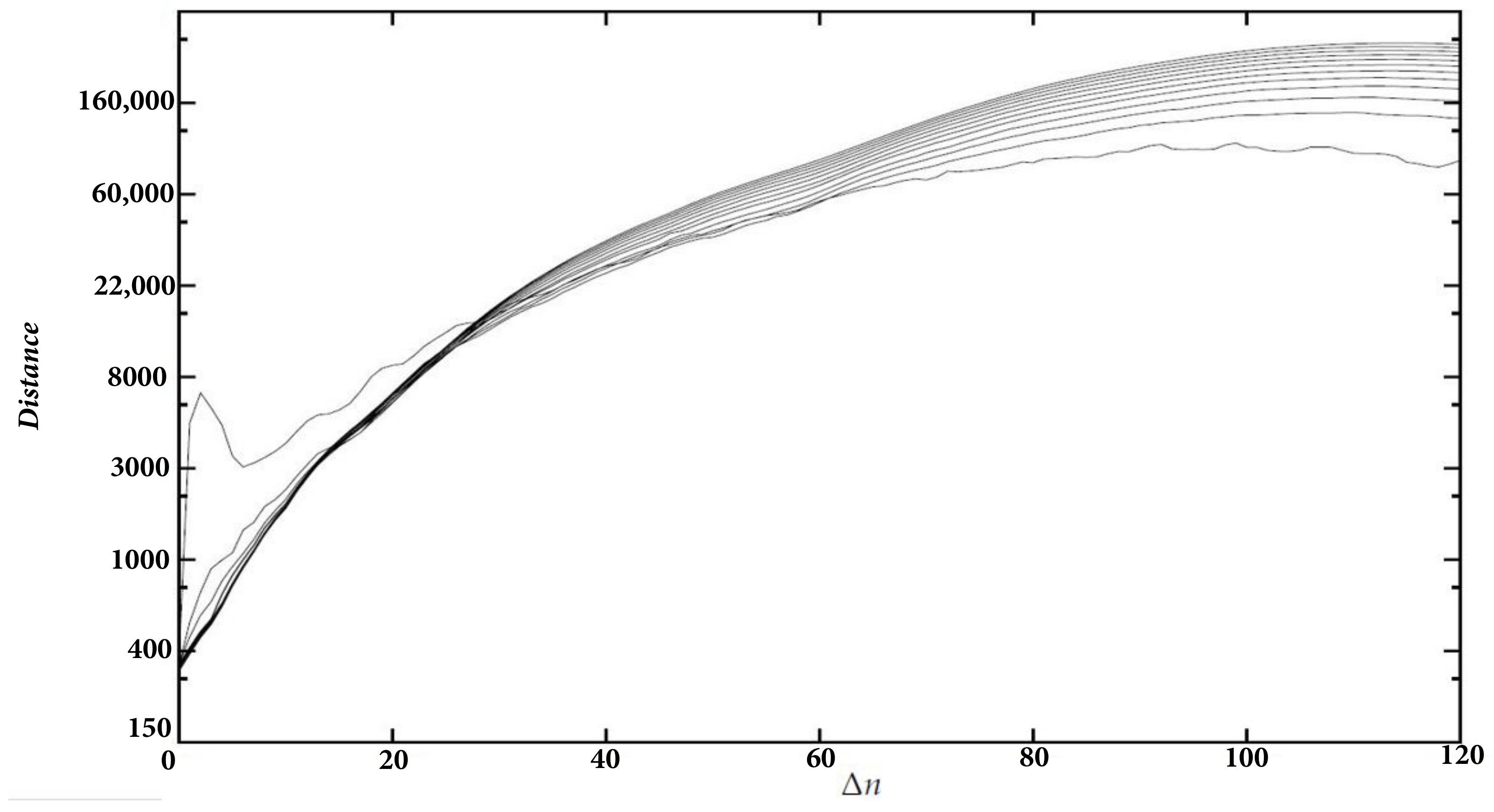
Finally, Figure 9 shows the graphs for coop3. The delay is 1 day, the dimensions range from 2 to 13, $\epsilon$ = 1000, and $\Delta n$ is between 0 and 120. There is a linear increase for dimensions above 4 and $\Delta n$ between 46 and 74.

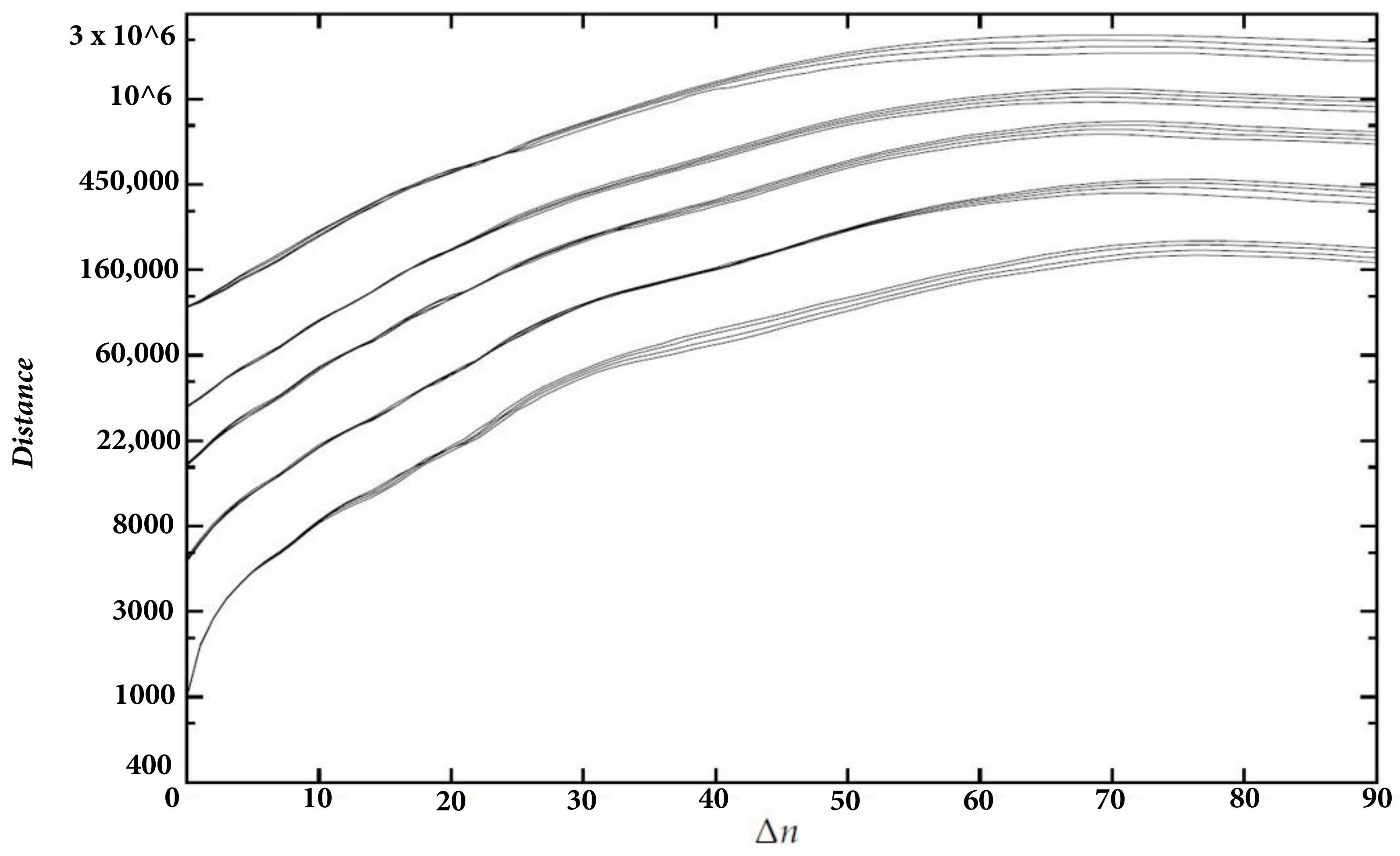
Now, we verify that there are linear increases for other values of the radius and compute the exponent. In Figure 10, we plotted the graphs of coop1 for $\epsilon =$ 2500, 5000, 7000, 9000, and 14,000 and dimensions between 10 and 13, again with a delay of 1 day. Each group of curves corresponds to a value of $\epsilon$. For the sake of visibility, we displaced each curve a given amount upwards depending on $\epsilon$.

Using the least-squares method, we fitted lines to the five curves corresponding to dimension 10 and obtained Figure 11.

Table 2. Maximal Lyapunov exponents for coop1.

$\mathit{\epsilon }$	Range $\mathbf{\Delta }\mathit{n}$	Exponent	Coefficient
2500	$[36,60]$	$0.038733$	$0.999612$
5000	$[33,50]$	$0.042351$	$0.999078$
7000	$[34,50]$	$0.043439$	$0.999411$
9000	$[32,47]$	$0.043454$	$0.999949$
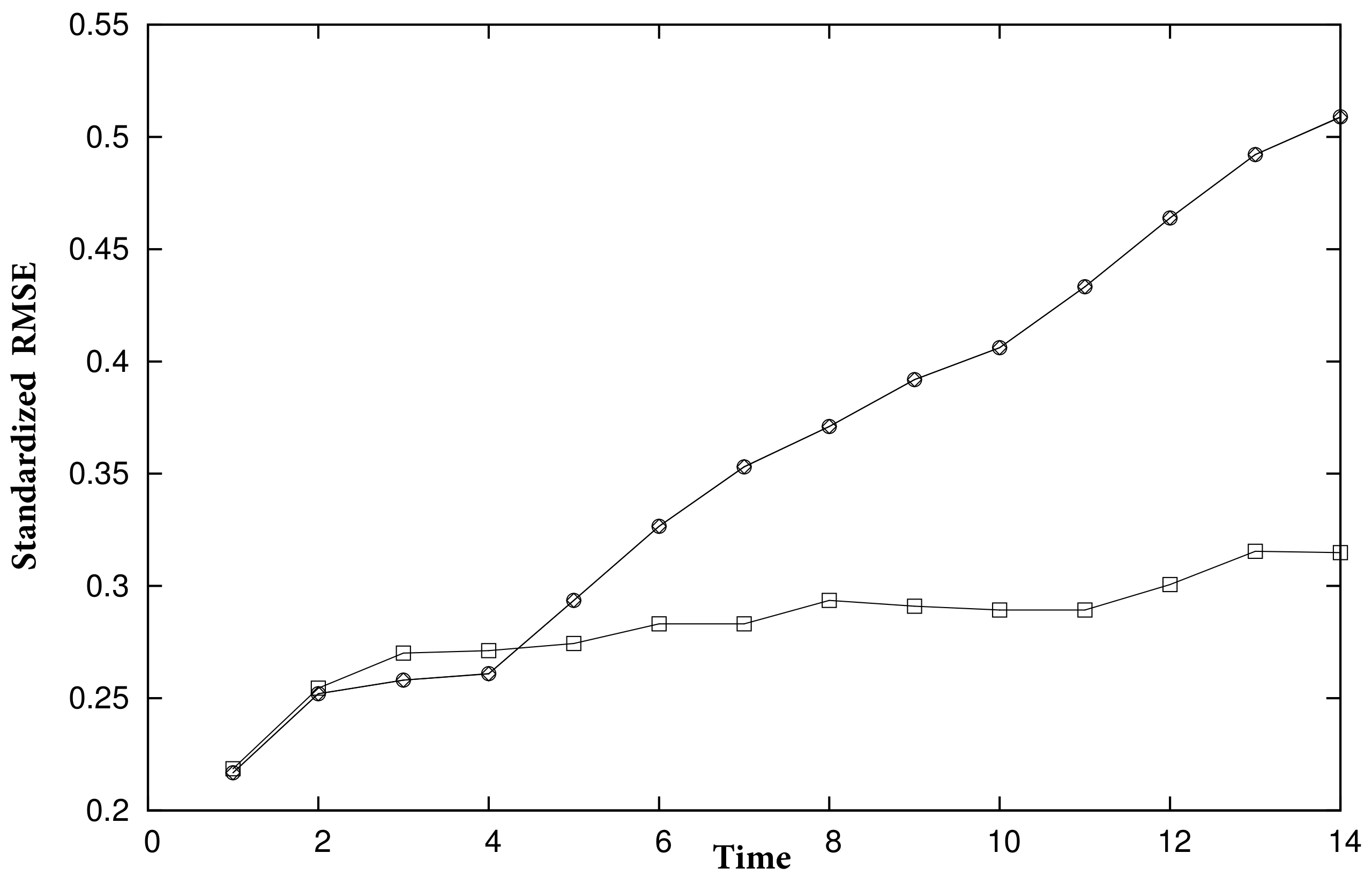
14,000	$[27,37]$	$0.049539$	$0.999453$

shows each value of $\epsilon$, the $\Delta n$ interval where the lines were fitted to $S(\Delta n)$, the maximal Lyapunov exponent, and the correlation coefficient.

Table 3. Maximal Lyapunov exponents for coop2.

$\mathit{\epsilon }$	Range $\mathbf{\Delta }\mathit{n}$	Exponent	Coefficient
2000	$[38,52]$	$0.049485$	$0.999835$
4000	$[34,44]$	$0.049351$	$0.999968$
8000	$[32,45]$	$0.046593$	$0.999930$
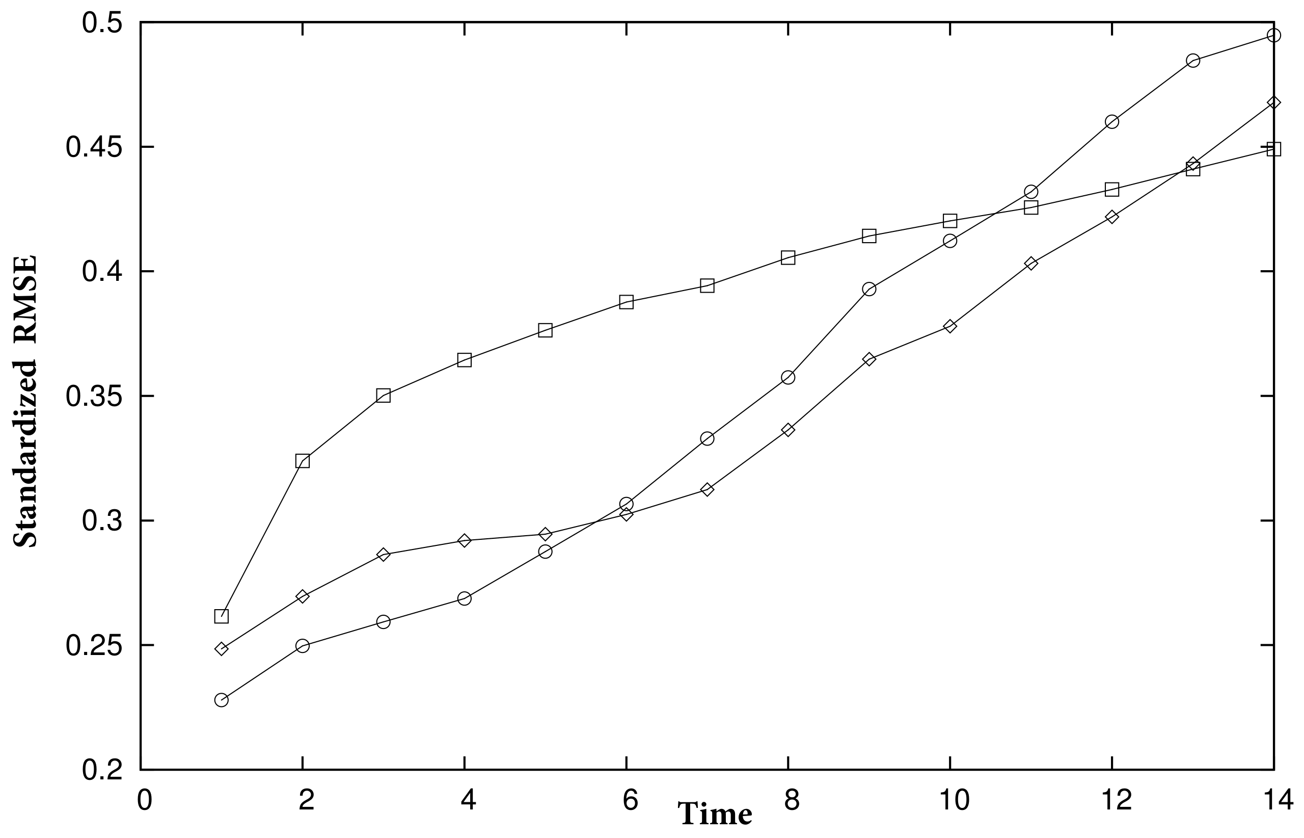
16,000	$[30,44]$	$0.044334$	$0.999872$

and

Table 4. Maximal Lyapunov exponents for coop3.

$\mathit{\epsilon }$	Range $\mathbf{\Delta }\mathit{n}$	Exponent	Coefficient
1000	$[46,74]$	$0.040654$	$0.999546$
2000	$[44,69]$	$0.040315$	$0.999373$
4000	$[43,71]$	$0.038884$	$0.999604$
8000	$[40,70]$	$0.037983$	$0.999479$
12,000	$[36,71]$	$0.036804$	$0.998665$

show the exponents for both coop2 and coop3, respectively. We used delays of 2 and 1 day, respectively, and the curves corresponding to dimension 10.

Since the series are non-stationary, we performed additional checks to ensure that the exponent was correct. First, we computed the exponent for some parts of each series. We found that the exponents differed to some extent, but there was not a big difference. For coop1, we divided the series into the first four seasons and the last six seasons, which seemed to be stationary. Results are shown in

Table 5. Maximal Lyapunov exponents for coop1 subseries.

First 4 Seasons
$\mathbf{\epsilon }$	Delay	Range $\Delta \mathit{n}$	Exponent	Coefficient
2500	2	$[37,60]$	$0.033932$	$0.999293$
5000	2	$[37,53]$	$0.042953$	$0.999331$
7000	2	$[38,53]$	$0.042915$	$0.998767$
9000	2	$[40,50]$	$0.044363$	$0.996814$
14,000	2	$[39,44]$	$0.052637$	$0.998350$
Last 6 Seasons
$\mathbf{\epsilon }$	Delay	Range $\Delta \mathit{n}$	Exponent	Coeficient
2500	2	$[34,60]$	$0.036119$	$0.999693$
5000	2	$[27,52]$	$0.039526$	$0.999682$
7000	2	$[24,51]$	$0.038135$	$0.999653$
9000	2	$[25,48]$	$0.036410$	$0.999531$
14,000	2	$[22,41]$	$0.036882$	$0.999364$

. For coop2 (

Table 6. Maximal Lyapunov exponents for coop2 subseries.

First 4 Seasons
$\mathbf{\epsilon }$	Delay	Range $\Delta \mathit{n}$	Exponent	Coefficient
2000	2	$[38,55]$	$0.051889$	$0.999930$
4000	2	$[37,48]$	$0.049883$	$0.999755$
8000	2	$[35,51]$	$0.048558$	$0.999732$
16,000	2	$[31,44]$	$0.049202$	$0.999739$
Last 6 Seasons
$\mathbf{\epsilon }$	Delay	Range $\Delta \mathit{n}$	Exponent	Coeficient
2000	2	$[45,70]$	$0.034716$	$0.999751$
4000	2	$[41,61]$	$0.035169$	$0.999702$
8000	2	$[38,57]$	$0.034492$	$0.999950$
16,000	2	$[36,49]$	$0.032439$	$0.999622$

), we chose the first four seasons and the last four seasons. For coop3, we chose seasons 1–3, 4–6, 1–4 y 1–5 (

Table 7. Maximal Lyapunov exponents for coop3 (first and second half).

Seasons 1–3
$\mathbf{\epsilon }$	Delay	Range $\Delta \mathit{n}$	Exponent	Coefficient
1000	3	$[44,77]$	$0.043092$	$0.998316$
2000	3	$[41,73]$	$0.043402$	$0.998516$
4000	3	$[38,71]$	$0.042802$	$0.998661$
8000	3	$[33,63]$	$0.042343$	$0.998135$
12,000	3	$[30,61]$	$0.040764$	$0.998190$
Seasons 4–6
$\mathbf{\epsilon }$	Delay	Range $\Delta \mathit{n}$	Exponent	Coefficient
1000	2	$[60,97]$	$0.029172$	$0.999118$
2000	2	$[57,91]$	$0.030104$	$0.999720$
4000	2	$[52,85]$	$0.029541$	$0.999602$
8000	2	$[50,81]$	$0.029783$	$0.999707$
12,000	2	$[45,79]$	$0.029731$	$0.999593$

and

Table 8. Maximal Lyapunov exponents for coop3 (seasons 1–4 and 1–5).

Seasons 1–4
$\mathbf{\epsilon }$	Delay	Range $\Delta \mathit{n}$	Exponent	Coefficient
1000	2	$[42,69]$	$0.041033$	$0.996666$
2000	2	$[40,69]$	$0.041306$	$0.997620$
4000	2	$[38,69]$	$0.040852$	$0.999009$
8000	2	$[35,69]$	$0.039491$	$0.998923$
12,000	2	$[33,69]$	$0.038913$	$0.998336$
Seasons 1–5
$\mathbf{\epsilon }$	Delay	Range $\Delta \mathit{n}$	Exponent	Coefficient
1000	1	$[45,69]$	$0.039694$	$0.999392$
2000	1	$[43,69]$	$0.039060$	$0.999476$
4000	1	$[43,69]$	$0.037576$	$0.999617$
8000	1	$[41,69]$	$0.036650$	$0.999072$
12,000	1	$[39,69]$	$0.036414$	$0.998659$

). Since these series are shorter than the whole series and thus noisier, sometimes we chose a different delay than the whole series to obtain a longer range of linear increase.

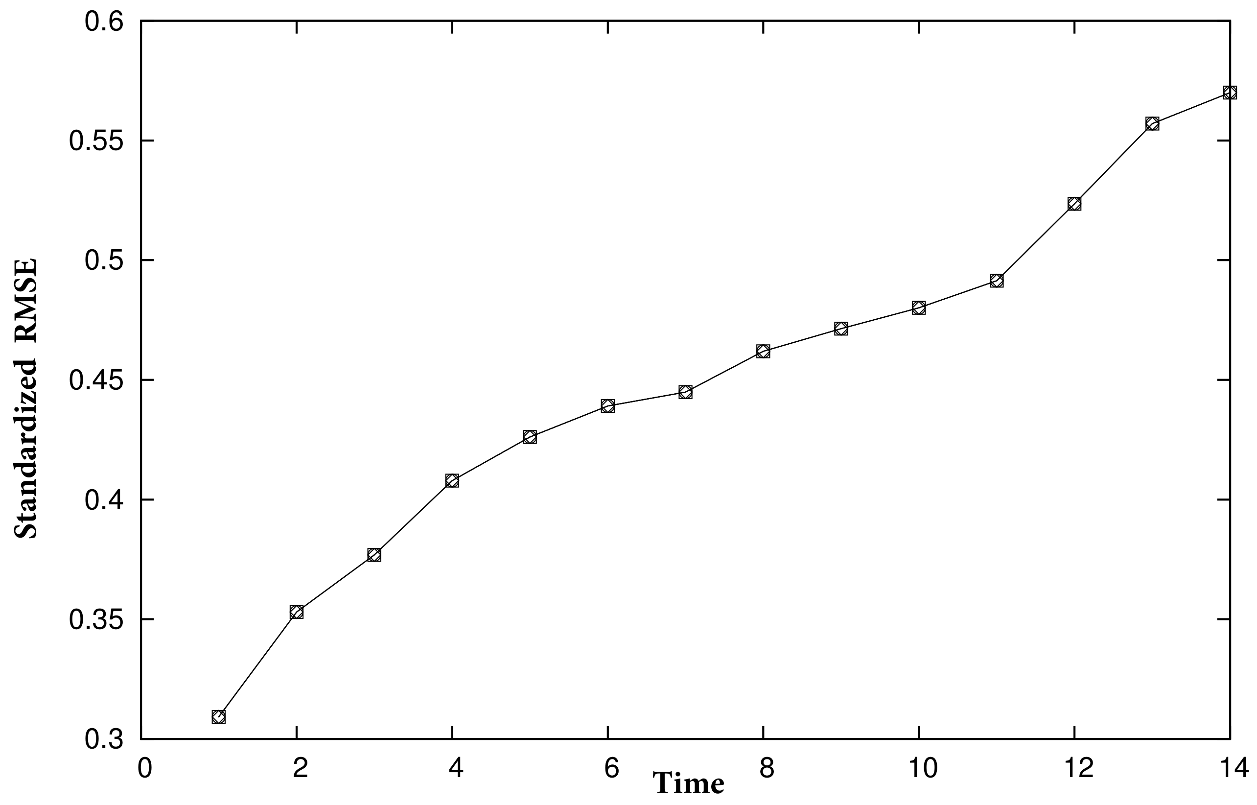
Next, we computed the maximal exponent for the series of the differences. The results are shown in

Table 9. Maximal Lyapunov exponents for coop1 (differences).

$\mathit{\epsilon }$	Range $\mathbf{\Delta }\mathit{n}$	Exponent	Coefficient
1000	$[44,77]$	$0.025899$	$0.998097$
2000	$[42,73]$	$0.028804$	$0.999045$
4000	$[39,65]$	$0.030844$	$0.999562$
8000	$[36,59]$	$0.032047$	$0.999483$
12,000	$[33,54]$	$0.034171$	$0.998611$

,

Table 10. Maximal Lyapunov exponents for coop2 (differences).

$\mathit{\epsilon }$	Range $\mathbf{\Delta }\mathit{n}$	Exponent	Coefficient
500	$[66,89]$	$0.030747$	$0.999539$
1000	$[60,87]$	$0.028890$	$0.998904$
2000	$[54,81]$	$0.028803$	$0.999281$
4000	$[48,73]$	$0.028493$	$0.999873$
8000	$[47,69]$	$0.027050$	$0.999313$
12,000	$[45,60]$	$0.027428$	$0.999044$

and

Table 11. Maximal Lyapunov exponents for coop3 (differences).

$\mathit{\epsilon }$	Range $\mathbf{\Delta }\mathit{n}$	Exponent	Coefficient
250	$[57,87]$	$0.037408$	$0.999269$
500	$[55,83]$	$0.036858$	$0.998921$
1000	$[51,79]$	$0.037610$	$0.999470$
2000	$[48,75]$	$0.037513$	$0.999424$
4000	$[45,71]$	$0.035340$	$0.998392$

. For these series, we fitted the lines to the curves corresponding to dimension 13. In all cases, we used a delay of 2 days.

Finally, we can estimate the noise level from the graphs of $S(\Delta n)$. In Figure 10, we observe a sharp increase at the beginning of the curve for $\epsilon =2500$ that is not present in the other curves. This is probably due to measurement noise. Indeed, when $\epsilon$ is of the order of the noise level, some points that are inside the balls of radius $\epsilon$ would be outside the balls if the noise were suppressed. Then, their real distance is larger than $\epsilon$, so they seem to diverge faster than the other points in the balls, increasing the slope. After some time steps, an exponential divergence of distances due to chaos dominates over noise, and the slope decreases. Thus, the noise level for coop1 is probably around 1000. Applying the same method to coop2 and coop3, we obtained similar noise levels.

3. Results

In the field of predictability research, the non-linear local Lyapunov theory also involves analogs [23,24,25] to model predictive systems [60,61,62,63,64].

Given a series $s_1,\dots ,s_k$, we construct a new series ${\mathbf{s}}_1,\dots ,{\mathbf{s}}_l$ in m-dimensional Euclidean space by time-delay embedding, using a delay of d days [51,57,58]. To predict the behavior of the series $\Delta n$ days ahead of day i, we choose a small $\epsilon >0$ and define

$$P_i(\Delta n)=\frac{1}{\left|\mathcal{U}\right({\mathbf{s}}_i\left)\right|}\sum _{{\mathbf{s}}_j\in \mathcal{U}\left({\mathbf{s}}_i\right)}{\mathbf{s}}_{j+\Delta n}$$

(1)

where $\mathcal{U}\left({\mathbf{s}}_i\right)$ is the set of the points ${\mathbf{s}}_j$ of the sphere of radius $\epsilon$ centered at ${\mathbf{s}}_i$ such that j is less than $i-\Delta n$ (so that we know ${\mathbf{s}}_{j+\Delta n}$) and less than $i-q$, where q is large enough to prevent temporal correlations between ${\mathbf{s}}_j$ and ${\mathbf{s}}_i$. The radius should be as small as possible but above the noise level. Furthermore, there should be enough points in $\mathcal{U}\left({\mathbf{s}}_i\right)$ to prevent strong statistical fluctuations. Thus, we choose a threshold h and, if there are less than h points in the sphere, we increase the radius for that sphere until it contains at least h points.

We split the series into two parts: the first part is used to obtain appropriate parameters for the forecasting model, and the second part is used for a comparison of the real data to the forecasts obtained from the model. In this case, for each series, we chose the second part to be the last season and the first part to be the rest of the series.

The threshold q can be determined from the autocorrelation function. Thus, we have only four adjustable parameters: the dimension m, the delay d, the radius $\epsilon$, and the minimum number of points h. To determine these parameters for each series, we performed predictions from 1 to 14 days in the future for every day in the second-last season and for some ranges of parameters. Next, we determined by least-squares the combination of parameters that produces the smallest errors in the first week, and the same for the second week and the two weeks. Thus, for each series, we obtained three sets of parameters.

The chaotic paradigm states that, despite the noisy appearance of the original series, a correct adjustment of the immersion dimension m will give rise to a complex configuration in phase space known as a strange attractor. These attractors, far from being randomly distributed, have deterministic geometric and dynamic characteristics [65].

For all the series, dimensions [59] were in the range 3–10, the delay ranged from 1 and 14, and the minimum numbers of points were 10, 16, and 22. For coop1, the radiuses were 2000, 3250, 4500, 5750, 7000, 8250, 9500, 10,750, and 12,000. For coop2, the radiuses were 200, 925, 1650, 2375, 3100, 3825, 4550, 5275, and 6000. For coop3, the radiuses were 600, 1525, 2450, 3375, 4300, 5225, 6150, 7075, and 8000. The best parameters for coop1, coop2 and coop3 are listed in the

Table 12. Best parameters for coop1.

Days	Dimension	Delay	Radius	Threshold
1–7	4	4	7000	16
8–14	10	10	7000	22
1–14	4	4	3250	16

,

Table 13. Best parameters for coop2.

Days	Dimension	Delay	Radius	Threshold
1–7	10	3	3825	22
8–14	5	13	1650	16
1–14	7	6	6000	22

and

Table 14. Best parameters for coop3.

Days	Dimension	Delay	Radius	Threshold
1–7	9	10	600	10
8–14	9	10	600	10
1–14	9	10	600	10

, respectively.

Finally, we used these parameters to perform predictions for each series’ last season and to compute the errors. In detail, for each day in the last season, we forecasted two weeks in the future; that is, for day i and prediction horizon $\Delta n$, we made a prediction $P_i(\Delta n)$ for day $i+\Delta n$. Then, for each $\Delta n$, we computed the root mean squared error $P_i(\Delta n)-s_{i+\Delta n}$, where $s_{i+\Delta n}$ is the real data from the series, and we divided it by the standard deviation of the last season’s data. We summarize the results in Figure 12, Figure 13 and Figure 14. Lines with circles correspond to the parameters for days 1 to 7, lines with squares correspond to days 8 to 14, and lines with diamonds correspond to days 1 to 14.

4. Discussion and Conclusions

We studied three time series of daily strawberry production data for an interval of between 6 and 10 years. We discovered that the system is chaotic and therefore, even if the data were stationary, linear methods such as Box–Jenkins could not have been applied.

First, we detected that the power spectra were all broadband, which is consistent with chaos. Then, we studied the system’s sensitivity to the initial conditions (exponential growth of the errors) using the maximal Lyapunov exponent (a metric model that studies the growth of the distances between points of a strange attractor). To confirm the validity of its calculation in short and non-stationary series, we used over-immersion and repeated the calculation in sections of the series and transformed series.

Applying non-linear methods, such as the maximal Lyapunov exponent computation, we observe ranges of exponential divergence of the distances, with maximal Lyapunov exponents around 0.04. The Fourier analysis also shows the cyclical influences of the weekday and the season. We also tried to compute the correlation dimension. However, we did not obtain clear results, and we conjectured that the quasi-periodic influence of the weekday and the season introduce strong temporal correlations that require longer time series to compute a significant dimension. Finally, we estimate that the non-deterministic noise is around 1000. We made forecasts for the last season of the series and compared the real data results, obtaining an appropriate model for short-term prediction.

The results indicate that power spectra and the maximal Lyapunov exponent can be used as effective methods to judge chaos characteristics [18,19]. We also conclude that non-linear models are more suitable than linear models for the study of strawberry harvest prediction in these companies, and that there is possibly a small-dimension attractor in this dynamic system.

In the methodology described in this work, the existence of predictable structures is also contrasted for each observation, since the unpredictability of an observation of the series from the rest reveals the independence of the random variable that generates it with respect to the rest and hence white noise, and predictability reveals non-linear determinism and therefore chaos. Thus, with the production series, we have made local predictions for analogous occurrences.

This deterministic and non-stochastic chaotic series has the characteristic that short-term prediction is possible, while medium and long-term prediction is not possible with a high degree of reliability. The practical implication from an economic perspective is the impossibility of making long-term predictions that can reorient the company’s productive policy or the sector. However, short-term predictions will support the logistics and commercial operations of a company and therefore the product profitability. The use of machine learning techniques that try to find internal structures with the predictive power of certain characteristics of the series in the long term, instead of a detailed behavior in the short term, thanks to deterministic chaos is perhaps a future objective to be investigated. However, this requires a much longer data series than we currently have.

Another step to study will be to incorporate other variables into the model to verify if the predictive result improves and determine the bifurcation points that will alert us to the risks of catastrophes that may change the dynamics of the model.

Finally, in order to simplify the computational part of the resolution to our problem, we have discarded other recent algorithms that identify implicit non-linearities or non-linear systems reconstruction techniques on non-stationary chaotic data since the main idea of our work was to find a simple solution to the stationarity problems encountered. For example, if we apply the SINDy method [11], we must consider many non-linear functions within the matrix of possible functions, which makes it computationally difficult. On the other hand, we have obtained good results without having to rebuild the time series, such as in [16], making the method lighter, although certainly less successful. However, we leave these objectives as some very interesting future lines of research that can potentially improve upon the typical linear research carried out on the modeling of primary sector activities.