Article

Deep Gene Networks and Response to Stress

by
Sergey Vakulenko
1,*,† and
Dmitry Grigoriev
2,†
1
Saint Petersburg Electrotechnical University “LETI”, 197376 Saint Petersburg, Russia
2
CNRS, Mathématiques, Université de Lille, 59655 Villeneuve d’Ascq, France
*
Author to whom correspondence should be addressed.
These authors contributed equally to this work.
Mathematics 2021, 9(23), 3028; https://doi.org/10.3390/math9233028
Submission received: 13 October 2021 / Revised: 18 November 2021 / Accepted: 23 November 2021 / Published: 26 November 2021
(This article belongs to the Special Issue Application of Mathematical Methods in Artificial Intelligence)

Abstract

:
We consider systems of differential equations with polynomial and rational nonlinearities and with a dependence on a discrete parameter. Such systems arise in biological and ecological applications, where the discrete parameter can be interpreted as a genetic code. The genetic code defines system responses to external perturbations. We suppose that these responses are defined by deep networks. We investigate the stability of attractors of our systems under sequences of perturbations (for example, stresses induced by environmental changes), and we introduce a new concept of biosystem stability via gene regulation. We show that if the gene regulation is absent, then biosystems sooner or later collapse under fluctuations. By a genetic regulation, one can provide attractor stability for large times. Therefore, in the framework of our model, we prove the Gromov–Carbone hypothesis that evolution by replication makes biosystems robust against random fluctuations. We apply these results to a model of cancer immune therapy.

1. Introduction

In this paper, we consider systems of differential equations with polynomial and rational nonlinearities and with a dependence on a discrete parameter (hybrid systems). Such systems arise in biological and ecological applications, where the discrete parameter allows us to incorporate in the model a genetic regulation by a genetic code. We investigate the stability of attractors of these systems under stress. The attractors define system functioning regimes, while stresses are sudden changes of system parameters (for example, heat shocks). Our aim is to investigate the attractor stability under infinite sequences of shocks. It is inspired by the following idea of M. Gromov and A. Carbone: “Homeostasis of an individual cell cannot be stable for a long time as it would be destroyed by random fluctuations within and out of cell. There is no adequate mathematical formalism to express the intuitively clear idea of replicative stability of dynamical systems” ([1], p. 40). It is clear that replicative stability is important for the evolution of cancer cells, viruses, for example, such as COVID 19, and bacteria such as E. coli. There is no doubt that replication helps viruses and bacteria survive in changing environments (see, for example, Lensky’s experiment with E. coli [2]). However, there is a non-trivial question: how to estimate chances that such replicative evolution can continue eternally even under action of therapeutic agents? For COVID-19, it is an important question of will we have fourth or fifth pandemic waves, etc., or can the virus vanish? In this paper, however, we consider cancer cells as an example because our analyses are more applicable to this case.
Using a model, proposed in this paper, one can formulate the Gromov–Carbone idea in rigorous mathematical terms and, under some assumptions, to prove this hypothesis. Our model exploits ideas of artificial intelligence theory; namely, we suppose that the response to stress is defined by deep gene networks (DGN), which are similar to deep neural networks (DNNs). It allows us to use estimates obtained recently in DNN theory [3,4,5]. Note that deep networks were recently applied as interpretable models of the gene network regulations in [6].
To describe replicative stability, we incorporate into our model a regulation by the discrete parameter (for biosystems and ecosystems it is a gene regulation) and consider how the stochastic stability depends on regulation. Our results help us to explain, for example, why cancer cells exhibit a long survival time even under a strong therapy. Indeed, cancer cells give us an example of evolving biosystem affected by a sequence of stresses (for example, immune therapy or chemotherapy). It is worth noting that replicative stability for biochemical systems, introduced in this paper, is a new idea for the theory of stability (robustness) of these systems. Earlier, a number of works (see fundamental papers [7,8] and references therein) considered a more usual approach, which investigates reactions of the biochemical system to the small disturbances of kinetic rates or reagent concentrations. We also investigate the stability in the vicinity of small changes in some states (attractors). However, we take into account variations of the system genotype. We suppose that these variations compensate for a significant part of external perturbations that reinforces the system stability. The gene regulation system evolves in such a way that this compensation mechanism becomes more and more effective, which provides stability under fluctuations for large times.
Let us first outline the concept of stochastic stability. We consider organisms as biochemical machines, which can be modeled by a system of ordinary differential equations. A regime of our biosystem functioning is defined by an attractor A . Let us denote by P δ , A , τ the probability that the system state lies in a δ -neighborhood of the attractor A within the time interval [ 0 , τ ] . The parameter δ > 0 defines the size of a homeostasis domain, where the system stays viable (here we follow viability theory, see, for example, [9]). In the framework of that viability approach, the Gromov–Carbone hypothesis reduces to two claims. The first assertion is that for biological systems with fixed parameters and a fixed genetic code,
P δ , A , τ 0 a s τ + .
This means that all biosystem states, sooner or later, will be destroyed by fluctuations. The second assertion is that a sequence of modifications of the system genotype can lead to eternal stability, where the viability probability stays positive for all times:
P δ , A , τ > β > 0 τ > 0 ,
where β > 0 . The constant β can be interpreted as follows: imagine a large population of cancer cells, bacteria or viruses. Let this population be affected by consecutive therapeutic attacks. The constant β describes the relative fraction of cells ( bacteria, viruses) that will survive.
In other words, systems with fixed parameters are unstable under environment fluctuations but the evolution of the genetic code can stabilize them. This replicative stability is considered in [10] for some network models; see [11] for an overview. For some classes of hybrid dynamical systems involving a dependence on discrete genotypes s ( t ) , which can evolve in time, it is shown that inequality (2) implies
sup t [ 0 , T ] L ( s ( t ) ) + T ,
i.e., the genotype length L has a tendency to increase. Here we assume that the genotype s is a Boolean string ( s 1 , . . . , s N ) and the length L of s is N. However, it is well known that the genotype length does not correlate directly with the morphological complexity and that evolution does not always lead to a genotype length increase. For example, Drosophila, nematode and human have numbers of coding genes of the same order (although bacteria genomes are much shorter than the nematode genome). Nonetheless, it is well known that the gene regulation system has become more and more complex throughout evolution. In this paper, we use deep networks (DNs) to describe gene regulation and show that DN network growth makes biosystems stable for long time periods.
Let us outline the model in more detail. In contrast to some earlier works [12,13,14], which used either formidable computations [12,13], or sophisticated nonlinear asymptotics [14], we use deep networks. These networks consist of, in general, many layers. The depth L = L n e t of a network is the number of hidden layers, and the size S = S n e t is the total number of units. In practice, networks with depth L n e t = O ( 1 ) can be considered as shallow, while deep networks typically have many layers. Connections between units in these networks depend on coding sequences s = ( s 1 , , s N ) , s i { 0 , 1 } of Boolean genes, which could be switched off ( s i = 0 ) or switched on ( s i = 1 ). The inputs of the DN’s are the stress parameter values and the system states. The DN produces an output, which depends on unit interconnections and thus on the genetic code, which determines these interconnections. The main idea behind our model of regulation is that the DN output and the stress impact cancel out each other.
To describe stress impacts, we use a model of subsequent environmental shocks. This idea is consistent with the Gould–Eldredge concept [15], where evolution is represented as a sequence of intermittent short bursts and longtime stasis periods, the evolution bursts appear in response to stresses induced by environment. Let τ 1 , τ 2 , . . . , τ k , . . . be an infinite increasing sequence of time moments τ j . These moments can be considered as moments of environment shocks (stresses), when the environment suddenly changes. At these moments, some system parameters can change. A well-known example is a heat shock connected with temperature, which affects kinetic rates in biochemical systems and produces mutations [16]. For cancer cells, these shocks can describe a therapy. Our aim is to estimate the probability that a local attractor A is robust under all those environmental shocks within a large (maybe, infinite) time interval.
Let us outline our results. The first result (Theorem 1) concerns a connection between gene regulation complexity and uncertainty of environment. The important measure of genetic regulation complexity is the number of equilibria of gene regulation network N r e g . This question on the number of the equilibria has received the attention of many works; in particular, it was studied for the famous NK model (pioneered in [17]). The NK model is a mathematical model describing a “tunably rugged” fitness landscape, depending on two parameters, N and K. The parameter N is the length of a Boolean genotype s length, and K defines the topology of fitness landscape via the number of genes involved in the trait control. The NK model has the main applications in evolutionary biology. First, it was supposed that N r e g is a relatively small, N r e g N κ , where an exponent κ > 0 . In particular, for the Hopfield model with symmetrical interaction [18], this relation holds with κ = 1 . However, later it was shown that in the NK model, N r e g can be exponentially large [19]. A similar result is obtained for another simple model, which describes a special class of Hopfield models with asymmetric interaction and a special interaction topology [20]. Experimental data [21,22] show that in gene interaction networks there are strongly connected nodes that can be named hubs, or centers. The hubs communications go via a number of weakly connected nodes. This centralized connectivity has been found in gene–gene and protein–protein interaction networks [21,22], and such networks can support many equilibrium states.
To explain why they have a number of equilibria, we define an entropy H e x t , δ of environment uncertainty, depending on the robustness level δ and gene regulation. This quantity is the Kolmogorov δ -entropy (see, for example, [23,24]) on the metric space of perturbations ξ with a special metric. We show that if an attractor describing biosystem functioning does not collapse under all perturbations (conserves its topological structure) then there exists a connection between N r e g and the entropy H e x t , δ :
log 2 N r e g H e x t , δ .
This means that entropy of regulation must be no less than the environment uncertainty.
This result, in particular, shows that, to kill cancer cells, we should use a combined therapy (for example, chemotherapy together with a heat therapy). Hyperthermia therapy is heat treatment for cancer that can be a powerful tool when used in combination with chemotherapy or radiation. Chemotherapy resistance develops over time as the tumors adapt (due to replicative stability). Chemoresistance against several anticancer drugs could be reversed by the addition of heat therapy.
Our results show that before all, it is necessary to attack hubs of the gene regulation network. In fact, N r e g critically depends on the gene interaction topology. Even a small increase in the number of hubs in gene regulation networks leads to a sharp increase in N r e g [20]. These results are consistent with the conclusions of [25,26], where it was shown that network hubs buffer environmental variations and also make switches in regulatory networks. Our results are supported by some experimental data, at least qualitatively [27]. A number of hub genes are identified in cancer cell regulation. According to these results, drugs attacking the hub genes should be especially effective. A list of such candidate drugs targeting hub genes can be found in Table 3 from [27].
There is also a connection with basic results of hard combinatorial problem theory. Fundamental results [28] on Boolean functions and the K-SAT problem assert that to satisfy many constraints, we should use a number of Boolean variables. Our result (4) can be considered as an analog of these results. If we have a genotype s of the length N, then log 2 N r e g N ; thus, for Boolean regulation models, (4) implies that the genome length N should be more than the entropy H e x t , δ .
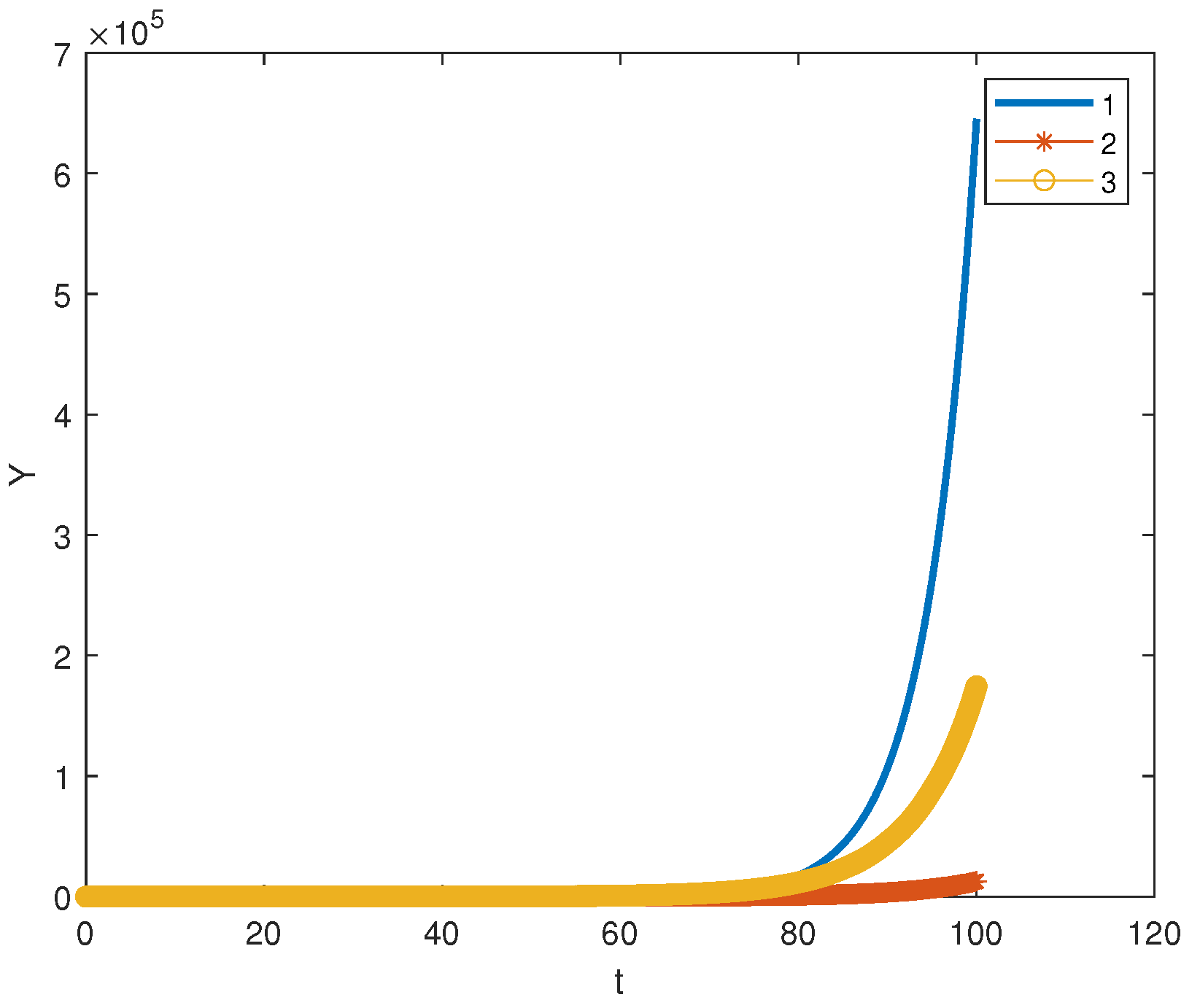
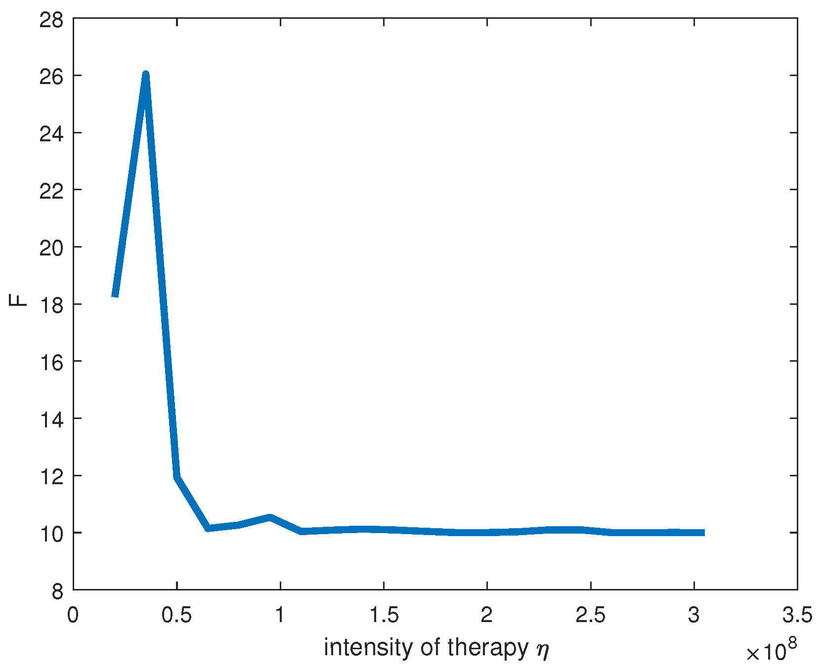
Furthermore, we show that it is possible to provide stochastic attractor robustness by an appropriate genotype choice at each environment shock τ 1 < τ 2 < . . . . If, in contrast, the genotype is fixed, then the stochastic stability tends to zero as τ + . For cancer these results are confirmed by numerical simulations, where we use a model from [29] extended to take into account the evolution of cancer cells. If the cancer cells do not evolve, immune therapy may be effective, otherwise cancer wins sooner or later.
To conclude this introduction, let us note that the estimates of stochastic stability, obtained in the paper (see Theorem 3), allows us to find the main factors, which determine the organism fate under the stress stability: the sparsity of reaction network, the stress sensitivity, the stress dimension (the number of perturbed external parameters affecting the rates of biochemical reactions) and the size of gene regulation network.
The paper is organized as follows. In the next section, we describe models with random perturbations and gene regulation. In Section 4, we state the model of environmental shocks and formulate some assumptions needed for the mathematical tractability of the problem. In Section 5, we formulate some definitions, and further, we find a necessary condition for the attractor stability.
In Section 7, we consider attractor robustness under a sequence of environment shocks. In this section, we apply DNN’s that finally give Theorem 3, which states an estimate of replicative stability. The last section contains a discussion and conclusions. To simplify reading, the technical parts of demonstrations are relegated into Appendix A.

2. Materials and Methods

We use standard methods of mathematical analysis and theory of differential equations. Moreover, we apply the known results for approximations of Lipshitz smooth functions by deep neural networks [3,4,5]. For numerical simulations, and to produce Figure 1, we used Matlab and the standard Euler method.

3. Model with Random Parameters

We describe our models in two steps, first we formulate a model without gene regulations and then with regulation.
We consider systems of differential equations with a dependence on a random process ξ ( t ) . They have the form
d v d t = f ( v , ξ ( t ) ) t 0 ,
where v ( t ) = ( v 1 ( t ) , , v n ( t ) ) t r D , where D is a compact domain in R n with a smooth boundary D , v i ( t ) are biochemical species concentrations, f ( v , ξ ) = ( f 1 ( v , ξ ) , , f n ( v , ξ ) ) t r , the reaction terms f i are sufficiently smooth functions of v, for example, multivariate polynomials in v, and also smooth functions of ξ R p . The functions ξ ( t ) are random processes of a trajectory, which are piecewise constant in t and take values in a compact subset P e x t of R p , where the quantity p is a positive integer (dimension of stress parameter ξ ). These processes ξ ( t ) describe multiplicative noise. The source of this noise is an environment of a biosystem. Other assumptions of ξ ( t ) will be described later.
We complement the system of stochastic Equation (5) by initial conditions
v ( 0 ) = v ( 0 ) .
To define f we use the standard models of chemical kinetics and population dynamics. The simplest choice is a polynomial model, which can be derived by the law of mass action:
f i ( v , ξ ) = a R i C i , a ( ξ ) v 1 a 1 v 2 a 2 . . . v n a n ,
where a = ( a 1 , . . . , a n ) is a multi-index with integers a i 0 , R i are finite subsets of I n = { 1 , , n } and C i , a are coefficients that determine kinetic rates. Note that the well-known Lotka–Volterra and generalized Lotka–Volterra systems (which have ecological and economical applications, see [31,32]) are also included in the class of systems defined by (7).
In real biochemical applications, we are often dealing with binary reactions, where only two exponents a i 0 , and sparse f i , where, although the reagent number n may be large, for each i, the number m i of non-zero coefficients C i , a in each row is bounded, m i < < n . In a more sophisticated case (which arises when in a slow-fast polynomial system we express fast variables via slow ones) we have rational v nonlinearities, for example,
f i ( v , ξ ) = a R i C i , a ( ξ ) P i , a ( v ) Q i , a ( v ) ,
where P i , a ( v ) and Q i , a ( v ) are polynomials. We suppose that Q i , a ( v ) are separated from zero:
| Q i , a ( v ) | > δ 0 > 0 ,
for all i , a and v D . Such systems appear in biochemical kinetics, population dynamics and cancer modeling. As an example, let us consider the following model of cancer immunotherapy [29,30]:
d v 1 d t = r 0 + ρ v 1 v 2 α + v 1 c 1 v 1 v 2 d 1 v 1 + ξ ( t ) ,
d v 2 d t = r v 2 ( 1 b v 2 ) c 2 v 1 v 2 ,
where v 1 denotes the concentration of cells with antitumor activity in the tumor site (CTL cells), and v 2 is the concentration of tumor cells. This model thus concerns two cell populations: normal cells and cancer ones. Parameters r 0 , c 1 , c 2 , b , r , d 1 , α , ρ are positive coefficients, which can be explained as follows. The parameter r 0 is the normal rate of immune cell flow into the tumor site, c 1 is the immune cells death rate due to interaction with tumor cells, c 2 is the fraction of tumor cells killed by immune cells, 1 / b is the tumor cells carrying capacity, r is the tumor cells growth rate, d 1 is a natural death rate of immune cells, α is the steepness coefficient of immune cell recruitment and ρ is the maximal immune cells recruitment rate [29]. For ξ ( t ) 0 this model and its generalizations are investigated in [30], the term ξ ( t ) describes a therapy by infusion of CTL cells (it is proposed in [29]).
To provide the existence and uniqueness of solutions to the Cauchy problem (5) and (6) for all t ( , ) , we assume the following. Let
f ( v , ξ ) · n ( v ) 0 v D ξ P e x t
where n ( v ) is a unit normal vector directed outside D at the point v D . Then solutions of the Cauchy problem (5) and (6) exist and are unique for all t > 0 .
It is worth noting that polynomial and rational functions f i may not satisfy conditions (12). Since we further investigate a local stability of local attractors, we can restrict ourselves to considering narrow neighborhoods of those attractors A . Therefore, we can truncate nonlinearities in f i ( v ) setting for instance f ˜ i ( v ) = f i ( v ) χ A ( v ) , where χ A ( v ) 0 outside of an open neighborhood W of A .

3.1. Extended Model with Regulation

Different complicated models of gene regulation were proposed, for example, [33,34] for Drosophila morphogenesis, however, we apply another approach using DNN’s and inspired by recent biological works (for example, [6]).
Let s ( t ) = ( s 1 ( t ) , . . . . , s N ( t ) ) be a time dependent gene expression vector. We have N Boolean genes s i , which take values in the set S N = { 0 , 1 } N , s i { 0 , 1 } . The i-th gene may be switch on (when s i = 1 ), or switch off (when s i = 0 ). The Boolean string s encodes interconnections in the networks of gene regulation (see Section 7.2). We incorporate genes s into system (5) using the following
Assumption GRSuppose that coefficients C i , a depend on the genetic code s:
C i , a = C i , a ( ξ , s )
and they are Lipshitz in ξ for each s.
This assumption means that regulation goes via a genetic control of kinetic rates. Moreover, we assume that the network finds a genotype s, which produces an optimal answer to stress, almost instantly. We obtain thus that s is involved in the vector field f ( v , ξ ) via kinetic coefficients C i , a : f = f ( v , ξ , s ) .
Let us introduce vector fields describing perturbations. Consider, for example, a heat shock. All kinetic rates depend on the temperature T: C i , a = C i , a ( T ) , sometimes in a complicated manner. However, typically we have a reference value T = T ¯ corresponding to an optimal functioning regime (for example, if T is the human body temperature, then T ¯ is about 36 degrees). Let T = T ¯ + Δ T , where Δ T is a temperature increment corresponding to a heat shock. Then in the case (7) one obtains that the perturbations g i of the f i have the form
g i ( v , T , s ) = a R i C ˜ i , a , s v 1 a 1 v 2 a 2 . . . v n a n ,
where
C ˜ i , a , s = C i , a ( T ¯ + Δ T , s ) C i , a ( T ¯ , s ) .
In the general case, let ξ ¯ be an optimal parameter value corresponding to a normal system functioning. Then we denote by
g ( v , ξ , s ) = f ( v , ξ , s ) f ( v , ξ ¯ )
the perturbation of f, which appears as a result of a parameter ξ variation. Let us denote the non-perturbed field f ( v , ξ ¯ ) by f ¯ ( v ) . Then we have the two following systems: the non-perturbed one
d v d t = f ¯ ( v ) ,
and the perturbed system:
d v d t = f ¯ ( v ) + g ( v , ξ ¯ , s )
where, in general case, ξ and s can depend on t.

3.2. Attractors and Semiflows

Let us denote by A s , ξ a compact invariant locally attracting set (a local attractor) of semiflow S s , ξ t generated by the Cauchy problem for system (17) for given fixed s and ξ . The semiflow generated by the non-perturbed system (16) will be denoted by S t and the corresponding attractors by A . We consider mainly two cases: A is a stable hyperbolic equilibrium v e q or a stable hyperbolic limit cycle V ( t ) with a period T 0 . (A reminder that hyperbolicity for an equilibrium means that the spectrum of the corresponding linearized operator does not intersect an imaginary axis, while for cycles it means that the corresponding Floquet multiplicators do not lie on the unit circle of the complex plane. For the general theory of hyperbolic sets, see [35,36]). We are going to estimate the probability that a local attractor (or an invariant set) of our system is stable under those shocks. We define that probability in the next subsection.

4. Stochastic Stability under Shocks

4.1. Environmental Shocks

To describe stresses, we use the model of subsequent environmental shocks. Let τ 1 , τ 2 , . . . , τ k , . . . be an infinite increasing sequence of time moments τ j such that min j ( τ j + 1 τ j ) > > Δ τ > > Δ t , where Δ t and Δ τ are characteristic times of gene regulation functioning and biochemical model dynamics, respectively. At the moments τ j we have environment shocks, when an interaction between the environment and the biosystem changes. We suppose that within interval [ τ j , τ j + 1 ) the parameter ξ = ξ j , where at each step j we choose ξ j randomly as follows in two steps. The first step is a random choice of the set P e x t , j of perturbations affecting the system at j-th interval I j = ( τ j , τ j + 1 ] . We choose the set P e x t , j randomly from a countable set E = { P e x t , 1 , P e x t , 2 , . . . , } . The index k in P e x t , k defines a kind of interaction between the organism and its environment. Each set P e x t , j is equipped with a probabilistic measure μ j .
The second step is a random choice of ξ j P e x t , j . The shocks ξ j are independent, and at each step j and each k, we sample ξ j according to the measure μ j . Therefore, we obtain a sequence of independent random variables ξ j , j = 1 , . . . , + , which describes subsequent random changes of our stress environment.

4.2. Attractor Stochastic Stability

To formulate the stochastic stability problem, we use the viability approach [9]. Let A be an attractor under consideration. For δ > 0 we introduce a small tubular neighborhood of that attractor by
W δ ( A ) = { v : d i s t ( v , A ) < δ } ,
where the distance between a state v and a subset B D is defined as
d i s t ( v , B ) = inf w B | v w | ,
where | v | is the standard Euclidean norm in R n .
Let us introduce probability that the state of our system lies in W δ ( A ) within the time interval [ 0 , τ ] :
P δ , A , τ = P r o b { v ( t ) W δ ( A ) t [ 0 , τ ] } .
Naturally we suppose that the initial value v ( 0 ) W δ ( A ) . The probability P δ , A , τ depends on that initial value. Since our aim to obtain estimates of P δ , A , τ uniform in v ( 0 ) A we will omit dependence on v ( 0 ) . The probability P δ , A , τ can be considered as a measure of attractor A stochastic stability.

5. Robustness with Gene Regulation

5.1. Definitions

Let us formulate certain definitions. We consider ergodic attractors A . The statement of ergodic attractor’s theory can be found in [37]. For such attractors and sets, the time average can be replaced by averages over the attractor taken by an invariant measure ρ defined on the attractor. Let us introduce the time averages along trajectories
ϕ A = lim T + T 1 0 T ϕ ( v ( t ) ) d t
where ϕ ( v ) is a smooth function, and v ( t ) is a trajectory on the attractor. For ergodic attractors these averages exist and do not depend on the choice of the trajectory v ( t , v ( 0 ) ) on the attractor for almost all v ( 0 ) with respect to the measure ρ . Of course rest point and limit cycle attractors are ergodic, but theory [37] also concerns the non-trivial situation, where A may be chaotic.
Let us denote by Φ the set of all smooth functions ϕ defined on D. We denote by L i p ( ϕ ) the Lipshitz constant of ϕ :
| ϕ ( v ) ϕ ( v ˜ ) | L i p ( ϕ ) | v v ˜ | .
Definition 1. 
We say that a local attractor A of the semiflow S t defined by Equation (17) with ξ = ξ ¯ is ε-robust with respect to the stress parameter ξ and the genotype s if
| ϕ A ϕ A s , ξ | < L i p ( ϕ ) ϵ , ϕ Φ ,
i.e., the time averages over the perturbed and unperturbed attractors are ϵ-close.
Note that if the attractor is hyperbolic and ϵ > 0 is small, then due to the persistence of hyperbolic sets [35,36], the perturbed attractor is topologically equivalent to the non-perturbed one.
Definition 2. 
A local attractor A of the non-perturbed flow S t defined by system (16) is ϵ-robust with gene regulation with respect to the stress environment P e x t if for each ξ P e x t there is an appropriate genotype s ¯ ( ξ ) such that
| ϕ A ϕ A s ¯ , ξ | < L i p ( ϕ ) ϵ , ϕ Φ
where A s ¯ , ξ is the local attractor A s ¯ , ξ of the semiflow S s ¯ , ξ t .
Due to the definition of robustness under gene regulation for each field ξ P e x t we have a genotype s ¯ ( ξ ) such that trajectory averages over the perturbed attractor A s ¯ , ξ are ε -close to ones for non-perturbed attractor A of system (16). We have thus the map S : ξ s ( ξ ) S N from the set P e x t into the set of all genotypes S N .

5.2. Robustness Condition

Let us formulate a claim.
Proposition 1. 
Let a local attractor A of a non-perturbed system (16) be ergodic and ε-robust with respect to ξ P e x t and s S N . Then
g ( v , ξ , s ) A < C 1 ϵ ,
where the constant C 1 > 0 is uniform in ϵ > 0 .
Proof. 
We take the averages of the right and left hand sides of Equations (16) and (17) that gives
f ¯ i A = 0 , f ¯ i + g i A s , ξ = 0
for all i. By Definition 1 of robustness one has
| f ¯ i + g i A f ¯ i + g i A s , ξ | < c 0 ϵ ,
where c 0 > 0 are uniform in ϵ > 0 . Then (25) and the last estimate give (24). □

6. Gene Regulation and Robustness

In this section, we describe a connection between robustness and the gene regulation.

Environment Uncertainty

In this subsection, we introduce a measure of external perturbation uncertainty. Let δ > 0 be a number. Consider the set P e x t of perturbations ξ . Let us introduce a special distance between perturbations depending on the attractor and g:
d i s t A , g ( ξ , ξ ˜ ) = min s S N sup i = 1 , . . . , n | g i ( · , ξ , s ) g i ( · , ξ ˜ , s ) A | ,
where S N = { 0 , 1 } N denotes the set of all genotypes.
By C δ we denote a δ -covering of P e x t consisting of the sets B i , δ , i = 1 , 2 , . . . , N c o v e r :
P e x t = j = 1 N c o v e r B j , d i a m ( B j ) δ j ,
where the diameter d i a m ( B ) of a bounded set B is defined by
d i a m ( B ) = sup ξ , ξ ˜ B d i s t A , g ( ξ , ξ ˜ ) .
The formula for the diameter can be rewritten as
d i a m ( B ) = min s S N max i , ξ , ξ ˜ B | C ˜ i , a ( ξ , s ) C ˜ i , a ( ξ ˜ , s ) v a A | .
We define H e x t , δ as the Kolmogorov δ -entropy of P e x t :
H e x t , δ = inf C δ log 2 N c o v e r ,
where we take the infimum over all δ -coverings.
Remark 1. 
The introduced entropy depends on the parameter δ, and decreases in δ > 0 . Moreover, H e x t , δ depends on the unperturbed attractor A (we omit that dependence in our notation).
Remark 2. 
The Kolmogorov δ-entropy has numerous applications for coding, image processing and neural networks, see [23,24].
It is difficult to compute H e x t , δ ; however, we can find a rough estimate of this entropy via the dimension d s t r = d i m ξ of the stress parameter. Suppose that the diameter of P e x t is bounded: d i a m ( P e x t ) R 0 , where R 0 is a positive constant, which can be interpreted as a maximal absolute value of the stress parameter variations. Then we obtain
H e x t , δ d s t r log 2 ( R 0 / δ ) .
If the set P e x t is not compact then H e x t , δ = + .
There holds
Theorem 1. 
Let an ergodic attractor A of a non-perturbed system (16) be ε-robust with gene regulation. Then for sufficiently small ε > 0 one has
log 2 N r e g H e x t , δ
where δ = C ε , where C > 0 is a constant uniform in ε as ε 0 .
For a proof, see Appendix A. The idea is simple: using Proposition 1 one can show that if the same genotype provides the stability for all perturbations from a set B, then d i a m ( B ) < C 1 ϵ .
By results of [20] we can find a connection between the number of centers (hubs) in the gene regulation network and the entropy H e x t , δ . To find a rough estimate, we suppose that we have a starlike network with N c centers and each center is connected to N s satellites. Then the equilibrium number N r e g has the order N s N c = exp ( N c ln N s ) [20] and
log 2 N r e g log 2 exp ( N c ln N s ) = c 0 N c ln N s .
Equation (30) shows that the main factor determining the effectiveness of the gene response to stresses is the number of hubs involved in the corresponding gene regulation, and N c ln N s c o n s t H e x t , δ (we use here that ln is a very slow increasing function of its argument). The estimate (28) then gives the following topological condition of the stability:
N c > c 0 1 log 2 R 0 ( ln N s ) 1 d s t r ,
i.e., roughly speaking, to support stability, the number of the gene network hubs should be proportional to the dimension of the stress parameter.

7. Stability under Many Shocks

In this section, we use the model of gene regulation from Section 4.1. We are going to prove the Gromov–Carbone hypothesis and show that the complexity growth of the gene regulation network can lead to a successful evolution, where attractors stay robust under all shocks. First, in the coming subsection, we study the case when the gene regulation does not work and the genotype s is fixed.

7.1. Instability for Systems with Fixed Parameters

Let us prove a claim. Remember that on the set P e x t of possible perturbations ξ , a probabilistic measure μ is defined.
Theorem 2. 
Let v e q be a hyperbolic equilibrium for system (17) with ξ = ξ ¯ . Suppose that for each s the range of the map ξ g ( v e q , ξ , s ) contains a closed ball B R of radius R > 0 centered at 0, and the measure μ on P e x t is continuous with respect to the Lebesgue measure on B R .
Then for sufficiently small δ > 0
P δ , v e q , τ < ( 1 δ 1 ) τ , τ > 0
where δ 1 > 0 .
Proof. 
Using the theorem assumptions, we choose such a perturbation ξ such that
| g ( v e q , ξ , s ) | = δ 1 / 2 .
If δ > 0 is small enough then by implicit function theorem and using that our equilibrium v e q is hyperbolic, one can show that the equation
f ¯ ( v ) + g ( v , ξ , s ) = 0
has a solution v e q , ξ close to v e q : | v e q , ξ v e q | < c δ 1 / 2 . This solution is a hyperbolic equilibrium attractor for system (17). If a trajectory v ( t ) stays inside the δ -neighborhood of v e q for all t > 0 , this trajectory converges to v e q , ξ :
| v ( t ) v e q , ξ | < C 0 exp ( c 0 t ) , C , c 0 > 0 .
Therefore, | v e q v e q , ξ | < 2 δ . However, according to Proposition 1, one has
| g ( v e q , ξ , s ) A | < c 1 δ
which creates a contradiction with (33) for sufficiently small δ > 0 . Therefore, we have a non-zero probability p 0 to find a ξ such that all trajectories v ( t ) , which start in a δ -neighborhood W δ of v e q , leave that neighborhood within a sufficiently large interval [ 0 , T 0 ] . Now we use the fact that the parameters ξ k are i.i.d. random variables. In fact, consider the intervals [ 0 , T 0 ] , [ T 0 , 2 T 0 ] , . . . , [ n T 0 , ( n + 1 ) T 0 ] . The probability to find ξ k such that the state leaves W δ within [ k T 0 , ( k + 1 ) T 0 ] is not less than p 0 . All these leaving events are independent, because ξ k are independent. Therefore, the probability of leaving W δ within [ 0 , n T 0 ] is not less than p 0 n , and as a result, we obtain (32). □
This result confirms Gromov–Carbone’s hypothesis on the fundamental instability of biosystems under large parameter variations. However, if we suppose that the gene regulation system can evolve, it is possible that inequality (2) holds for a β > 0 . Then, evolution can continue within a large time frame, with a positive probability. We consider that evolution in the coming subsection.

7.2. Evolution and DNN’s

To investigate the evolution problem in more detail, we apply recent results of the deep networks theory [4,24,38]. Recently, people started to apply ReLU networks to model gene regulation [3,6,39]. The deep networks with ReLU activators allow us to overcome the curse of dimensionality [38].
Let the gene regulation be defined by deep networks F N e t with ReLU activator functions. Remember that the depth L = L n e t of a network is the number of hidden layers, and the size S = S n e t is the total number of units. Let us denote by N l a y e r the maximal number of units in the network layers.
The following estimate follows from results [4]. Let G ( u ) be a Lipshitz function defined on a compact set K R m . Then there is a network F n e t with L n e t > 3 layers and N L units in each layer such that
sup v K | G ( v ) F n e t ( v ) | < 2 2 m N L 2 / m L i p ( G ) ,
where L i p ( G ) is the Lipshitz constant of G.
Note that this approximation is made by a network with real-valued synaptic weights, for example, for a single hidden layer perceptron, we have
F N e t ( v ) = l = 1 N L a l σ ( k = 1 n w l k v k + w 0 ) ,
where a l , w l k are real valued coefficients. We however need a network whose parameters depend on a binary string s. For ReLU sigmoids σ , this binary coding problem can be resolved as follows. Consider for simplicity the case (35) (a multilayered case can be considered in a similar way). We first find values of real valued coefficients a l , w l k , providing the needed approximation. Each w l k we approximate by M bits within a precision ε b < < ϵ k :
| w l k w l k b | < ε b ,
where
w l j b = ( 1 / 2 s ¯ j ) l = M 1 M 2 s j , l 2 l , s ¯ j , s j , l { 0 , 1 } .
The ReLU function is Lipshitz with the constant 1. Therefore,
sup v D | F n e t ( v ) F n e t , B ( v ) | < C | w w b | < C 1 ε b
for bounded inputs u , v and some constants C , C 1 > 0 , and F n e t , B denotes the network of the same structure as F n e t but with the weights w b . The same procedure with the replacement of w l to w l b can be performed for coefficients a l .
Remark. If the network F n e t has the size S n e t , then we use N g = O ( S n e t ) log 2 ε b genes to construct the network F n e t , B encoded by a binary string s { 0 , 1 } N g .

7.3. Result on Replicative Stability

We assume that assumption GR holds and consider the non-perturbed system (16). Let A be a local attractor of the semiflow S t generated by this system. The following theorem describes the probability of stochastic robustness of this attractor with gene regulation under a sequence of shocks ξ k , k = 1 , . . . , M s . Together with (16) we consider the same systems with gene regulation terms defined by DNN’s (which are considered in the previous subsection):
d v d t = f ( v , ξ k , s ( k ) ) t ( τ k , τ k + 1 ] .
Within each interval I k = ( τ k , τ k + 1 ] , the system under an environmental shock is defined by the parameter ξ k P e x t , k , k = 1 , 2 , , where P e x t , k is the k-th set of external perturbations. The shocks ξ k are independent and we choose the set P e x t , k randomly from a countable set { P e x t , 1 , P e x t , 2 , . . . , } . The index k defines a kind of interaction between the organism and its environment. At the k-th step the corresponding gene regulation networks F n e t , k have the size S k , the depth L > 3 and N k units in each layer. The weights of connections in that network are encoded by a genotype s ( k ) as it is explained in the previous subsection. We suppose that this network finds the correct choice s ( k ) = s ¯ ( ξ k ) instantly. These networks F i , n e t , k solve the following approximation problem:
Approximation problem APFor a given target function
g i ( v , ξ k , s ) = a R i C ˜ i , a ( ξ k , s )
of v to find a deep network F i , n e t , k such that the error
e r r k = s u p v D | g i ( v , ξ k , s ) F i , n e t , k |
is minimal.
Further, to formulate the next theorem, let us introduce important parameters permitting to estimate the Lipshitz constants of the target functions g i . The first parameter is the sparsity of the reaction network m i , which is the number of elements in R i . We introduce the sparsity of the whole biochemical system by S p a r s e ( f ) = max i m i . The second parameter is a sensitivity of kinetic rates under the perturbation of k-th type defined as follows. Let
Y s e n s , i , a , k = sup ξ P e x t , k | ξ ln C ˜ i , a | .
Then the k-th stress sensitivity Y k is
Y k = max i , a R i Y s e n s , i , a , k .
The third parameter is the productivity of the network, or in other words, the maximal (over all components and all reactions) reaction output
P A = max i , a R i , v A | C i , a v a | .
Then the Lipshitz constant L i p ξ ( g ) of perturbation g as a function of ξ can be estimated via the introduced quantities:
L i p ξ ( g ) S p a r s e ( f ) Y k P A .
An estimate obtained in the next theorem is rough; nonetheless, it allows us to identify the main factors, which determine the organism fate under the stress stability: the sparsity of reaction network, the stress sensitivity, and the size of the gene regulation network.
Theorem 3. 
Suppose that A is either a stable hyperbolic equilibrium or a stable hyperbolic limit cycle for the semiflow S t defined by non-perturbed system (16), and we have stresses ξ k at the moments τ 1 , . . . , τ M s < τ .
Then there is a sequence of networks F i , n e t , k , k = 1 , 2 , . . . , M s , i = 1 , 2 , . . . , n such that for sufficiently small positive δ < δ 0 ( f , A ) the stochastic stability P δ , A , τ satisfies
P δ , A , τ > Ψ = k = 1 K P k ,
where
P k = Pr S p a r s e ( f ) Y k P A < C 0 δ N k 2 / n ,
and C 0 is a constant uniform in δ as δ 0 .
Let us make some comments.
(i) The main idea is to provide stability as follows: at each time we choose F i , n e t , k resolving the approximation problem AP.
(ii) If the attractor A is chaotic, the attractor contains unstable trajectories and a priori estimates from the proof fail. The standard ideas connected with hyperbolicity do not work because our perturbation is not autonomous in time and moreover it is not sufficiently smooth ( F n e t , k are Lipshitz functions but they are not C 1 ).
(iii) We suppose that the number of coding genes in the layer N l a y e r may depend on the evolution step k: N l a y e r = N k , where N k is the number of genes in each layer at the k-th evolution step. The dependence on k is very important: it determines the evolution of the regulation network, and according to assertion 2, without that evolution, it is impossible to reach the robustness for all times.
(iv) From the biological point of view, assumptions of the theorem are not quite realistic because we suppose here that the gene regulation system instantly finds an optimal genotype s ( k ) , but it is hard to study a completely realistic model. If the time lag between action of environmental stress and the system adaptive answer is sufficiently small with respect to a characteristic time of biochemical evolution, then one can expect that our results are still valid (although the mathematical analysis becomes more sophisticated). However, if that time lag is not small, our results are not applicable and the biochemical system can lose its adaptivity.
(v) For infinite sequences of perturbations ξ k , the stability for all times is possible if the series k ( ln P k ) converges.
(vi) Due to results of Section 7.2 (see the remark at the end of that subsection), the number N g of genes needed to encode a deep gene regulations network can be estimated as N k log 2 N k , i.e., it is more than the network size up to a logarithmic factor. This is roughly consistent with experimental data. For example, for the E. coli metabolic network includes 744 reactions catalyzed by 607 enzymes and the E. coli genome contains 4288 protein coding genes [40].
Note that Theorems 1 and 3 lead to the following interesting corollary: if H e x t , δ = + , then, to provide eternal robustness (2), the size N k of the gene regulation network cannot be bounded as k : sup k N k = + .
Proof. 
Note that F n e t , k ( v ) are non-smooth (although Lipshitz bounded) functions of v; therefore, we cannot use ideas connected with ϵ -shadowing, hyperbolicity, etc. Instead of this, we use rough straight forward estimates. Let us consider the Cauchy problems
d v ¯ d t = f ¯ ( v ¯ ) , v ¯ ( 0 ) = v ¯ 0 ,
d v d t = f ¯ ( v ) + g ( v , ξ k , s ( k ) ) , v ( τ k ) = v ¯ 0 .
where v 0 D and t I k = ( τ k , τ k + 1 ] . Let w ( t ) = v v ¯ . Then for w ( t ) one has
d w d t = D f ¯ ( v ¯ ) w + h ( w ) + g ( v , ξ k , s ( k ) ) , w ( 0 ) = 0 ,
where | h ( w ) | < C w 2 and D f ¯ ( v ) denote the derivative of f ¯ with respect to v.
Lemma 1. 
Let the errors of approximation problemAPsatisfy
e r r k < ϵ 0
for each k. Then for sufficiently small ϵ 0 > 0 one has
sup t > 0 | w ( t ) | < C 0 ϵ 0 ,
where C 0 is uniform in ϵ 0 > 0 .
For the proof, which is quite standard, see Appendix A.
Using the lemma, at k-th evolution step we solve approximation problem AP. We use the estimate (34). This estimate shows that the probability to satisfy condition (41) for each k equals Ψ , which according to Lemma 1, gives the estimate of P δ , A , τ from below. This proves the theorem. □

8. Numerical Simulations

To illustrate our analytical results on evolution, systems (10) and (11) are considered. To describe the evolution of cancer cells, we extend the model in [29]. Note that among all model parameters, r is a key parameter that defines the growth of the cancer cell. It is natural thus to assume that mutations increasing this parameter play the main role, and these mutations support replicative stability. We introduce a small mutation probability p m u t > 0 . We solve systems (10) and (11) by the Euler method with a time step d t , and at each time step positive mutations can occur, increasing the growth parameter r. At each time step, the growth parameter either increases by a small quantity, or that parameter stays the same. The growth event occurs with the probability p m u t . We suppose that at these mutation time moments, we change the growth parameter r by an increment d r , where d r > 0 be a positive parameter. Therefore, r subsequently takes the values r , r + d r , r + 2 d r , . . . .
Following [29], we suppose that ξ ( t ) has the form of a sequence of periodical impulses:
ξ ( t ) = η k = 1 δ ( t k Δ t ) ,
where η > 0 is a parameter (the therapy intensity), and δ stands for the Dirac delta function. Such a choice corresponds to jumps in concentrations v 1 ( t ) at time moments Δ t , 2 Δ t , .
We consider the three cases:
(i)
No therapy and no evolution of cancer cells, η = 0 ;
(ii)
Therapy and no evolution of cancer cells, η > 0 and d r = 0 ;
(iii)
Therapy and evolution of cancer cells, η > 0 and d r > 0 .
Results are shown in Figure 1 and Figure 2.
We see that despite therapy, the cancer cell population starts to grow sooner or later, and the increasing curve nicely describes such a growth.
One can conclude that it is necessary to take into account cancer cell adaptivity and evolution, which allows us to describe cancer dormancy, an important effect in cancer treatment [41]. Many patients relapse due to dormant cancer cells. These rare and elusive cells can hide in specialized niches in distant organs before being reactivated to cause disease relapse [41]. The cancer dormancy is a very complex problem, and we postpone this issue for future articles.

9. Discussion

In this paper, the idea of replicative stability proposed by M. Gromov and A. Carbone is investigated for systems that are standard models for metabolic kinetics and population dynamics. To this end, systems of ODE’s are considered, which involve terms describing environmental shocks controlled by random parameters and gene regulation terms defined by networks. As a model of gene regulation, we used deep neural networks (DNN) here with ReLU activators. Since the deep networks overcome the curse of dimensionality, the problem of existence of genetic response to environmental stress can be resolved effectively.
In a framework of such approach, a connection is found between the uncertainty (entropy) of external stresses induced by a random environment and the topology of regulation networks. To compensate for the stress impact, the gene regulation networks should have a sufficient number of the hubs. Here the main result is an estimate of the hub number in regulation networks via the stress parameter dimension. Roughly speaking, to support stability, the number of the regulation network hubs should be not less than the dimension of the stress impact (this dimension can be simply understood as the number of different threats to the stability of the system). We think that this result is quite general and it is applicable to many systems. In fact, biological, ecological and economic systems are clearly becoming more complex in the process of evolution. However, it is not so easy to formalize these intuitive ideas on the complexity growth in precise mathematical terms. In this paper, using Kolmogorov’s entropy, deep networks, and the Gromov–Carbone idea of replicative stability, we shed light on this hard problem. The main idea is that more complex systems support homeostasis in a more effective manner. The fluctuations of system internal parameters could be essentially less for systems having a regulation. For example, the DNA replication in such systems can be performed in a more reliable way and therefore more complicated systems stabilize their genetic code better, which give them a selective advantage.
From the biological point of view, the main result of this paper is that replicative stability provides a stability of populations within a large time period and even maybe an eternal stability (a sufficiently unpleasant conclusion, COVID-19 forever!). We show that it is possible due to gene regulation network evolution. We also present models that allow us to estimate the fraction of cancer cells (viruses, bacteria) that still survive after many stages of therapy.

Author Contributions

Conceptualization, D.G. and S.V.; writing—original draft preparation, S.V.; writing—review and editing, D.G. and S.V. All authors have read and agreed to the published version of the manuscript.

Funding

The first author was supported by the Ministry of Science and Higher Education of the Russian Federation by the Agreement N 075-15-2020-933 dated 13 November 2020 on the provision of a grant in the form of subsidies from the federal budget for the implementation of state support for the establishment and development of the world-class scientific center Pavlov center “Integrative physiology for medicine, high-tech healthcare, and stress- resilience technologies”.

Institutional Review Board Statement

Not applicable.

Informed Consent Statement

Not applicable.

Data Availability Statement

Not applicable.

Conflicts of Interest

The authors declare no conflict of interest.

Appendix A

Appendix A.1. Proof of Lemma 1

Proof. 
Let us consider the Cauchy problem defined by the linear equation
d u / d t = D f ¯ ( v ¯ ( t ) ) u ( t ) , u ( t ˜ ) = w .
The solutions of this equation define the semigroup L ( t , t ˜ ) as follows:
u ( t ) = L ( t , t ˜ ) w .
Then we can rewrite (40) as an integral equation:
w ( t ) = 0 t L ( t , t ) h ( w ( t ) ) + g k ( v ( t ) , ξ ( s ( t ) ) , s ( t ) ) d t .
Let us consider first the case when A is a hyperbolic equilibiria v ¯ . Then the semigroup L ( t , t ) = exp ( L ( t t ) ) induced by linear operator L : u D f ( v ¯ ) u . It satisfies
| L ( t , t ) u | c 0 exp ( κ ( t t ) ) | u | , t > t ,
where c 0 , κ are positive constants. Equation (A1) and that last estimate imply the integral inequality
| w ( t ) | C ¯ 0 t | w ( t ) | 2 + ϵ 0 exp κ ( t t ) d t ,
where C ¯ is a positive constant uniform in ϵ 0 . Let X ( t ) = | w ( t ) | and let us denote by Φ ( X ( · ) ) the integral operator defined by the right hand side of the last inequality:
Φ ( X ( · ) ) ( t ) = 0 t X ( t ) 2 + ϵ 0 ) exp ( κ ( t t ) ) d t .
We consider the operator Φ on the space of bounded non-negative functions X ( t ) defined on [ 0 , + ) with the norm sup t 0 X ( t ) if ϵ 0 is small enough then for an appropriate C 0 > 0 the operator Φ maps the subset { X ( t ) < C 0 ϵ 0 } into itself. This implies (42) for the case of an equilibrium.
In order to obtain (42) in the case of the limit cycle v ¯ ( t ) , we slightly modify our arguments because then the semigroup | L ( t , τ ) | is not exponentially decreasing in | t τ | . We proceed as follows. Let v ¯ ( t ) be a cycle. At the cycle, we represent the solution as v ( t ) = v ¯ ( t + ϕ ( t ) ) + w ( t ) , where ϕ is defined by the condition that distance | v ( t ) v ¯ ( t + ϕ ( t ) ) | between the cycle and the solution v ( t ) is minimal. For w ( t ) , ϕ ( t ) we obtain two differential equations, and when we restrict on the subspace of w such that ( w , d v ¯ / d t ) = 0 for all t the semigroup | L ( t , τ ) | satisfies (A2). □

Appendix A.2. Proof of Theorem 1

Appendix A.2.1. Auxiliary Lemma

Let us prove a preliminary Lemma.
Lemma A1. 
Let
i n f s S N | g ( · , ξ , s ) g ( · , ξ ˜ , s ) A | > δ > 0
where δ > C ε and C > 0 is an appropriate constant uniform in ε as ε 0 . Then
s ¯ ( ξ ) s ¯ ( ξ ˜ ) .
Proof. 
Suppose that (A5) is not valid, i.e., s ¯ ( ξ ) = s ¯ ( ξ ˜ ) = s ¯ . Due to Proposition 1, one obtains
| g ( · , ξ , s ¯ ) A | < C 1 ϵ ,
| g ( · , ξ ˜ , s ¯ ) A | < C 1 ϵ .
These estimates imply
| g ( · , ξ ˜ , s ¯ ) g ( · , ξ , s ¯ ) A | < 2 C 1 ϵ .
Let C > 2 C 1 . Then one has a contradiction with (A4) that completes the proof. □

Appendix A.2.2. End of Demonstration

To conclude the proof of Theorem 1, we just use the definition of H e x t , δ . The proof is complete.

References

  1. Gromov, M.; Carbone, A. Mathematical Slices of Molecular Biology; Preprint IHES/M/01/03 (2001); Societe Mathematique de France: Paris, France, 2001. [Google Scholar]
  2. Lenski, R.E.; Wiser, M.J.; Ribeck, N.; Blount, Z.D.; Nahum, J.R.; Morris, J.J.; Zaman, L.; Turner, C.B.; Wade, B.D.; Maddamsetti, R.; et al. Sustained fitness gains and variability in fitness trajectories in the long-term evolution experiment with Escherichia coli. Proc. R. Soc. Biol. Sci. 2015, 282, 20152292. [Google Scholar] [CrossRef] [PubMed] [Green Version]
  3. Kishan, K.; Rui, L.; Cui, F.; Yu, Q.; Haake, A.R. GNE: A deep learning framework for gene network inference by aggregating biological information. BMC Syst. Biol. 2019, 13, 38. [Google Scholar]
  4. Shen, Z.; Yang, H.; Zhang, S. Nonlinear Approximation via Compositions. Neural Netw. 2019, 119, 74–84. [Google Scholar] [CrossRef] [PubMed] [Green Version]
  5. Weinan, E.; Wang, Q. Exponential convergence of the deep neural network approximation for analytic functions. China Sci. Math. 2018, 61, 1733–1740. [Google Scholar]
  6. Liu, Y.; Barr, K.; Reinitz, J. Fully interpretable deep learning model of transcriptional control. Bionformatics 2020, 36, i499–i507. [Google Scholar] [CrossRef] [PubMed]
  7. Mochizuki, A.; Bernold Fiedler, B. Sensitivity of chemical reaction networks: A structural approach. 1. Examples and the carbon metabolic network. J. Theor. Biol. 2015, 21, 189–202. [Google Scholar] [CrossRef] [Green Version]
  8. Brehm, B.; Fiedler, B. Sensitivity of chemical reaction networks: A structural approach. arXiv 2017, arXiv:1606.00279v3. [Google Scholar]
  9. Aubin, J.P. Dynamic Economic Theory: A Viability Approach; Springer: Berlin/Heidelberg, Germany, 1997. [Google Scholar]
  10. Vakulenko, S.; Grigoriev, D. Stable growth of complex systems. In Proceedings of the Fifth Workshop on Simulation, St. Petersburg, Russia, 26 June–2 July 2005; pp. 705–709. [Google Scholar]
  11. Vakulenko, S. Complexity and Evolution of Dissipative Systems; de Gruyter: Berlin, Germany, 2014. [Google Scholar]
  12. Jiang, P.; Ludwig, M.L.; Kreitman, M.; Reinitz, J. Natural variation of the expression pattern of the segmentation gene even-skipped in Drosophila melanogaster. Dev. Biol. 2015, 405, 173–181. [Google Scholar] [CrossRef] [Green Version]
  13. Surkova, S.; Spirov, A.V.; Gursky, V.V.; Janssens, H.; Kim, A.R.; Radulescu, O.; Vanario-Alonso, C.E.; Sharp, D.H.; Samsonova, M.; Reinitz, J. Canalization of Gene Expression in the Drosophila Blastoderm by Gap Gene Cross Regulation. PLoS Biol. 2009, 7, e1000049. [Google Scholar] [CrossRef] [Green Version]
  14. Vakulenko, S.; Radulescu, O.; Manu; Reinitz, J. Size Regulation in the Segmenta- tion of Drosophila: Interacting Interfaces between Localized Domains of Gene Expression Ensure Robust Spatial Patterning. Phys. Rev. Lett. 2009, 103, 168102–168106. [Google Scholar] [CrossRef]
  15. Gould, S.J. The Structure of Evolutionary Theory; The Belknap Press of Harvard University Press: Cambridge, MA, USA, 2002. [Google Scholar]
  16. Rutherford, S.L.; Lindquist, S. Hsp90 as a capacitor for morphological evolution. Nature 1998, 396, 336–342. [Google Scholar] [CrossRef]
  17. Kauffman, S.A. Metabolic stability and epigenesis in randomly constructed genetic nets. J. Theor. Biol. 1969, 22, 437–467. [Google Scholar] [CrossRef]
  18. Hopfield, J.J. Neural networks and physical systems with emergent collective computational abilities. Proc. Natl. Acad. Sci. USA 1982, 79, 2554–2558. [Google Scholar] [CrossRef] [Green Version]
  19. Samuelsson, B.; Troein, C. Superpolynomial Growth in the Number of Attractors in Kauffman Networks. Phys. Rev. Lett. 2003, 90, 098701. [Google Scholar] [CrossRef] [Green Version]
  20. Vakulenko, S.; Morozov, I.; Radulescu, O. Maximal switchability of centralized networks. Nonlinearity 2016, 29, 2327. [Google Scholar] [CrossRef] [Green Version]
  21. Jeong, H.; Tombor, B.; Albert, R.; Oltvai, Z.N.; Barabási, A.L. The large-scale organization of metabolic networks. Nature 2000, 407, 651–654. [Google Scholar] [CrossRef] [PubMed] [Green Version]
  22. Jeong, H.; Mason, S.P.; Barabási, A.L.; Oltvai, Z.N. Lethality and centrality in protein networks. Nature 2001, 411, 41–42. [Google Scholar] [CrossRef] [PubMed] [Green Version]
  23. Cohen, A.; Dahmen, W.; Daubechies, I.; DeVore, R. Tree Approximation and Optimal Encoding. Appl. Comput. Harmon. Anal. 2001, 11, 199–226. [Google Scholar] [CrossRef] [Green Version]
  24. Grohs, P.; Perekrestenko, D.; Elbrächter, D.; Bolcskei, H. Deep Neural Network Approximation Theory. arXiv 2019, arXiv:1901.022202v4. [Google Scholar]
  25. Levy, S.; Siegal, M. Network hubs buffer environmental variation in Saccharomyces cerevisiae. PLoS Biol. 2008, 6, e264. [Google Scholar] [CrossRef] [Green Version]
  26. Seo, C.H.; Kim, J.R.; Kim, M.S.; Cho, K.H. Hub genes with positive feedbacks function as master switches in developmental gene regulatory networks. Bioinformatics 2009, 25, 1898–1904. [Google Scholar] [CrossRef] [Green Version]
  27. Yang, W.; Zhao, X.; Han, Y.; Duan, L.; Lu, X.; Wang, X.; Zhang, Y.; Zhou, W.; Liu, J.; Zhang, H.; et al. Identification of hub genes and therapeutic drugs in esophageal squamous cell carcinoma based on integrated bioinformatics strategy. Cancer Cell Int. 2019, 19, 142. [Google Scholar] [CrossRef] [PubMed]
  28. Friedgut, E. Sharp thresholds of graph properties, and the k-sat problem. J. Am. Math. Soc. 1999, 12, 1017–1055. [Google Scholar] [CrossRef]
  29. Pang, L.; Chen, L.; Zhao, Z. Mathematical Modelling and Analysis of the Tumor Treatment Regimens with Pulsed Immunotherapy and Chemotherapy. Comput. Math. Methods Med. 2016, 2016, 6260474. [Google Scholar] [CrossRef] [Green Version]
  30. Kuznetsov, V.; Makalkin, I.; Taylor, M.; Perelson, A. Nonlinear dynamics of immunogenic tumors: Parameter estimation and global bifurcation analysis. Bull. Math. Biol. 1994, 56, 295–321. [Google Scholar] [CrossRef]
  31. Hofbauer, J.; Sigmund, K. Evolutionary Games and Population Dynamics; Cambridge University Press: Cambridge, UK, 1998. [Google Scholar]
  32. Takeuchi, Y. Global Dynamical Properties of Lotka-Volterra Systems; World Scientific Pub Co., Inc.: Singapore, 1996. [Google Scholar]
  33. Mjolsness, E.; Sharp, D.H.; Reinitz, J. A connectionist model of development. J. Theor. Biol. 1991, 152, 429–453. [Google Scholar] [CrossRef]
  34. Reinitz, J.; Sharp, D.H. Mechanism of formation of eve stripes. Mech. Dev. 1995, 49, 133–158. [Google Scholar] [CrossRef]
  35. Katok, A.; Hasselblatt, B. Introduction to the Modern Theory of Dynamical Systems; Cambridge University Press: Cambridge, UK, 1997. [Google Scholar]
  36. Ruelle, D. Elements of Differentiable Dynamics and Bifurcation Theory; Elsevier: Amsterdam, The Netherlands, 2014. [Google Scholar]
  37. Eckmann, J.P.; Ruelle, D. Ergodic theory of strange attractors. Rev. Mod. Phys. 1985, 57, 617–656. [Google Scholar] [CrossRef]
  38. Montanelli, H.; Yang, H.; Du, Q. Deep ReLU networks overcome the curse of dimensionality for generalized bandlimited functions. arXiv 2020, arXiv:1903.00735. [Google Scholar] [CrossRef]
  39. Martinez, C.A.; Barr, K.A.; Kim, A.; Reinitz, J. A synthetic biology approach to the development of transcriptional regulatory models and custom enhancer design. Methods 2013, 62, 91–98. [Google Scholar] [CrossRef] [Green Version]
  40. Ouzounis, C.A.; Peter, D.; Karp, P.D. Global Properties of the Metabolic Map of Escherichia coli. Genome Res. 2000, 10, 568–576. [Google Scholar] [CrossRef] [PubMed] [Green Version]
  41. Phan, T.G.; Croucher, P.I. The dormant cancer cell life cycle. Nat. Rev. Cancer 2020, 20, 398–411. [Google Scholar] [CrossRef] [PubMed]
Figure 1. This plot shows dynamics of concentration of tumor cancer cells in three cases: no therapy (the curve 1), therapy in the case when tumor cells do not evolve ( the curve 3) and therapy in the case when tumor cells mutate with the probability p m u t = 0.001 (the curve 2). The parameters are taken from [30]: r 0 = 1 . 310 4 , ρ = 0.1254 , α = 2.02 · 10 7 , c 1 = 3.42 · 10 10 , c 2 = 1.1 · 10 7 , d 1 = 0.0412 , b = 2 . 010 9 , r = 0.18 . We have a suite of 20 shocks, which at the time moments t = 5 , 10 , . . . , 100 , Δ t = 5 . For the increasing rate, the tumor cell rate increment is d r = 0.01 . For the decreasing and increasing curve, the infusion dose is η = 2 · 10 8 .
Mathematics 09 03028 g001
Figure 2. This plot shows how the replicative stability affects the abundance of cancer cells. The quantity F on the graph is the fraction, where the numerator is the abundance of the cancer cells for the replicative case and the denominator is the same abundance in the case when the mutations are absent. We see that F is almost constant for a large therapy dosage η . The parameters are selected in the same way as in the previous figure.
Mathematics 09 03028 g002
Publisher’s Note: MDPI stays neutral with regard to jurisdictional claims in published maps and institutional affiliations.

