Duality Solutions in Hydromagnetic Flow of SWCNT-MWCNT/Water Hybrid Nanofluid over Vertical Moving Slender Needle

Abstract

Recently, the topic of convection of heat transfer has created an interest among researchers because of its numerous applications in the daily life. The objective of this paper was to study theoretically the problem of mixed convection boundary layer flow and heat transfer of single-wall carbon nanotube (SWCNT) and multi-wall carbon nanotube (MWCNT) in presence of hydromagnetic effects. The problem was initiated by formulating a mathematical model in partial differential equation (PDE) for the hybrid nanofluid flow with appropriate boundary conditions. The similarity equation was used to transform the PDE into an ordinary differential equation (ODE) and solved using bvp4c in MATLAB. The graphical results on variation of skin friction coefficient, $C_f$, local Nusselt number, $N{u}_x$, shear stress, $f^{″}\left(c\right)$ and local heat flux, $-{\theta }^{\prime }\left(c\right)$ with the effects of magnetic, $M,$ size of needle, c, mixed convection parameter, $\lambda$ and volume fraction of nanoparticles, $\phi$ were presented and discussed in detail. The study revealed that duality of solutions appears when the buoyance force is in opposing flow of the fluid motion, $\lambda <0$. The presence of M in hybrid nanofluid reduced the skin friction coefficient and heat transfer. On the other hand, the $C_f$ and $N{u}_x$ increased as different concentrations of ${\phi }_1$ and c were added. It gives an insight into the medical field, especially in treating cancer cells. By means, it reveals that CNTs hybrid nanofluid shows high potential in reaching the site of tumors faster compared with nanofluid. A stability analysis has to be carried out. It is noticed that the first solution was stable and physically realizable.

1. Introduction

Fluid dynamics field have shown great growth over the years, especially in nanotechnology industries, starting with viscous fluid, and now the nanofluid, which was introduced by [1]. The nanofluid is classified as dispersion of small-dimension nanoparticles into the base fluid, which gives good thermophysical properties. In, [2] colloidal stability, different phases of nanofluid, and their rheological behavior towards the applications were reviewed. It can be widely employed in various aspects, especially in electronics and nanotechnologies. Over the last decades, a lot of researchers have contributed their knowledge in conducting experimentally or theoretically studying using nanofluid with different amount concentrations, sizes of particles, and surfaces under a variety of effects [3,4,5,6,7,8,9]. Findings reported that nanoparticles in the fluids enhance the performance of the heat transfer. The types of nanoparticles used were characteristically from oxides, carbides, metals, or carbon nanotubes. Besides, the exposure of the goodness in using carbon nanotubes (CNTs) has perhaps greatly contributed to the revolution in nanotechnology industries due to its thermophysical properties and has eventually evolved into one of the most widely studied nanomaterials. Carbon nanotubes are classified into two categories, i.e., multi-wall and single-wall carbon nanotubes (MWCNTs and SWCNTs). The pioneered CNTs were first discovered by Russian scientists Radushkevich and Lukyanovich [10] in 1951 on MWCNTs. Later in 1991, a male Japanese scientist, Iijima [11], structured a helical microtubules of graphitic carbon model. Two years later, Iijima and Ichihashi [12] exposed their findings on CNT with single wall, also known as single-walled carbon nanotube (SWCNT). To date, numerous researchers seeme to be engrossed in understanding the characteristics of CNTs and their novelty in boundary layer flow and heat transfer. Two different types of CNTs, i.e., SWCNT and MWCNT, were incorporated in water for the flow model. It was observed that an excellent result was achieved when MWCNT was diffused in the base fluid. It gives lowest thermal capacity and highest heat transfer in contrast with other nanofluids. Moreover, Hayat et al. [13] explored carbon nanotubes surface thickness with heat transfer in peristaltic flow. Besides, Shafiq et al. [14] studied the boost implications of heat transfer radiation on Darcy–Forchheimer (DF) flow of nanotubes of carbon along a stretched rotating surface by the methodology of responding surfaces. Through their findings, it is noted that the sensitivity of SFC via SWCNT-water towards the permeability number is higher than the solid volume fraction for medium and higher permeability levels. Besides, [15] scrutinized experimentally on the thermophysical properties and stability of carbon nanostructures and metallic oxides nanofluid. The mixed convective flow over a heated curve surface by influence of magnetic and velocity slip were scrutinized by Acharya et al. [16]. A recent article by Kamis et al. [17] presented their work in thin-film hybrid carbon nanotubes over an unsteady stretching sheet.

Problems on convection have caught the attention of researchers and academics for the past few decades. Convection happens when the heat is transmitted, hence exchanging the heat from the hot to cool position. There are three modes of convection, namely forced, free (natural), and mixed convection. Forced convection can be described as an external source mechanism or heat mode in which fluid movement is produced. Few literacies on forced convection can be found in [18,19,20,21]. Natural convection, on the other hand, is the process by which heat is transmitted by variations in density in the fluid because of temperature gradients. The temperature difference affects the density of the fluid. A collection of research papers on natural convection can be seen in [22,23,24,25].

The most favorable mode in convection to discuss is mixed convection. Mixed convection is a combination of forced and natural convections. The application of mixed convection usually in the systems with small scale such as in most of the engineering devices. Numerical investigation on mixed convection was carried out by [26]. They investigated non-isothermal bodies subjected to a nonuniform free-stream velocity. In their paper, a flow was considered effectively pure (either force or free) if the heat transfer or the friction coefficient deviates by no more than 5% from the value associated with the completely pure flow. Later, [27] studied over a vertical plate. In their findings, they concluded that the increment of convective parameter enhances the skin friction coefficient and the heat transfer rate at the surface; [28] examined a vertical plate in a porous surface. Both papers also found that two branches of solution appeared in high opposing flow. [29] extended the problem from [26] by adding the effect of heat generation/absorption through his study.

Besides, the application on thin needle also drawn an interest among researchers. It has many utilizations in the boundary layer and heat-transfer processes that are associated with our daily lives. For instance, calculating tools test, hot wire of the anemometer, or protected thermocouple. The term “thin needle” refers to a body of revolution whose indistinguishable order of diameter develops as velocity or thermal boundary layer. The mixed convection boundary layer flow over a vertical needle has been studied by many researchers. [30] studied the natural convection from needles with variable wall heat flux. In [31], the mixed convection flow about slender bodies of revolution was studied; [32] studied the problem of free and mixed convection boundary layer flows on a vertical adiabatic thin needle with a concentrated heat source at the tip of the needle. Later, [33] investigated steady laminar viscous fluid for both assisting and opposing flow. The results highlighted the dual solution obtained at opposing and assisting flows. The study was continued by [34] in nanofluids. In their conclusions, they perceived a favorable pressure gradient in assisting flow due to the buoyancy force. Consequently, the flow was accelerated, leading to a larger skin fraction coefficient compared with non-buoyant or opposing flow case. In 2018, [35] contributed to the idea by adding the effect of magnetohydrodynamics. In their study, they chose Buongiorno’s model to observe the effect of Brownian motion and thermophoresis towards the vertical thin needle. They revealed that increasing the value of the magnetic, size of the needle, and thermophoresis parameter reduced the heat transfer on the needle surface. Besides, the local Sherwood number decreased as the Brownian motion rate increased. The above studies showed that a significant impact on flow and heat transfer characteristics was observed on shape, size, and wall heat flux variation for the thin needles.

Technologists found that the mixture of two different types of nanoparticles (hybrid nanofluid), scattered in a base fluid, improves the heat capacity of the fluid. Many researchers have shown interest due to the numerous applications of hybrid nanofluids in various engineering field such as in nuclear safety, manufacturing, transportation, and cooling electronic heaters in modern electronic and computer devices. Experimental work was conducted by [36] on enhancing the thermophysical of the nanoparticles. In advance, [37] reviewed on hybrid nanofluid over the backward and forward step. They presented the result experimentally and numerically on the usage of hybrid nanofluids. [38] explored the significance of thermal radiation on mixed convective boundary layer flow of a hybrid (SiO₂–MoS₂/H₂O) nanofluid. Other detailed publications for hybrid nanofluid can be seen in [39,40,41,42,43].

To the authors’ concern, the study about the concurrent effects of hydromagnetic and mixed convection over a moving thin needle of hybrid carbon nanotubes has not been publicized previously in the literature. In view of this fact, the importance of the magnetic field appended to the CNTs can be seen in medical applications, for example, in treating cancerous cells. Moreover, in the tumor’s treatment, one of the effective approaches is by injecting it with magnetic nanoparticles in the nearest blood vessel to the tumor while putting a magnet close to the tumor. Ironically, the particles react like heat sources in the existence of alternating nature of magnetic field [44]. Note also, the stability analysis is executed to demonstrate the steadiness of the first and second solutions obtained throughout our research. Hence, the findings throughout this study can give benefit to other fields, not only in medical applications.

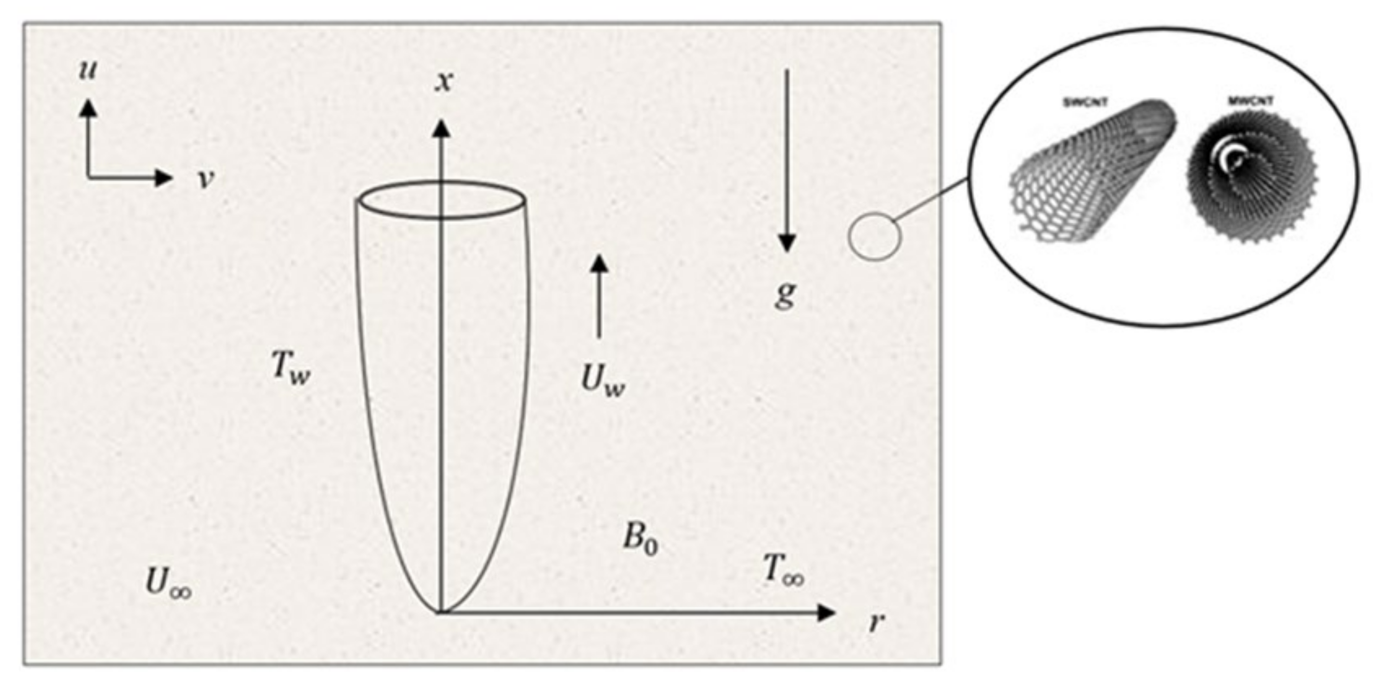
2. Problem Formation

An incompressible laminar of two-dimensional steady boundary layer with a combination of SWCNT and MWCNT hybrid nanofluid passing through a moving vertical slander needle was used. The needle was considered slender if the thickness of the needle did not exceed that of the boundary layer above it. Figure 1 shows the schematic representation of the physical model and coordinate system where x and r are the axial and radial coordinates, respectively, in which the radius is given by $r=R\left(x\right)$. The x-axis measures the leading edge of the needle in the vertical direction, while r is always normal to the x-axis. In this system, we assumed the temperature of needle surface is $T_w$ and the ambient temperature $T_{\infty }$ where when $T_w>T_{\infty }$ corresponds to a heated needle (assisting flow) and when $T_w<T_{\infty }$ corresponds to a cooled needle (opposing flow). Meanwhile, the needle moves with a constant velocity, $U_w$, in the same or opposite way to the free stream velocity, $U_{\infty }$. The magnetic field, $B_0$, is imposed parallel to the direction of the flow. Since the needle is assumed slender, the pressure gradient along the body is neglected but the importance is on the effect of its transverse curvature [45].

Using the above assumption, the governing equations for continuity, momentum, and energy for this problem are written in the cylindrical coordinates of x and r as follows [34,46]:

$$\frac{\partial }{\partial x}\left(ru\right)+\frac{\partial }{\partial r}\left(r\upsilon \right)=0$$

(1)

$$u\frac{\partial u}{\partial x}+\upsilon \frac{\partial u}{\partial r}=\frac{{\mu }_{hnf}}{{\rho }_{hnf}}\left(\frac{1}{r}\right)\frac{\partial }{\partial r}\left(r\frac{\partial u}{\partial r}\right)-\frac{{\sigma }_{hnf}{B}^2}{{\rho }_{hnf}}u+\frac{g{\left(\rho \beta \right)}_{hnf}}{{\rho }_{hnf}}\left(T-T_{\infty }\right)$$

(2)

$$u\frac{\partial T}{\partial x}+\upsilon \frac{\partial T}{\partial r}={\alpha }_{hnf}\left(\frac{1}{r}\right)\frac{\partial }{\partial r}\left(r\frac{\partial T}{\partial r}\right)$$

(3)

with boundary conditions (BCs)

$$\begin{gathered} u=U_w, \upsilon =0, T=T_w=T_{\infty }+T_0{\left(x/L\right)}^2 \mathrm{at} r=R\left(x\right); \\ u\to U_{\infty }, T\to T_{\infty } \mathrm{at} r\to \infty \end{gathered}$$

(4)

in which u and $\upsilon$ are the component of velocity for x axes and r axes, respectively ${\alpha }_{hnf}=k_{hnf}/{\left(\rho c_p\right)}_{hnf}$ is the thermal diffusivity of the hybrid nanofluid. Meanwhile, $g$ is the gravity acceleration and $B=\sqrt{2B_0/x}$ refers to the magnetic field applied to the fluid flow. The induced magnetic field was disregarded since the magnetic number of Reynolds, R_m, is assumed to be very small. The hybrid nanofluid’s thermophysical attributes are described in

Table 1. Base fluid and nanoparticle numerical values for thermophysical properties [47].

Thermophysical Properties	k (W/mK)	Cp (J/kgK)	ρ (kg/m3)	β × 10−6 (1/K)
SWCNT	6600	425	2600	19
MWCNT	3000	796	1600	21
Water	0.613	4179	997	210

.

Following [48,49], a set of thermophysical properties that relate to these parameters are simplified in

Table 2. Hybrid nanofluid’s thermophysical properties [48,49].

Thermophysical	Hybrid Nanofluids
Density	${\rho }_{hnf}=\left(1-{\phi }_2\right)\left[\left(1-{\phi }_1\right){\rho }_f+{\phi }_1{\rho }_{s1}\right]+{\phi }_2{\rho }_{s2}$
Heat Capacity	${\left(\rho C_p\right)}_{hnf}=\left(1-{\phi }_2\right)\left[\left(1-{\phi }_1\right){\left(\rho C_p\right)}_f+{\phi }_1{\left(\rho C_p\right)}_{s1}\right]+{\phi }_2{\left(\rho C_p\right)}_{s2}$
Viscosity	${\mu }_{hnf}=\frac{{\mu }_f}{{(1-{\phi }_1)}^{2.5}{(1-{\phi }_2)}^{2.5}}$
Thermal Conductivity	$k_{hnf}=\left[\frac{1-{\phi }_2+2{\phi }_2\left(\frac{k_S}{k_S-k_{nf}}\right)\mathit{ln}\left(\frac{k_S+k_{nf}}{2k_{nf}}\right)}{1-{\phi }_2+2{\phi }_2\left(\frac{k_{nf}}{k_S-k_{nf}}\right)\mathit{ln}\left(\frac{k_S+k_{nf}}{2k_{nf}}\right)}\right]k_{nf}$ $k_{nf}=\left[\frac{k_{s1}+2k_f-2{\phi }_1\left(k_f-k_{s1}\right)}{k_{s1}+2k_f+{\phi }_1\left(k_f-k_{s1}\right)}\right]k_f$
Thermal Expansion Coefficient	${\left(\rho \beta \right)}_{hnf}=\left(1-{\phi }_2\right)\left[\left(1-{\phi }_1\right){\left(\rho \beta \right)}_f+{\phi }_1{\left(\rho \beta \right)}_{s1}\right]+{\phi }_2{\left(\rho \beta \right)}_{s2}$

. The formation of hybrid nanofluid was formed by mixing the MWCNT nanoparticles into 0.01 volume of SWCNT/water. It is worth highlighting that 0.01 volume of solid fraction SWCNT $\left({\phi }_1=0.01\right)$ was added constantly to the water throughout most of the problem. Meanwhile, to produce a SWCNT-MWCNT/water, various volumes of solid fraction of MWCNT $\left({\phi }_2\right)$ were added.

The subscripts of hnf, nf, and f representi the three categories of fluids, which are hybrid nanofluids, nanofluids, and fluids, respectively. While, ${\phi }_1$ and ${\phi }_2$ for two different nanoparticles of solid volume fractions which ${\phi }_1$ is for SWCNT and ${\phi }_2$ is for MWCNT. Besides, s1 was definitely for SWCNT s2 for MWCNT nanoparticles and $S=s1+s2$.

To solve the governing equations, similarity resolution was acquired to diminish the independent variable of x and r. Thus, the above partial differential equations were reduced into ordinary differential equations with η as the new independent variable. Introducing a stream function, $\psi$, where $u=\frac{1}{r}\frac{\partial \psi }{\partial r}$ and $\upsilon =-\frac{1}{r}\frac{\partial \psi }{\partial x}$, the composite velocity between the needle and the free stream flow was define as $U=U_w+U_{\infty }$. Hence, the obtaining similarities are:

$$\eta =U{r}^2/{\nu }_{f}x, \psi ={\nu }_{f}xf\left(\eta \right), T=\left(T_w-T_{\infty }\right)\theta \left(\eta \right)+T_{\infty }, {\nu }_f=\frac{{\mu }_f}{{\rho }_f}$$

(5)

Thus, Equation (1) was satisfied identically. Equation (6) signifies the size of the needle where

$$R\left(x\right)={\left({\mathsf{\nu }}_{f}cx/U\right)}^{\frac{1}{2}}$$

(6)

Invoke Equation (5) into Equations (2) and (3), and set $c=\eta$, the reduction of momentum and energy equations are in the following form:

$$2\frac{{\mu }_{hnf}/{\mu }_f}{{\rho }_{hnf}/{\rho }_f}\left(\eta f^{‴}+f^{″}\right)+f{f}^{″}-M{f}^{\prime }+\frac{{\left(\rho \beta \right)}_{hnf}/{\left(\rho \beta \right)}_f}{{\rho }_{hnf}/{\rho }_f}\frac{\lambda }{4}\theta =0$$

(7)

$$\frac{2}{Pr}\frac{k_{hnf}/k_f}{{\left(\rho C_p\right)}_{hnf}/{\left(\rho C_p\right)}_f}\left(\eta {\theta }^{″}+{\theta }^{\prime }\right)+f{\theta }^{\prime }-2f^{\prime }\theta =0$$

(8)

along the BCs,

$$\begin{array}{c}\hfill f\left(c\right)=\frac{1}{2}\epsilon c, f^{\prime }\left(c\right)=\frac{1}{2}\epsilon , \theta \left(c\right)=1\hfill \\ f^{\prime }\left(\infty \right)\to \frac{1-\epsilon }{2}, \theta \left(\infty \right)\to 0\hfill \end{array}$$

(9)

where $\lambda =G{r}_x/R{e}_x^2$ is the constant mixed convection parameter or Richardson number with $\lambda >0, \lambda =0$ and $\lambda <0$ represent the assisting flow, forced convection flow, and opposing flow, respectively. In this context, $G{r}_x=g{\beta }_f\left(T_w-T_{\infty }\right)x^3/{\nu }_f^2$ is the local Grashof number and $R{e}_x=Ux/{\nu }_f$ is the local Reynolds number. While $\epsilon =\frac{U_w}{U}$ is velocity ratio parameter between the needle and the free stream. Furthermore, parameter $M=\sigma B_0/{\rho }_{hnf}U$ is the magnetic field and $\mathit{Pr}=\frac{{\nu }_f}{{\alpha }_f}$ is a Prandtl number. Our interests in physical quantities are the skin friction coefficient, C_f, and local Nusselt number, Nu_x, which can be easily expressed as

$$C_f=\frac{{\mu }_{hnf}}{{\rho }_f{U}^2}{\left(\frac{\partial u}{\partial r}\right)}_{r=c},N{u}_x=-\frac{x{k}_{hnf}}{k_f\left(T_w-T_{\infty }\right)}{\left(\frac{\partial T}{\partial r}\right)}_{r=c}$$

(10)

Using Equations (5) and (6) to solve Equation (10), we have

$$C_f{({\mathit{Re}}_x)}^{\frac{1}{2}}=4\left({\mu }_{hnf}/{\mu }_f\right)c^{\frac{1}{2}}{f}^{″}\left(c\right), N{u}_x{({\mathit{Re}}_x)}^{-\frac{1}{2}}=-2\left(k_{hnf}/k_f\right)c^{\frac{1}{2}}{\theta }^{\prime }\left(c\right)$$

(11)

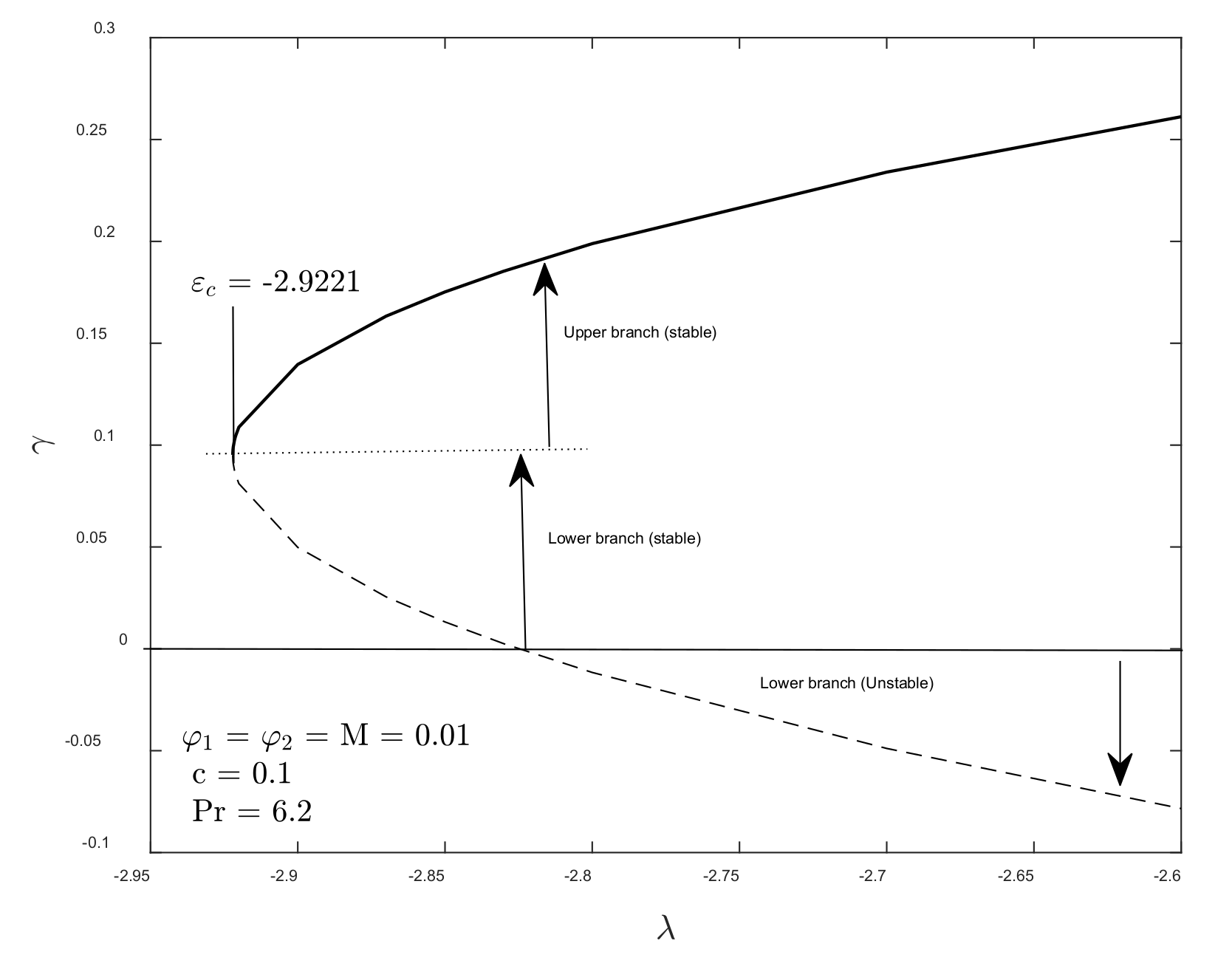
3. Stability Flow Solution

Ref. [50] conveyed the solution for stability analysis in his work. To test the fact that the two solutions are either stable or unstable, a stability analysis has to be conducted. Consider the unsteady form by adding $\frac{\partial u}{\partial t}$ and $\frac{\partial T}{\partial t}$ at the beginning of Equations (2) and (3), respectively, where t denotes the dimensionless time. Thus, we have

$$\frac{\partial u}{\partial t}+u\frac{\partial u}{\partial x}+\upsilon \frac{\partial u}{\partial r}=\frac{{\mu }_{hnf}}{{\rho }_{hnf}}\left(\frac{1}{r}\right)\frac{\partial }{\partial r}\left(r\frac{\partial u}{\partial r}\right)-\frac{\sigma B^2}{{\rho }_{hnf}}u+\frac{g{\left(\rho \beta \right)}_{hnf}}{{\rho }_{hnf}}\left(T-T_{\infty }\right)$$

(12)

$$\frac{\partial T}{\partial t}+u\frac{\partial T}{\partial x}+\upsilon \frac{\partial T}{\partial r}={\alpha }_{hnf}\left(\frac{1}{r}\right)\frac{\partial }{\partial r}\left(r\frac{\partial T}{\partial r}\right)$$

(13)

And the new similarity transformations are in the following form;

$$\eta =U{r}^2/{\nu }_{f}x, \psi ={\nu }_{f}xf\left(\eta ,\tau \right), T=\left(T_w-T_{\infty }\right)\theta \left(\eta ,\tau \right)+T_{\infty }, \tau =\frac{2Ut}{x}$$

(14)

Note that a new dimensionless similarity variable, $\tau =\frac{2Ut}{x}$, is introduced in order to model the problem for temporal stability analysis. It is worth addressing that the use of τ in relation to the initial value problem consistent with the solution that will be obtained in practice (stable and physically realizable). Apply Equation (14) into Equation (12) and Equation (13), we have

$$2\frac{{\mu }_{hnf}/{\mu }_f}{{\rho }_{hnf}/{\rho }_f}\left(\eta \frac{{\partial }^{3}f}{\partial {\eta }^3}+\frac{{\partial }^{2}f}{\partial {\eta }^2}\right)+\tau \left(\frac{\partial f}{\partial \eta }\frac{{\partial }^{2}f}{\partial \eta \partial \tau }-\frac{\partial f}{\partial \tau }\frac{{\partial }^{2}f}{\partial {\eta }^2}\right)-\frac{{\partial }^{2}f}{\partial \eta \partial \tau }+f\left(\eta ,\tau \right)\frac{{\partial }^{2}f}{\partial {\eta }^2}-M\frac{\partial f}{\partial \eta }+\frac{{\left(\rho \beta \right)}_{hnf}/{\left(\rho \beta \right)}_f}{{\rho }_{hnf}/{\rho }_f}\frac{\lambda }{4}\theta =0$$

(15)

$$\frac{2}{Pr}\frac{k_{hnf}/k_f}{{\left(\rho C_p\right)}_{hnf}/{\left(\rho C_p\right)}_f}\left(\eta \frac{{\partial }^2\theta }{\partial {\eta }^2}+\frac{\partial \theta }{\partial \eta }\right)+\tau \left(\frac{\partial f}{\partial \eta }\frac{\partial \theta }{\partial \tau }-\frac{\partial f}{\partial \tau }\frac{\partial \theta }{\partial \eta }\right)-2\theta \frac{\partial f}{\partial \eta }-\frac{\partial \theta }{\partial \tau }+f\left(\eta ,\tau \right)\frac{\partial \theta }{\partial \eta }=0$$

(16)

subjected to BCs,

$$\begin{array}{c}\hfill f\left(c,\tau \right)=\frac{1}{2}\epsilon c, \frac{\partial f}{\partial \eta }\left(c,\tau \right)=\frac{1}{2}\epsilon , \theta \left(c,\tau \right)=1\hfill \\ \frac{\partial f}{\partial \eta }\left(\infty ,\tau \right)\to \frac{1-\epsilon }{2}, \theta \left(\infty ,\tau \right)\to 0\hfill \end{array}$$

(17)

To determine the stability of the steady flow solution $f\left(\eta \right)=f_0\left(\eta \right) \mathrm{and} \theta \left(\eta \right)={\theta }_0\left(\eta \right)$ that satisfied Equations (7) and (8), we introduced these linearized eigenvalues equations such as in [51]:

$$\begin{gathered} f\left(\eta ,\tau \right)=f_0\left(\eta \right)+e^{-\gamma \tau }F\left(\eta ,\tau \right) \\ \theta \left(\eta ,\tau \right)={\theta }_0\left(\eta \right)+e^{-\gamma \tau }G\left(\eta ,\tau \right) \end{gathered}$$

(18)

where $F\left(\eta ,\tau \right) \mathrm{and} G\left(\eta ,\tau \right)$ are set as the small relative to $f_0\left(\eta \right)$ and ${\theta }_0\left(\eta \right)$ respectively while $\gamma$ is an unknown parameter of eigenvalue. In order to identify the growth or decomposition of Equation (18), we need to set $\tau =0 ,$ so that the function of $F$ and $G$ can be written as $F_0$ and $G_0$. Differentiating Equation (18) and equating it to Equations (15) and (16), we obtain the following linearized eigenvalue equations:

$$2\frac{{\mu }_{hnf}/{\mu }_f}{{\rho }_{hnf}/{\rho }_f}\left(\eta F_0{}^{‴}+F_0{}^{″}\right)+f_0{}^{″}{F}_0+\gamma F_0{}^{\prime }+f_0{F}_0{}^{″}-M{F}_0{}^{\prime }+\frac{{\left(\rho \beta \right)}_{hnf}/{\left(\rho \beta \right)}_f}{{\rho }_{hnf}/{\rho }_f}\frac{\lambda }{4}{G}_0=0$$

(19)

$$\frac{2}{Pr}\frac{k_{hnf}/k_f}{{\left(\rho C_p\right)}_{hnf}/{\left(\rho C_p\right)}_f}\left(\eta G_0{}^{″}+G_0{}^{\prime }\right)+\gamma G_0+f_0{G}_0{}^{\prime }+F_0{\theta }_0{}^{\prime }=0$$

(20)

with BCs;

$$\begin{array}{c}\hfill F_0{}^{\prime }\left(c\right)=0, F_0\left(c\right)=0, G_0\left(c\right)=0\hfill \\ F_0{}^{\prime }\left(\infty \right)\to 0, G_0\left(\infty \right)\to 0\hfill \end{array}$$

(21)

After the meticulous derivation of Equations (19)–(21), the stability of the corresponding steady flow solution of $f_0$ and $G_0$ was determined by the least eigenvalue $\gamma$. According to [52], after relaxation of the BC on $F_0{}^{\prime }\left(\eta \right) \mathrm{or} G_0\left(\eta \right)$, the range of possible eigenvalues can be resolute. In this problem, $F_0{}^{\prime }\left(\infty \right)\to 0$ was chosen to be relaxed and a new boundary condition was presented, which is $F_0{}^{″}\left(0\right)=1$, in order to replace the relaxing condition. Results on stability were obtained using bvp4c MATLAB.

4. Numerical Computation

There is a lot of computational programming to solve the boundary layer problem. Some researchers are familiar with MAPLE, Fortran, or MATLAB. However, generally, researchers would like to use a higher-order method that is robust and capable of solving systems of equations. So, bvp4c in MATLAB was chosen because it offers a convenient and proficient in solving fairly sophisticated problems, especially for solving nonlinear systems of equations [53,54]. The algorithm relies on an iteration structure. BVP4C is, in particular, a coding that implements the Lobatto IIIa three-stage formula. This is a collocation formula which is formed by a polynomial collocation. It provides a C¹-continuous solution that is fourth-order accurate uniformly in x ∈ [a, b]. The crucial part in solving the bvp4c is the variation step and early guessing of the mesh point. Besides, the efficiency will eventually depend on one’s ability to provide the algorithm with an initial guess for the solution. We created two folders, namely, code a and code b, for the trial-and-error initial guess and continuous iterations that nearly to the initial guess, respectively. To initiate the computation, the reduction of Equations (7) and (8) together with the BCs (9) to a set of first order is essential. Let,

$$f=y\left(1\right), f^{\prime }=y\left(2\right),f^{″}=y\left(3\right),f^{‴}=\frac{1}{\eta }\left[\frac{-y\left(1\right)y\left(3\right)+My\left(2\right)-\frac{J\lambda }{B4}y\left(4\right)}{2\left(\frac{{\mu }_{hnf}/{\mu }_f}{{\rho }_{hnf}/{\rho }_f}\right)}-y\left(3\right)\right]$$

(22)

and

$$\theta =y\left(4\right),{\theta }^{\prime }=y\left(5\right), {\theta }^{″}=\frac{1}{\eta }\left[\frac{-Pr\left(2y\left(2\right)y\left(4\right)-y\left(1\right)y\left(5\right)\right)}{2\left(\frac{k_{hnf}/k_f}{{\left(\rho C_p\right)}_{hnf}/{\left(\rho C_p\right)}_f}\right)}-y\left(5\right)\right]$$

(23)

The BCs in Equation (9) become,

$$\begin{array}{c}\hfill ya\left(1\right)=\epsilon c/2, ya\left(2\right)=\epsilon /2, ya\left(4\right)=1\hfill \\ yb\left(2\right)\to \left(1-\epsilon \right)/2, yb\left(4\right)\to 0\hfill \end{array}$$

(24)

Some commands in handling the function such as @odeBVP and @odeBC are from the syntax of the solver sol = bvp4c (@OdeBVP, @OdeBC, solinit, options). These commands are specified by Equations (22) and (23) and boundary conditions of Equation (24). The numerical results obtained from the solver are transformed to graphs. Duality solutions exist to the problem and also satisfy the boundary conditions. Further information regarding on bvp4c can be found in [55].

5. Analysis of Result

The numerical computations were carried out for several values of considered parameters which are M, $\lambda$, $c, \phi$, and $\epsilon$ in order to furnish a clear understanding to the problem. The range of values of the parameters are $M\left(0\le M\le 0.05\right)$, $c\left(0.1\le c\le 0.2\right)$, and ${\phi }_1\left(0\le {\phi }_1\le 0.03\right)$ and the fixed values of $Pr=6.2$. Equations (7) and (8) along the BCs (9) were computed numerically using bvp4c in MATLAB. The bvp4c solver uses the finite difference method. It requires a person to set an initial guess supplied at the initial mesh point and changing the step size in order to obtain the specified accuracy.

Table 3. Comparison values of $f^{″}\left(c\right)$ when $M=\lambda =\epsilon ={\phi }_1={\phi }_2=0$ for some thicknesses of needles, $c$ when $Pr=1$.

c	[56]	[57]	Present Study
0.01	8.492436	8.4924453	8.4924451
0.1	1.2888171	1.2888300	1.2888300
0.15		0.9383388	0.9383388

outlines the data produced by the present code and those reported by [56,57] when $M=\lambda =\epsilon ={\phi }_1={\phi }_2=0$. It shows a great agreement, and hence we are confident to present our results.

Figure 2 portrays the result for three types of fluid, which are viscous fluid $\left({\phi }_1={\phi }_2=0\right),$ SWCNT/water $\left({\phi }_1=0.01,{\phi }_2=0\right),$ MWCNT/water $\left({\phi }_1=0,{\phi }_2=0.010\right),$ and SWCNT-MWCNT/water $\left({\phi }_1=0.01,{\phi }_2=0.01\right)$ on variation of shear stress, $f^{″}\left(c\right),$ and local heat flux, $-{\theta }^{\prime }\left(c\right)$. As we observed, we can see that hybrid nanofluid was highest compared with the viscous fluid and nanofluids in $f^{″}\left(c\right)$ and $-{\theta }^{\prime }\left(c\right)$. Furthermore, we noticed that hybrid nanofluid delayed the separation of the boundary layer. Besides, the dual solutions seemed to exist at $\epsilon <0$, where the flow moves in opposite directions. In summary, the range of the dual solution was at ${\epsilon }_c<\epsilon \le -1.5$ while no solution was found at $\epsilon <{\epsilon }_c$.

The result on the influence of size needle, $c$ on the variation of shear stress, $f^{″}\left(c\right)$ and local heat flux, $-{\theta }^{\prime }\left(c\right)$ is plotted in Figure 3. It can be seen that the shear stress for $c=0.1$ was higher compared to $c=0.2$. This is because the interaction between the needle surface and the fluid particles decreases when the size of needle decreases, which leads to the reduction of the drag force. Furthermore, the decreasing size of the needle gives a high thermal conductivity, allowing the heat being conducted from the surface through the needle to increase. It is also noted that the range of the solution widens as $c$ increases, hence shortening the separation of the boundary layer. In particular, the dual solutions exist when ${\epsilon }_c<\epsilon \le -2$ for both $c=0.1$ and $c=0.2$, respectively.

Variation shear stress, $f^{″}\left(c\right)$, and local heat flux, $-{\theta }^{\prime }\left(c\right)$, with mixed convection parameter, $\lambda$, for different values of M are presented in Figure 4. It is noticed that the values of $f^{″}\left(c\right)$ and $-{\theta }^{\prime }\left(c\right)$ decrease when the imposed M is larger, following the fact that the rising strength of M will offer larger resistance on the fluid particles and cause the heat to be generated in the fluid. Therefore, a drag force known as Lorentz force is formed. This force may oppose and decelerate the motion of the hybrid nanofluid consequently, and reduce the wall friction and temperature, respectively. Besides, the stronger M makes the boundary layer become skinny and also reduces the range of boundary layer separation. Meaning, the boundary layer separation becomes faster as the value of M increases. It can be seen that the critical values of $\lambda$, ${\lambda }_c$ increase, i.e., $M=0\left( {\lambda }_c=-3.1051\right),$ $M=0.01\left( {\lambda }_c=-2.9221\right),$ and $M=0.05\left( {\lambda }_c=-2.2850\right).$ Duality of solutions exist when ${\lambda }_c<\lambda \le 0,$ a unique solution appears at $\lambda >0$, and no solution was found at $\lambda <{\lambda }_c$. The buoyance force effect can be seen in assisting flow $\lambda >0$ if the Prandtl number is set lower. According to [58], the physical explanation behind this is that the effect of buoyancy force is higher in low Prandtl number fluid. Due to the low fluid viscosity, the velocity in the boundary layer increases as the assisting buoyancy force functions as a favorable pressure gradient. For opposing flow $(\lambda <0$), the buoyancy force is contrary to fluid movement, and hence the fluid is delayed, thus reducing the magnitude of velocity profiles within the boundary layer significantly. Thus, a reverse flow happens for $\lambda =-1$ near the surface. On the other note, the effect of $\lambda$ is relatively less in $-{\theta }^{\prime }\left(c\right)$ because $\lambda$ does not appear in Equation (8).

Quite interesting result is on variation of shear stress, $f^{″}\left(c\right)$, and local heat flux, $-{\theta }^{\prime }\left(c\right)$, with $\lambda$ for different values of ${\phi }_1$. It is observed from Figure 5 that the increasing of ${\phi }_1$ increased the $f^{″}\left(c\right)$ near the wall and $-{\theta }^{\prime }\left(c\right)$ on the surface. The results showed good agreement with the experimental studies conducted by [59,60]. Increasing of volume fractions nanoparticles led to the increasing of the surface tension of the hybrid nanofluid. The number of nanoparticles suspended in the base fluid increased, which moved more nanoparticles to the liquid surface and adjacent to each other. As a result, an attractive force called Van der Waals forces occurred between the molecules, resulting in higher surface tension and consequently increased the shear stress. The strong force exerted between molecules led to the higher $-{\theta }^{\prime }\left(c\right)$. Duality of the solution exists at the opposing flow $\lambda <0,$ between the range ${\lambda }_c<\lambda \le -1,$ a unique solution appears at $\lambda >0$, and no solution was found at $\lambda <{\lambda }_c$. Besides, it can be seen clearly from the graph that the critical value, ${\lambda }_c$, decreased as ${\phi }_1$ increased, such as ${\phi }_1=0 \left({\lambda }_c=-2.8431\right)$, ${\phi }_1=0.01 \left({\lambda }_c=-2.9221\right)$, and ${\phi }_1=0.03 \left({\lambda }_c=-3.0880\right)$.

Next, Figure 6 shows the influence of ${\phi }_2$ on variation of $C_f$ and $N{u}_x$. Increasing ${\phi }_2$ will consequently increase $C_f$ as ${\phi }_1$ increases. Viscosity rate changes were barely observed at low fractions, likewise at high volume fractions. This is because the deposited of nanoparticles molecules increased the flow resistance, which resulted in increasing the shear stress and heat transfer.

The behavior of $C_f$ and $N{u}_x$ with $\phi$ for different values of c is depicted in Figure 7. It can be observed that $C_f$ and $N{u}_x$ accelerated upwards with the increase of c as the value of $\phi$ increased. Note that both graphs are affected by the variation of c, as we can see in Equation (11). The friction force on the needle surface and fluid flow enhances due to the interaction between the needle’s surface area and fluid particles when the size of the needle becomes bigger. The $N{u}_x$ for $c=0.2$ is higher compared with when $c=0.1$. This follows the fact that heat transfer increases as the needle diameter increases because a large surface area requires higher temperature.

Figure 8 shows the influence of M on variation of $C_f$ and $N{u}_x$ with $\phi$. Both graphs portray that the value of $C_f$ and $N{u}_x$ decreases with the increase in M and also increase with higher values of $\phi$. It can be envisioned from the graph that the flow is flowing far from the surface instead of it became nearer to the surface when M is prominent. The reason for this behavior is because of the stronger interaction between the nanoparticles as $\phi$ increase but the motion was retarded by the Lorentz force that will gives disturbance to the flow. Thus, enhancing M tends to decrease both of $C_f$ and $N{u}_x$.

Figure 9, Figure 10 and Figure 11 illustrate the variation of the velocity and temperature profiles for several parameters such as $M, c$ and ${\phi }_2$. We realized that the duality of solutions which happened in $f\prime \left(\eta \right)$ and $\theta \left(\eta \right)$ supported the duality obtained from Figure 2, Figure 3, Figure 4 and Figure 5 in this study. Figure 9 depicts the effect of $M$ on both $f\prime \left(\eta \right)$ and $\theta \left(\eta \right)$. It can be observed that the Lorenz force retard the motion of the fluid, which decreased the velocity as $M$ increased, but opposite trait happened on $\theta \left(\eta \right)$, where the force generated and consequently increased the heat as the value of $M$ increased. However, Figure 10 clearly shows that the increasing of $c$ slowed down the velocity but augmented the temperature of hybrid nanofluid for both branches. Furthermore, the effects of ${\phi }_2$ on $f\prime \left(\eta \right)$ and $\theta \left(\eta \right)$ can be seen in Figure 11. In addition, all these profiles addressed and fulfilled the endpoint of BCs Equation (8) asymptotically.

The duality solutions obviously occurred at most in our numerical graph. Due to that, a stability analysis has to be conducted to test which explanations lead to a stable and reliable solution. To initiate them, we applied Equations (19)–(21) along with the new boundary condition into bvp4c in MATLAB software. In defining stability of the two solutions, the $\gamma$ value is important. Numerical values obtained are written in

Table 4. Least eigenvalues $\gamma$ for selected ${\phi }_2$ with several values of M when ${\phi }_2=0.01$, $\epsilon =-0.3$ and $c=0.1$.

${\displaystyle {\mathit{\phi }}_{\mathbf{1}}}$	M	λ	First Solution	Second Solution
	0	−3.1048	0.0987	0.0804
		−3.104	0.1038	0.0800
		−3.09	0.1156	0.0792
	0.01	−2.9219	0.0991	0.0908
0.01		−2.921	0.1049	0.0850
		−2.92	0.1088	0.0811
	0.05	−2.2848	0.1037	0.0942
		−2.284	0.1088	0.0891
		−2.28	0.1205	0.0773
	0	−3.2781	0.1004	0.0918
		−3.278	0.1013	0.0909
		−3.27	0.1229	0.7946
	0.01	−3.0878	0.1009	0.0796
0.03		−3.087	0.1061	0.0792
		−3.08	0.1170	0.0780
	0.05	−2.4245	0.1050	0.0971
		−2.424	0.1088	0.0933
		−2.42	0.1213	0.0807

and

Table 5. Least eigenvalues $\gamma$ $c$ when ${\phi }_1={\phi }_2=0.01$ and $\lambda =-0.2$.

c	M	ε	First Solution	Second Solution
	0	−3.1121	0.1884	0.1356
		−3.112	0.1954	0.1673
		−3.11	0.2085	0.1903
	0.01	−2.9895	0.2443	0.1311
0.1		−2.989	0.2515	0.1019
		−2.98	0.2651	0.0871
	0.05	−2.5829	0.2011	0.1105
		−2.582	0.2205	0.1041
		−2.58	0.2240	0.1004
	0	−2.5010	0.1720	0.0983
		−2.495	0.1902	0.0796
		−2.49	0.2015	0.0679
	0.01	−2.4265	0.2005	−0.2011
0.2		−2.426	0.2104	−0.2201
		−2.42	0.2511	−0.2220
	0.05	2.1011	0.1372	0.1013
		−2.101	0.1518	0.0987
		−2.10	0.1729	0.0857

. Clearly, we can see that the first solution yielded a positive value of $\gamma$ which is similar with the aforesaid [61,62,63]. However, an intriguing pattern was noticed at the second solution, where we also obtained positive values of $\gamma$ for several $\lambda \to {\lambda }_c$. Figure 12 illustrates that for negative values of $\gamma$, the second solution specifies as an unstable solution; likewise for the positive value of $\gamma$, the second solution signifies as a stable solution. The explanation behind this is due to the rapid transition from turbulence flow to laminar flow. Generally, the boundary layer thickness for second solution is always thicker compared with the first solution. In this case, it is assumed that the laminar flow takes place in the thin boundary layer while the turbulence flow occurs in the thick boundary. For the present problem, the formation of the boundary layer was complicated with the presence of M, which gave an advantage for the turbulent flow to exchange to laminar flow.

6. Conclusions

This study was on mixed convection over a vertical moving slender needle which took into account the effect of M, c, $\lambda$ and thermophysical properties (${\phi }_1$ and ${\phi }_2$) on velocity, temperature, skin friction, and local Nusselt number. Therefore, the findings can be summarized in three important parts:

• Duality Solution
  • The presence of the duality solutions is prominent when in opposing flow $\lambda <0$
  • The range of duality of solutions is widely expanded under the influence of smaller $M$ and $c$
  • Hybrid nanofluid possess faster boundary layer separation compared with viscous fluid and nanofluid.
  • The increment of c shortens the connection of first and second solution.
  • Stability analysis shows that first solution is favorable compared with the second solution.
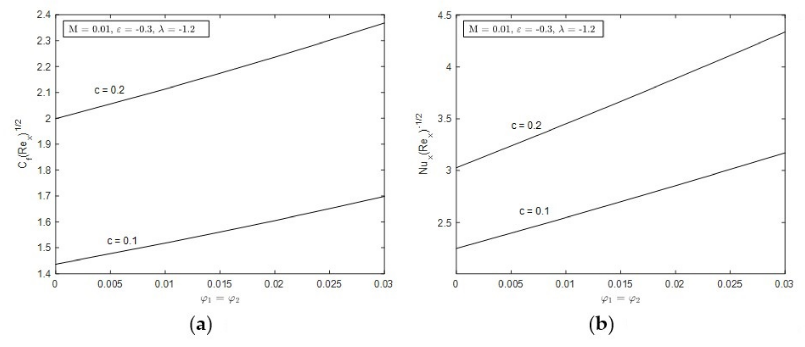
• Skin Friction
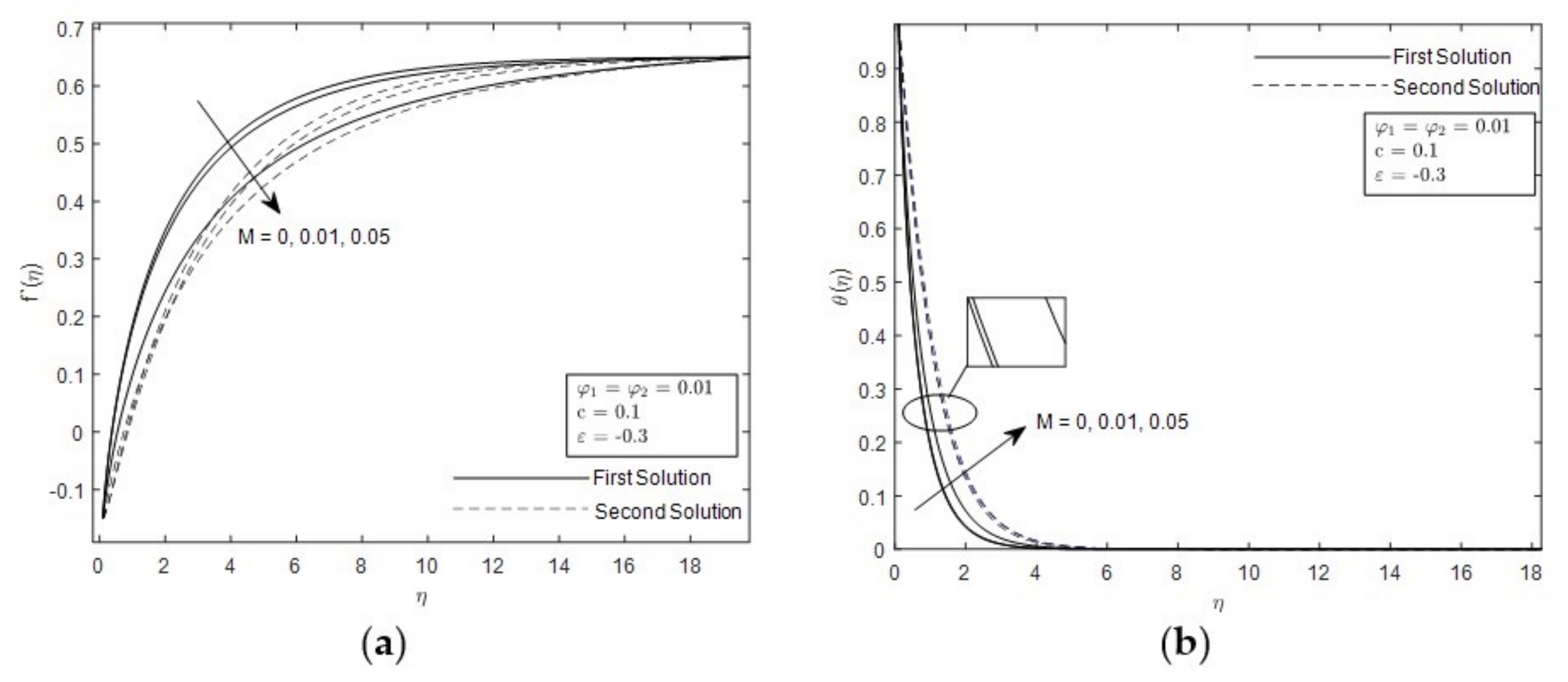
  • Hybrid nanofluid reduced the value of skin friction as the value of M increased.
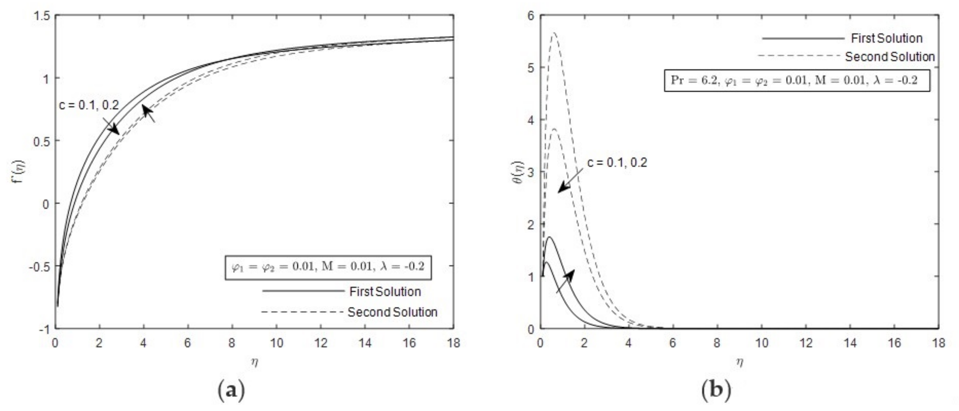
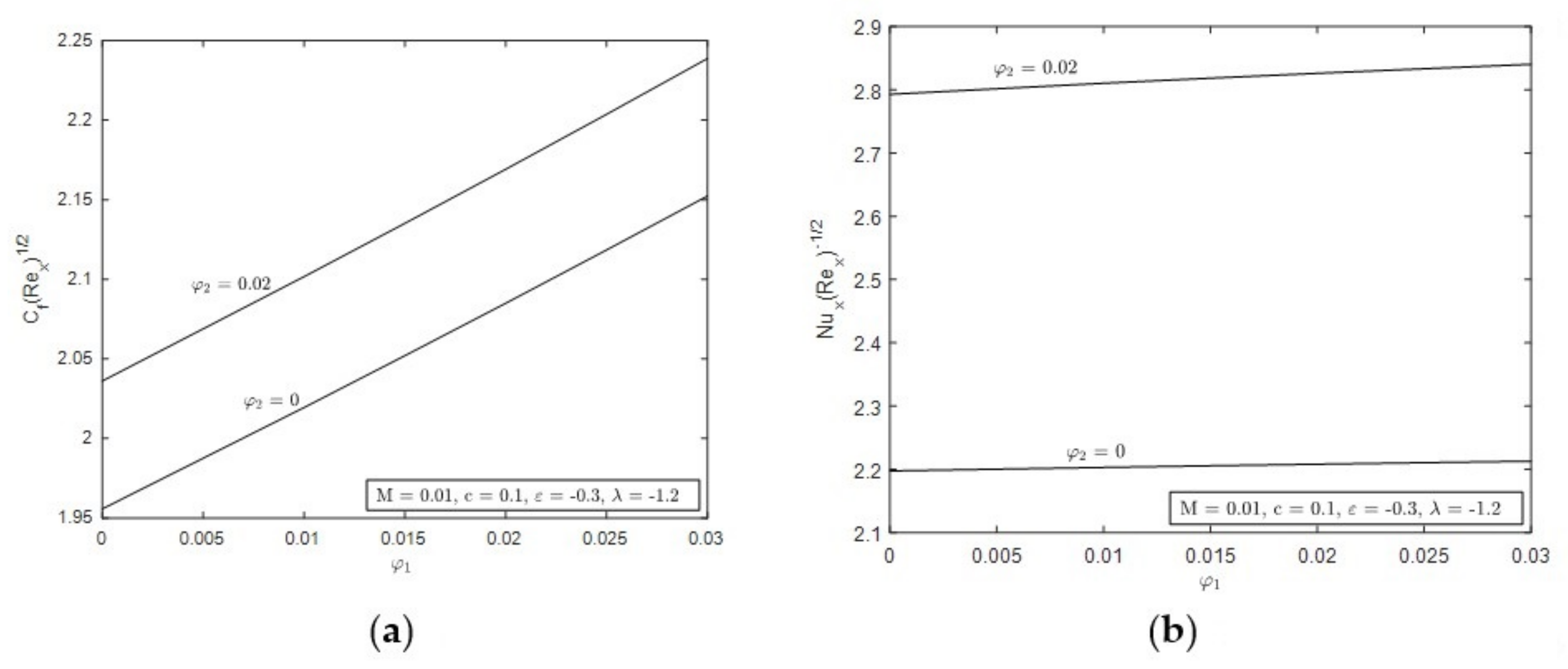
  • Hybrid nanofluid enhanced the skin friction as the concentration of the nanoparticles and c increased.
• Heat Transfer
  • Hybrid nanofluid reduced the value of heat transfer as the value of M increased.
  • Hybrid nanofluid enhanced the heat transfer as the concentration of the nanoparticles and c increased.

References

1. Choi, S.U.; Eastman, J.A. Enhancing Thermal Conductivity of Fluids with Nanoparticles; No. ANL/MSD/CP-84938; CONF-951135-29; Argonne National Lab.: Lemont, IL, USA, 1995.
2. Rao, Y. Nanofluids: Stability, phase diagram, rheology and applications. Particuology 2010, 8, 549–555. [Google Scholar] [CrossRef]
3. Lim, A.E.; Lam, Y.C. Numerical Investigation of Nanostructure Orientation on Electroosmotic Flow. Micromachines 2020, 11, 971. [Google Scholar] [CrossRef] [PubMed]
4. El-Aziz, M.A.; Aly, A.M. MHD Boundary Layer Flow of a Power-Law Nanofluid Containing Gyrotactic Microorganisms Over an Exponentially Stretching Surface. CMC-Comput. Mater. Contin. 2020, 62, 525–549. [Google Scholar] [CrossRef]
5. Ranga, B.J.A.; Kumar, K.K.; Rao, S.S. State-of-art review on hybrid nanofluids. Renew. Sustain. Energy Rev. 2017, 77, 551–565. [Google Scholar] [CrossRef]
6. Haq, R.U.; Raza, A.; Algehyne, E.A.; Tlili, I. Dual nature study of convective heat transfer of nanofluid flow over a shrinking surface in a porous medium. Int. Commun. Heat Mass Transf. 2020, 114, 104583. [Google Scholar] [CrossRef]
7. Xu, N.; Xu, H.A. A modified model for isothermal homogeneous and heterogeneous reactions in the boundary-layer flow of a nanofluid. Appl. Math. Mech.-Engl. Ed. 2020, 41, 479–490. [Google Scholar] [CrossRef]
8. Kudenatti, R.B.; Misbah, N.E.; Bharathi, M.C. Linear Stability of Momentum Boundary Layer Flow and Heat Transfer Over a Moving Wedge. ASME J. Heat Transf. 2020, 142, 061804. [Google Scholar] [CrossRef]
9. Ghalambaz, M.; Zadeh, S.M.H.; Mehryan, S.A.M.; Pop, I.; Wen, D. Analysis of melting behavior of PCMs in a cavity subject to a non-uniform magnetic field using a moving grid technique. Appl. Math. Model. 2020, 77, 1936–1953. [Google Scholar] [CrossRef]
10. Radushkevich, L.; Lukyanovich, V. O strukture ugleroda, obrazujucegosja pri termiceskom razlozenii okisi ugleroda na zeleznom kontakte. Zurn Fisic Chim 1952, 26, 88–95. [Google Scholar]
11. Iijima, S. Helical microtubules of graphitic carbon. Nature 1991, 354, 56. [Google Scholar] [CrossRef]
12. Iijima, S.; Ichihashi, T. Single-shell carbon nanotubes of 1-nm diameter. Nature 1993, 363, 603–605. [Google Scholar] [CrossRef]
13. Hayat, T.; Khursheed, M.; Farooq, M.; Alsaedi, A. Melting heat transfer in stagnation point flow of carbon nanotubes towards variable thickness surface. AIP Adv. 2016, 6, 015214. [Google Scholar] [CrossRef]
14. Shafiq, A.; Sindhu, T.N.; Al-Mdallal, Q.M. A sensitivity study on carbon nanotubes significance in Darcy–Forchheimer flow towards a rotating disk by response surface methodology. Sci. Rep. 2021, 11, 8812. [Google Scholar] [CrossRef] [PubMed]
15. Alawi, O.A.; Mallah, A.R.; Kazi, S.N.; Sidik, N.A.C.; Najafi, G. Thermophysical properties and stability of carbon nanostructures and metallic oxides nanofluids. J. Therm. Anal. Calorim. 2019, 135, 1545–1562. [Google Scholar] [CrossRef]
16. Acharya, N.; Bag, R.; Kundu, P.K. On the mixed convective carbon nanotube flow over a convectively heated curved surface. Heat Transf. 2020, 49, 1713–1735. [Google Scholar] [CrossRef]
17. Kamis, N.I.; Basir, M.F.M.; Jaafar, N.A.; Shafie, S.; Khairuddin, T.K.A.; Naganthran, K. Heat Transfer and Boundary Layer Flow Through A Thin Film of Hybrid Nanoparticles Embedded in Kerosene Base Fluid Past an Unsteady Stretching Sheet. Open J. Sci. Technol. 2020, 3, 322–334. [Google Scholar]
18. Olagunju, D.O. A self-similar solution forced convection boundary layer flow of a PENE-P fluid. Appl. Math. Lett. 2006, 19, 432–436. [Google Scholar] [CrossRef] [Green Version]
19. Munir, A.; Shahzad, A.; Khan, M. Forced convective heat transfer in boundary layer flow of Sisko fluid over a nonlinear stretching sheet. PLoS ONE 2014, 9, e100056. [Google Scholar] [CrossRef]
20. Sonawane, S.; Bhandarkar, U.; Puranik, B. Modeling Forced Convection Nanofluid Heat Transfer Using an Eulerian–Lagrangian Approach. ASME J. Therm. Sci. Eng. Appl. 2016, 8, 031001. [Google Scholar] [CrossRef]
21. Ma, Y.; Mohebbi, R.; Rashidi, M.M.; Yang, Z.; Fang, Y. Baffle and geometry effects on nanofluid forced convection over forward- and backward-facing steps channel by means of lattice Boltzmann method. Phys. A Stat. Mech. Its Appl. 2020, 554, 124696. [Google Scholar] [CrossRef]
22. Goodrich, S.S.; Marcum, W.R. Natural convection heat transfer and boundary layer transition for vertical heated cylinders. Exp. Therm. Fluid Sci. 2019, 105, 367–380. [Google Scholar] [CrossRef]
23. Saini, V.; Jauhri, S.; Gour, P.S. Study of boundary layer flow with natural convective boundary condition. Int. J. Innov. Res. Growth 2019, 8, 47–53. [Google Scholar] [CrossRef]
24. Zhao, Y.; Lei, C.; Patterson, J.C. Natural transition in natural convection boundary layers. Int. Commun. Heat Mass Transf. 2016, 76, 366–375. [Google Scholar] [CrossRef]
25. Fabregat, A.; Pallares, J. Heat transfer and boundary layer analyses of laminar and turbulent natural convection in a cubical cavity with differently heated opposed walls. Int. J. Heat Mass Transf. 2020, 151, 119409. [Google Scholar] [CrossRef]
26. Sparrow, E.M.; Eichhorn, R.; Gregg, J.L. Combined forced and free convection in a boundary layer flow. Phys. Fluids 1959, 2, 319–328. [Google Scholar] [CrossRef]
27. Aman, F.; Ishak, A. Mixed convection boundary layer flow towards a vertical plate with a convective surface boundary condition. Math. Probl. Eng. 2012, 2012, 453457. [Google Scholar] [CrossRef]
28. Galambaz, M.; Grosan, T.; Pop, I. Mixed convection boundary layer flow and heat transfer over a vertical embedded in a porous medium filled with suspension of nano-encapsulated phase change materials. J. Mol. Liq. 2019, 293, 111432. [Google Scholar] [CrossRef]
29. Maleque, K.A. Similarity requirements for mixed convective boundary layer flow over a vertical curvilinear porous surface with heat generation/absorption. Int. J. Aerosp. Eng. 2020, 2020, 7486971. [Google Scholar] [CrossRef] [Green Version]
30. Chen, J.L.S. Natural convection from needles with variable heat flux. J. Heat Transf. 1983, 105, 403–406. [Google Scholar] [CrossRef]
31. Chen, J.L.S. Mixed convection flow about slender bodies of revolution. J. Heat Transf. 1987, 109, 1033–1036. [Google Scholar] [CrossRef]
32. Wang, C.Y. Free convection plume from the tip of a vertical needle. Mech. Res. Commun. 1989, 16, 95–101. [Google Scholar] [CrossRef]
33. Ahmad, S.; Arifin, N.M.; Nazar, R.; Pop, I. Mixed convection boundary layer flow along vertical needles: Assisting and opposing flows. Int. Commun. Heat Mass Transf. 2008, 35, 157–162. [Google Scholar] [CrossRef]
34. Trimbitas, R.; Grosan, T. Mixed convection boundary layer flow along vertical thin needles in nanofluids. Int. J. Numer. Methods Heat Fluid Flow 2012, 24, 579–594. [Google Scholar] [CrossRef]
35. Salleh, S.N.A.; Bachok, N.; Arifin, N.M.; Ali, F.M.; Pop, I. Magnetohydrodynamics flow past a moving vertical thin needle in a nanofluid with stability analysis. Energies 2018, 11, 3297. [Google Scholar] [CrossRef] [Green Version]
36. Suresh, S.; Venkitaraj, K.P.; Slevakumar, P.; Chandrasekar, M. Synthesis of Al2O3-Cu/H2O hybrid nanofluids using two steps method and its thermophysical properties. Colloid Surf. A Physichem. Eng. Asp. 2011, 388, 41–48. [Google Scholar] [CrossRef]
37. Salman, S.; Abu Talib, A.R.; Saadon, S.; Hameed Sultan, M.T. Hybrid nanofuid and heat transfer over backward and forward steps: A review. Powder Technol. 2020, 363, 448–472. [Google Scholar] [CrossRef]
38. Khan, U.; Shafiq, A.; Zaib, A.; Baleanu, D. Hybrid nanofluid on mixed convective radiative flow from an irregular variably thick moving surface with convex and concave effects. Case Stud. Therm. Eng. 2020, 21, 100660. [Google Scholar] [CrossRef]
39. Gul, T.; Khan, A.; Bilal, M.; Alreshidi, N.A.; Mukhtar, S.; Shah, Z.; Kumam, P. Magnetic Dipole Impact on the Hybrid Nanofluid Flow over an Extending Surface. Sci. Rep. 2020, 10, 8474. [Google Scholar] [CrossRef]
40. Hassan, M.; Faisal, A.; Ali, I.; Bhatti, M.M.; Yousaf, M. Effects of Cu–Ag hybrid nanoparticles on the momentum and thermal boundary layer flow over the wedge. Proc. Inst. Mech. Eng. Part E J. Process. Mech. Eng. 2019, 233, 1–9. [Google Scholar] [CrossRef]
41. Manjunatha, S.; Ammani Kuttan, B.; Jayanthi, S.; Chamkha, A.; Gireesha, B.J. Heat transfer enhancement in the boundary layer flow of hybrid nanofluids due to variable viscosity and natural convection. Heliyon 2019, 5, e01469. [Google Scholar] [CrossRef] [Green Version]
42. Tassaddiq, A.; Khan, S.; Bilal, M.; Gul, T.; Mukhtar, S.; Shah, Z.; Bonyah, E. Heat and mass transfer together with hybrid nanofluid flow over a rotating disk. AIP Adv. 2020, 10, 055317. [Google Scholar] [CrossRef]
43. Sreedevi, P.; Sudarsana Reddy, P.; Chamkha, A. Heat and mass transfer analysis of unsteady hybrid nanofluid flow over a stretching sheet with thermal radiation. SN Appl. Sci. 2020, 2, 1222. [Google Scholar] [CrossRef]
44. Ebaid, A.; Aly, E.H. Exact analytical solution of the peristaltic nanofluids flow in an asymmetric channel with flexible walls and slip condition: Application to the cancer treatment. Comput. Math. Methods Med. 2013, 2013, 825376. [Google Scholar] [CrossRef] [PubMed] [Green Version]
45. Lee, L.L. Boundary layer over a thin needle. Phys. Fluid 2004, 10, 820–822. [Google Scholar] [CrossRef]
46. Gul, T.; Ullah, M.Z.; Ansari, K.J.; Amiri, I.S. Thin film flow of CNTs nanofluid over a thin needle surface. Surf. Rev. Lett. 2020, 27, 1950189. [Google Scholar] [CrossRef]
47. Hayat, T.; Nawaz, S.; Alsaedi, A.; Rafiq, M. Impact of second-order velocity and thermal slips in the mixed convectiveperistalsis with carbon nanotubes and porous medium. J. Mol. Liq. 2016, 221, 434–442. [Google Scholar] [CrossRef]
48. Oztop, H.F.; Abu Nada, E. Numerical study of natural convection in partially heated rectangular enclosure filled with nanofluids. Int. J. Heat Fluid Flow 2008, 29, 1326–1336. [Google Scholar] [CrossRef]
49. Devi, S.P.A.; Devi, S.S.U. Numerical investigation of hydromagnetic hybrid Cu-Al2O3/water nanofluid flow over a permeable stretching sheet with suction. Int. J. Nonlinear Sci. Numer. Simul. 2016, 17, 249–257. [Google Scholar] [CrossRef]
50. Merkin, J.H. On dual solutions occurring in mixed convection in a porous medium. J. Eng. Math. 1985, 20, 171–179. [Google Scholar] [CrossRef]
51. Weidman, P.D.; Kubitschek, D.G. The effect of transpiration on self-similar boundary layer flow over moving surfaces. Int. J. Eng. Sci. 2006, 44, 730–737. [Google Scholar] [CrossRef]
52. Harris, S.D.; Ingham, D.B.; Pop, I. Mixed convection boundary layer flow near the stagnation point on a vertical surface in porous medium: Brinkman model with slip. Transp. Porous Media 2009, 77, 267–285. [Google Scholar] [CrossRef]
53. Aladdin, N.A.L.; Bachok, N.; Pop, I. Boundary layer flow and heat transfer of Cu-Al2O3/water over a moving horizontal slender needle in presence of hydromagnetic and slip effects. Int. Commun. Heat Mass Transf. 2021, 123, 105213. [Google Scholar] [CrossRef]
54. Dey, D.; Borah, R.; Mahanta, B. Boundary Layer Flow and Its Dual Solutions Over a Stretching Cylinder: Stability Analysis. In Emerging Technologies in Data Mining and Information Security; Springer: Singapore, 2021; pp. 27–38. [Google Scholar]
55. Shampine, L.F.; Gladwell, I.; Shampine, L.; Thompson, S. Solving ODEs with Matlab; Cambridge University Press: Cambridge, UK, 2003. [Google Scholar]
56. Ahmad, R.; Mustafa, M.; Hina, S. Buongiorno’s model for fluid flow around a moving thin needle in a flowing nanofluid: A numerical study. China J. Phys. 2017, 55, 1264–1274. [Google Scholar] [CrossRef]
57. Salleh, S.N.A.; Bachok, N.; Arifin, N.M.; Ali, F.M. Numerical analysis of boundary layer flow adjacent to a thin needle in nanofluid with the presence of heat source and chemical reaction. Symmetry 2019, 11, 543. [Google Scholar] [CrossRef] [Green Version]
58. Subhashini, S.V.; Samuel, N.; Pop, I. Effects of buoyancy assisting and opposing flows on mixed convection boundary layer flow over a permeable vertical surface. Int. Commun. Heat Mass Transf. 2011, 38, 499–503. [Google Scholar] [CrossRef]
59. Godson, L.; Raj, V.; Raja, B.; Kancheepuram, I.; Lal, D.M. Measurement of viscosity and surface tension of silver deionized water nanofluid. In Proceedings of the 37th National & 4th International Conference on Fluid Mechanics and Fluid Power, Chennai, India, 16–18 December 2010; pp. 16–18. [Google Scholar]
60. Tanvir, S.; Qiao, L. Surface tension of Nanofluid-type fuels containing suspended nanomaterials. Nanoscale Res. Lett. 2012, 7, 226. [Google Scholar] [CrossRef] [Green Version]
61. Kudenatti, R.B.; Bharathi, M.C. Boundary-layer flow of the power-law fluid over a moving wedge: A linear stability analysis. Eng. Comput. 2021, 37, 1807–1820. [Google Scholar] [CrossRef]
62. Ghosh, S.; Mukhopadhyay, S. Stability analysis for model-based study of nanofluid flow over an exponentially shrinking permeable sheet in presence of slip. Neural Comput. Appl. 2020, 32, 7201–7211. [Google Scholar] [CrossRef]
63. Khashi’ie, N.S.; Arifin, N.M.; Pop, I. Magnetohydrodynamics (MHD) boundary layer flow of hybrid nanofluid over a moving plate with Joule heating. Alex. Eng. J. 2021, in press. [Google Scholar] [CrossRef]
Figure 1. Model of physical geometry.
Mathematics 09 02927 g001
Figure 2. (a) Variation of f c with velocity parameter, ε for types of fluid. (b) Variation of θ c with velocity parameter, ε for types of fluid.
Mathematics 09 02927 g002
Figure 3. (a) Variation of f c velocity ratio parameter, ε for different values of c. (b) Variation of θ c with velocity ratio parameter, ε for different values of c.
Mathematics 09 02927 g003
Figure 4. (a) Variation of f c for different values of M. (b) Variation of θ c with mixed convection parameter, λ , for different values of M.
Mathematics 09 02927 g004
Figure 5. (a) Variation of f c with mixed convection parameter, λ for different values of φ 1 . (b) Variation of θ c with mixed convection parameter, λ for different values of φ 1 .
Mathematics 09 02927 g005
Figure 6. (a) Variation of C f with   φ 1 for different values of φ 2 . (b) Variation of N u x with   φ 1 for different values of φ 2 .
Mathematics 09 02927 g006
Figure 7. (a) Variation of C f with φ for different values of c. (b) Variation of N u x with φ for different values of c.
Mathematics 09 02927 g007
Figure 8. (a) Variation of C f with φ for different values of M. (b) Variation of N u x with φ for different values of M.
Mathematics 09 02927 g008
Figure 9. (a) Effects of M on f η . (b) Effects of M on θ η .
Mathematics 09 02927 g009
Figure 10. (a) Effects of c on f η . (b) Effects of c on θ η .
Mathematics 09 02927 g010
Figure 11. (a) Effects of φ 2 on f η . (b) Effects of φ 2 on θ η .
Mathematics 09 02927 g011
Figure 12. Minimum eigenvalues γ for selected values of λ .
Mathematics 09 02927 g012