Abstract
Partial differential equation (PDE)-based geometric modelling and computer animation has been extensively investigated in the last three decades. However, the PDE surface-represented facial blendshapes have not been investigated. In this paper, we propose a new method of facial blendshapes by using curve-defined and Fourier series-represented PDE surfaces. In order to develop this new method, first, we design a curve template and use it to extract curves from polygon facial models. Then, we propose a second-order partial differential equation and combine it with the constraints of the extracted curves as boundary curves to develop a mathematical model of curve-defined PDE surfaces. After that, we introduce a generalized Fourier series representation to solve the second-order partial differential equation subjected to the constraints of the extracted boundary curves and obtain an analytical mathematical expression of curve-defined and Fourier series-represented PDE surfaces. The mathematical expression is used to develop a new PDE surface-based interpolation method of creating new facial models from one source facial model and one target facial model and a new PDE surface-based blending method of creating more new facial models from one source facial model and many target facial models. Some examples are presented to demonstrate the effectiveness and applications of the proposed method in 3D facial blendshapes.
1. Introduction
Partial differential equation (PDE)-based geometric modelling and computer animation is physics-based. It can describe complicated shapes with fewer design variables and automatically achieve and maintain the desired continuity between adjacent PDE surface patches. Based on these advantages, various methods of PDE-based geometric modelling and computer animation have been proposed in the existing literature. Despite this, facial blendshapes based on PDE surfaces have not been studied. In this paper, we will propose a new PDE surface-based method to address the issue of facial blendshapes with different topologies and/or vertices. Similar to [1], we “informally refer to the set of mesh vertices and edges as a topology” in this paper.
Facial blendshapes are an approach of interpolating a source facial model and a target facial model or blending a source facial model and many target facial models together to create new facial models and generate facial animation. The source and target models can have the same topology and vertices or different topologies and/or vertices. On one hand, if the source facial model and target facial models have the same topology and vertices, facial blendshapes can be obtained by interpolating the corresponding vertices of the source facial model and target facial model or blend the corresponding vertices of one source facial model and many target facial models to create new facial models and facial animation. For example, Autodesk Maya blendshape and Blender shape keys are based on this method. On the other hand, if the source and target models have different topologies and/or vertices, the correspondences between these models must be determined before the interpolation and blending operations are applied. In this situation, Maya and Blender cannot create blend shapes or shape keys straight away unless additional operations are applied. Otherwise, the results are meaningless and unusable.
Therefore, developing PDE-based facial blendshapes must solve the following problems: (1) how to determine the correspondences between source and target facial models for PDE surface-based facial blendshapes, (2) how to use PDE surfaces to interpolate one source facial model and one target facial model, and (3) how to use PDE surfaces to blend one source model and many target facial models.
The existing corresponding methods project the vertices of 3D models to a common domain and use the domain to find the correspondences between the vertices of these 3D models. PDE surfaces are defined by both partial differential equations and boundary constraints. The boundary curves and the partial derivatives on the boundary curves constitute these boundary constraints. Therefore, for PDE surface-represented facial blendshapes, the correspondences between vertices should be converted into the correspondences between the boundary curves.
Existing methods of facial blendshapes, such as Autodesk Maya blendshapes or Blender shape keys, interpolate or blend vertices of facial models to create new facial models and animation. In contrast, we introduced a partial differential equation (PDE) to rebuild polygon models. These models are represented by few PDE surface patches. Compared with polygon models defined by a lot of vertices, PDE surface-represented models are defined by few coefficients involved in the analytical mathematical expression of PDE surfaces defining the models, rather than a lot of vertices of the models.
Since the number of the coefficients involved in the analytical mathematical expression of PDE surfaces defining a 3D facial model is far fewer than the number of the vertices defining the same model, the design variables involved in facial blendshapes are significantly reduced. In addition, discrete vertices of polygon models are not suitable for some applications, such as the situations requiring a level of detail (LOD) and deep learning-based processes due to big data caused by vertices of polygon models. In contrast, the analytical mathematical expression defining PDE surfaces is suitable for the situations requiring (1) a level of detail since many different resolutions of 3D models can be easily obtained from the analytical mathematical expression and (2) deep learning-based processes due to few coefficients involved in the analytical mathematical expression of PDE surfaces.
As discussed above, the proposed approach has two advantages in comparison with the methods using polygon models: (1) Many levels of detail of a model can be easily obtained from the analytical mathematical expression of PDE surfaces. In contrast, only three or four levels of detail of a polygon model are prepared and used in video games due to a lot of time and effort required in creating three or four versions of different resolutions of a same polygon model. (2) Design variables are greatly reduced, since the coefficients involved in the analytical mathematical expression of PDE surfaces defining 3D models are only about one-fifth of the vertices of the corresponding polygon models according to first Table in Section 6.
Compared to Autodesk Maya blendshape or Blender shape keys, which blend polygon models together, facial blendshapes represented with PDE surfaces have the following advantages: (1) The difficulty of interpolating or blending the models with different topologies and/or vertices is overcome by transforming the correspondence between the vertices of polygon models into the correspondence between the boundary curves defining PDE surfaces. (2) The number of interpolation and blending operations is reduced by changing interpolating and blending a lot of vertices of polygon models into interpolating and blending much fewer coefficients involved in the analytical mathematical expression of PDE surfaces. Since the coefficients that involved the analytical mathematical expression of PDE surfaces defining 3D models are only about one-fifth of the vertices of the corresponding polygon models, the number of interpolating and blending operations using the analytical mathematical expression of PDE surfaces is about one-fifth of the number of interpolating and blending operations using the polygon models.
By introducing partial differential equations into facial blendshapes, this paper makes the following contributions.
(1) We design the surface patch of a canonical 3D facial model and Fourier series representation of 3D facial models with different topologies and/or different vertices to obtain the corresponding relationship between models.
(2) We create a new PDE surface defined by curve, which is expressed by time-independent Fourier series expressions.
(3) We create analytical mathematical expressions of PDE surface-based interpolation and blending for producing interpolation and blend shapes between models with different topologies and/or different vertices.
The paper is organized as follows. Related work is briefly reviewed in Section 2. An overview of the algorithm is given in Section 3. PDE surfaces defined by the curves represented with time-independent Fourier series are investigated in Section 4. Creating new facial shapes and animation by interpolating the PDE surfaces of one source and one target facial model is examined in Section 5, and blending one source and many target facial models is developed in Section 6. Conclusions and future work are discussed in Section 7.
2. Related Work
2.1. Shape Blending
Shape blending, or in other words shape morphing, is shape interpolation, which transforms a source shape to a destination shape smoothly. The obtained in-between shapes should have a smooth and visually pleasing appearance [2]. In general, the 3D blend shape problem can be stated as follows: given two or more input shapes, find a meaningful relationship (or mapping) between their elements, and then generate the in-between shapes. An important property of blend shapes is that the correspondence between the source shape and the target shape should be kind of relating a semantically equivalent association of the shape parts.
Facial blendshape animation has been widely used for realistic characters in the film industry [3,4]. Traditional applications of blend shapes are an approximate semantic parameterization of facial expressions [5].
Polygon models used in facial blendshapes can have the same topology and vertices or different topologies and/or vertices. For polygon models with different topologies and/or vertices, the problem of shape correspondence must be addressed first. A comprehensive survey on shape correspondence was made in [6].
The 3D blend shape between ridge shapes [7] already has been significantly improved, since these objects are well-defined with same topology. The existing work for ridge correspondence is mainly focused on how to improve the efficiency and accuracy of the process, or deal with specific problems, such as partial matching or combination with images input and deep learning networks [8,9,10].
The shape correspondence between non-rigid but topologically preserved models and topological change problems are more difficult to solve [6]. The guiding information is transferred from purely geometric to semantic and knowledge-driven [11,12,13]. Thus, finding meaningful correspondence between shapes of different geometries, structures, and topologies remains a challenge. To solve this problem, we need some form of connection between the source and target objects to establish the correspondence between shapes. Our method is to build curve-defined PDE surfaces to represent the model, so that shape blending between 3D models with different topologies, vertices, and faces could be converted into morphing between PDE-based geometric models. The input model and the target model could be either similar or have differences in terms of geometry, structure, or topology. In Figure 1, we gave an example of various head models with different topologies and vertices that could be used to generate blendshapes by using our method proposed in this paper.
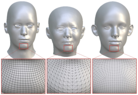
Figure 1.
An example of input model and target models with different topologies and vertices.
After the problem of shape correspondence has been solved, facial blendshapes can be obtained by interpolating and blending available facial models to create new facial shapes. From a shape interpolation point of view, the blend shape methods can be divided into linear and nonlinear interpolation [14]. Among them, linear interpolation [15,16,17] plays a leading role in facial blendshapes. In this paper, we consider linear interpolation-based facial blendshapes.
Since linear interpolation is purely geometric and does not involve any underlying physics of facial deformations, linear interpolation-based facial blendshapes cannot create as realistic facial deformations as physics-based facial blendshapes. The existing physics-based facial blendshapes [18] involve heavy numerical calculations and are not applicable to the situations requiring high performance. PDE-based surfaces have a potential to be developed into an efficient method of physics-based facial blendshapes, which will be investigated in our following work. In addition, linear interpolation-based facial blendshapes interpolate and blend each of the vertices of polygon models, leading to many interpolation and blending operations. This paper will tackle this problem by transforming polygon models into PDE surfaces for interpolating and blending facial models to create facial blendshapes.
2.2. Differential Equation Based Modelling
Differential equation-based modelling can be divided into Ordinary Differential Equation (ODE)-based geometric modelling [19,20] and Partial Differential Equation (PDE)-based geometric modelling [21]. ODE-based modelling is used in C2 continuous surface creation [22] and dynamic skin deformations [23,24]. Since ODE modelling involves one parametric variable, how to manipulate surfaces in two-dimensional regions requires further investigations. PDE-based modelling involves two parametric variables and is more powerful when dealing with more difficult situations.
PDE-based geometric modelling was pioneered by Bloor and Wilson [25] in 1989. Since its advent three decades ago, it has found applications in a lot of surface modelling tasks, including free-form surface generation, n-sided patch modelling, surface blending, and industrial applications, as reviewed by Gonzalez et al. [26]. After that, PDE-based geometric modelling has also been used for facial geometric parameterization [27]. Recently, an optimal NURBS conversion of PDE surface representations was investigated [28].
Compared with the conventional surface modelling methods, the PDE-based methods provide users with a higher level control of the shape of the generated surfaces by using PDE parameters and the boundary conditions instead of many hundreds of control points. Therefore, they can be easily implemented as an easy-to-use interactive modelling user interface. One problem for PDE-based modelling is how to solve partial differential equations. The Fourier series method proposed by Wilson [29] is efficient but applicable to simple surface modelling tasks. For complicated problems, only expensive numerical methods can be used, such as the finite element method, finite difference method, and collocation point method [30].
Although PDE-based modelling has been well investigated, PDE surface-based facial blendshapes have not been addressed. In this paper, we propose a second-order partial differential equation and investigate its Fourier series-based analytical solution. With the obtained analytical solution, we derive the mathematical function of PDE surfaces and use the obtained PDE surface to achieve interpolation-based and blending-based facial blendshapes.
3. Algorithm Overview
As shown in Figure 2, our proposed algorithm consists of three parts. They are PDE surface creation, PDE surface interpolation, and PDE surface blending, which are shown in the top red box, left bottom green box, and right bottom purple box, respectively.
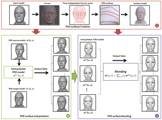
Figure 2.
Algorithm overview.
In the part of PDE surface creation to be investigated in Section 4 below, all the PDE surface patches defining a polygon model are created through the following steps:
(1) A surface patch template is designed to segment a canonical 3D head model into surface patches, each of which is defined by its encircled boundary curves.
(2) When a new head model is input, we match the standard 3D head model with the input model. Accordingly, the template is transferred to the input model to extract the boundary curves. The details of curve extraction are given in Section 4.1.
(3) These extracted boundary curves are described with Fourier series representations of the parametric variable v, as shown by Equations (13) and (14) in Section 4.2.
(4) A second-order partial differential equation subjected to the constraint of the extracted boundary curves is used to create PDE surface patches. The solution of the second-order partial differential equation is a function of parametric variables u and v. Since Fourier series can approximate mathematical functions very well, we propose a generalized Fourier series function involving the parametric variable v and the unknown functions of the parametric variable u as the solution to the second-order partial differential equation. By making the generalized Fourier series function exactly satisfy the second-order partial differential equation, we obtain the unknown functions involved in the generalized Fourier series function. After that, the unknown constants that involved the generalized Fourier series function are determined by making a generalized Fourier series function pass the boundary curves at the starting pose and ending pose.
After all the extracted boundary curves have been used to create PDE surface patches, the original polygon model is changed into PDE surface patches defined as an analytical mathematical expression, i.e., Equation (19).
In the part of PDE surface interpolation to be examined in Section 5, one source model and one target model are interpolated to create intermediate shapes. We first use and to indicate the source model and the target model, respectively. Then, a linear interpolation is used to interpolate and , where and are given in Equations (20) and (21), respectively. The interpolation operation generates a new mathematical function of the interpolated PDE surface patches, which is given in Equation (25). The new mathematical function is used to create many intermediate shapes between the source facial model and the target facial model. Each of the created intermediate shapes is called an interpolated PDE model.
In the part of PDE surface blending to be discussed in Section 6, a blending operation is used to obtain a blend shape . If one source model and target models are to be blended together, PDE surface interpolation is first used to obtain interpolated PDE models by interpolating one source model and a target model . Then, the interpolated PDE models are blended together through Equation (27) to obtain a blend shape whose analytical mathematical expression is given in Equation (29) with its coefficients determined by Equation (28) as weighted combinations of the coefficients in . The obtained blend shape is used to create facial blendshapes and facial animation from the source model and target models . By changing the weights in Equation (27) to generate different combinations, different facial models are created with Equation (29).
4. Curve Extraction and PDE Surfaces
4.1. Extracting Correspondent Curves from 3D Models
In order to create blendshapes between source and target models with different topologies and vertices, first we establish the corresponding relationship between them by extracting correspondent curves. The most common method is to use some horizontal planes to cut the 3D face models and use the intersection curves as the corresponding curves of the source and target models. However, this can lead to problems of inaccuracy because human faces are different, and it is difficult to accurately determine the corresponding positions of the horizontal planes. Therefore, we design a face fragmentation template to fit each of the face models and extract the curves by choosing the points of the models nearest to the wireframe.
As shown in Figure 3, 68 facial landmark points shown in (a) and facial muscles shown in (b) are taken as references. According to the setting in Figure 3, we design a canonical 3D face curve template.
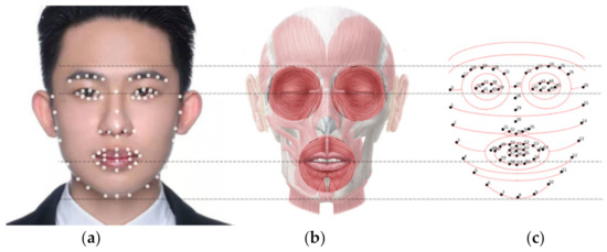
Figure 3.
The curves designed to divide a canonical 3D face model into patches, (a) face photo with 68 landmark points, (b) anatomical diagram of facial muscles, (c) a concept sketch of face curves designed using landmark points and the anatomical diagram as references.
Figure 4 shows one design of facial correspondent curves. The top row of Figure 4 shows the extracted curves from the curve template, and the bottom row shows the positions of the extracted curves on the facial models. The shape of the eye patches is based on the structure of the orbicularis oculi muscle and the shape of the mouth patch is based on orbicularis oris muscle. Similarly, the ear and nostril structures also use vertical oval ripples to fit the face model. Then, the head is divided into sections by two adjacent curves.
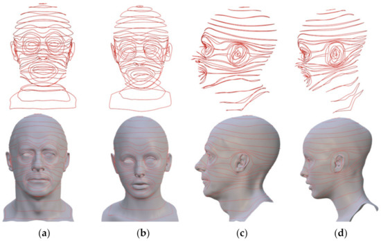
Figure 4.
Front and side view of the design of the curves dividing a canonical 3D face model into patches, (a,c) are a source male face model, (b,d) are a target female face model.
Next, the extracted curves from a source model and a target model are represented with time-independent Fourier series expressions. After that, each of the time-independent Fourier series expressions is introduced into the solution to a selected vector-valued second-order partial differential equation to create curves-defined PDE surfaces, which are used to rebuild the 3D models. By doing so, we convert the correspondence between vertices of polygon models into the correspondence between the extracted curves. The extracted curves are represented with Fourier series in the form of Equation (13) to benefit the following interpolation and blending operations.
4.2. Generating Curve-Defined and Fourier Series-Represented PDE Surfaces
As shown in Figure 5, the extracted curves are discrete points. For the purpose of avoiding the correspondence problem between the curve points of two or more curves, the curves are represented with time-dependent Fourier series according to whether the curves to be represented are closed. With the Fourier series representations, the correspondence between the curve points becomes the correspondence between the same values of the parametric variable in the Fourier series representations.
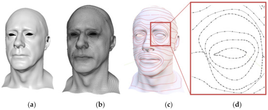
Figure 5.
Extracting correspondent curves from 3D models. (a) Male model (mesh), (b) male model (with wireframe), (c) face model (with extracted curves), (d) local view of the extracted curves in the left eye area.
The following second-order partial differential equation (PDE) is used to define each surface between two adjacent curves.
where is a vector-valued function, which has three components , , and . Since Fourier series can be used to approximate an arbitrary function, we take the solution of PDE (1) to be the following Fourier series representation of the parametric variable whose coefficients are unknown functions of the parametric variable .
where , , and have vector-valued unknown functions. Each of them has three components, for example, , , and .
Substituting Equation (2) into Equation (1), we obtain
From Equation (3), we obtain
where and are two unknown vector-valued constants.
From Equation (4), we obtain
Letting
and substituting Equation (8) into (7), we get
If , we let and obtain . Substituting back to Equation (8), the following equation is obtained
where and are unknown vector-valued constants.
If , If we let , we have . Substituting it into Equation (8), the following equation is obtained
From Equation (5), we get
Similarly, the following equation is obtained for .
where and are unknown vector-valued constants, and the following equation is reached for .
For , Equations (6), (7), and (9) are combined together to give
For , putting Equations (6), (7), and (10) together gives
The boundary curves of a PDE surface are two adjacent extracted curves and , which are defined with the following Fourier series.
where and
- are two vector-valued functions,
- ,
- ,
- ,
- ,
- , and
- are vector-valued unknown constants.
Here, we take Equation (12) to demonstrate how to determine the unknown coefficients from the above two boundary curves. The unknown constraints and in Equation (12) can be determined from the following boundary conditions.
Substituting Equation (12) into the above equations, we obtain
From the above two equations, we have
Solving the above equations, we obtain
Substituting Equation (18) into Equation (12), the PDE surface defined by the boundary curves and is:
The same method can be used to derive the PDE surface for λ/β > 0.
According to the above equation, the extracted curves can be represented by time-independent Fourier series expressions, and the PDE surface patches can be defined by the curves. In other words, the source and target models now have the same Fourier series representation. Then, without changing the topological structure of the model, the non-vertex semantic correspondence between models is now transformed into the correspondence between the corresponding 3D PDE surfaces. Subsequently, the models are ready for generating intermediate blend shapes, as demonstrated in the next section.
5. Facial Blendshapes by Interpolating PDE Surfaces of One Source and One Target Model
With the obtained mathematical representation (19) of PDE surfaces, we can develop a new PDE surface interpolation method to obtain facial blendshapes between one source model and one target model. In what follows, we investigate this approach.
We use w0 (u, v) to indicate one PDE surface patch on one source facial model and w1 (u, v) to indicate the corresponding PDE surface patch on one target facial model. From Equation (19), w0 (u, v) has the form of
and
New facial models can be created by interpolating the PDE surface patches and for all the PDE surface patches on the source and target facial models. There are various interpolation methods, including geometric and physics-based interpolation methods. PDE surfaces provide a good representation for physics-based interpolation. Physics-based interpolation using PDE surfaces will be investigated in our subsequent work. This paper mainly focuses on geometric interpolation. Geometric interpolation can be divided into linear and nonlinear interpolation. Between them, linear interpolation is more popular. Here, we use linear interpolation to derive the mathematical expression of PDE surface interpolation.
We use to indicate a new PDE surface, which is obtained by linearly interpolating the source PDE surface patch and the target surface patch . The linear interpolation can be formulated as
From , , we obtain . From , , we obtain . Considering , we obtain . Substituting the obtained and into Equation (22), we obtain
Substituting Equations (20) and (21) into the above equation and introducing the following notations
Equation (23) becomes
Setting t in Equation (25) to different values in the range , new PDE surfaces are created. Figure 6 shows such an example. In the figure, (d) and (a) depict a source PDE surface patch and its boundary curves, and (e) and (c) show a target PDE surface and its boundary curves. Using Equation (25) and setting t to 0.5, we obtain the blended PDE surface patch shown in Figure 6b.
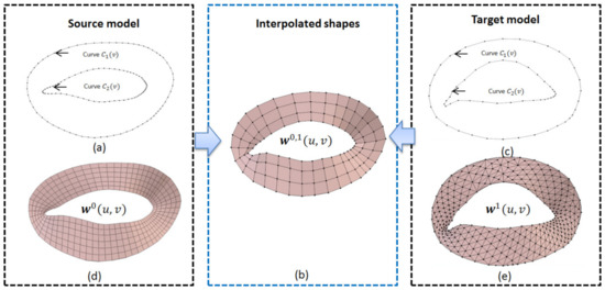
Figure 6.
New created PDE surface patch depicted in (b), which was obtained by using Equation (25) to interpolate the source PDE surface patch in (d) and the target PDE surface patch in (e), where (a) shows the boundary curves of the source PDE surface patch in (d), and (c) depicts the boundary curves of the target PDE surface patch in (e).
If a source facial model consists of PDE surface patches ) and the corresponding PDE surface patches on the target facial model is ) (i = 1,2,3,,, we can obtain new PDE surface patches from Equation (25). All these new PDE surface patches are automatically connected together, and no manual operations are required to stitch them.
Since two adjacent PDE surface patches ) and ) on the source facial model share one common boundary curve, i.e., )=) and two adjacent PDE surface patches ) and ) on the target facial model share another common boundary curve, i.e., )=), after using Equation (25) to do the linear interpolation, the two adjacent PDE surface patches and on interpolated facial models also share a common boundary curve, as explained below.
On the common boundary, we have and . Since )=) and )=), we have . Therefore, the two adjacent PDE surface patches and share a common boundary curve. That is to say, the new created facial models keep positional continuity between two adjacent facial models obtained from Equation (25).
Figure 7 gives four examples of using Equation (25) to created new facial models from one source facial model and one target facial model, which have different numbers of vertices. In the figure, the left column shows four source facial models and the right column depicts four target facial models. Setting in Equation (25) to different values in the region , we create many new facial models. In the figure, the four middle facial models are the new created facial models at t = 0.2, 0.4, 0.6, and 0.8.
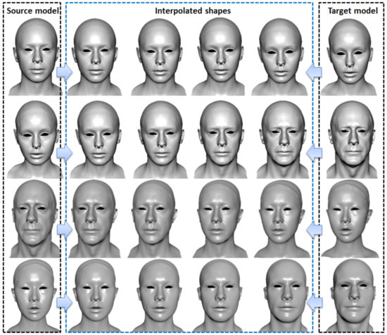
Figure 7.
Facial models created by using Equation (25) to interpolate source facial models and target facial models, where the left column shows four source facial models, the right column depicts four target facial models, and the four middle facial models on each of the four rows are new created facial models by setting t = 0.2, 0.4, 0.6, and 0.8 in Equation (25).
From Figure 7, we can see that as increases from to , the source facial models shown in the left column gradually change their shapes and finally become the target facial models shown in the right column. It demonstrates the correctness of Equation (25).
Unlike traditional linear interpolation of polygon models, which interpolates each of many vertices of a source facial model and a target facial model, the proposed method only interpolates the coefficients of Equation (25) for a few PDE surface patches of a source and a target facial model.
6. Facial Blendshapes by Blending PDE Surfaces of One Source and Many Target Facial Models
In comparison with facial blendshapes by interpolating one source facial model and one target facial model, facial blendshapes by blending one source facial model and more than one target facial models can create much more new facial models. Such a method of facial blendshapes is widely applied in creating detailed facial animation. In this section, we investigate this method.
If one source facial model and target facial models are to be blended together, for one PDE surface patch on the source facial model and the corresponding PDE surface patch on the target facial model, we can obtain from Equation (25), which interpolates PDE surface patches on the source facial model and the corresponding PDE surface patches on the target facial model. After this treatment, blending the source facial model and target facial models is transformed into blending .
For the polygon representation of facial models, the existing method of facial blendshapes directly blends the vertices of these models together. If one of the source facial models and the target facial models have vertices and each vertex has three components , , and , we put the components , , and for all vertices into a column vector . The blend shape is expressed as [1]
where is called a weight satisfying and , and indicates the source model.
Unlike the above method, which blends many vertices of polygon facial models, the method to be proposed below only blends the analytical mathematical expressions of the PDE surface patches, which represent the same facial models as the polygon facial models. The fundamental equation is similar to Equation (26), i.e.,
Substituting Equation (25) into the above equation and letting
we obtain
Using the above Equation (29), we can create many new facial models from one source facial model and many target facial models. Figure 8 gives an example. In the figure, one source facial model and three target facial models are shown in the left box and the right box shows the created new model.
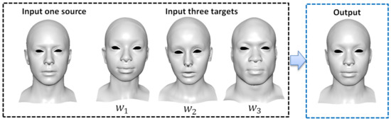
Figure 8.
Facial blendshapes by using Equation (29) to blend PDE surface patches on one source facial model and three target facial models with , , , and .
Figure 8 indicates that with the combination of the weights , , and , a blendshape can be correctly created by using Equation (29) to blend the source facial model and three target facial models together. It demonstrates the correctness of the proposed blending operation, i.e., Equation (29).
As shown in Table 1, interpolating the first (source) facial model and the second (target) facial model from the left in Figure 8 involves interpolating 31,331 vertices. In contrast, interpolating their corresponding PDE surfaces inly involves 6534 coefficients of Equation (25). It indicates that the total number of interpolation operations for polygon models are about five times of the total number of the interpolation operations for the corresponding PDE surfaces.

Table 1.
Comparison of design variables between polygon models and their PDE surface representations.
Table 1 above gives a comparison of the design variables of polygon models and the corresponding PDE surfaces. The design variables are the vertices for polygon models and the coefficients involved in Equation (25) for the corresponding PDE surfaces. In the table, the second column indicates the source facial model, which is the first model from the left of Figure 8, the third, fourth, and fifth columns denote the first, second, and third target facial models, which are the second, third, and fourth models from the left of Figure 8, the second and third rows give the total vertex number and total face number for each of the polygon models shown in Figure 8, and the fourth row gives the total coefficient number of PDE surfaces representing the corresponding polygon models.
Similar to the comparison between the traditional linear interpolation of polygon models and linear interpolation of PDE surfaces, Table 1 indicates that the total number of the blending operations for polygon models, which blend the vertices of polygon models, are about five times the total number of the blending operations for PDE surfaces, which use Equation (28) to blend the coefficients in Equation (25).
Using different combinations of , , and will lead to different facial models to be created. Here, we use three different combinations to demonstrate this. These three combinations are (1) , , and ; (2) , , and ; and (3) , , and . The new created facial models at , , , , and are shown in Figure 9 for the first combination, Figure 10 for the second combination, and Figure 11 for the third combination.
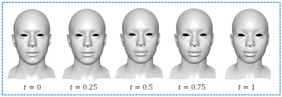
Figure 9.
Facial blendshapes created by using Equation (29) with , , and .
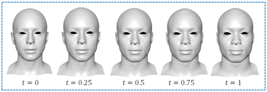
Figure 10.
Facial blendshapes created by using Equation (29) with , , and .
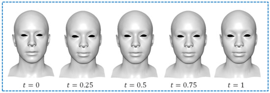
Figure 11.
Facial blendshapes created by using Equation (29) with , , and .
Figure 9, Figure 10 and Figure 11 indicate that the proposed approach successfully blends one source facial model with the 31,331 vertices and three target facial models with 31,331, 38,802, and 34,068 vertices to create new blendshapes. It demonstrates the benefit of the proposed approach in blending facial models with different vertices.
In order to quantify the quality of the reconstructed PDE surfaces, we calculate the maximum errors (ErM) and average errors (ErA) between the reconstructed PDE surfaces and the original polygon model with the following error metrics
In the above equation, is the total number of the vertices in the area of a polygon model corresponding to a PDE surface patch, is the distance between the two most distant points on the model, and is determined by
where , , and are the , , and coordinate values of the vertex on the polygon model, and , and are the , , and coordinate values of the points on the PDE surface patch corresponding to the vertex on the polygon model.
The errors between the reconstructed PDE surfaces and the original polygon model obtained with Equation (30) are given in Table 2. In the table, is defined in Equation (2).
Table 2.
Errors between the reconstructed PDE surfaces and the original polygon model.
Table 2 indicates how the maximum and average errors reduce with the increase in the Fourier series terms . Even when few terms of the Fourier series are used, i.e., , the maximum and average errors are 0.06681861 and 0.02264859 only, which are small. When is increased from to , both the maximum and average errors are greatly reduced. As the terms of the Fourier series continue to increase, the maximum and average errors are further reduced.
Facial animation can be created by animating the created facial blendshapes. Using Equation (29) to calculate new blendshapes from more combinations, we obtain more facial shapes and use them to create facial animation, as shown in the accompanied video.
7. Conclusions
In this paper, we have developed a new method of facial blendshapes for creating new facial blendshapes and generating face animation. We have proposed a curve template to extract curves from polygon facial models, used extracted curves to define the boundaries of PDE surface patches, and solved a second-order partial differential equation subjected to the constraints of the extracted boundary curves represented with Fourier series to obtain the mathematical expression of curve-defined and Fourier series-represented PDE surfaces. Using the obtained PDE surfaces, we have developed the analytical mathematical expression of PDE surface interpolation, which interpolates one source facial model and one target facial model to create new facial shapes. We have also used the obtained analytical mathematical expression of PDE surface interpolation to achieve the analytical mathematical expression of PDE surface-based facial blendshapes, which blends one source facial model and many target facial models to create new facial blendshapes and generate facial animation. Some examples have been presented to demonstrate the correctness of the obtained mathematical expressions and the applications in facial blendshapes and facial animation.
In this paper, we only investigate PDE surface-based facial blendshapes. Actually, the obtained mathematical expressions of curve-defined and Fourier series-represented PDE surfaces, PDE surface interpolation, and PDE surface blending are also applicable to any other models with different topologies and/or different vertices once the correct correspondence between PDE surface patches is obtained. We will extend the work given in this paper to blendshapes of other models and different types of models.
Linear interpolation was used in this paper to create new facial models and facial animation from one source facial model and one target facial model. Physics-based interpolation can create more realistic appearances and PDE surfaces are especially applicable to the development of physics-based interpolation. Thus, in our following work, we will introduce physics-based interpolation into PDE surfaces to replace linear interpolation.
Polygon models are represented by many discrete vertices, which are not applicable to some applications’ level of detail (LOD) due to their fixed resolutions and machine learning-related situations due to too many vertices. PDE surfaces are represented with an analytical mathematical expression and can easily achieve many different levels of detail for applications in the situations requiring a level of detail. In addition, the coefficients involved in the analytical mathematical expression of the PDE surfaces used to represent a polygon model are far fewer than the vertices of the polygon model, which makes the analytical mathematical expression of PDE surfaces applicable to machine learning-related situations. We will also investigate these problems in our following work.
The limitation of this approach is the reconstructed PDE models have some small errors compared with the original models. However, this could be minimized by increasing until the errors could be negligible. This method works well on complicated head models. However, it is not suitable for some models with no volume or thickness such as four-sided patches. We will extend the approach proposed in this paper to tackle these models and make PDE surface-based facial blendshapes able to deal with all the models, which can be dealt with by interpolation-based facial blendshapes of polygon models reviewed in [1].
In the future, we will also examine how to optimize the patch design and apply the obtained curve-defined and Fourier series-represented PDE surfaces to tackle more problems such as rigid and non-ridged registration, deformation transfer, self-similarity detection, and time-dependent surface reconstruction.
Author Contributions
Conceptualization, L.Y. and H.F.; validation, S.B., E.C. and S.W.; writing—original draft preparation, H.F.; writing—review and editing, H.F., S.B. and L.Y.; visualization, H.F.; supervision, L.Y. and J.J.Z.; funding acquisition, L.Y. and J.J.Z. All authors have read and agreed to the published version of the manuscript.
Funding
This research is supported by the PDE-GIR project, which has received funding from the European Union Horizon 2020 Research and Innovation Programme under the Marie Skodowska-Curie grant agreement No 778035. And Haibin Fu is grateful for a scholarship from the Rabin Ezra Scholarship Trust.
Institutional Review Board Statement
Not applicable.
Informed Consent Statement
Not applicable.
Data Availability Statement
Not applicable.
Conflicts of Interest
The authors declare no conflict of interest.
References
- Lewis, J.; Anjyo, K.; Rhee, T.; Zhang, M.; Pighin, F.; Deng, Z. Practice and theory of blendshape facial models. Eurograph. Assoc. 2014, 8, 2. [Google Scholar]
- Alexa, M. Recent advances in mesh morphing. Comput. Graph. Forum 2002, 21, 173–198. [Google Scholar] [CrossRef]
- Seo, J.; Irving, G.; Lewis, J.P.; Noh, J. Compression and direct manipulation of complex blendshape models. ACM Trans. Graph. 2011, 30, 1–10. [Google Scholar] [CrossRef] [Green Version]
- Flueckiger, B. Computer-Generated Characters in Avatar and Benjamin Button; Letzler, B., Ed.; Digitalitat und Kino: Munich, Germany, 2011. [Google Scholar]
- You, X.; Tian, F.; Tang, W. Highly efficient facial blendshape animation with analytical dynamic deformations. Multimed. Tools Appl. 2019, 78, 25569–25590. [Google Scholar] [CrossRef]
- Van Kaick, O.; Zhang, H.; Hamarneh, G.; Cohen-Or, D. A Survey on Shape Correspondence. Comput. Graph. Forum 2011, 30, 1681–1707. [Google Scholar] [CrossRef] [Green Version]
- Rusinkiewicz, S.; Marc, L. Efficient variants of the ICP algorithm. In Proceedings of the Third International Conference on 3-D Digital Imaging and Modeling, Quebec City, QC, Canada, 28 May–1 June 2001; pp. 145–152. [Google Scholar]
- Xu, K.; Zhang, H.; Tagliasacchi, A.; Liu, L.; Li, G.; Meng, M.; Xiong, Y. Partial intrinsic reflectional symmetry of 3D shapes. ACM Trans. Graph. 2009, 28, 1–10. [Google Scholar] [CrossRef] [Green Version]
- Seibold, C.; Samek, W.; Hilsmann, A.; Eisert, P. Accurate and robust neural networks for face morphing attack detection. J. Inf. Secur. Appl. 2020, 53, 102526. [Google Scholar] [CrossRef]
- Liu, M.; Sheng, L.; Yang, S.; Shao, J.; Hu, S.-M. Morphing and Sampling Network for Dense Point Cloud Completion. Proc. AAAI Conf. Artif. Intell. 2020, 34, 11596–11603. [Google Scholar] [CrossRef]
- Ma, W.-C.; Ma, C.; Lamarre, M.; Danvoye, E.; Ko, M.; Von Der Pahlen, J.; Wilson, C. Semantically-aware blendshape rigs from facial performance measurements. Siggraph Asia Tech. Briefs 2016, 3, 1–4. [Google Scholar] [CrossRef]
- Chen, K.; Zheng, J.; Cai, J.; Zhang, J. Modeling Caricature Expressions by 3D Blendshape and Dynamic Texture. In Proceedings of the 28th ACM International Conference on Multimedia, Seattle, WA, USA, 12–16 October 2020. [Google Scholar] [CrossRef]
- Van Kaick, O.; Tagliasacchi, A.; Sidi, O.; Zhang, H.; Cohen-Or, D.; Wolf, L.; Hamarneh, G. Prior Knowledge for Part Correspondence. Comput. Graph. Forum 2011, 30, 553–562. [Google Scholar] [CrossRef] [Green Version]
- Liu, X.; Xia, S.; Fan, Y.; Wang, Z. Exploring Non-Linear Relationship of Blendshape Facial Animation. Comput. Graph. Forum 2011, 30, 1655–1666. [Google Scholar] [CrossRef]
- Sifakis, E.; Neverov, I.; Fedkiw, R. Automatic determination of facial muscle activations from sparse motion capture marker data. ACM Trans. Graph. 2005, 24, 417–425. [Google Scholar] [CrossRef]
- Tena, J.R.; De la Torre, F.; Matthews, I. Interactive region-based linear 3D face models. ACM Trans. Graph. 2011, 76, 1–10. [Google Scholar] [CrossRef]
- Vlasic, D.; Brand, M.; Pfister, H.; Popović, J. Face transfer with multilinear models. ACM Trans. Graph. 2005, 24, 426. [Google Scholar] [CrossRef]
- Barrielle, V.; Stoiber, N.; Cagniart, C. Blendforces: A dynamic framework for facial animation. Comput. Graph. Forum 2016, 35, 341–352. [Google Scholar] [CrossRef]
- Liang, H.; Chang, J.; Yang, X.; You, L.; Bian, S.; Zhang, J.J. Advanced ordinary differential equation based head modelling for Chinese marionette art preservation. Comput. Animat. Virtual Worlds 2015, 26, 207–216. [Google Scholar] [CrossRef]
- Bian, S.; Deng, Z.; Chaudhry, E.; You, L.; Yang, X.; Guo, L.; Ugail, H.; Jin, X.; Xiao, Z.; Zhang, J.J. Efficient and realistic character animation through analytical physics-based skin deformation. Graph. Models 2019, 104, 101035. [Google Scholar] [CrossRef]
- You, L.; Yang, X.; Pan, J.; Lee, T.-Y.; Bian, S.; Qian, K.; Habib, Z.; Sargano, A.B.; Kazmi, I.; Zhang, J.J. Fast character modeling with sketch-based PDE surfaces. Multimed. Tools Appl. 2020, 79, 23161–23187. [Google Scholar] [CrossRef]
- Bian, S.; Maguire, G.; Kokke, W.; You, L.; Zhang, J.J. Efficient C2 Continuous Surface Creation Technique Based on Ordinary Differential Equation. Symmetry 2019, 12, 38. [Google Scholar] [CrossRef] [Green Version]
- Bian, S.; Zheng, A.; Chaudhry, E.; You, L.; Zhang, J. Automatic Generation of Dynamic Skin Deformation for Animated Characters. Symmetry 2018, 10, 89. [Google Scholar] [CrossRef] [Green Version]
- Chaudhry, E.; Bian, S.J.; Ugail, H.; Jin, X.; You, L.H.; Zhang, J.J. Dynamic skin deformation using finite difference solutions for character animation. Comput. Graph. 2015, 46, 294–305. [Google Scholar] [CrossRef] [Green Version]
- Bloor, M.; Michael, W. Using partial differential equations to generate free-form surfaces. Comput.-Aided Des. 1990, 22, 202–212. [Google Scholar] [CrossRef]
- Castro, G.G.; Athanasopoulos, M.; Ugail, H. Cyclic animation using Partial differential Equations. Vis. Comput. 2010, 26, 325–338. [Google Scholar] [CrossRef] [Green Version]
- Sheng, Y.; Willis, P.; Castro, G.G.; Ugail, H. Facial geometry parameterisation based on Partial Differential Equations. Math. Comput. Model. 2011, 54, 1536–1548. [Google Scholar] [CrossRef] [Green Version]
- Wang, S.; Xia, Y.; Wang, R.; You, L.; Zhang, J. Optimal NURBS conversion of PDE surface-represented high-speed train heads. Optim. Eng. 2019, 20, 907–928. [Google Scholar] [CrossRef] [Green Version]
- Ugail, H.; Bloor, M.I.G.; Wilson, M.J. Techniques for interactive design using the PDE method. ACM Trans. Graph. 1999, 18, 195–212. [Google Scholar] [CrossRef]
- Babuška, I.; Nobile, F.; Tempone, R. A Stochastic Collocation Method for Elliptic Partial Differential Equations with Random Input Data. SIAM J. Numer. Anal. 2007, 45, 1005–1034. [Google Scholar] [CrossRef]
Publisher’s Note: MDPI stays neutral with regard to jurisdictional claims in published maps and institutional affiliations. |
© 2021 by the authors. Licensee MDPI, Basel, Switzerland. This article is an open access article distributed under the terms and conditions of the Creative Commons Attribution (CC BY) license (https://creativecommons.org/licenses/by/4.0/).