Article

On Some Features of the Numerical Solving of Coefficient Inverse Problems for an Equation of the Reaction-Diffusion-Advection-Type with Data on the Position of a Reaction Front

1
Department of Mathematics, Faculty of Physics, Lomonosov Moscow State University, 119991 Moscow, Russia
2
Moscow Center for Fundamental and Applied Mathematics, 119234 Moscow, Russia
3
Institute of Computational Mathematics and Mathematical Geophysics of SB RAS, 630090 Novosibirsk, Russia
4
Department of Mathematics and Mechanics, Novosibirsk State University, 630090 Novosibirsk, Russia
*
Author to whom correspondence should be addressed.
Mathematics 2021, 9(22), 2894; https://doi.org/10.3390/math9222894
Submission received: 13 October 2021 / Revised: 8 November 2021 / Accepted: 12 November 2021 / Published: 13 November 2021
(This article belongs to the Section Computational and Applied Mathematics)

Abstract

:
The work continues a series of articles devoted to the peculiarities of solving coefficient inverse problems for nonlinear singularly perturbed equations of the reaction-diffusion-advection-type with data on the position of the reaction front. In this paper, we place the emphasis on some problems of the numerical solving process. One of the approaches to solving inverse problems of the class under consideration is the use of methods of asymptotic analysis. These methods, under certain conditions, make it possible to construct the so-called reduced formulation of the inverse problem. Usually, a differential equation in this formulation has a lower dimension/order with respect to the differential equation, which is included in the full statement of the inverse problem. In this paper, we consider an example that leads to a reduced formulation of the problem, the solving of which is no less a time-consuming procedure in comparison with the numerical solving of the problem in the full statement. In particular, to obtain an approximate numerical solution, one has to use the methods of the numerical diagnostics of the solution’s blow-up. Thus, it is demonstrated that the possibility of constructing a reduced formulation of the inverse problem does not guarantee its more efficient solving. Moreover, the possibility of constructing a reduced formulation of the problem does not guarantee the existence of an approximate solution that is qualitatively comparable to the true one. In previous works of the authors, it was shown that an acceptable approximate solution can be obtained only for sufficiently small values of the singular parameter included in the full statement of the problem. However, the question of how to proceed if the singular parameter is not small enough remains open. The work also gives an answer to this question.

1. Introduction

Nonlinear singularly perturbed reaction–diffusion–advection equations arise when solving the problems in gas dynamics [1], combustion theory [2], chemical kinetics [3,4,5,6,7,8,9], nonlinear wave theory [10], biophysics [11,12,13,14,15], medicine [16,17,18,19], ecology [20,21,22], finance [23], and other areas of science [24]. Inverse problems for the equation of this type often arise when solving various applied problems and consist of recovering some coefficient in the equation. To solve inverse problems, it is necessary to have additional information about the solution of the equation. Most often, such additional information is information about the solution on a part of the boundary of the domain on which the equation is considered (see, for example, [25,26,27,28,29,30,31,32,33,34,35]). However, recently, the formulation of inverse problems for the equation of this type with additional information on the dynamics of the reaction front has become relevant because the reaction front is an experimentally easily distinguishable contrast structure (see, for example, [36,37]).
This work is a continuation of [36,38,39,40,41]. In these works, questions were considered about the possibility of applying the methods of asymptotic analysis [3,42,43,44] to recover some coefficients in inverse problems for nonlinear singularly perturbed reaction–diffusion–advection equations with data on the position of a reaction front. The authors demonstrated approaches on how to reduce the original formulation (full statement) of the inverse problem for a nonlinear singularly perturbed partial differential equation to a much simpler problem with respect to the reconstructed function (coefficient). The problem obtained using the methods of asymptotic analysis is called the reduced formulation of the inverse problem. The authors already showed that the reduced formulations can contain (1) algebraic equations for an unknown coefficient (see, for example, [38,39]), (2) differential equations for an unknown coefficient (see, for example, [40]), and (3) integral equations for an unknown coefficient (see, for example, [41]). It was shown that in the case of sufficiently small values of the singular parameter included in the original partial differential equation, the reduced formulation provides an opportunity to obtain an approximate solution close to the solution of the inverse problem in the full statement. In this case, all the reduced formulations obtained in the indicated works allowed the use of fairly simple algorithms for the numerical solving of the considered problems. In this paper, we want to consider an example that leads to a reduced formulation of the inverse problem, the solution of which is no less a time-consuming procedure compared to the numerical solution of the problem in the full formulation. This is due to the fact that the reduced formulation is reduced to the need to solve a nonlinear boundary value problem for the eigenvalues. Moreover, according to the results of [39,40,41], the question of what to do in the case when the value of the singular parameter is not small enough remained open. When solving real applied problems, it is often not known in advance whether the singular parameter contained in the problem statement can be considered small enough to apply the approaches from [36,39,40,41]. Can the solution obtained by the methods from [36,39,40,41] be defined more precisely? We give an answer to this question as well.
The already mentioned feature of the reduced formulation of the inverse problem is the need to solve nonlinear boundary value problems for the eigenvalues. These eigenvalues will determine the unknown coefficient pointwise. Classical approaches to solving the obtained problem, for example, the shooting method, are inapplicable. This is due to the fact that the Cauchy problem arising in the implementation of the shooting method may not have a solution for some numerical approximations of the desired coefficient. The question arises: Is it possible to diagnose the absence of a solution to such an auxiliary problem and use this information to construct an effective numerical algorithm in order to find the solution? The absence of a solution to the Cauchy problem arising in the shooting method is due to the fact that the norm of the derivative of the solution tends to infinity on a finite set. Therefore, this problem belongs to the “blow-up” problems’ class. To date, there are three main groups of methods for the analytical study of the phenomena of the solution’s blow-up. These are the method of nonlinear capacity (trial functions) [45] in various versions, the energy method and its modifications [46,47,48], and the method of self-similar modes, based on various comparison criteria, developed in [49,50]. All these methods can only give a rough estimate for the desired parameter of the blow-up. Therefore, numerical diagnostics of the existence of a solution to the corresponding Cauchy problem becomes relevant. Problems of this type are complex, and there is an extensive literature devoted to them. Thus, adaptive approaches are often used, associated with a decrease in the grid step (in time and, possibly, in space) [51,52] and with a posteriori estimates [52]. These include methods based on the transition from a temporary variable to an expanded variable [53], for example, to the length of the graph arc. In some cases, the solution is scaled as it grows [54]. The method for diagnosing the existence of a solution used in this work is based on the idea of the a posteriori accuracy estimate. Its main ideas were outlined in [55,56]. In short, on a smooth solution, the effective order of accuracy tends to be the theoretical one for the given scheme; hence, a sharp change in the effective order of accuracy indicates the solution’s blow-up. Conceptually, the method of [57] is close to it, which diagnoses the blow-up by the growth of the residual of a numerical solution when the grid parameter tends to zero (for a smooth solution, the residual must decrease). The application of these approaches makes it possible to construct a numerical algorithm for solving the inverse problem in a reduced formulation.
The structure of this paper is as follows. Section 2 contains a full statement of the inverse problem under consideration. Section 2.2 contains a reduced formulation of the inverse problem resulting from the application of asymptotic analysis methods. In Section 2.3, a numerical algorithm for solving the reduced problem, based on the method of numerical diagnostics of the solution’s blow-up, is discussed in detail. Section 2.4 contains numerical experiments demonstrating the applicability of the proposed approach to solving the inverse problem considered in this work. At the same time, an example is also demonstrated for the case of an insufficiently small value of the singular parameter, for which the approach based on the use of methods of asymptotic analysis does not give a satisfactory result. Section 3.1 contains a modified formulation of the inverse problem, which allows applying a solution method based on minimizing the target functional. Section 3.2 contains the formulas for the gradient minimization method. As an initial approximation in the gradient method, the information about the solution obtained by the methods of asymptotic analysis is used. Section 3.3 demonstrates numerical results that support the effectiveness of the proposed approach. In the Conclusion, the features and limitations of the proposed solution method are discussed.

2. Statement of the Inverse Problem and a Method for Its Solution Based on the Results of Applying the Methods of Asymptotic Analysis

2.1. Full Statement of the Inverse Problem

Consider the problem for a nonlinear singularly perturbed reaction–diffusion equation:
ε 2 2 u x 2 ε u t = B u , x , t , q ( t ) , x ( 0 , 1 ) , t ( 0 , T ] , u x ( 0 , t ) = 0 , u x ( 1 , t ) = 0 , t ( 0 , T ] , u ( x , 0 ) = u i n i t ( x ) , x [ 0 , 1 ] .
Here, ε is a small singular parameter and B u , x , t , q ( t ) and u i n i t ( x ) are sufficiently smooth functions. Moreover, the function B u , x , t , q ( t ) for all t [ 0 , T ] has three such simple isolated real roots φ ( ) ( x , t ) , φ ( + ) ( x , t ) , and q ( t ) that φ ( ) ( x , t ) < q ( t ) < φ ( + ) ( x , t ) for all x [ 0 , 1 ] , t [ 0 , T ] .
Under certain conditions (see [58]), the problem (1) can have a solution of a moving-front-type (see Figure 1). A solution of this type is a function that has a narrow inner transition layer in a small (of the order of ε | ln ε | ) neighborhood of some point moving according to the law x = x t . p . ( t ) . We call the point x t . p . ( t ) the “transition point” (“t.p”). Outside this neighborhood, the solution is close to one of two functions, φ ( ) ( x , t ) or φ ( + ) ( x , t ) (see Figure 1a).
The inverse problem is to determine the coefficient q ( t ) , t [ 0 , T ] , in (1) from the known additional information about the position of the reaction front:
x t . p . ( t ) = f 1 ( t ) , t [ 0 , T ] .
Remark 1.
When solving this inverse problem, we use the function of one variable f 1 ( t ) as additional information. Therefore, we can restore only the function of one variable—in our case, the function q ( t ) . If it is necessary to restore the function of two variables q ( x , t ) when setting the corresponding inverse problem, we would need additional information in the form of some function depending on the argument x.
In practice, instead of exact data f 1 ( t ) , their approximate values f 1 δ 1 ( t ) are known (see Figure 1a), estimated experimentally, wherein:
f 1 f 1 δ 1 L 2 δ 1 .
To solve the inverse problem, an explicit connection between the sought function q ( t ) and the data of the inverse problem f 1 ( t ) is required. When constructing a reduced formulation of the inverse problem (Section 2.2) and when using the gradient method for minimizing the target functional (Section 3.1), the following formal definition of the function x = x t . p . ( t ) f 1 ( t ) through the parameters of the problem (1) is used. According to [3,58], the function x = x t . p . ( t ) can be found as a solution of a functional equation (see Figure 1b):
u ( x , t ) = q ( t ) , t [ 0 , T ] .
Remark 2.
According to the formal definition of the function f 1 ( t ) (see Figure 1b), one might get the impression that the required function q ( t ) can be defined in the simplest way, namely, as q ( t ) : = u ( f 1 ( t ) , t ) . However, taking into account possible significant errors in the experimental determination of the values of the function u ( x , t ) lying on the reaction front, this method of restoring the function q ( t ) is incorrect.

2.2. Reduced Statement of the Inverse Problem

The methods of asymptotic analysis [3] make it possible to obtain a representation of the function x t . p . ( t ) in the form:
x t . p . ( t ) = x 0 ( t ) + O ( ε ) .
Here, x 0 ( t ) is the zero approximation for the coordinate of the localization point of the reaction front at time t. The methods of asymptotic analysis [58] allow us to write out the following problem for determining the principal term x 0 ( t ) of the asymptotic approximation in terms of the small singular parameter ε of the exact position x t . p . ( t ) :
d v d u ˜ + d x 0 d t ( t ) = B u ˜ , x 0 ( t ) , t , q ( t ) v , u ˜ φ ( ) x 0 ( t ) , t , φ ( + ) x 0 ( t ) , t , v φ ( ) ( x 0 ( t ) , t ) = 0 , v φ ( + ) ( x 0 ( t ) , t ) = 0 .
According to (3), we can replace in (4) the zero-order term x 0 ( t ) by the function f 1 ( t ) , which determines the position of the reaction front. As a result, we obtain the problem:
d v d u ˜ + d f 1 d t ( t ) = B u ˜ , f 1 ( t ) , t , q ( t ) v , u ˜ φ ( ) f 1 ( t ) , t , φ ( + ) f 1 ( t ) , t , v φ ( ) f 1 ( t ) , t = 0 , v φ ( ) f 1 ( t ) , t = 0 .
Remark 3.
Such replacement is justified only for sufficiently small values of the singular parameter ε (from (3), it follows that x t . p . ( t ) x 0 ( t ) = O ( ε ) ).
Thus, we obtained a reduced formulation (5) of the original inverse problems (1) and (2). This statement connects the function q ( t ) , which must be restored when solving the inverse problem, with the data of the inverse problem—the function f 1 ( t ) , which determines the position of the moving reaction front x t . p . ( t ) f 1 ( t ) measured experimentally.
Remark 4.
The problem (5) (1) does not contain a small parameter and (2) is a nonlinear boundary value problem for eigenvalues with respect to the values of the unknown function q ( t ) at each separate fixed time moment t.

2.3. Numerical Algorithm for Solving the Inverse Problem in the Reduced Statement

In Section 2.2, we obtained a reduced formulation of the problem (5), containing known information about the exact position x t . p . ( t ) f 1 ( t ) of the moving front of the reaction (internal layer). Note again that this problem is an eigenvalue problem to determine the value of q ( t ) for each fixed value of the parameter t. For the convenience of the subsequent numerical solving, we reformulated the problem (5) in the following form: for each value of the parameter t, it is necessary to find a value q ˜ such that the function v ( u ˜ ) , which is a solution to the Cauchy problem:
d v d u ˜ + d f 1 d t ( t ) = B ( u ˜ , f 1 ( t ) , t , q ˜ ) v , u ˜ φ ( ) f 1 ( t ) , t , φ ( + ) f ( t ) , t , v φ ( ) f 1 ( t ) , t = 0 ,
satisfies the condition:
v φ ( + ) f 1 ( t ) , t = 0 .
We denote this value of q ˜ as q ( t ) . It is the desired value.
Remark 5.
When solving the problem (6) numerically, the value of the right-hand side B ( u ˜ , f 1 ( t ) , t , q ( t ) ) / v at the starting point u ˜ = φ ( ) f 1 ( t ) , t is needed. At this point, v ( u ˜ ) = 0 , which gives the uncertainty of the expression B u ˜ , f ( t ) , t , q ( t ) / v . However, in the neighborhood of v ( φ ( ) ) = 0 , we can estimate the value of v ( u ˜ ) with the order of the accuracy equal to O ( u ˜ φ ( ) ) p , p { 1 ; 2 ; 3 ; 4 } [58]:
v ( u ˜ ) = i = 1 p 1 K i u ˜ φ ( ) i + O u ˜ φ ( ) p ,
where:
K 1 = 0.5 V + 0.25 V 2 + B u ˜ u ˜ , f 1 ( t ) , t , q ˜ | u ˜ = φ ( ) , K 2 = 0.5 · B u ˜ u ˜ u ˜ , f 1 ( t ) , t , q ˜ · 0.5 V + 0.25 V 2 + B u ˜ u ˜ , f 1 ( t ) , t , q ˜ B u ˜ u ˜ , x , t , q ˜ + 2 · 0.5 V + 0.25 V 2 + B u ˜ u ˜ , f 1 ( t ) , t , q ˜ 2 | u ˜ = φ ( ) , K 3 = 1 6 · B u ˜ u ˜ u ˜ u ˜ , f 1 ( t ) , t , q ˜ 2 K 2 2 · K 1 B u ˜ u ˜ , f 1 ( t ) , t , q ˜ + 3 K 1 2 | u ˜ = φ ( ) .
When solving the Cauchy problem (6) numerically, due to machine round-off errors, it is impossible to achieve exact fulfillment of the condition (7) at any value of q ˜ . One of the following two cases will always be true:
  • The solution to the Cauchy problem (6) exists throughout the entire area:
    U ˜ φ ( ) f 1 ( t ) , t , φ ( + ) f 1 ( t ) , t .
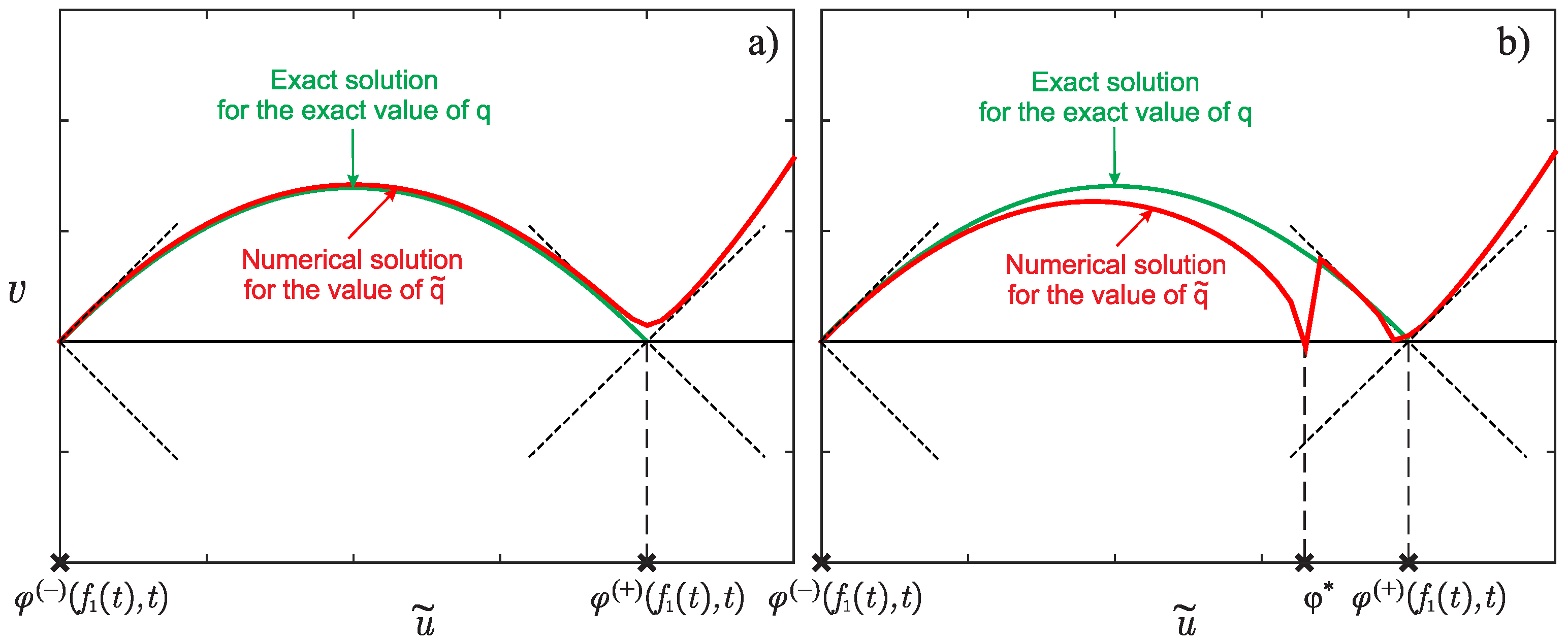
    Moreover, v ( u ˜ ) > 0 for all u ˜ U ˜ , including v φ ( + ) f 1 ( t ) , t > 0 (see Figure 2a);
  • The solution to the Cauchy problem (6) does not exist in the entire domain U ˜ , but only in some subdomain φ ( ) f 1 ( t ) , t , φ * U ˜ , where φ ( ) f 1 ( t ) , t < φ * < φ ( + ) f 1 ( t ) , t , including the values v ( u ˜ ) for u ˜ > φ * , it will not exist (see Figure 2b).
In connection with this feature of the numerical solution of the Cauchy problem (6), we propose the following approach for determining a good approximation for the exact value of q. This approach is a generalization of the dichotomy method. We chose two such values q ( 1 ) and q ( 2 ) where the solution of the Cauchy problem (6) for one of them exists on the whole set U ˜ and for another, where it does not exist on this whole set. Further, by dividing the segment in half, we obtain q ( 3 ) = ( q ( 1 ) + q ( 2 ) ) / 2 and check whether for q ˜ = q ( 3 ) , the solution on the whole set U ˜ exists or not. From two segments q ( 1 ) , q ( 3 ) and q ( 3 ) , q ( 2 ) , choose one for one of the boundary values of which the solution to the Cauchy problem (6) exists on the entire set U ˜ and for another boundary value, which does not exist on this entire set. Continuing the process of dividing the segment in half, we can achieve the convergence of the sequence q ( s ) to the exact value q with a given accuracy.
Thus, it becomes necessary to diagnose the existence of a solution on the entire domain U ˜ . To do this, we used the method of the numerical diagnostics of the existence of a solution based on the method of refining grids [55,56,59,60,61].
The idea of the method is as follows. Let us introduce a basic uniform grid U ˜ N with respect to the variable u ˜ : U ˜ N = { u ˜ n , 0 n N : u ˜ n = φ ( ) f 1 ( t ) , t + h ˜ n , h ˜ = φ ( + ) ( f 1 ( t ) , t ) φ ( ) f 1 ( t ) , t / N } . Suppose that to solve the Cauchy problem (6), we use a scheme with an order of accuracy O ( h ˜ p ) (further, when carrying out numerical experiments, we used a four-stage Runge–Kutta scheme, ERK4, with p = 4 ). First, we performed calculations on the base grid U ˜ N . Then, we refined this grid by an integer number of r and performed calculations on the refined grid U ˜ r N . Continuing the process of refining the grids S 1 times, as a result, we obtain solutions v ( r s 1 N ) ( u ˜ ) on grids U ˜ r s 1 N (here, s is the grid number, s = 1 , S ¯ ; the superscript for v denotes the number of grid intervals on which the approximate numerical solution are found). In particular, the most convenient choice of the thickening factor is r = 2 . In this case, each subsequent mesh will have nodes that coincide with the nodes of the base mesh. At these nodes, we can estimate the effective order of the accuracy [59,60]:
p ( s ) e f f ( u ˜ ) = log r | v ( r s 2 N ) ( u ˜ ) v ( r s 3 N ) ( u ˜ ) | | v ( r s 1 N ) ( u ˜ ) v ( r s 2 N ) ( u ˜ ) | .
At the nodes u ˜ φ ( ) f 1 ( t ) , t , φ ( + ) f 1 ( t ) , t , in which the solution of the problem (6) has continuous derivatives of order p, the convergence takes place [56]:
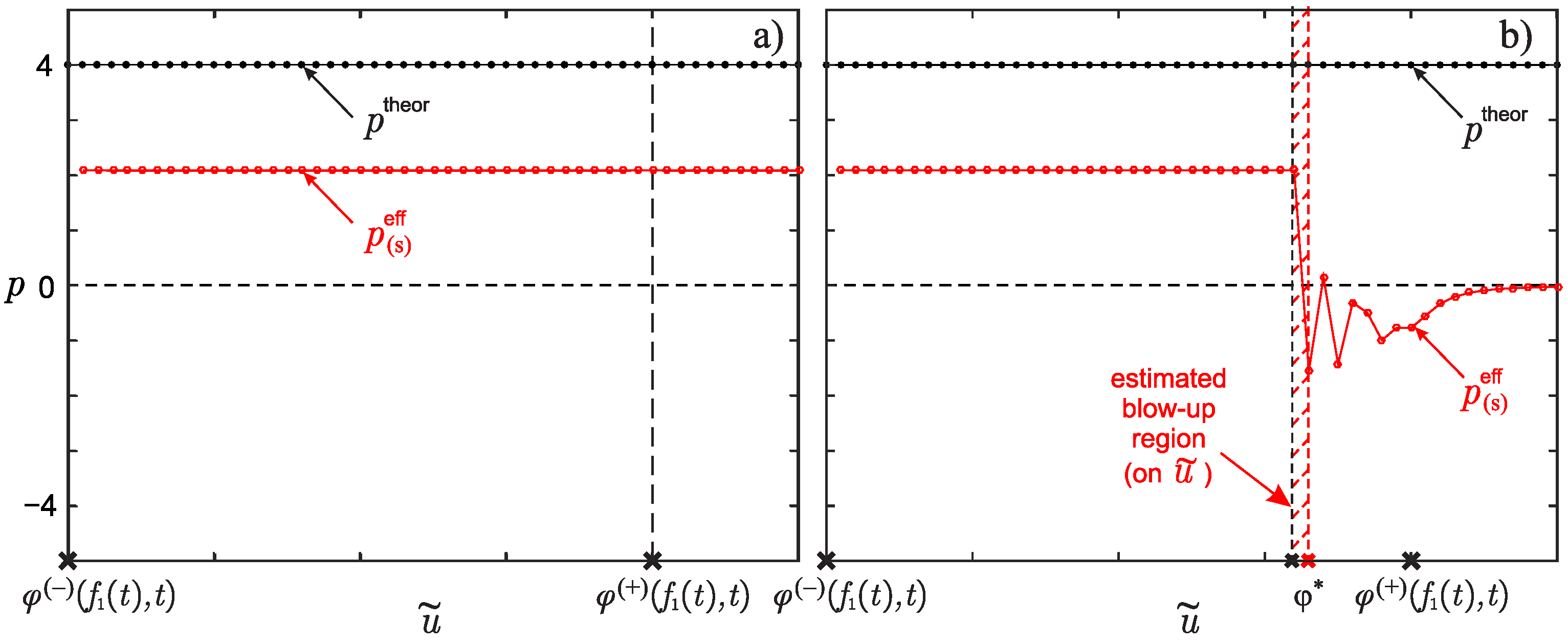
p ( s ) e f f ( u ˜ ) s p theor p .
The violation of this convergence indicates a loss of the smoothness of the exact solution on the interval u ˜ φ ( ) f 1 ( t ) , t , φ ( + ) f 1 ( t ) , t [55,56]. In particular, if p ( s ) e f f ( u ˜ ) s p e f f < 0 for some node u ˜ U ˜ , the solution does not exist globally on the domain U ˜ (see Figure 3).
Thus, the numerical algorithm for solving the problems (6) and (7) for the search for q ( t ) is formulated as follows:
  • Introduce uniform grids:
    l l T M = t m , 0 m M : t m = 0 + τ m , τ = T 0 M , U ˜ N = u ˜ n , 0 n N : u ˜ n = φ ( ) f 1 ( t ) , t + h ˜ n , h ˜ = φ ( + ) f 1 ( t ) , t φ ( ) f 1 ( t ) , t N ;
  • Smooth the function f 1 δ 1 ( t ) given by a set of grid values ( f 1 ) m f 1 δ 1 ( t m ) , m = 0 , M ¯ , using the s 3 ( t ) smoothing cubic spline. Spline s 3 minimizes functional:
    F p ( s 3 ) = p m = 0 M | ( f 1 ) m s 3 ( t m ) | 2 + ( 1 p ) m = 0 M | D 2 s 3 ( t m ) | 2 τ .
    Here, D 2 s 3 ( t ) denotes the second derivative of the function s 3 ( t ) . The smoothing parameter p can be selected based, for example, on the generalized residual principle [62]:
    m = 0 M | ( f 1 ) m s 3 p ( t m ) | 2 δ 1 2 = 0 ,
    where s 3 p is the extremal of the functional F p ( s 3 ) .
    Next, redefine ( f 1 ) m : = s 3 ( t m ) , m = 0 , M ¯ ;
  • Calculate d f 1 d t ( t m ) :
    d f 1 d t ( t m ) = 3 ( f 1 ) 0 + 4 ( f 1 ) 1 ( f 1 ) 2 2 τ , if m = 0 , ( f 1 ) m + 1 ( f 1 ) m 1 2 τ , if m = 1 , M 1 ¯ , 3 ( f 1 ) M 4 ( f 1 ) M 1 + ( f 1 ) M 2 2 τ , if m = M ;
  • For each t m T M , calculate q ( t m ) h with a given accuracy Δ using the analogue of the dichotomy method proposed above for solving the problems (6) and (7):
    (a)
    As an initial approximation, we chose h ( 0 ) and h ( 1 ) such that G ( h ( 0 ) ) G ( h ( 1 ) ) < 0 . The algorithm for calculating the auxiliary function G ( h ) is shown below;
    (b)
    Let us set the iteration number s : = 1 ;
    (c)
    Define the next approximation as h ( s + 1 ) : = h ( s ) + h ( s 1 ) 2 ;
    (d)
    If G ( h ( s + 1 ) ) G ( h ( s 1 ) ) 0 , redefine h ( s ) : = h ( s 1 ) ;
    (e)
    Redefine s : = s + 1 . If | h ( s ) h ( s 1 ) | > Δ , then go to Item 4c. Otherwise, we stop the iterative process and define h : = h ( s ) as the solution.
    The algorithm for calculating the auxiliary function G ( h ) is as follows:
    (a)
    Calculate the set of solutions v ( r s 1 N ) ( u ˜ ) of the problem (6) for the value q ˜ = h on the sequence from S grids U ˜ r s 1 N with numbers s = 1 , S ¯ using some numerical scheme with a theoretical order of accuracy p 1 ;
    (b)
    Calculate p ( S ) e f f ( u ˜ ) at the nodes of the base grid U ˜ N :
    p ( S ) e f f ( u ˜ n ) = log r | v ( r S 2 N ) ( u ˜ n ) v ( r S 3 N ) ( u ˜ n ) | | v ( r S 1 N ) ( u ˜ n ) v ( r S 2 N ) ( u ˜ n ) | , n = 1 , N ¯ ;
    (c)
    Calculate the function G ( h ) by the formula:
    G ( h ) = 1 , if p ( S ) e f f ( u ˜ n ) 1 for all n = 1 , N ¯ , 1 , if there is n 1 , N ¯ , for which p ( S ) e f f ( u ˜ n ) 0 .
    Thus, we recover the unknown function q ( t ) pointwise at each point t = t m , m = 0 , M ¯ .

2.4. Numerical Experiments

Let us consider the efficiency of the proposed algorithm by the example of solving the inverse problems (1) and (2) for the following set of model parameters:
B u , x , t , q ( t ) = u 1 u + 1 u q ( t ) , u i n i t ( x ) = tanh x 0.5 ε , T = 2 π , q ( t ) q m o d e l ( t ) = 2 30 exp 4 5 t 14 π 30 2 + 1 10 exp 1 2 t 6 π 5 2 .
For the specified set of model parameters, by solving the problem in the full statement, the function f 1 ( t ) was simulated, which was then noisy with some error δ 1 according to the following algorithm:
  • Let us solve the direct problem (1) numerically for the known q ( t ) q m o d e l ( t ) . Thus, we obtain a set of grid values of the function u ( x , t m ) , m = 0 , M ¯ , for each t m , m = 0 , M ¯ ;
  • For each value t m , find the intersection of the functions u ( x , t m ) and q m o d e l ( t m ) (see Figure 1b). This means that we have to find the root x of the following nonlinear equation:
    u ( x , t m ) q m o d e l ( t m ) = 0 .
    The found root x will be the true position f 1 ( t m ) of the moving front of the reaction at the moment of time t m ;
  • Let us introduce noise into the simulated input data of the inverse problem as follows:
    f 1 δ 1 ( t m ) = f 1 ( t m ) 1 + ξ δ 100 % ,
    where ξ —a random number uniformly distributed on the segment [ 1 , 1 ] and δ —the upper estimate of the experimental error in percent. Then, redefine δ 1 : = f 1 f 1 δ 1 L 2 .
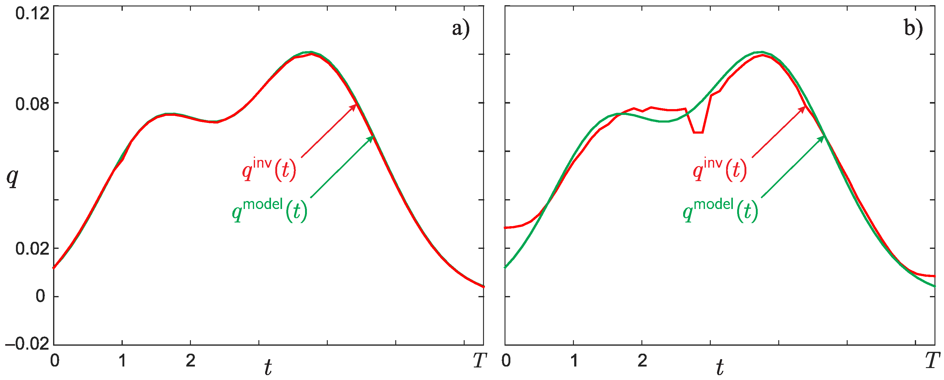
Let us first carry out calculations for the value of the singular parameter ε = 10 2 . Figure 4 shows the result of restoring the function q ( t ) q i n v ( t ) from simulated data f 1 δ 1 ( t ) set with relative errors of 0 % and 5 % . When implementing the proposed search algorithm q ( t ) , we used grids with N = 50 and M = 50 intervals, Δ = 10 6 , S = 6 .
It can be seen from the calculation results that the reconstructed function q i n v ( t ) reproduces the model function q m o d e l ( t ) rather well. This is because the singular parameter ε is small enough. Therefore, the solution q ( t ) obtained from the reduced formulation of the problem (5) can be used as a solution to the original inverse problem in the full statements (1) and (2).
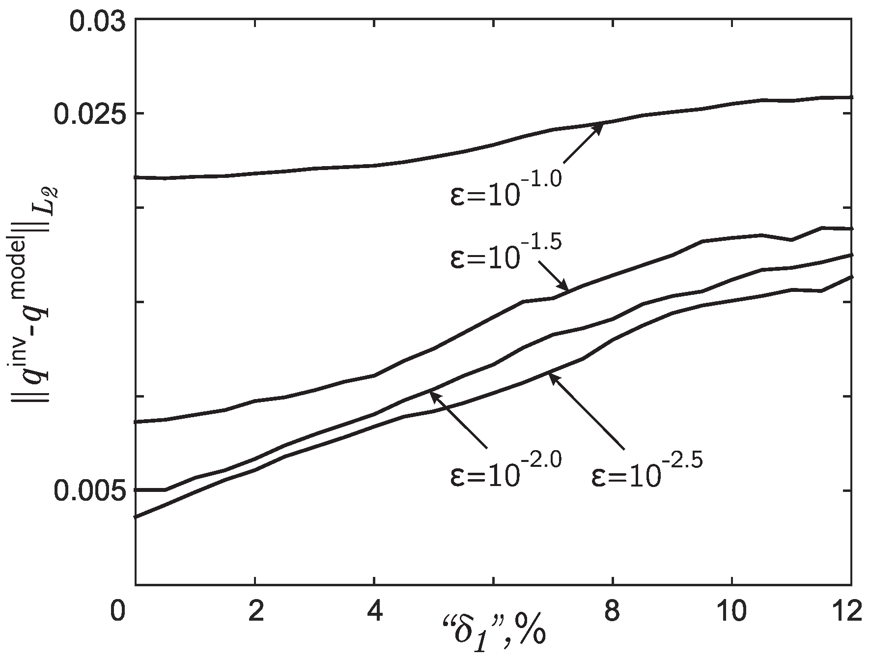
Let us investigate the question of the stability of the solution to the inverse problem depending on the level of errors in the input data δ 1 for different values of the parameter ε . For this, for different values of ε and different values of δ 1 , we found an approximate solution to the inverse problem q i n v ( t ) from the reduced formulation of the problem (5). Figure 5 shows the dependence of q i n v ( t ) q m o d e l ( t ) L 2 ( [ 0 , T ] ) on the error level input data “ δ 1 = δ 1 / < f 1 δ 1 ( t ) L 2 ( [ 0 , T ] ) > · 100 % , expressed in percent, where < · > means averaging over a set of experiments (10 pieces) for the same δ 1 . It can be seen that as δ 1 decreases, the accuracy of retrieving the function q i n v ( t ) increases. Moreover, smaller values of ε lead to a more accurate reconstruction of the required function q ( t ) .
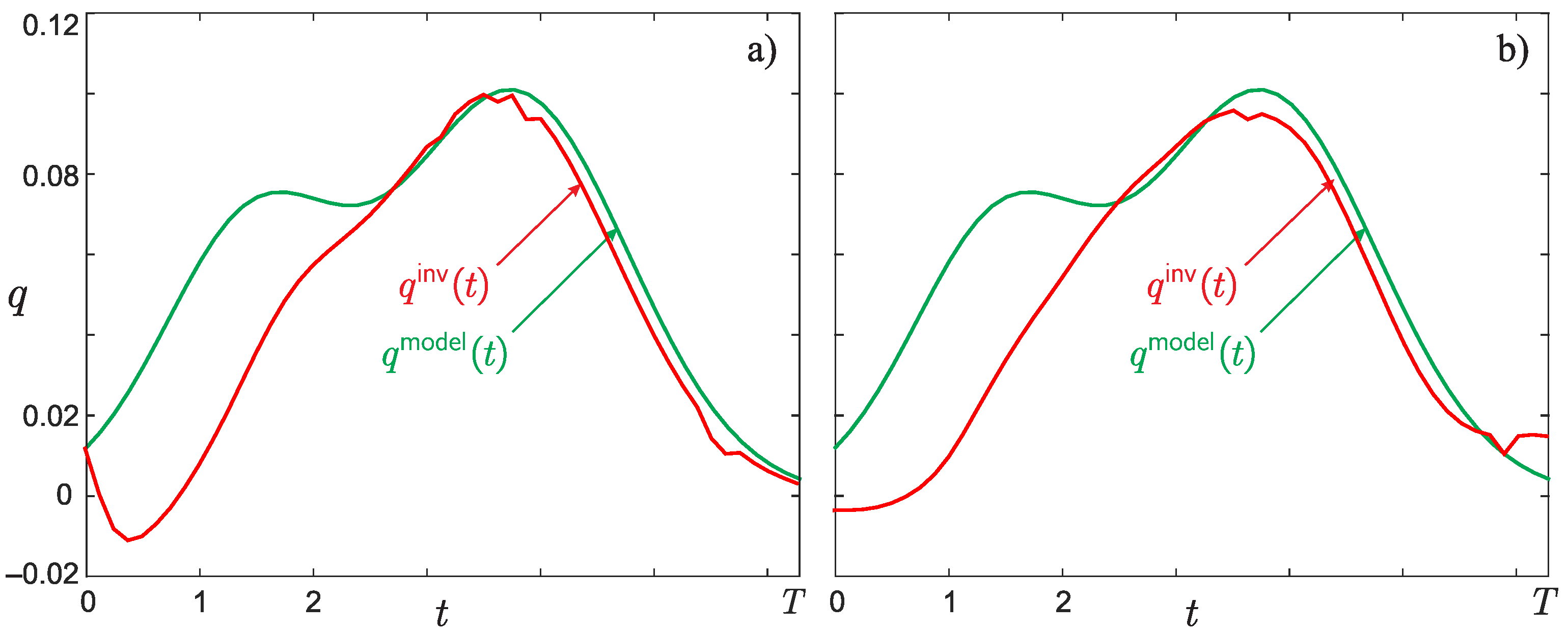
Let us demonstrate separately the calculation results for the set of model parameters (10) and the value of the singular parameter ε = 10 1 . Figure 6 shows the result of restoring the function q ( t ) from simulated data f 1 δ 1 ( t ) , specified with relative errors at the levels of 0 % and 5 % .
It can be seen from the results of the calculations that the reconstructed function q i n v ( t ) differs quite strongly from the model solution q m o d e l ( t ) both quantitatively and qualitatively (for example, the number of clearly distinguishable local extrema of functions q m o d e l ( t ) and q i n v ( t ) is different). This is due to the fact that the “small” singular parameter ε in the case of the problem under consideration for the set of parameters (10) does not satisfy the conditions of applicability of the proposed solution algorithm. In this regard, the original problem must be solved in a full statement. However, the solution obtained using the considered algorithm can be used as a good initial approximation when implementing the gradient method for minimizing the target functional when solving the problem in its full statement.

3. Modified Statement of the Inverse Problem and a Method for Its Solution Based on Minimizing the Target Functional

3.1. Full Statement of the Inverse Problem with Additional Information

Let us consider a situation in which the value of the “small” singular parameter ε in the problem (1) does not satisfy the conditions of the applicability of the methods of asymptotic analysis. In this case, we cannot search for a solution to the inverse problems (1) and (2) in the form of a solution to the reduced formulation of the problem (5). Therefore, we modified the formulation of the inverse problem considered in Section 2.1 as follows. In addition to the input information about the position of the reaction front, we require the availability of information about the value of the function u on the curve determined by the trajectory of the reaction front. This additional information makes it possible to reduce the solution of the inverse problem in its full statement to the search for a solution by the gradient method of minimizing the target functional. Thus, the inverse problem with refined input data can be formulated as follows.
The inverse problem is to determine the function q ( t ) , t [ 0 , T ] , in (1) from the known additional information about the position of the reaction front and the value of the function u at this front (see Figure 1b):
x t . p . ( t ) = f 1 ( t ) , u x t . p . ( t ) , t = f 2 ( t ) , t [ 0 , T ] .
Note that, in practice, instead of exact data f 1 ( t ) and f 2 ( t ) , their approximate values f 1 δ 1 and f 2 δ 2 are known, such that:
f 1 f 1 δ 1 L 2 δ 1 , f 2 f 2 δ 2 L 2 δ 2 .
Remark 6.
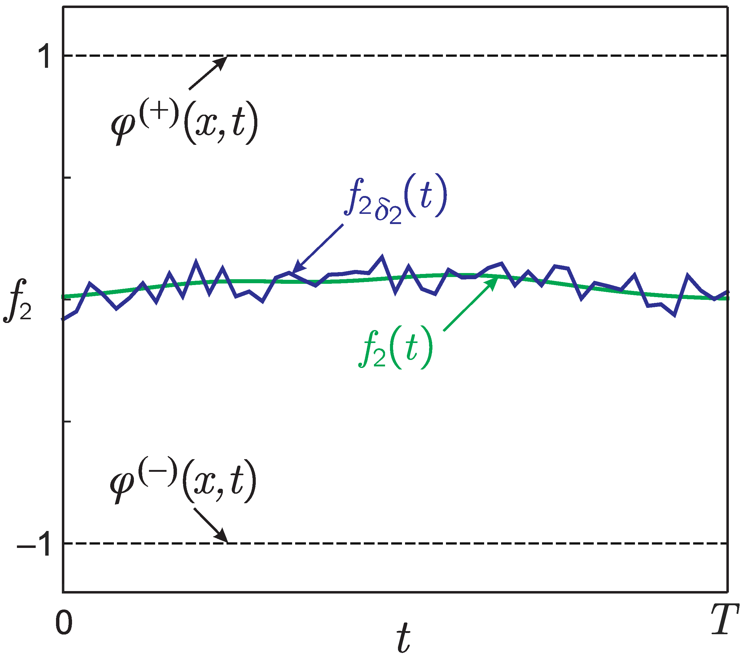
Note that according to the formal definition of the function f 2 ( t ) (see Figure 1b), one might get the impression that the required function q ( t ) can be defined in the simplest way, namely, as q ( t ) : = f 2 δ 2 ( t ) . However, taking into account possible significant errors in the experimental determination of the values of the function u ( x , t ) lying on the reaction front, such a definition of the function q ( t ) is incorrect (see Figure 7).
The algorithm proposed below makes it possible to obtain a reasonable approximation of the sought function.

3.2. Numerical Algorithm for Solving the Inverse Problem in a Full Statement

The solution to the inverse problems (1)–(11) can be found as an element q i n v ( t ) , realizing the minimum of the Tikhonov functional [62]:
J [ q ] = 0 T u f 1 ( t ) , t ; q f 2 ( t ) 2 d t + α Ω [ q ] .
Here, Ω [ q ] is a smoothing functional. In this paper, we used Ω [ q ] q W 2 2 2 :
Ω [ q ] = 0 T q 2 ( t ) + q 2 ( t ) d t .
Furthermore, in (12): u ( x , t ; q ) —the solution of the direct problem (1) for a given function q ( t ) and α —the regularization parameter, which can be chosen, for example, according to the generalized discrepancy principle.
The algorithm for the numerical solution of the inverse problem in the full statements (1)–(11), based on the minimization of the functional (12), can be implemented in the following form.
  • Let us set s : = 0 and q ( 0 ) ( t ) , t ( 0 , T ) , as the initial approximation. The function q ( 0 ) ( t ) can be any arbitrary function. A rational way of choosing it is indicated below:
  • Let us find the solution u ( s ) ( x , t ) of the direct problem:
    ε 2 2 u ( s ) x 2 ε u ( s ) t = B u ( s ) , x , t , q ( s ) ( t ) , x ( 0 , 1 ) , t ( 0 , T ] , u x ( s ) ( 0 , t ) = u x l e f t ( t ) , u x ( s ) ( 1 , t ) = u x r i g h t ( t ) , t ( 0 , T ] , u ( s ) ( x , 0 ) = u i n i t ( x ) , x [ 0 , 1 ] ;
  • Let us find the solution ψ ( s ) ( x , t ) of the adjoint problem:
    ε 2 2 ψ ( s ) x 2 + ε ψ ( s ) t = ψ ( s ) B u u ( s ) , x , t , q ( s ) ( t ) + + 2 δ x f 1 ( t ) u ( s ) ( x , t ) f 2 ( t ) , x ( 0 , 1 ) , t [ 0 , T ) , ψ x ( s ) ( 0 , t ) = 0 , ψ x ( s ) ( 1 , t ) = 0 , t [ 0 , T ) , ψ ( s ) ( x , T ) = 0 , x [ 0 , 1 ] .
    Here, δ ( x ) is the Dirac delta function;
  • Find the gradient of the functional (12):
    J q ( s ) ( t ) = 0 1 u ( s ) φ ( ) u ( s ) φ ( + ) ψ ( s ) d x + α Ω q ( s ) ( t ) .
    The derivative Ω q ( s ) ( t ) of the smoothing functional can be calculated either analytically or numerically;
  • Let us find an approximate solution at the next iteration step:
    q ( s + 1 ) ( t ) = q ( s ) ( t ) β s J q ( s ) ( t ) ,
    where β s is the descent parameter;
  • Let us check the condition for stopping the iterative process (see [36]). If it holds, we set q i n v ( t ) : = q ( s + 1 ) ( t ) as a solution to the inverse problem. Otherwise, set s : = s + 1 , and go to Step 2.
Remark 7.
When solving the inverse problem in its full statement by the gradient method described above, we cannot recover the function q ( t ) at the boundary points t = 0 and t = T .
The presence of a priori information about the desired solution allows significantly reducing the number of iterations when implementing the algorithm [63,64]. As such a priori information, we used the function q ( 0 ) ( t ) , obtained as a solution to the inverse problem in the reduced formulation (5).
Remark 8.
When calculating the gradient of the functional, the approach [65] can be used, which allows minimizing the RAM costs by almost two-times compared to the standard approach, as well as the computing resources of the processor are used in a more efficient way.

3.3. Numerical Experiments

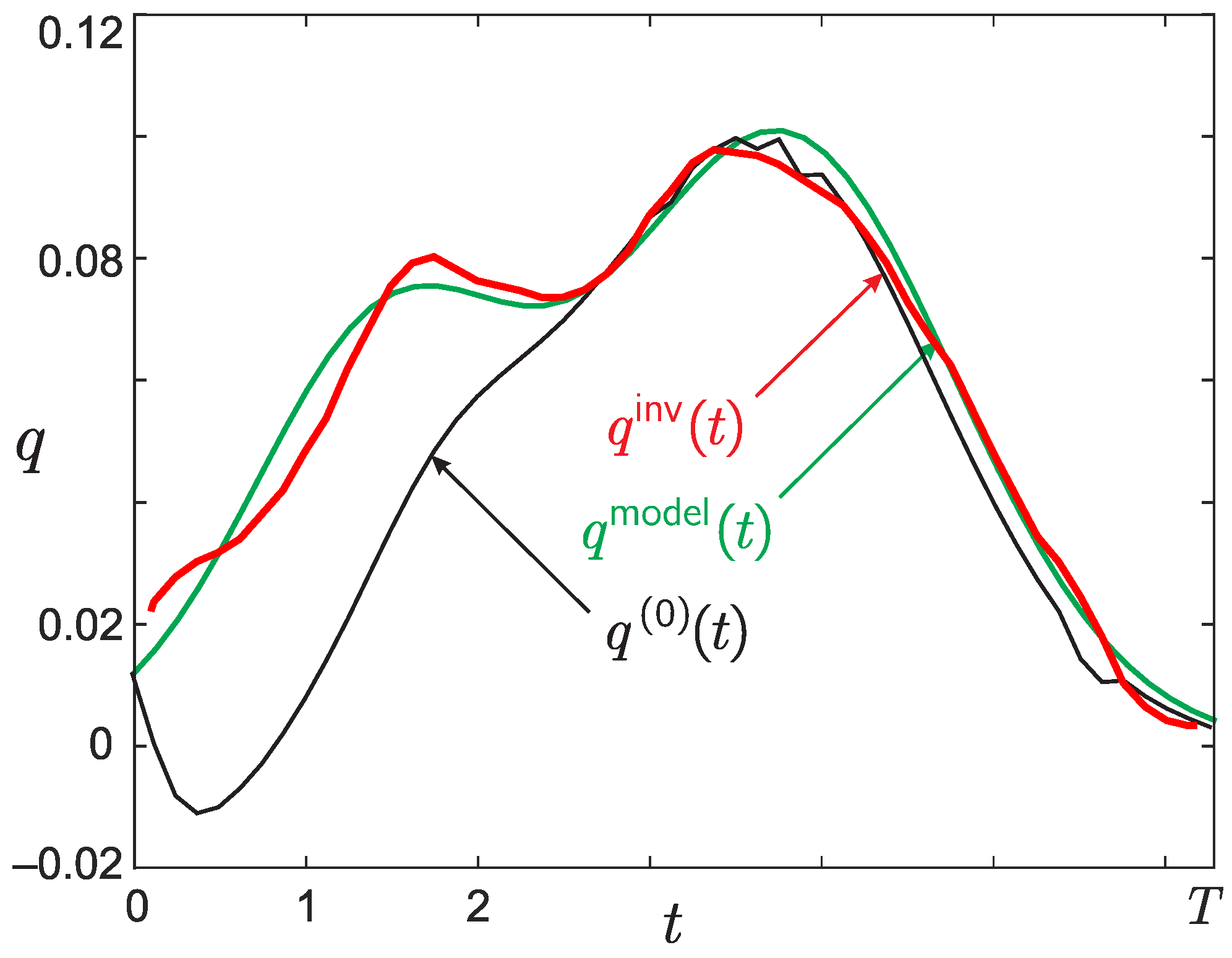
Let us consider the efficiency of the proposed algorithm, based on minimizing the target functional (12), using as an example the model set of parameters (10), ε = 10 1 , function f 1 δ 1 ( t ) with the specified noise level δ 1 = 0 % , and function f 2 δ 2 ( t ) with the specified noise level δ 2 = 75 % . As an initial approximation q ( 0 ) ( t ) , we used the solution of the problem in the reduced formulation (5). The details of the numerical implementation of the algorithm were described in [36], p. 4.
Figure 8 shows the result of restoring the function q i n v ( x ) in the case of starting with a “good” initial approximation q ( 0 ) ( t ) . The obtained solution is no longer qualitatively and quantitatively different from the true one, especially considering that it was reconstructed from the data f 2 δ 2 ( t ) given with significant errors.
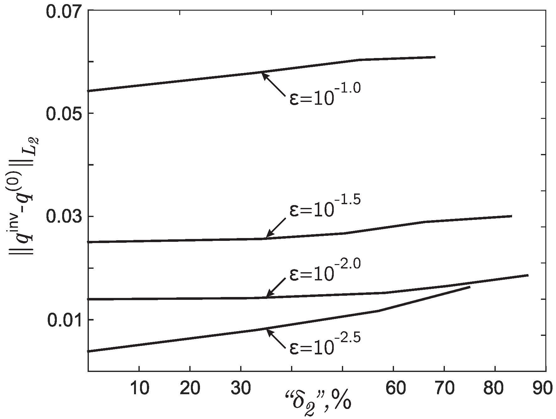
Additionally, it is possible to carry out a numerical study of the dependence q i n v q ( 0 ) L 2 on the error { δ 1 , δ 2 } for specifying the input data f 1 δ 1 and f 2 δ 2 for different values of the small parameter ε (see Figure 9).
The meaning of this dependence is the magnitude of the discrepancy between the initial approximation, chosen based on the methods of asymptotic analysis, and the solution of the inverse problem in the full statement. The smaller the value of the corresponding norm of the difference, the closer the initial approximation lies to the true solution. On the one hand, from the results obtained, it is possible to draw an additional conclusion about at what values of the singular parameter ε , the solution found from the reduced formulation of the problem is sufficiently close to the solution of the considered inverse problem in the full statement. On the other hand, we can conclude at what values of ε , the method based on the minimization of the target functional (12) makes it possible to significantly refine the initial approximation q ( 0 ) , which is only a rough approximation of the true solution.

4. Conclusions

The paper considered some features of the numerical reconstruction of an unknown coefficient in one inverse problem for an equation of the reaction–diffusion-type with data on the position of a reaction front. To solve the inverse problem, we used both (1) a method based on solving the problem in a reduced formulation obtained using the methods of asymptotic analysis and (2) a method based on minimizing the objective functional by a gradient method with the choice of an initial approximation, the search for which was based on the use of the methods of asymptotic analysis. It was shown that under certain conditions, the gradient method can significantly refine the a priori information about the solution obtained by the methods of asymptotic analysis. However, based on the results of the study, it is necessary to make the following remarks:
  • When constructing a “good” initial approximation q ( 0 ) ( t ) using the proposed algorithm, the error determining the difference between this approximation and the true solution was estimated only numerically. The question of the possibility of performing rigorous analytical estimates remains open and is of significant interest as a topic for a separate work;
  • The question of strict conditions under which a “good” initial approximation is guaranteed to lie in the vicinity of the global minimum of the objective functional is open. The corresponding question is also of significant interest and may be the topic of a separate work devoted to the properties of global convergence [66,67,68,69,70]. Note that a globally converging algorithm means an algorithm that allows one to find the global minimum regardless of the choice of the initial approximation. In the event that a “good” initial approximation, chosen automatically using the proposed algorithm, lies in the vicinity of a global minimum, the algorithm will have the properties of global convergence;
  • As prospects for the development of the proposed method, the implementation of methods for performing a posteriori estimation of the accuracy of the obtained solution should be noted (see, for example, [71,72,73,74,75,76,77,78,79,80,81]).

Author Contributions

Conceptualization, D.L.; methodology, D.L., R.A., A.G. and M.S.; software, A.G. and R.A.; validation, A.G. and R.A.; formal analysis, D.L. and M.S.; investigation, D.L. and R.A.; resources, A.G.; data curation, R.A.; writing—original draft preparation, D.L.; writing—review and editing, D.L.; visualization, D.L. and R.A.; supervision, D.L.; project administration, D.L.; funding acquisition, D.L. All authors have read and agreed to the published version of the manuscript.

Funding

The reported study was funded by RFBR, Project Number 20-31-70016.

Institutional Review Board Statement

Not applicable.

Informed Consent Statement

Not applicable.

Acknowledgments

The paper was published with the support of the Ministry of Education and Science of the Russian Federation as part of the program of the Moscow Center for Fundamental and Applied Mathematics under Agreement N075-15-2019-1621.

Conflicts of Interest

The authors declare no conflict of interest.

References

  1. Danilov, V.; Maslov, V.; Volosov, K. Mathematical Modelling of Heat and Mass Transfer Processes; Kluwer: Dordrecht, The Netherlands, 1995. [Google Scholar]
  2. Zeldovich, Y.; Barenblatt, G.; Librovich, V.; Makhviladze, G. The Mathematical Theory of Combustion and Explosions; Plenum: New York, NY, USA, 1985. [Google Scholar]
  3. Butuzov, V.; Vasil’eva, A. Singularly perturbed problems with boundary and interior layers: Theory and applications. Adv. Chem. Phys. 1997, 97, 47–179. [Google Scholar]
  4. Liu, Z.; Liu, Q.; Lin, H.C.; Schwartz, C.; Lee, Y.H.; Wang, T. Three-dimensional variational assimilation of MODIS aerosol optical depth: Implementation and application to a dust storm over East Asia. J. Geophys. Res. Atmos. 2010, 116, D23206. [Google Scholar] [CrossRef] [Green Version]
  5. Egger, H.; Fellner, K.; Pietschmann, J.F.; Tang, B.Q. Analysis and numerical solution of coupled volume-surface reaction–diffusion systems with application to cell biology. Appl. Math. Comput. 2018, 336, 351–367. [Google Scholar] [CrossRef] [Green Version]
  6. Yaparova, N. Method for determining particle growth dynamics in a two-component alloy. Steel Transl. 2020, 50, 95–99. [Google Scholar] [CrossRef]
  7. Lin, G.; Zhang, Y.; Cheng, X.; Gulliksson, M.; Forssén, P.; Fornstedt, T. A regularizing Kohn—Vogelius formulation for the model-free adsorption isotherm estimation problem in chromatography. Appl. Anal. 2018, 97, 13–40. [Google Scholar] [CrossRef]
  8. Wu, X.; Ni, M. Existence and stability of periodic contrast structure in reaction-advection-diffusion equation with discontinuous reactive and convective terms. Commun. Nonlinear Sci. Numer. Simul. 2020, 91, 105457. [Google Scholar] [CrossRef]
  9. Zhang, Y.; Lin, G.; Gulliksson, M.; Forssén, P.; Fornstedt, T.; Cheng, X. An adjoint method in inverse problems of chromatography. Inverse Probl. Sci. Eng. 2017, 25, 1112–1137. [Google Scholar] [CrossRef]
  10. Volpert, A.; Volpert, V.; Volpert, V. Traveling Wave Solutions of Parabolic Systems; American Mathematical Society: Providence, RI, USA, 2000. [Google Scholar]
  11. Meinhardt, H. Models of Biological Pattern Formation; Academic Press: London, UK, 1982. [Google Scholar]
  12. FitzHugh, R. Impulses and physiological states in theoretical model of nerve membrane. Biophys. J. 1961, 1, 445–466. [Google Scholar] [CrossRef] [Green Version]
  13. Murray, J. Mathematical Biology. I. An Introduction; Springer: New York, NY, USA, 2002. [Google Scholar] [CrossRef]
  14. Egger, H.; Pietschmann, J.F.; Schlottbom, M. Identification of nonlinear heat conduction laws. J. Inverse-Ill Probl. 2015, 23, 429–437. [Google Scholar] [CrossRef] [Green Version]
  15. Gholami, A.; Mang, A.; Biros, G. An inverse problem formulation for parameter estimation of a reaction–diffusion model of low grade gliomas. J. Math. Biol. 2016, 72, 409–433. [Google Scholar] [CrossRef] [PubMed] [Green Version]
  16. Aliev, R.; Panfilov, A. A simple two-variable model of cardiac excitation. Chaos Solitons Fractals 1996, 7, 293–301. [Google Scholar] [CrossRef]
  17. Generalov, E.; Levashova, N.; Sidorova, A.; Chumankov, P.; Yakovenko, L. An autowave model of the bifurcation behavior of transformed cells in response to polysaccharide. Biophysics 2017, 62, 876–881. [Google Scholar] [CrossRef]
  18. Mang, A.; Gholami, A.; Davatzikos, C.; Biros, G. PDE-constrained optimization in medical image analysis. Optim. Eng. 2018, 19, 765–812. [Google Scholar] [CrossRef] [Green Version]
  19. Kabanikhin, S.; Shishlenin, M. Recovering a Time-Dependent Diffusion Coefficient from Nonlocal Data. Numer. Anal. Appl. 2018, 11, 38–44. [Google Scholar] [CrossRef]
  20. Mamkin, V.; Kurbatova, J.; Avilov, V.; Mukhartova, Y.; Krupenko, A.; Ivanov, D.; Levashova, N.; Olchev, A. Changes in net ecosystem exchange of CO2, latent and sensible heat fluxes in a recently clear-cut spruce forest in western Russia: Results from an experimental and modeling analysis. Environ. Res. Lett. 2016, 11, 125012. [Google Scholar] [CrossRef]
  21. Levashova, N.; Muhartova, J.; Olchev, A. Two approaches to describe the turbulent exchange within the atmospheric surface layer. Math. Model. Comput. Simul. 2017, 9, 697. [Google Scholar] [CrossRef]
  22. Levashova, N.; Sidorova, A.; Semina, A.; Ni, M. A spatio-temporal autowave model of shanghai territory development. Sustainability 2019, 11, 3658. [Google Scholar] [CrossRef] [Green Version]
  23. Isakov, V.; Kabanikhin, S.; Shananin, A.; Shishlenin, M.; Zhang, S. Algorithm for determining the volatility function in the Black-Scholes model. Comput. Math. Math. Phys. 2019, 59, 1753–1758. [Google Scholar] [CrossRef]
  24. Kadalbajoo, M.; Gupta, V. A brief survey on numerical methods for solving singularly perturbed problems. Appl. Math. Comput. 2010, 217, 3641–3716. [Google Scholar] [CrossRef]
  25. Kabanikhin, S. Definitions and examples of inverse and ill-posed problems. J. Inverse-Ill Probl. 2008, 16, 317–357. [Google Scholar] [CrossRef]
  26. Kabanikhin, S. Inverse and Ill-Posed Problems Theory and Applications; De Gruyter: Berlin, Germany, 2011. [Google Scholar]
  27. Jin, B.; Rundell, W. A tutorial on inverse problems for anomalous diffusion processes. Inverse Probl. 2015, 31, 035003. [Google Scholar] [CrossRef] [Green Version]
  28. Belonosov, A.; Shishlenin, M. Regularization methods of the continuation problem for the parabolic equation. Lect. Notes Comput. Sci. 2017, 10187, 220–226. [Google Scholar]
  29. Kaltenbacher, B.; Rundell, W. On the identification of a nonlinear term in a reaction–diffusion equation. Inverse Probl. 2019, 35, 115007. [Google Scholar] [CrossRef] [Green Version]
  30. Belonosov, A.; Shishlenin, M.; Klyuchinskiy, D. A comparative analysis of numerical methods of solving the continuation problem for 1D parabolic equation with the data given on the part of the boundary. Adv. Comput. Math. 2019, 45, 735–755. [Google Scholar] [CrossRef]
  31. Kaltenbacher, B.; Rundell, W. The inverse problem of reconstructing reaction–diffusion systems. Inverse Probl. 2020, 36, 065011. [Google Scholar] [CrossRef]
  32. Kumarasamy, S.; Soundararajan, G.; Natesan, B.B.; Balachandran, K. Inverse problem for the reaction diffusion system by optimization method. Appl. Math. Model. 2011, 35, 571–579. [Google Scholar] [CrossRef]
  33. Tatar, S.; Ulusoy, S. An inverse coefficient problem for a nonlinear reaction diffusion equation with a nonlinear source. Electron. J. Differ. Equ. 2015, 245, 2015. [Google Scholar]
  34. Kaltenbacher, B.; Rundell, W. Recovery of multiple coefficients in a reaction–diffusion equation. J. Math. Anal. Appl. 2019, 481, 123475. [Google Scholar] [CrossRef]
  35. Cristofol, M.; Roques, L. An inverse problem involving two coefficients in a nonlinear reaction–diffusion equation. Comptes Rendus Math. 2012, 350, 469–473. [Google Scholar] [CrossRef] [Green Version]
  36. Lukyanenko, D.; Borzunov, A.; Shishlenin, M. Solving coefficient inverse problems for nonlinear singularly perturbed equations of the reaction-diffusion-advection-type with data on the position of a reaction front. Commun. Nonlinear Sci. Numer. Simul. 2021, 99, 105824. [Google Scholar] [CrossRef]
  37. Lukyanenko, D.; Yeleskina, T.; Prigorniy, I.; Isaev, T.; Borzunov, A.; Shishlenin, M. Inverse problem of recovering the initial condition for a nonlinear equation of the reaction-diffusion-advection-type by data given on the position of a reaction front with a time delay. Mathematics 2021, 9, 342. [Google Scholar] [CrossRef]
  38. Zakharova, S.; Davydova, M.; Lukyanenko, D. Use of asymptotic analysis for solving the inverse problem of source parameters determination of nitrogen oxide emission in the atmosphere. Inverse Probl. Sci. Eng. 2021, 29, 365–377. [Google Scholar] [CrossRef]
  39. Lukyanenko, D.; Prigorniy, I.; Shishlenin, M. Some features of solving an inverse backward problem for a generalized Burgers’ equation. J. Inverse-Ill Probl. 2020, 28, 641–649. [Google Scholar] [CrossRef]
  40. Levashova, N.; Gorbachev, A.; Argun, R.; Lukyanenko, D. The problem of the non-uniqueness of the solution to the inverse problem of recovering the symmetric states of a bistable medium with data on the position of an autowave front. Symmetry 2021, 13, 860. [Google Scholar] [CrossRef]
  41. Argun, R.; Gorbachev, A.; Levashova, N.; Lukyanenko, D. Inverse problem for an equation of the reaction–diffusion–advection type with data on the position of a reaction front: Features of the solution in the case of a nonlinear integral equation in a reduced statement. Mathematics 2021, 9, 2342. [Google Scholar] [CrossRef]
  42. Vasil’eva, A.; Butuzov, V.; Nefedov, N. Singularly perturbed problems with boundary and internal layers. Proc. Steklov Inst. Math. 2010, 268, 258–273. [Google Scholar] [CrossRef]
  43. Henkin, G.M.; Shananin, A.A.; Tumanov, A.T. Estimates for solutions of Burgers type equations and some applications. J. Math. Pures Appl. 2004, 84, 717–752. [Google Scholar] [CrossRef] [Green Version]
  44. Henkin, G.M. Asymptotic structure for solutions of the Cauchy problem for Burgers type equations. J. Fixed Point Theory Appl. 2007, 1, 239–291. [Google Scholar] [CrossRef]
  45. Mitidieri, E.; Pohozaev, S. A Priori Estimates and Blow-Up of Solutions to Nonlinear Partial Differential Equations and Inequalities; Trudy Mat. Inst. Steklova: Moscow, Russia, 2001; Volume 234, pp. 3–383. [Google Scholar]
  46. Levine, H.A. Some nonexistence and instability theorems for solutions of formally parabolic equations of the form Put = −Au + F(u). Arch. Ration. Mech. Anal. 1973, 51, 371–386. [Google Scholar] [CrossRef]
  47. Kalantarov, V.K.; Ladyzhenskaya, O.A. The occurrence of collapse for quasilinear equations of parabolic and hyperbolic types. Nauch. Semin. Leningr. Otd. Mat. Inst. Steklova 1977, 69, 77–102. [Google Scholar] [CrossRef]
  48. Sveshnikov, A.G.; Al’shin, A.B.; Korpusov, M.O.; Pletner, Y.D. Linear and Nonlinear Equations of Sobolev Type; Fizmatlit: Moscow, Russia, 2007. [Google Scholar]
  49. Samarskii, A.A.; Galaktionov, V.A.; Kurdyumov, S.P.; Mikhailov, A.P. Blow-Up in Quasilinear Wave Equations; Nauka: Moscow, Russia, 1987. [Google Scholar]
  50. Galaktionov, V.; Pohozaev, S. Third-order nonlinear dispersive equations: Shocks, rarefaction, and blowup waves. Comput. Math. Math. Phys. 2008, 48, 1784–1810. [Google Scholar] [CrossRef]
  51. Pelinovsky, D.; Xu, C. On numerical modelling and the blow-up behavior of contact lines with a 180 degrees contact angle. J. Eng. Math. 2015, 92, 31–44. [Google Scholar] [CrossRef]
  52. Cangiani, A.; Georgoulis, E.; Kyza, I.; Metcalfe, S. Adaptivity and blow-up detection for nonlinear evolution problems. SIAM J. Sci. Comput. 2015, 38, A3833–A3856. [Google Scholar] [CrossRef] [Green Version]
  53. Haynes, R.; Turner, C. A numerical and theoretical study of blow-up for a system of ordinary differential equations using the Sundman transformation. Atl. Electron. J. Math. 2007, 2, 1–13. [Google Scholar]
  54. Kohn, R.; Berger, M. A rescaling algorithm for the numerical calculation of blowing-up solutions. Commun. Pure Appl. Math. 1988, 41, 841–863. [Google Scholar]
  55. Alshin, A.; Kalitkin, N.; Koryakin, P. Diagnostics of singularities of exact solutions in computations with error control. Comput. Math. Math. Phys. 2005, 45, 1769–1779. [Google Scholar]
  56. Alshin, A.; Alshina, E. Numerical diagnosis of blow-up of solutions of pseudoparabolic equations. J. Math. Sci. 2008, 148, 143–162. [Google Scholar] [CrossRef]
  57. Hoffman, J.; Johnson, C. Blow up of incompressible Euler solutions. BIT Numer. Math. 2008, 48, 285–307. [Google Scholar] [CrossRef] [Green Version]
  58. Nefedov, N.; Bozhevolnov, U. Asymptotics of the front motion in the reaction–diffusion–advection problem. Comput. Math. Math. Phys. 2010, 50, 264–273. [Google Scholar]
  59. Korpusov, M.; Lukyanenko, D.; Panin, A.; Yushkov, E. Blow-up for one Sobolev problem: Theoretical approach and numerical analysis. J. Math. Anal. Appl. 2016, 442, 451–468. [Google Scholar] [CrossRef]
  60. Korpusov, M.; Lukyanenko, D.; Panin, A. Blow-up for Joseph-Egri equation: Theoretical approach and numerical analysis. Math. Methods Appl. Sci. 2020, 43, 6771–6800. [Google Scholar] [CrossRef]
  61. Korpusov, M.; Lukyanenko, D.; Panin, A.; Shlyapugin, G. On the blow-up phenomena for a 1-dimensional equation of ion sound waves in a plasma: Analytical and numerical investigation. Math. Methods Appl. Sci. 2018, 41, 2906–2929. [Google Scholar] [CrossRef]
  62. Tikhonov, A.N.; Goncharsky, A.V.; Stepanov, V.V.; Yagola, A.G. Numerical Methods for the Solution of Ill-Posed Problems; Kluwer Academic Publishers: Dordrecht, The Netherlands, 1995. [Google Scholar]
  63. Isakov, V. Inverse Problems for Partial Differential Equations; Springer: New York, NY, USA, 2006. [Google Scholar]
  64. Kabanikhin, S.; Shishlenin, M. Quasi-solution in inverse coefficient problems. J. Inverse-Ill Probl. 2008, 16, 705–713. [Google Scholar] [CrossRef]
  65. Klyuchinskiy, D.; Novikov, N.; Shishlenin, M. CPU-time and RAM memory optimization for solving dynamic inverse problems using gradient-based approach. J. Comput. Phys. 2021, 439, 110374. [Google Scholar] [CrossRef]
  66. Klibanov, M.; Li, J.; Zhang, W. Convexification for an inverse parabolic problem. Inverse Probl. 2020, 36, 085008. [Google Scholar] [CrossRef]
  67. Klibanov, M.; Nguyen, D.L. Convergence of a series associated with the convexification method for coefficient inverse problems. J. Inverse-Ill Probl. 2020, 29. [Google Scholar] [CrossRef]
  68. Bakushinskii, A.; Kokurin, M.; Kokurin, M. Direct and Converse Theorems for Iterative Methods of Solving Irregular Operator Equations and Finite Difference Methods for Solving Ill-Posed Cauchy Problems. Comput. Math. Math. Phys. 2020, 60, 915–937. [Google Scholar] [CrossRef]
  69. Egger, H.; Engl, H.; Klibanov, M. Global uniqueness and Holder stability for recovering a nonlinear source term in a parabolic equation. Inverse Probl. 2005, 21, 271–290. [Google Scholar] [CrossRef]
  70. Klibanov, M.; Kamburg, V. Globally strictly convex cost functional for an inverse parabolic problem. Math. Meth. Appl. Sci. 2015, 39, 930–940. [Google Scholar] [CrossRef] [Green Version]
  71. Yagola, A.; Leonov, A.; Titarenko, V. Data errors and an error estimation for ill-posed problems. Inverse Probl. Eng. 2002, 10, 117–129. [Google Scholar] [CrossRef]
  72. Titarenko, V.; Yagola, A. Error estimation for ill-posed problems on piecewise convex functions and sourcewise represented sets. J. Inverse-Ill Probl. 2008, 16, 625–638. [Google Scholar] [CrossRef]
  73. Leonov, A. Which of inverse problems can have a priori approximate solution accuracy estimates comparable in order with the data accuracy. Numer. Anal. Appl. 2014, 7, 284–292. [Google Scholar] [CrossRef]
  74. Leonov, A. A posteriori accuracy estimations of solutions to ill-posed inverse problems and extra-optimal regularizing algorithms for their solution. Numer. Anal. Appl. 2012, 5, 68–83. [Google Scholar] [CrossRef]
  75. Kokurin, M. Accuracy estimates of regularization methods and conditional well-posedness of nonlinear optimization problems. J. Inverse-Ill Probl. 2018, 26, 789–797. [Google Scholar] [CrossRef]
  76. Kokurin, M. Ill-Posed Nonlinear Optimization Problems and Uniform Accuracy Estimates of Regularization Methods. Numer. Funct. Anal. Optim. 2020, 41, 1887–1900. [Google Scholar] [CrossRef]
  77. Zhang, Y.; Gong, R. Second order asymptotical regularization methods for inverse problems in partial differential equations. J. Comput. Appl. Math. 2020, 375. [Google Scholar] [CrossRef] [Green Version]
  78. Lin, G.; Cheng, X.; Zhang, Y. A parametric level set based collage method for an inverse problem in elliptic partial differential equations. J. Comput. Appl. Math. 2018, 340, 101–121. [Google Scholar] [CrossRef] [Green Version]
  79. Gulliksson, M.; Holmbom, A.; Persson, J.; Zhang, Y. A separating oscillation method of recovering the G-limit in standard and non-standard homogenization problems. Inverse Probl. 2016, 32, 025005. [Google Scholar] [CrossRef]
  80. Klibanov, M.; Li, J.; Zhang, W. Linear lavrent’ev integral equation for the numerical solution of a nonlinear coefficient inverse problem. SIAM J. Appl. Math. 2021, 81, 1954–1978. [Google Scholar] [CrossRef]
  81. Chaikovskii, D.; Zhang, Y. Convergence analysis for forward and inverse problems in singularly perturbed time-dependent reaction-advection-diffusion equations. arXiv 2021, arXiv:2106.15249. [Google Scholar]
Figure 1. Typical form of a solution of a moving-front-type in Problem (1) at a fixed time t. (a) The physical meaning of the value x t . p . ( t ) ; (b) the formal definition of the value of x t . p . ( t ) when applying the methods of asymptotic analysis (see Section 2.2) or the gradient method for minimizing the target functional (see Section 3.1).
Mathematics 09 02894 g001
Figure 2. An example of typical solutions to the Cauchy problem (6), obtained numerically for various values of the parameter q ˜ . Pictures correspond to the calculation of an approximate solution v ( 2 S 1 N ) ( u ˜ ) of the Cauchy problem (6) according to the ERK4 scheme with N = 50 and S = 6 for parameters φ ( ) 1 , φ ( + ) 1 , d f d t = 0.1231 , and (a) q ˜ = 0.0025 , (b) q ˜ = 0.09 . For both cases, the exact value of q is q = 0.085 .
Mathematics 09 02894 g002
Figure 3. Typical form of the functions p ( s ) e f f ( u ˜ ) , which correspond to the solutions of the Cauchy problems shown in Figure 2. Subfigures (a,b) correspond to the subfigures in Figure 2.
Mathematics 09 02894 g003
Figure 4. Exact model solution (function q m o d e l ( t ) ) and the result of its reconstruction (function q i n v ( t ) ) from the input data of the inverse problem defined by function f 1 δ 1 ( t ) simulated for a set of model parameters (10) and ε = 10 2 with error (a) δ 1 = 0 (matches δ = 0 % ) and (b) δ 1 3.5 × 10 2 (matches δ = 5 % ).
Mathematics 09 02894 g004
Figure 5. The norm of the residual q i n v ( t ) q m o d e l ( t ) L 2 ( [ 0 , T ] ) versus the noise level “ δ 1 ” of the inverse problem data for various ε .
Mathematics 09 02894 g005
Figure 6. Exact model solution (function q m o d e l ( t ) ) and the result of its reconstruction (function q i n v ( t ) ) from the input data of the inverse problem defined by function f 1 δ 1 ( t ) simulated for a set of model parameters (10) and ε = 10 1 with error (a) δ 1 = 0 (matches δ = 0 % ) and (b) δ 1 3.5 × 10 2 (matches δ = 5 % ).
Mathematics 09 02894 g006
Figure 7. Typical form of the function f 2 δ 2 ( t ) , determined in the experiment, in comparison with f 2 ( t ) . The figure shows the simulation result for a set of model parameters (10), ε = 10 1 , with errors δ 1 = 0 and δ 2 7.15 × 10 2 (matches δ 1 = 0 % and δ 2 = 75 % ).
Mathematics 09 02894 g007
Figure 8. Result of restoring the function q i n v ( x ) using the gradient method of minimizing the target functional (12). The functions f 1 δ 1 ( t ) and f 2 δ 2 ( t ) , simulated for a set of model parameters (10), ε = 10 1 , and errors { δ 1 , δ 2 } = { 0 , 7.15 × 10 2 } (matches δ 1 = 0 % and δ 2 = 75 % ). The gradient method was started with a “good” initial approximation q ( 0 ) ( t ) , which coincides in the case of the selected errors with those shown in Figure 6a.
Mathematics 09 02894 g008
Figure 9. The norm of the residual q i n v q ( 0 ) L 2 versus the noise level “ δ 2 ” of the inverse problem data for various ε (“ δ 1 = 0 % ).
Mathematics 09 02894 g009
Publisher’s Note: MDPI stays neutral with regard to jurisdictional claims in published maps and institutional affiliations.