An Extended Car-Following Model Based on Visual Angle and Electronic Throttle Effect

Abstract

With the continuous advancement of electronic technology, auto parts manufacturing institutions are gradually applying electronic throttles to automobiles for precise control. Based on the visual angle model (VAM), a car-following model considering the electronic throttle angle of the preceding vehicle is proposed. The stability conditions are obtained through linear stability analysis. By means of nonlinear analysis, the time-dependent Ginzburg–Landau (TDGL) equation is derived first, and then the modified Korteweg-de-Vries (mKdV) equation is derived. The relationship between the two is thus obtained. Finally, in the process of numerical simulations and exploration, it is shown how the visual angle and electronic throttle affect the stability of traffic flow. The simulation results in MATLAB software verify the validity of the model, indicating that the visual angle and electronic throttle can improve traffic stability.

1. Introduction

Urban roads are an important link between the city’s economy and development, and the stable operation of road traffic has an important impact on the city’s construction. Nowadays, the increasing number of motor vehicles has seriously affected the driving environment, and traffic phenomena (such as traffic congestion, road overload, average speed drop, etc.) cannot be ignored. It requires a systematic view to guide the operation of traffic flow in order to integrate vehicles, road facilities and users into a whole and facilitate collaboration. The application of traffic flow theory can better analyze the traffic phenomenon and its essence, so that the road can maximize its effectiveness. The macroscopic model, mesoscopic model, and microscopic model are the general classification of the traffic flow model, including cellular automation models [1,2,3,4], car-following models [5,6,7,8,9,10,11,12,13,14,15,16], hydrodynamic lattice models [17,18,19,20,21,22,23,24,25], continuum models [26,27,28,29,30,31,32] and route optimization models [33,34,35]. Usually, the actual traffic flow is affected by the stimulation of time and space, and its change process is a dynamic and very complicated process. Therefore, in combination with practice, the basic idea of the generalized car-following theory is “response = sensitivity × stimulus”.

According to the stimulation framework, the driver’s response comes from the stimulus given by the environment. Different variants of the car following models that provide different stimuli for the driver in the traffic flow model are shown below. The Gazis–Herman–Rothery (GHR) model [36] is based on the “response = sensitivity × stimulus” framework, which is set under the assumption that the current driver is stimulated and the acceleration of the responsively controlled vehicle is affected by the current velocity, headway and velocity difference from the previous vehicle. Its formulation is as follows:

$$\frac{d{v}_n\left(t\right)}{dt}=\lambda \Delta v_n\left(t-\tau \right)$$

(1)

where the velocity of the $n$-th car at time $t$ is represented by $v_n\left(t\right)$, the reaction time of the driver is expressed as $\tau$, the sensitivity of the relative speed is expressed as $\lambda$, and the relative speed of time $t-\tau$ is expressed as $\Delta v_n\left(t-\tau \right)$.

The optimal velocity model (OVM for short) is proposed by Bando et al. [37]. They took the optimal velocity of driver into account. The OVM model formula is as follows:

$$\frac{d{v}_n\left(t\right)}{dt}=\alpha \left[V\left(\Delta x_n\left(t\right)\right)-v_n\left(t\right)\right]$$

(2)

where the sensitivity of a driver is represented by $\alpha$, the optimal velocity function is represented by $V\left(\Delta x_n\left(t\right)\right)$, and the difference in headway of two successive vehicles is represented by $\Delta x_n\left(t\right)=x_{n+1}\left(t\right)-x_n\left(t\right)$.

The acceleration in OVM is too high and the deceleration is impractical; therefore, Helbing et al. [38] put forward the generalized force model (GFM). GFM has two drawbacks under blocking density, one of which is that it cannot account for the delay time of the vehicle motion, and the other is that it cannot describe the velocity of kinematic wave speed. Jiang et al. [39,40] believed that only considering the impact of negative velocity difference on cars is still inadequate, so they developed the full velocity difference model (FVD). Its formula is as follows:

$$\frac{d{v}_n\left(t\right)}{dt}=\alpha \left[V\left(\Delta x_n\left(t\right)\right)-v_n\left(t\right)\right]+\lambda \Delta v_n\left(t\right)$$

(3)

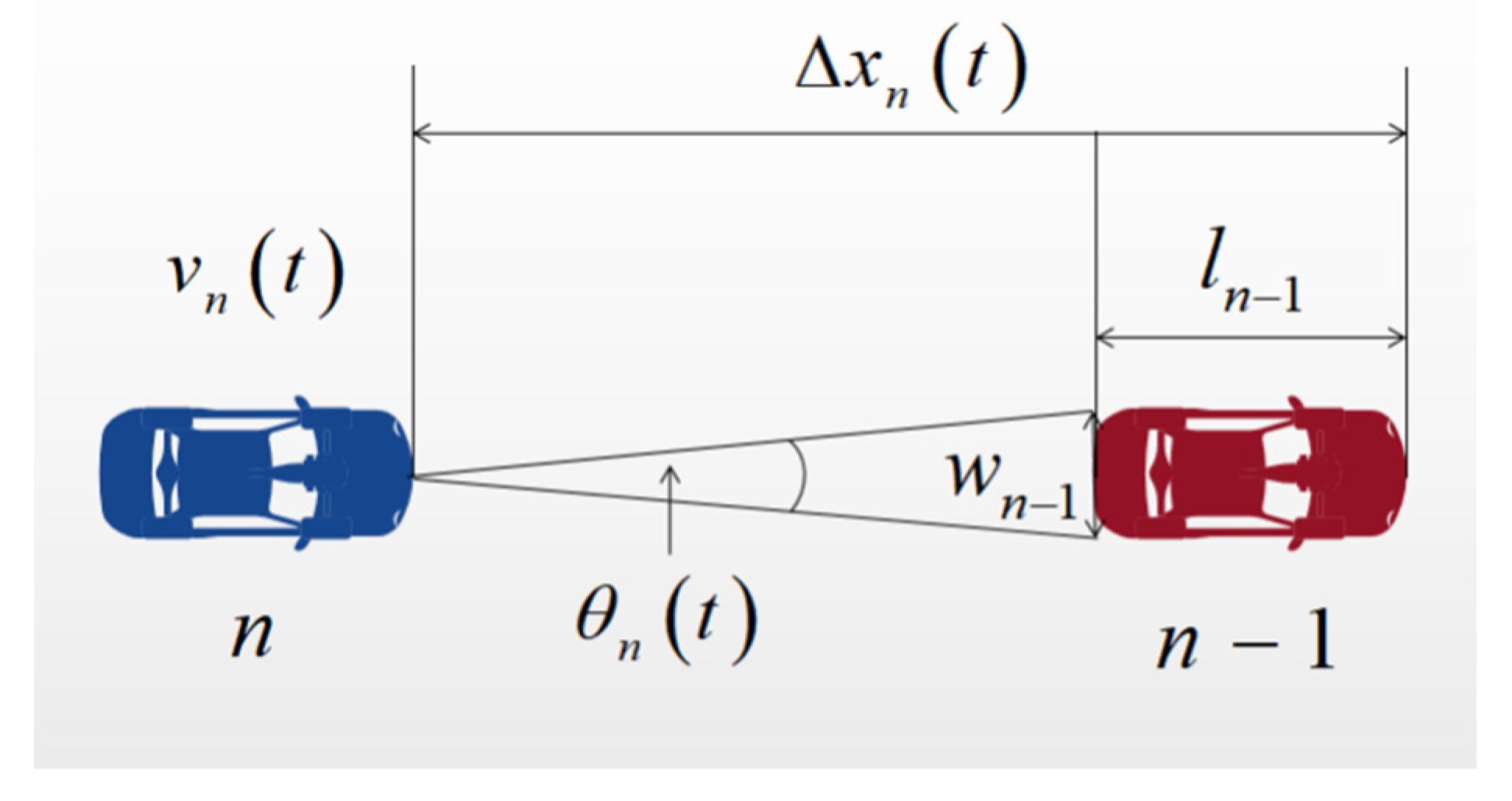
where the speed difference coefficient is expressed as $\lambda$, and the difference in velocity of two successive vehicles is expressed as $\Delta v_n\left(t\right)=v_{n+1}\left(t\right)-v_n\left(t\right)$. All previously proposed models are based on the assumption that the driver’s behavior is perfectly reasonable, and has the ability to accurately sense distance, speed and acceleration. It does not take into account the psychological characteristics of the driver who will change during the follow-up process. Based on the FVD, Jin [41] proposed a visual angle model (VAM), which introduces the follower driver’s perspective into the car-following model by considering the perspective and its rate of change, as shown in Figure 1.

The model formula is as follows:

$$\frac{d{v}_n\left(t\right)}{dt}=\alpha \left[V\left({\theta }_n\left(t\right)\right)-v_n\left(t\right)\right]-\lambda \frac{d}{dt}{\theta }_n\left(t\right)$$

(4)

where the driver’s sensitivity to the difference between the optimal velocity and the current velocity is represented by $\alpha$; the driver’s optimal velocity based on the follower’s perspective is represented by $V\left({\theta }_n(t)\right)$; the angle of view observed by the driver of the $n$-th car at time $t$ is represented by ${\theta }_n\left(t\right)$; the velocity of $n$-th car at time $t$ is represented by $v_n\left(t\right)$; and the sensitivity of the stimulus $d{\theta }_n\left(t\right)/dt$ is represented by $\lambda$.

The driver’s visual angle can be approximated as follows:

$${\theta }_n\left(t\right)=\frac{w_{n-1}}{\Delta x_n\left(t\right)-l_{n-1}}$$

(5)

where $w_{n-1}$ and $l_{n-1}$ are the width and the length of the $\left(n-1\right)$-th car, and $\Delta x_n\left(t\right)$ is the headway between the $n$-th car and $\left(n-1\right)$-th car.

The car-following process is generally limited to a single lane. If the driver sees that the vehicle in front is close to them, the possibility of rear-end collision increases. The stimulus of the preceding vehicle to the driver of the following car prompts the driver of the following car to increase the distance between the two cars. The width and length of the preceding vehicle will also affect the driver’s perspective of judging the traffic situation ahead. If the driver is unable to take precautions against the traffic ahead, out of the psychological stimulus to protect their own safety, the driver of the following vehicle will increase the distance between the two vehicles at this time.

In order to obtain an accurate expression of the driver’s visual angle, assuming that the definition of uniform traffic flow is that all vehicles are moving at the optimal velocity $V\left({\theta }_0\right)$ and the same distance from the preceding vehicle $h$, we use the following formula:

$$x_n^0\left(t\right)=hn+V\left({\theta }_0\right)t$$

(6)

where the optimal velocity is denoted as $V\left({\theta }_0\right)$, the distance headway is expressed as $h$, the position of the $n$-th car is expressed as $x_n^0\left(t\right)$, and the visual angle of the driver of the rear vehicle is expressed as ${\theta }_0\left(t\right)=w_{n-1}/h-l_{n-1}$. Each parameter in the equation is in a stable state. Adding a small disturbance $x_n\left(t\right)=x_n^0\left(t\right)+y_n\left(t\right)$, ${\theta }_n\left(t\right)$ can be rewritten as follows:

$${\theta }_n\left(t\right)=\frac{w_{n-1}}{h+\Delta y_n\left(t\right)-l_{n-1}}=\frac{w_{n-1}\left[\left(h-l_{n-1}\right)-\Delta y_n\left(t\right)\right]}{{\left(h-l_{n-1}\right)}^2-{\left(\Delta y_n\left(t\right)\right)}^2}$$

(7)

Equation (8) can be derived by eliminating the second-order term of $\Delta y_n\left(t\right)$:

$${\theta }_n\left(t\right)=\frac{w_{n-1}}{\left(h-l_{n-1}\right)}-\frac{w_{n-1}\cdot \Delta y_n\left(t\right)}{{\left(h-l_{n-1}\right)}^2}$$

(8)

The follower’s visual angle and its rate of change can be obtained by deriving the derivation of $t$ on both sides of the Equation (8):

$$\frac{d}{dt}{\theta }_n\left(t\right)=-\frac{w_{n-1}}{{\left(h-l_{n-1}\right)}^2}\Delta {y^{\prime }}_n\left(t\right)$$

(9)

Substituting Equation (9) into Equation (4), we can obtain a more intuitive expression of VAM:

$$\frac{d{v}_n\left(t\right)}{dt}=\alpha \left[V\left({\theta }_n(t)\right)-v_n\left(t\right)\right]+\lambda \frac{w_{n-1}}{{\left(h-l_{n-1}\right)}^2}\Delta v_n\left(t\right)$$

(10)

When the vehicle is driving on the road, the visual system is the most important channel for the driver to perceive external information. If the driver observes that the distance between their vehicle and the preceding vehicle gradually becomes smaller, the driver will immediately make adjustments to the current driving behavior.

In addition, the electronic throttle angle is the core variable of the traffic flow stability control system, which is related to the velocity and acceleration of the vehicle. It mainly transmits the operation information of the vehicle in front to the rear, thereby affecting the stability of road traffic. Therefore, considering the above two factors comprehensively, it is closer to the actual traffic situation and provides a reference for road traffic management.

This paper comprehensively considers the two factors of visual angle and electronic throttle effect to make the model closer to the actual traffic situation in the simulation process. Section 2 introduces the influence of the external factor of the angle of view and the internal factor of the electronic throttle on the car-following behavior of the vehicle. Both are taken into account in the car-following model, and its linear stability conditions are provided through calculation and analysis. Section 3 performs a nonlinear analysis near the critical point to derive the TDGL equation. In Section 4, the mKdV equation is provided through calculation and analysis. In Section 5, the factors considered in this paper are numerically simulated by using MATLAB to analyze the impact of information transfer in the actual transportation system. In Section 6, the conclusions are summarized finally.

2. The Extended Model and Linear Stability Analysis

From the driver’s perspective, consider the driver’s attention to the surrounding environment and the psychological pressure caused by the surrounding objects on the driver, and use mathematical models to abstractly express the influence of external objects on the driver’s driving behavior. From the perspective of the automobile structure, the electronic throttle is the core component of the automobile engine operation, and its working performance directly affects the performance of the vehicle.

An electronic throttle system consists of a DC drive (powered by the chopper), a gearbox, a valve plate, a dual return spring, and a position sensor. The driver can control the velocity and acceleration of the vehicle by controlling the angle of the electronic throttle. When the driver steps on the accelerator pedal, it does not directly drive the throttle, but first collects the pedal information and inputs it to the control unit. The control unit drives the throttle valve plate to open and performs precise control of the opening angle according to the input information and the control algorithm pre-stored in it. The proposed model in this paper takes the electronic throttle angle difference of the preceding vehicle into account, which is shown below:

$$\begin{array}{ll}\hfill \frac{d{v}_n\left(t\right)}{dt}=& \alpha \left[V\left({\theta }_n\right)\left(-\frac{w_{n-1}}{{\left(h-l_{n-1}\right)}^2}\Delta x_n\left(t\right)\right)-v_n\left(t\right)\right]+\lambda \frac{w_{n-1}}{{\left(h-l_{n-1}\right)}^2}\Delta v_{n-1}\left(t\right)\hfill \\ & +k\left({\beta }_n\left(t\right)-{\beta }_{n-1}\left(t\right)\right)\hfill \end{array}$$

(11)

The electronic throttle angle difference was quoted by Qin et al. [42]. The mathematical relation between the speed and acceleration and electronic throttle angle is as follows:

$${\beta }_n\left(t\right)=\frac{1}{q}\left[\frac{d{v}_n\left(t\right)}{dt}+p\left(v_n\left(t\right)-v_e\right)\right]+{\beta }_e$$

(12)

where the current balance speed is represented by $v_e$, the current balance electronic throttle angle is represented by ${\beta }_e$, which corresponds to the current balance speed, and $p$ and $q$ both represent constants and are greater than zero.

Calculate the difference between the electronic throttle angle of the $n$-th car and the $\left(n-1\right)$-th car by Equation (12):

$${\beta }_n\left(t\right)-{\beta }_{n-1}\left(t\right)=\frac{1}{q}\left[\frac{d{v}_n\left(t\right)}{dt}-\frac{d{v}_{n-1}\left(t\right)}{dt}+p\left(v_n\left(t\right)-v_{n-1}\left(t\right)\right)\right]$$

(13)

Substituting Equation (13) into Equation (11), the new expression of Equation (11) is calculated as follows:

$$\begin{array}{ll}\hfill \frac{d{v}_n\left(t\right)}{dt}=& \alpha \left[V\left({\theta }_n\right)\left(-\frac{w_{n-1}}{{\left(h-l_{n-1}\right)}^2}\Delta x_n\left(t\right)\right)-v_n\left(t\right)\right]+\lambda \frac{w_{n-1}}{{\left(h-l_{n-1}\right)}^2}\Delta v_{n-1}\left(t\right)\hfill \\ \hfill & +\frac{k}{q}\left[\frac{d{v}_n\left(t\right)}{dt}-\frac{d{v}_{n-1}\left(t\right)}{dt}+p\left(v_n\left(t\right)-v_{n-1}\left(t\right)\right)\right]\hfill \end{array}$$

(14)

where the headway distance between the $\left(n+1\right)$-th car (the preceding car) and the $n$-th car (the rear car) is denoted by $\Delta x_n\left(t\right)=x_{n+1}\left(t\right)-x_n\left(t\right)$, the different sensitivity of each driver is denoted by $\alpha$, and the electronic throttle angle difference coefficient is denoted by $k$.

The optimal velocity function adopts the following formula:

$$V\left({\theta }_n\left(t\right)\right)=V_1+V_2\tanh \left[C_1\left(w_{n-1}/{\theta }_n\left(t\right)\right)-C_2\right]$$

(15)

where the various parameters are calibrated as follows: $V_1=6.75 \mathsf{m}/\mathsf{s}$, $V_2=7.91 \mathsf{m}/\mathsf{s}$, $C_1=0.13 {\mathsf{m}}^{-1}$, $C_2=1.57$. $\Delta x_n=h_c:V^{″}\left(h_c\right)=0$ is the turning point of the increasing function $V(\cdot )$, which has an upper limit.

The TDGL equation can be derived from Equation (14). In order to reduce the difficulty of subsequent nonlinear analysis and improve comprehensibility, Equation (14) is rewritten into a new form:

$$\begin{array}{ll}\hfill \frac{d^2{x}_n\left(t\right)}{d{t}^2}=& \alpha \left[V\left({\theta }_n\right)\left(-\frac{w_{n-1}}{{\left(h-l_{n-1}\right)}^2}\Delta x_n\left(t\right)\right)-\frac{d{x}_n\left(t\right)}{dt}\right]\hfill \\ \hfill & +\lambda \frac{w_{n-1}}{{\left(h-l_{n-1}\right)}^2}\left(\frac{d{x}_n\left(t\right)}{dt}-\frac{d{x}_{n-1}\left(t\right)}{dt}\right)\hfill \\ \hfill & +\frac{k}{q}\left[\frac{d^2{x}_n\left(t\right)}{d{t}^2}-\frac{d^2{x}_{n-1}\left(t\right)}{d{t}^2}+p\left(\frac{d{x}_n\left(t\right)}{dt}-\frac{d{x}_{n-1}\left(t\right)}{dt}\right)\right]\hfill \end{array}$$

(16)

In addition, Equation (16) can be rewritten as a formula with headway as follows:

$$\begin{array}{ll}\hfill \frac{d^2\Delta x_n\left(t\right)}{d{t}^2}=& \alpha [V\left({\theta }_n\right)\left(-\frac{w_{n-1}}{{\left(h-l_{n-1}\right)}^2}\Delta x_{n+1}\left(t\right)\right)-V\left({\theta }_n\right)\left(-\frac{w_{n-1}}{{\left(h-l_{n-1}\right)}^2}\Delta x_n\left(t\right)\right)\hfill \\ \hfill & -\frac{d\Delta x_n\left(t\right)}{dt}]+\lambda \frac{w_{n-1}}{{\left(h-l_{n-1}\right)}^2}\left(\frac{d\Delta x_n\left(t\right)}{dt}-\frac{d\Delta x_{n-1}\left(t\right)}{dt}\right)\hfill \\ \hfill & +\frac{k}{q}\left[\frac{d^2\Delta x_n\left(t\right)}{d{t}^2}-\frac{d^2\Delta x_{n-1}\left(t\right)}{d{t}^2}+p\left(\frac{d\Delta x_n\left(t\right)}{dt}-\frac{d\Delta x_{n-1}\left(t\right)}{dt}\right)\right]\hfill \end{array}$$

(17)

The traffic flow is assumed to reach a steady state. Under this assumption, all vehicles drive forward with a constant headway $h$ and a constant speed $V\left({\theta }_0\right)$. Thus, we will analyze the following equation based on the steady-state solution as follows:

$$x_n^0\left(t\right)=hn+V\left({\theta }_0\right)t,\hspace{1em}h=L/N$$

(18)

where the total number of vehicles is represented by $N$, and the road length is represented by $L$. Assume that $y_n\left(t\right)$ causes a small disturbance to the steady state $x_n\left(t\right)=x_n^0\left(t\right)+y_n\left(t\right)$, and linearizes the equation as follows:

$$\begin{array}{ll}\hfill \frac{d^2{y}_n\left(t\right)}{d{t}^2}& =\alpha \left[V^{\prime }\left({\theta }_0\right)\left(-\frac{w_{n-1}}{{\left(h-l_{n-1}\right)}^2}\Delta y_n\left(t\right)\right)-\frac{d{y}_n\left(t\right)}{dt}\right]\hfill \\ \hfill & +\lambda \frac{w_{n-1}}{{\left(h-l_{n-1}\right)}^2}\left(\frac{d{y}_n\left(t\right)}{dt}-\frac{d{y}_{n-1}\left(t\right)}{dt}\right)\hfill \\ \hfill & +\frac{k}{q}\left[\frac{d^2{y}_n\left(t\right)}{d{t}^2}-\frac{d^2{y}_{n-1}\left(t\right)}{d{t}^2}+p\left(\frac{d{y}_n\left(t\right)}{dt}-\frac{d{y}_{n-1}\left(t\right)}{dt}\right)\right]\hfill \end{array}$$

(19)

where the specific items in the formula are the following: $\Delta y_n\left(t\right)=y_{n+1}\left(t\right)-y_n\left(t\right)$, $V^{\prime }\left({\theta }_0\right)=dV\left(\theta \right)/d\theta {|}_{\theta ={\theta }_0}$. Expanding $y_n\left(t\right)$ with the form of $y_n\left(t\right) = e^{ikn+zt}$, we have the following:

$$\begin{array}{cc}\hfill z^2=& \alpha \left[V^{\prime }\left({\theta }_0\right)\left(-\frac{w_{n-1}}{{\left(h-l_{n-1}\right)}^2}\right)\left(e^{ik}-1\right)-z\right]+\lambda z\frac{w_{n-1}}{{\left(h-l_{n-1}\right)}^2}\left(1-e^{-ik}\right)\hfill \\ \hfill & +\frac{k}{q}\left(z^2\left(1-e^{-ik}\right)+pz\left(1-e^{-ik}\right)\right)\hfill \end{array}$$

(20)

If we set $z=z_1\left(ik\right)+z_2{\left(ik\right)}^2+\cdot \cdot \cdot$ and only retain the first and second order terms of $ik$, then we can obtain the following:

$$z_1=-\frac{w_{n-1}}{{\left(h-l_{n-1}\right)}^2}{V}^{\prime }\left({\theta }_0\right)$$

(21)

$$z_2=-\frac{V^{\prime }\left({\theta }_0\right)w_{n-1}}{\alpha {\left(h-l_{n-1}\right)}^2}\left(\frac{\alpha }{2}+\frac{w_{n-1}\left(\lambda -V^{\prime }\left({\theta }_0\right)\right)}{{\left(h-l_{n-1}\right)}^2}+\frac{\alpha pk}{q}\right)$$

(22)

where $z_2>0$ is the premise of the stability of the initial uniform traffic flow, from which the stability conditions of the new model are calculated as follows:

$$\alpha >\frac{2w_{n-1}\left(\lambda -V^{\prime }\left({\theta }_0\right)\right)}{{\left(h-l_{n-1}\right)}^2}-\frac{2pk}{q}$$

(23)

The neutral stability condition is as follows:

$$\alpha =\frac{2w_{n-1}\left(\lambda -V^{\prime }\left({\theta }_0\right)\right)}{{\left(h-l_{n-1}\right)}^2}-\frac{2pk}{q}$$

(24)

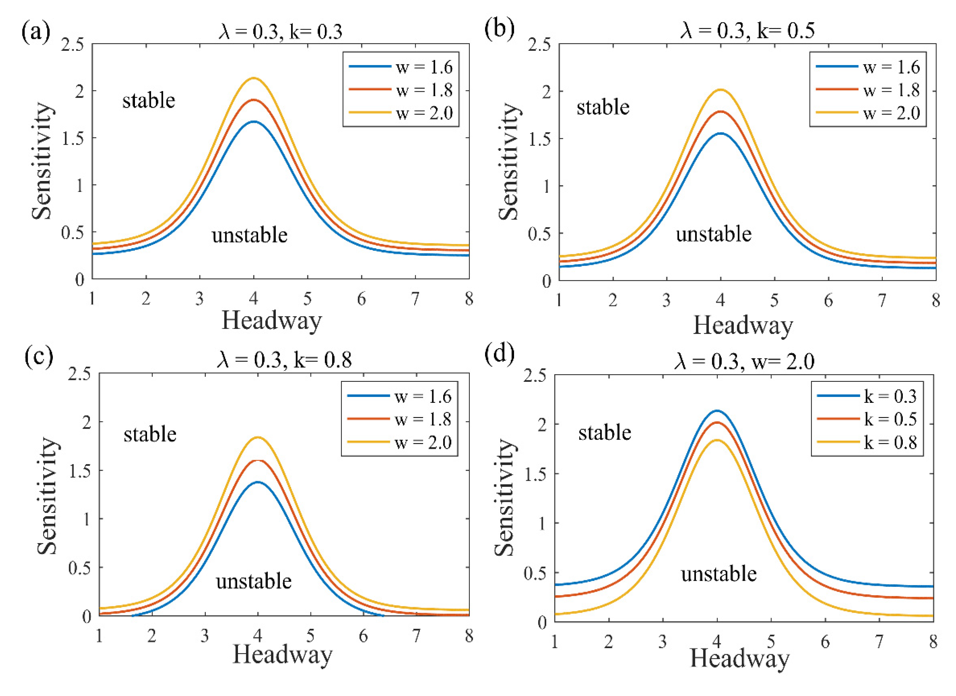
When $\lambda$ and $k$ are fixed, the neutral stability curves with different values of $w=1.8,2.0,2.2$ are as plotted in Figure 2. It considers the potential impact of the vehicle width of the vehicle in front on the transportation system. In the case of the same value, with the width of the vehicle increases, the neutral stability curve moves upward, and the stable area is gradually compressed. It indicates that the increase in vehicle width has caused disturbance to the driver’s visual angle, and visual obstruction increases the psychological pressure of the driver and affects the control of the vehicle. It shows that considering the driver’s angle of view has a negative impact on the steady state operation of the transportation system.

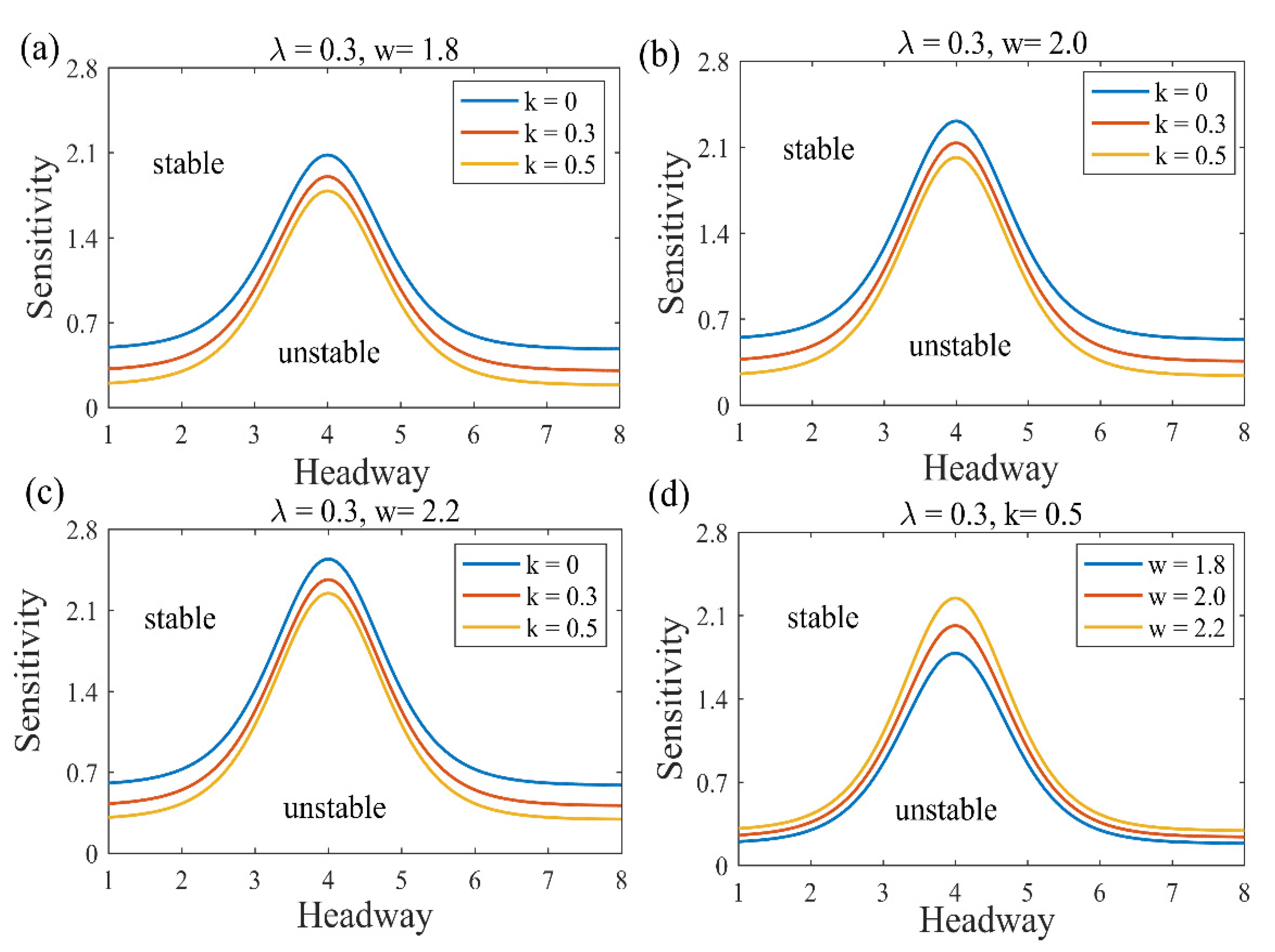
As shown in Figure 3a–c, when $\lambda$ and $w$ are fixed, the stable and unstable regions represented by neutral curves with different $k=0.3, 0.5, 0.8$ values will change. As the value of the coefficient of the electronic throttle angle $k$ increases, the neutral stability curve moves downward, and the stability area gradually expands, indicating that a new factor has a positive impact on the stability of traffic flow. Therefore, considering the electronic throttle angle, the reliability of the system is greatly increased, and the safety of driving is ensured.

Obviously, considering the combined effects of electronic throttle angle and driver’s visual angle, it can effectively alleviate traffic congestion, avoid the occurrence of traffic jams and strengthen the stability of traffic flow, which is in good agreement with the actual road conditions.

3. The TDGL Equation

It is necessary to construct the traffic flow models by which one can derive the TDGL equation since the thermodynamic theory of jamming transition can be formulated by the TDGL equation [43]. In this section, we perform a nonlinear analysis of Equation (17) near the critical point $\left(h_c,{\alpha }_c\right)$ to obtain the TDGL equation describing the traffic behaviors in this extended model. By introducing the slow scale of time variable $t$, space variable $n$ and constant $b$, the following definitions of slow variables $X$ and $T$ are obtained:

$$X=\epsilon \left(n+bt\right), T={\epsilon }^{3}t, 0<\epsilon \ll 1$$

(25)

The headway $\Delta x_n\left(t\right)$ is as follows:

$$\Delta x_n\left(t\right)=h_c+\epsilon R\left(X,T\right)$$

(26)

where $h_c$ stands for safety distance.

By inserting Equations (25) and (26) to Equation (17), as the Taylor expanding to the fifth-order of $\epsilon$, we can obtain the nonlinear partial differential equation as follows:

$$\begin{array}{l}{\epsilon }^2\left(-\frac{w_{n-1}}{{\left(h-l_{n-1}\right)}^2}{V}^{\prime }-b\right){\partial }_{X}R+{\epsilon }^3\left(-\frac{w_{n-1}}{{\left(h-l_{n-1}\right)}^2}\left(\frac{1}{2}{V}^{\prime }+\lambda \tau b\right)+bp\tau \left(\frac{k}{q}-1\right)\right){\partial }_X^{2}R\\ +{\epsilon }^4\left[\left(-\frac{w_{n-1}}{{\left(h-l_{n-1}\right)}^2}\left(\frac{1}{6}{V}^{\prime }+\frac{\lambda \tau b}{2}\right)+\frac{bpk\tau }{2q}\right){\partial }_X^{3}R+\left(-\frac{w_{n-1}}{{\left(h-l_{n-1}\right)}^2}\right)\frac{1}{2}{V}^{‴}{\partial }_X{R}^3-{\partial }_{T}R\right]\\ +{\epsilon }^5\{\left(-\frac{w_{n-1}}{{\left(h-l_{n-1}\right)}^2}\left(\frac{1}{24}{V}^{\prime }-\frac{\lambda \tau b}{6}\right)-\frac{bp\lambda \tau }{3q}\right){\partial }_X^{4}R\\ +\left(-\frac{w_{n-1}}{{\left(h-l_{n-1}\right)}^2}\right)\frac{3}{4}{V}^{‴}{\partial }_X^2{R}^3+\left(\frac{w_{n-1}\lambda \tau }{{\left(h-l_{n-1}\right)}^2}-2\tau b+\frac{k\tau p}{q}\right){\partial }_X{\partial }_{T}R\}=0\end{array}$$

(27)

Traffic behavior is considered to be near the tipping point $\tau =\left(1+{\epsilon }^2\right){\tau }_c$. Eliminating the second-order and third-order terms of $\epsilon$ from Equation (27) by taking $b=\left(-\frac{w_{n-1}}{{\left(h-l_{n-1}\right)}^2}\right)V^{\prime }$, finally the equation is as follows:

$$\begin{array}{cc}\hfill {\epsilon }^4{\partial }_{T}R& = {\epsilon }^4\left(-\frac{w_{n-1}}{{\left(h-l_{n-1}\right)}^2}\left(\frac{1}{6}{V}^{\prime }+\frac{\lambda \tau b}{2}\right)+\frac{bpk\tau }{2q}\right){\partial }_X^{3}R+\left(-\frac{w_{n-1}}{{\left(h-l_{n-1}\right)}^2}\right)\frac{1}{2}{V}^{‴}{\epsilon }^4{\partial }_X{R}^3\hfill \\ \hfill & + {\epsilon }^3\left(-\frac{w_{n-1}}{{\left(h-l_{n-1}\right)}^2}\left(\frac{1}{2}{V}^{\prime }+\lambda \tau b\right)+bp\tau \left(\frac{k}{q}-1\right)\right){\partial }_X^{2}R\hfill \\ & + {\epsilon }^5\left(-\frac{w_{n-1}}{{\left(h-l_{n-1}\right)}^2}\left(\frac{1}{24}{V}^{\prime }-\frac{\lambda \tau b}{6}\right)-\frac{bp\lambda \tau }{3q}\right){\partial }_X^{4}R\hfill \\ \hfill & + {\epsilon }^5\left(-\frac{w_{n-1}}{{\left(h-l_{n-1}\right)}^2}\right)\frac{3}{4}{V}^{‴}{\partial }_X^2{R}^3\hfill \\ \hfill & + {\epsilon }^5\left\{\left(\frac{w_{n-1}\lambda }{{\left(h-l_{n-1}\right)}^2}-2b+\frac{kp}{q}\right)\left(-\frac{w_{n-1}}{{\left(h-l_{n-1}\right)}^2}\left(\frac{1}{6}{V}^{\prime }+\frac{\lambda \tau b}{2}\right)+\frac{bpk\tau }{2q}\right)\right\}{\partial }_X^{4}R\hfill \end{array}$$

(28)

The variables $x={\epsilon }^{-1}X$ and $t={\epsilon }^{-3}T$ are converted by variables $X$ and $T$, and equation $S\left(x,t\right)=\epsilon R\left(X,T\right)$ is established. Equation (28) is finally transformed into the following form:

$$\begin{array}{ll}\hfill {\partial }_{t}S=& \left(-\frac{w_{n-1}}{{\left(h-l_{n-1}\right)}^2}\left(\frac{1}{6}{V}^{\prime }+\frac{\lambda \tau b}{2}\right)+\frac{bpk\tau }{2q}\right){\partial }_x^{3}S+\left(-\frac{w_{n-1}}{{\left(h-l_{n-1}\right)}^2}\right)\frac{1}{2}{V}^{‴}{\partial }_x{S}^3\hfill \\ \hfill & +\left(-\frac{w_{n-1}}{{\left(h-l_{n-1}\right)}^2}\left(\frac{1}{2}{V}^{\prime }+\lambda \tau b\right)+bp\tau \left(\frac{k}{q}-1\right)\right){\partial }_x^{2}S\hfill \\ & +\left(-\frac{w_{n-1}}{{\left(h-l_{n-1}\right)}^2}\left(\frac{1}{24}{V}^{\prime }-\frac{\lambda \tau b}{6}\right)-\frac{bp\lambda \tau }{3q}\right){\partial }_x^{4}S\hfill \\ \hfill & +\left(-\frac{w_{n-1}}{{\left(h-l_{n-1}\right)}^2}\right)\frac{3}{4}{V}^{‴}{\partial }_x^2{S}^3\hfill \\ \hfill & +\left[\left(\frac{w_{n-1}\lambda }{{\left(h-l_{n-1}\right)}^2}-2b+\frac{kp}{q}\right)\left(-\frac{w_{n-1}}{{\left(h-l_{n-1}\right)}^2}\left(\frac{1}{6}{V}^{\prime }+\frac{\lambda \tau b}{2}\right)+\frac{bpk\tau }{2q}\right){\partial }_x^{4}S\right]\hfill \end{array}$$

(29)

By adding term $\left(-\frac{w_{n-1}}{{\left(h-l_{n-1}\right)}^2}\right)\left(-\frac{w_{n-1}}{{\left(h-l_{n-1}\right)}^2}\left(\frac{1}{2}{V}^{\prime }+\lambda \tau b\right)+bp\tau \left(\frac{k}{q}-1\right)\right){\partial }_{x}S$ on two sides of Equation (29) and performing variable conversion $t=t_1$, $x_1=x-\left(-\frac{w_{n-1}}{{\left(h-l_{n-1}\right)}^2}\right)\cdot (\frac{w_{n-1}\left(V^{\prime }\left({\theta }_0\right)-\lambda \right)}{{\left(h-l_{n-1}\right)}^2}\cdot \frac{2q}{2pk+q}){\partial }_{x}S$ for Equation (29), we obtain the following:

$$\begin{array}{ll}\hfill {\partial }_{t_1}S& = \left({\partial }_{x_1}+\left(\frac{1}{2}{V}^{\prime }+\lambda \tau b\right){\partial }_{x_1}^2\right)\hfill \\ \hfill & \times \{\left(-\frac{w_{n-1}}{{\left(h-l_{n-1}\right)}^2}\left(\frac{1}{6}{V}^{\prime }+\frac{\lambda \tau b}{2}\right)+\frac{bpk\tau }{2q}\right){\partial }_{x_1}^{2}S\hfill \\ \hfill & \times (\left(-\frac{w_{n-1}}{{\left(h-l_{n-1}\right)}^2}\left(\frac{1}{2}{V}^{\prime }+\lambda \tau b\right)+bp\tau \left(\frac{k}{q}-1\right)\right)S)+\frac{w_{n-1}}{{\left(h-l_{n-1}\right)}^2}\frac{1}{2}{V}^{‴}{S}^3\}\hfill \end{array}$$

(30)

The thermodynamic potential is defined as follows:

$$\varphi \left(S\right)\equiv -\left(-\frac{w_{n-1}}{{\left(h-l_{n-1}\right)}^2}\right)\left(-\frac{w_{n-1}}{{\left(h-l_{n-1}\right)}^2}\left(\frac{1}{2}{V}^{\prime }+\lambda \tau b\right)+bp\tau \left(\frac{k}{q}-1\right)\right)S^2-\frac{1}{24}{V}^{‴}{S}^4$$

(31)

By rewriting Equation (30) with Equation (31), the following TDGL equation is obtained:

$${\partial }_{t_1}S=-\left({\partial }_{x_1}+\left(\frac{1}{2}{V}^{\prime }+\lambda \tau b\right){\partial }_{x_1}{}^2\right)\frac{\partial \Phi \left(S\right)}{\partial S}$$

(32)

$$\Phi \left(S\right)\equiv {\displaystyle \int d_{x_1}\left[\frac{1}{2}\left(-\frac{w_{n-1}}{{\left(h-l_{n-1}\right)}^2}\left(\frac{1}{6}{V}^{\prime }+\frac{\lambda \tau b}{2}\right)+\frac{bpk\tau }{2q}\right){\left(\partial x_{1}S\right)}^2+\varphi \left(S\right)\right]}$$

(33)

where the function derivative is denoted by $\partial \Phi \left(S\right)/\partial S$. TDGL Equation (32) can obtain a uniform solution, such as Equation (34), and a kink solution, such as Equation (35), when only non-trivial solutions $S\ne 0$ are considered. Both of them are stable solutions:

$$S\left(x_1,t_1\right)=\pm {\left(\frac{\frac{3}{4}\left(-\frac{{\left(h-l_{n-1}\right)}^2}{w_{n-1}}\right)\left(-\frac{w_{n-1}}{{\left(h-l_{n-1}\right)}^2}\left(\frac{1}{2}{V}^{\prime }+\lambda \tau b\right)+bp\tau \left(\frac{k}{q}-1\right)\right)}{V^{‴}}\right)}^{1/2}$$

(34)

$$\begin{array}{ll}\hfill S\left(x_1,t_1\right)& = \pm {\left(\frac{\frac{3}{4}\left(-\frac{{\left(h-l_{n-1}\right)}^2}{w_{n-1}}\right)\left(-\frac{w_{n-1}}{{\left(h-l_{n-1}\right)}^2}\left(\frac{1}{2}{V}^{\prime }+\lambda \tau b\right)+bp\tau \left(\frac{k}{q}-1\right)\right)}{V^{‴}}\right)}^{1/2}\hfill \\ \hfill & \times \tanh \left\{{\left[\left(\frac{w_{n-1}}{{\left(h-l_{n-1}\right)}^2}\left(\frac{1}{24}{V}^{\prime }-\frac{\lambda \tau b}{6}\right)+\frac{bp\lambda \tau }{3q}\right)\left(-\frac{w_{n-1}}{{\left(h-l_{n-1}\right)}^2}\left(\frac{1}{2}{V}^{\prime }+\lambda \tau b\right)\right)\times \left(x_1-x_0\right)\right]}^{1/2}\right\}\hfill \end{array}$$

(35)

where $x_0$ is a constant.

According to Equation (35), we obtain the coexistence curve under the following conditions:

$$\partial \varphi /\partial S=0,\hspace{1em}{\partial }^2\varphi /\partial S^2>0$$

(36)

Equation (31) is substituted into Equation (36) to calculate the coexistence curve, which has the original parameters:

$${\left(\Delta s\right)}_{co}=s_c\pm {\left(\frac{\frac{3}{4}\left(-\frac{{\left(h-l_{n-1}\right)}^2}{w_{n-1}}\right)\left(-\frac{w_{n-1}}{{\left(h-l_{n-1}\right)}^2}\left(\frac{1}{2}{V}^{\prime }+\lambda \tau b\right)+bp\tau \left(\frac{k}{q}-1\right)\right)}{V^{‴}}\right)}^{1/2}$$

(37)

The spinodal line is given by the following condition:

$${\partial }^2\varphi /\partial S^2=0$$

(38)

The spinodal line calculated by substituting Equation (31) into Equation (38) is described by the following:

$${\left(\Delta s\right)}_{sp}=s_c\pm {\left(\frac{\frac{1}{4}\left(-\frac{{\left(h-l_{n-1}\right)}^2}{w_{n-1}}\right)\left(-\frac{w_{n-1}}{{\left(h-l_{n-1}\right)}^2}\left(\frac{1}{2}{V}^{\prime }+\lambda \tau b\right)+bp\tau \left(\frac{k}{q}-1\right)\right)}{V^{‴}}\right)}^{1/2}$$

(39)

The critical point with the original parameters can be obtained by Equation (39) and condition $\partial \varphi /\partial S=0$ as follows:

$${\left(\Delta s\right)}_{co}=h_c, \alpha =\frac{2w_{n-1}\left(\lambda -V^{\prime }\left({\theta }_0\right)\right)}{{\left(h-l_{n-1}\right)}^2}-\frac{2pk}{q}$$

(40)

4. The mKdV Equation

The slow-changing behavior at the long wavelength near the critical point is also worthy of our consideration. In a similar way, we consider the change in traffic behavior near the critical point. The slow scales of the space variable $n$ and the time variable $t$ are extracted with the derivation of the TDGL equation. Eliminating the second and third order terms of $\epsilon$ through taking ${\alpha }_c=\frac{2w_{n-1}\left(\lambda -V^{\prime }\left({\theta }_0\right)\right)}{{\left(h-l_{n-1}\right)}^2}-\frac{2bk}{c}$, ${\alpha }_c=\left(1+{\epsilon }^2\right)\alpha$ into Equation (17), we then obtain the following:

$${\epsilon }^4\left({\partial }_{T}R-g_1{\partial }_X^{3}R-g_2{\partial }_X{R}^3\right)-{\epsilon }^5\left(g_3{\partial }_X^{2}R+g_4{\partial }_X^{4}R+g_5{\partial }_X^2{R}^3\right)=0$$

(41)

where the five coefficients $g_i$ are shown in

Table 1. The coefficients $g_i$ in Equation (41).

$g_1$	$g_2$
$\left(-\frac{w_{n-1}}{{\left(h-l_{n-1}\right)}^2}\left(\frac{1}{6}{V}^{\prime }+\frac{\lambda \tau b}{2}\right)+\frac{bpk\tau }{2q}\right)$	$\left(-\frac{w_{n-1}}{{\left(h-l_{n-1}\right)}^2}\right)\frac{1}{2}{V}^{‴}$
$g_3$	$g_5$
$\left(-\frac{w_{n-1}}{{\left(h-l_{n-1}\right)}^2}\left(\frac{1}{2}{V}^{\prime }+\lambda \tau b\right)+bp\tau \left(\frac{k}{q}-1\right)\right)$	$\left(-\frac{w_{n-1}}{{\left(h-l_{n-1}\right)}^2}\right)\frac{3}{4}{V}^{‴}$
$g_4$
$\left(\frac{w_{n-1}\cdot \lambda }{{\left(h-l_{n-1}\right)}^2}-2b+\frac{kp}{q}\right)\left(-\frac{w_{n-1}}{{\left(h-l_{n-1}\right)}^2}\left(\frac{1}{6}{V}^{\prime }+\frac{\lambda \tau b}{2}\right)+\frac{bpk{\tau }_c}{2q}\right)-\frac{3}{4}{V}^{‴}\left(-\frac{w_{n-1}}{{\left(h-l_{n-1}\right)}^2}\right)\left(-\frac{w_{n-1}}{{\left(h-l_{n-1}\right)}^2}\left(\frac{1}{6}{V}^{\prime }+\frac{\lambda \tau b}{2}\right)+\frac{bpk\tau }{2q}\right)$

below.

In the table $V^{\prime }=dV\left(\Delta x_n\right)/d\Delta x_n|{}_{\Delta x_n=h_c}$ and $V^{‴}=d^{3}V\left(\Delta x_n\right)/d\Delta x_n{}^3|{}_{\Delta x_n=h_c}$. So as to derive the regularized equation, we can perform simple variable conversion:

$$T=\frac{1}{g_1}{T}^{\prime },\hspace{1em}R=\sqrt{\frac{g_1}{g_2}}{R}^{\prime }$$

(42)

So, the standard mKdV equation with $o\left(\epsilon \right)$ correction term is as follows:

$${\partial }_{T^{\prime }}{R}^{\prime }={\partial }_X^3{R}^{\prime }-{\partial }_X{R^{\prime }}^3-\epsilon \left[\frac{g_3}{g_1}{\partial }_X^2{R}^{\prime }+\frac{g_4}{g_1}{\partial }_X^4{R}^{\prime }+\frac{g_5}{g_2}{\partial }_X^2{R^{\prime }}^3\right]$$

(43)

Without considering the $o\left(\epsilon \right)$ term, they only take the kink solution as the mKdV equation of the required solution:

$$R_0^{\prime }\left(X,T^{\prime }\right)=\sqrt{c}\tanh \sqrt{\frac{c}{2}}\left(X-c{T}^{\prime }\right)$$

(44)

Presuming $R^{\prime }\left(X,T^{\prime }\right)=R_0^{\prime }\left(X,T^{\prime }\right)+\epsilon R_1{}^{\prime }\left(X,T^{\prime }\right)$, the $o\left(\epsilon \right)$ correction is considered. So as to define the propagation velocity $c$ for the kink solution, it can be based on the solvability condition. The solvability clause is as follows:

$$\left(R_0^{\prime },M\left[R^{\prime }\right]\right)\equiv {\displaystyle {\int }_{-\infty }^{+\infty }dX{R}_0^{\prime }M\left[R_0^{\prime }\right]}=0$$

(45)

where $M\left[R_0^{\prime }\right]=\frac{g_3}{g_1}{\partial }_X^2{R}^{\prime }+\frac{g_4}{g_1}{\partial }_X^4{R}^{\prime }+\frac{g_5}{g_2}{\partial }_X^2{R^{\prime }}^3$, we obtain the details of the total velocity $c$ as follows:

$$c=\frac{5g_2{g}_3}{2g_2{g}_4-3g_1{g}_5}$$

(46)

Therefore, the mKdV equation is obtained as the general kink–antikink solution of the headway:

$$\Delta x_n\left(t\right)=h_c\pm \sqrt{\frac{g_{1}c}{g_2}\left(\frac{\tau }{{\tau }_c}-1\right)}\times \tanh \sqrt{\frac{c}{2}\left(\frac{\tau }{{\tau }_c}-1\right)}\times \left[n+\left(1-c{g}_1\right)\left(\frac{\tau }{{\tau }_c}-1\right)t\right]$$

(47)

when $V^{‴}<0$, the reciprocal of the driver’s sensitivity coefficient is $\tau$.

The coexisting phase is also represented by a kink solution whose Equation (47) is consistent with that obtained from the TDGL Equation (35). This result indicates that the interference is depicted either by the solution description of the TDGL equation or by the propagation solution of the mKdV equation.

5. Numerical Simulation

Through previous research and the conclusions drawn above, discrete equations can be used in the process of modeling and numerical simulation. We conducted numerical simulations through the computer mathematics software MATLAB. The equation used is as follows:

$$\begin{array}{l}\Delta t^2\left[V\left({\theta }_0\right)\left(\frac{-w_{n-1}}{{\left(h-l_{n-1}\right)}^2}\Delta x_{n+1}(t)\right)-V\left({\theta }_0\right)\left(\frac{-w_{n-1}}{{\left(h-l_{n-1}\right)}^2}\Delta x_n(t)\right)\right]-\Delta t\cdot \frac{-w_{n-1}\lambda \tau }{{\left(h-l_{n-1}\right)}^2}\\ \cdot \left[\Delta x_n\left(t+\Delta t\right)-\Delta x_n\left(t\right)-\left(\Delta x_{n-1}\left(t+\Delta t\right)-\Delta x_{n-1}\left(t\right)\right)\right]+\frac{k\tau }{q}[\Delta x_n\left(t+2\Delta t\right)-2\Delta x_n\left(t+\Delta t\right)\\ +\Delta x_n\left(t\right)-\left(\Delta x_{n-1}\left(t+2\Delta t\right)-2\Delta x_{n-1}\left(t+\Delta t\right)+\Delta x_{n-1}\left(t\right)\right)]\\ +\Delta t\cdot \frac{k\tau p}{q}\left[\Delta x_n\left(t+\Delta t\right)-\Delta x_n\left(t\right)-\left(\Delta x_{n-1}\left(t+\Delta t\right)-\Delta x_{n-1}\left(t\right)\right)\right]=0\end{array}$$

(48)

The initial conditions are the following:

$$\{\begin{array}{l}\Delta x_j\left(0\right)=\Delta x_0=5.0,\hspace{1em}{x}_j\left(1\right)=\Delta x_0=5.0,\hspace{1em}j\ne 50,51.\\ \Delta x_j\left(1\right)=5.0-0.5,\hspace{1em}j=50.\hspace{1em}\\ \Delta x_j\left(1\right)=5.0+0.5,\hspace{1em}j=51.\end{array}$$

(49)

$N=100$ is the total number of vehicles and $\alpha =2$ is the driver’s sensitivity coefficient.

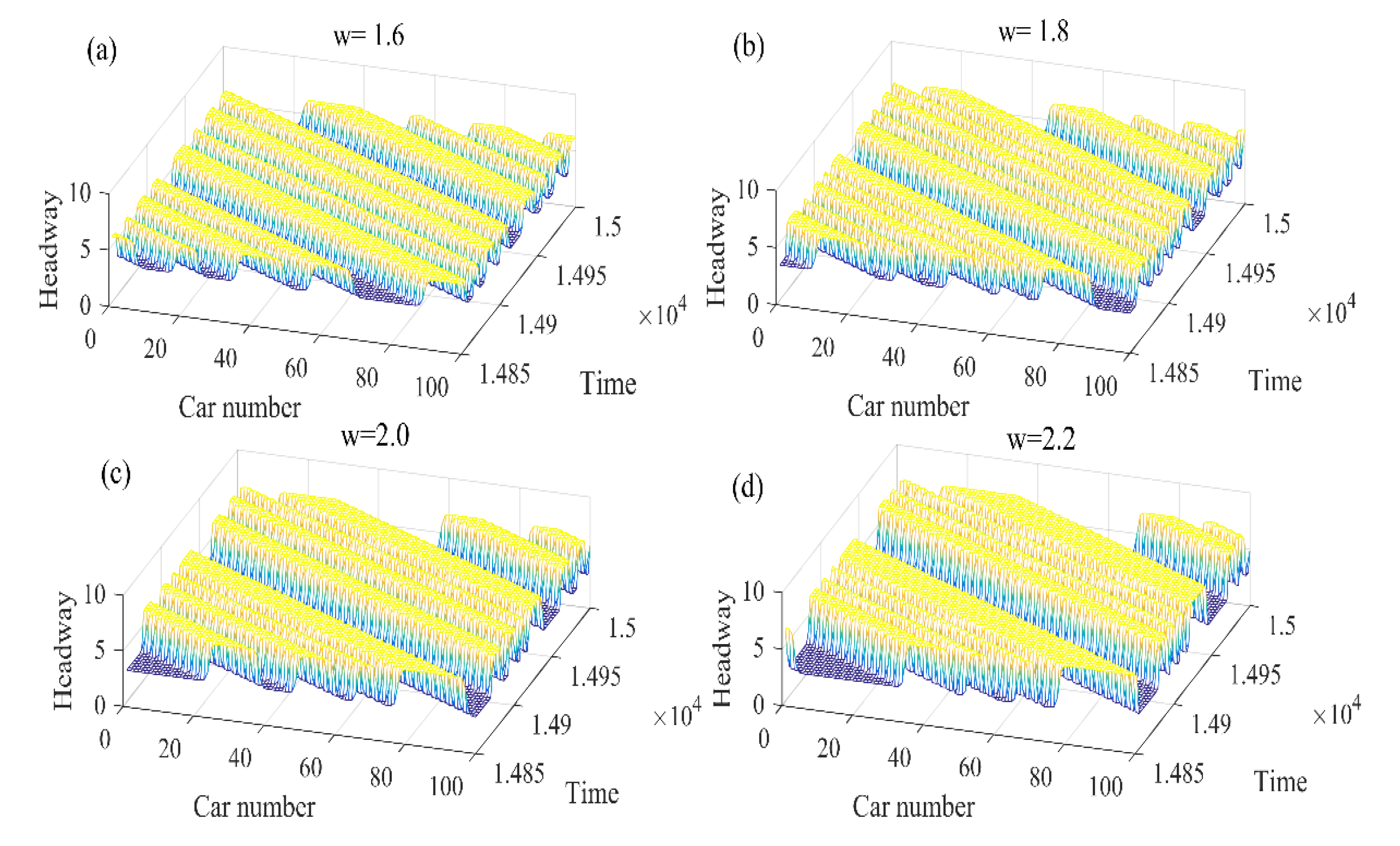
Under the condition of setting different parameters, simulations were performed on the extended model. In Figure 4, under the conditions of different values of $w(w=1.6,1.8,2.0,2.2)$, the evolution results of vehicle flow correspond to the subgraphs in Figure 4a–d, respectively. Especially when $w=1.6$, the traffic flow is in the most stable state that explains the width of the preceding car having a certain influence on the follower’s visual angle. It can be observed and analyzed that with the addition of small disturbances, the initial stable traffic flow transforms into a non-uniform density wave, and the form of this unstable density wave is just the kink–antikink solution of the mKdV equation. It is obvious from the four subgraphs in in Figure 4a–d that the amplitude of the kink–antikink solution gradually decreases with the increase in the parameter $w$. The results show that considering the vehicle width of the preceding vehicle will interfere with the follower’s perspective, which will inevitably affect the stability of the traffic flow. The wider the vehicle width, the more it can interfere with the driver’s perspective and have a negative impact on traffic flow stability.

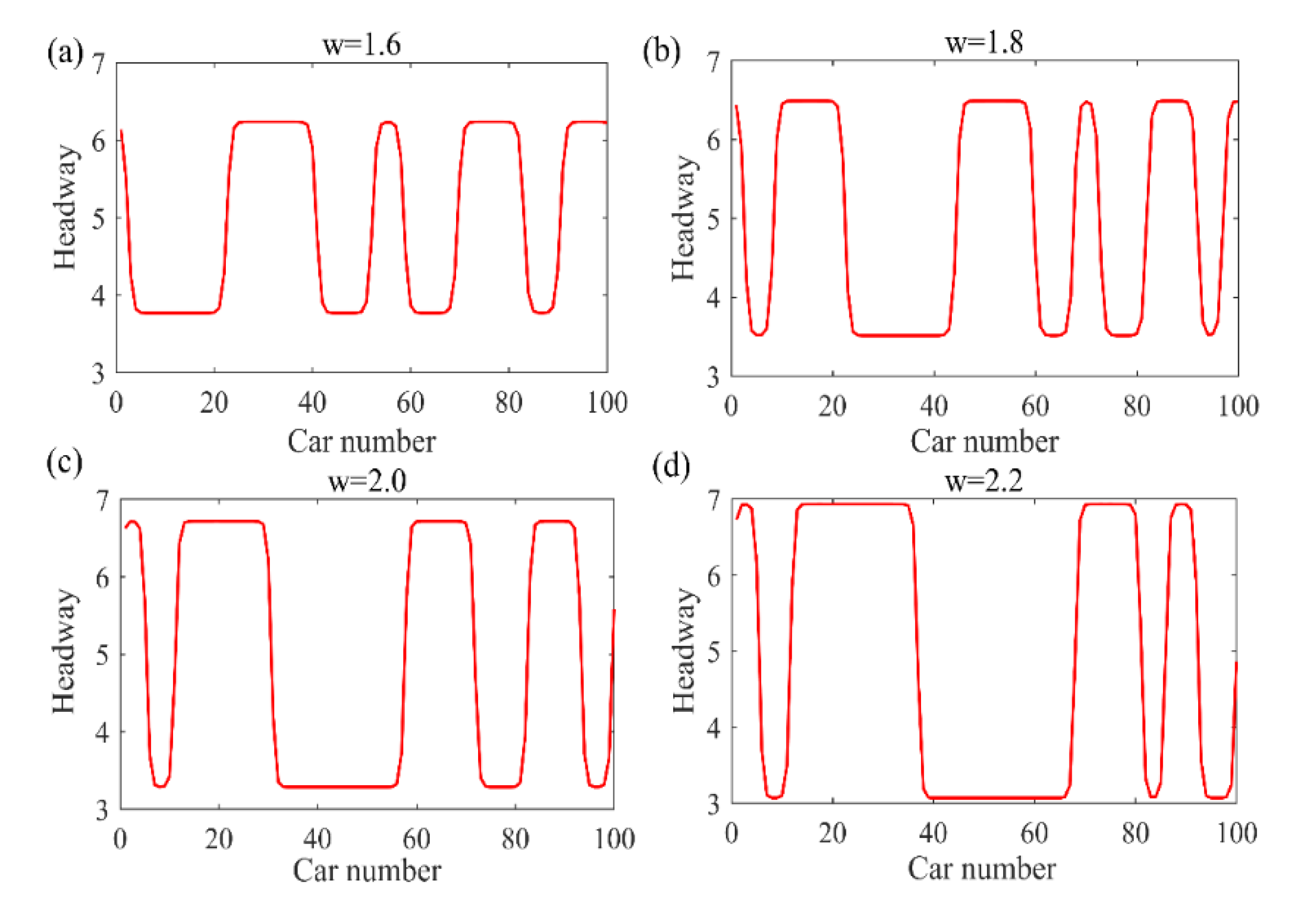
The four sub-pictures in Figure 5a–d correspond to the four sub-pictures in Figure 4a–d, respectively. They are cross-sectional views taken at the same time, representing the headway time-distance distribution and density wave of the preceding vehicle width $w$ at time $t=15,000$. Gradually, as the parameters decrease $w$, the amplitude of the traffic flow becomes smaller. It means that the stability of traffic flow can be positively influenced by considering the information of the width of the preceding vehicle.

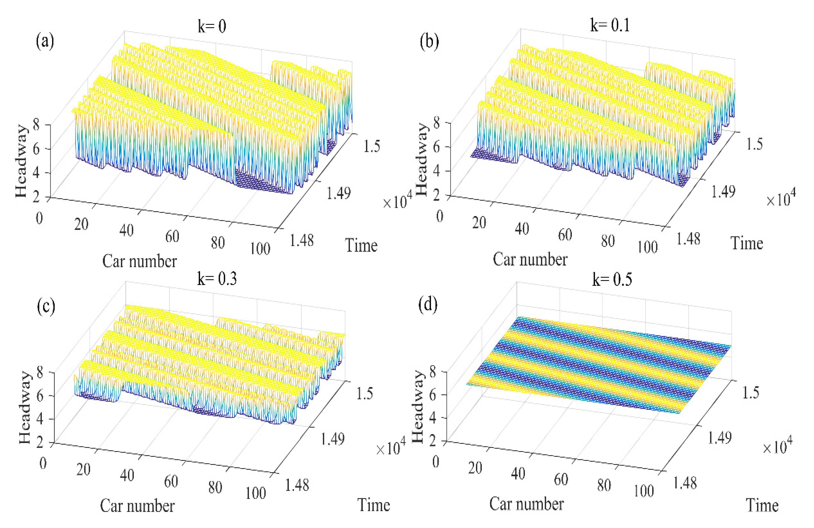
The extended model performed a series of simulations under different electronic throttle angle coefficient coefficients $k(k=0,0.1,0.3,0.5)$, as shown in Figure 6. Electronic throttle can improve the safety, dynamics, stability and economy of car driving, and can effectively alleviate traffic congestion. From the four sub-graphs in Figure 6, the traffic flow is in the most stable state when the electronic throttle angle coefficient is $k=0.5$. It is evident from the subgraphs in Figure 6a–d that the amplitude of the kink-antikink solution decreases with the increase in the angle coefficient of the electronic throttle $k$. It can be observed from the figure that as the fluctuation distance of the traffic flow extends backward, the fluctuation amplitude gradually weakens. The overall trend of traffic flow fluctuations is to reduce to disappear, which shows that considering the handling performance of the vehicle ahead (electronic throttle angle coefficient), the traffic flow can be effectively stabilized. Because the improved model considers the car-following state, it provides a reference for the driver and can adjust the car-following behavior more comprehensively. Therefore, considering the factor of the electronic throttle angle, it is better to provide a reference for the driver, and more fully adjust the current driving state.

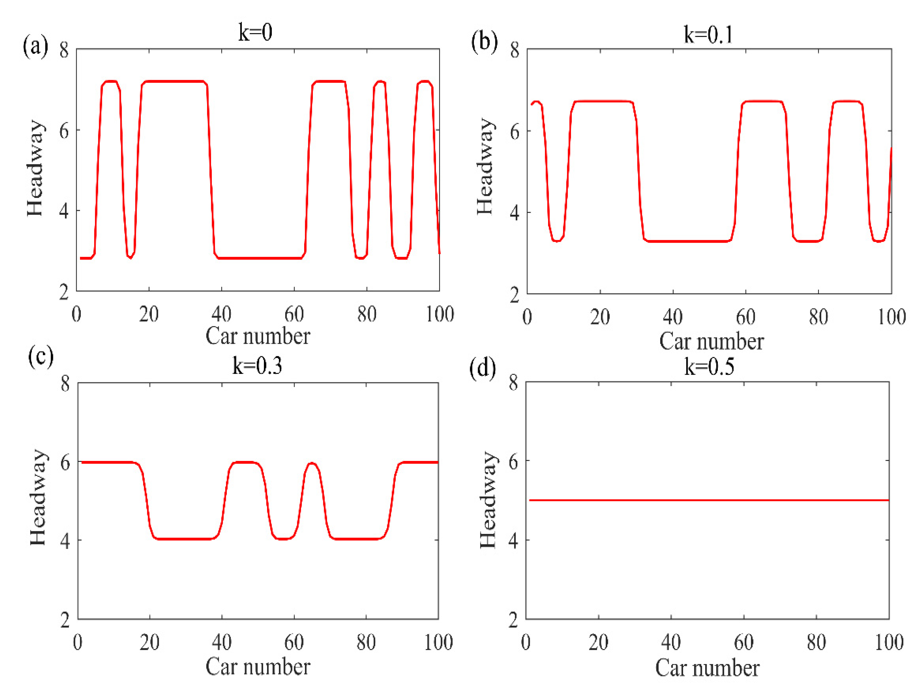
The sub-pictures in Figure 7a–d correspond to the sub-pictures in Figure 6a–d, respectively. They show a cross-sectional view of the fluctuation of traffic flow at a selected moment $t=15,000$, indicating the headway profiles and density wave curve of the electronic throttle angle of the preceding vehicle. From Figure 7a–d, considering the electronic throttle feedback coefficient of the preceding vehicle, the traffic jam can be effectively alleviated, and the traffic interference can be effectively reduced. As the feedback coefficient of the electronic throttle increases, the amplitude of the density wave gradually decreases, and the traffic flow tends to be stable. From the Figure 7, with the adjustment of the parameters, the transportation system can have obvious positive effects.

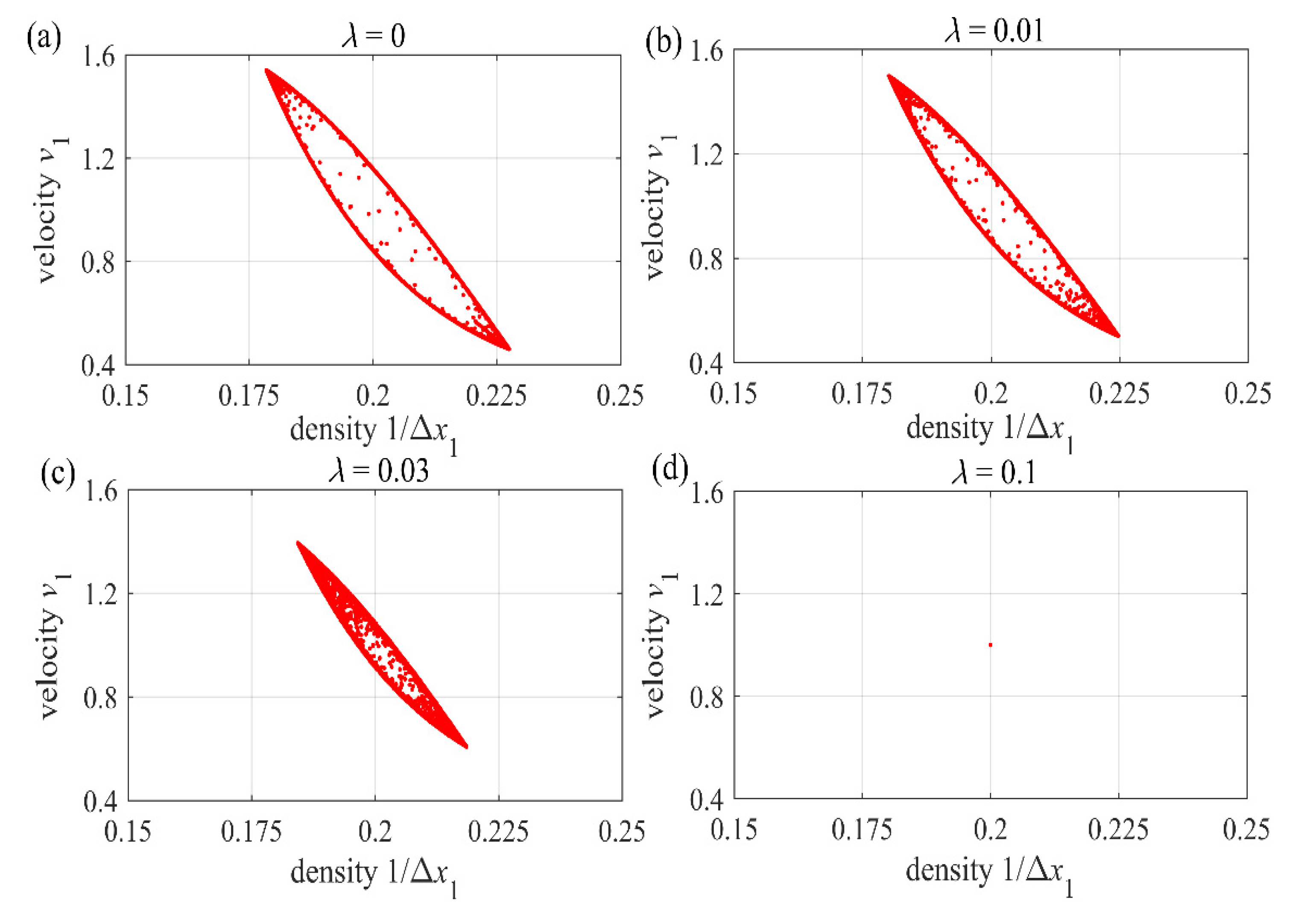
The relationship between the headway distance and the traffic flow, the velocity and the density hysteresis loop relationships are shown in Figure 8, respectively. It shows that as the value increases $\lambda$, the size of the loop decreases. This also indicates that considering the speed difference between the current vehicle and the front vehicle can effectively alleviate urban road traffic congestion, reduce the incidence of accidents, and reduce traffic losses.

6. Conclusions

The model in this paper is based on VAM to describe changes in traffic conditions. From the perspective of the driver, it better combines human factors and achieves a more ideal simulation result. The influence of the electronic throttle angle feedback of the preceding vehicle is taken into consideration. By carrying out linear analysis, neutral stability curves and critical points are obtained. The TDGL equation is obtained by nonlinear analysis, and then the coexistence curve, metastable curve and critical point are described according to the obtained thermodynamic potential. The mKdV equation of the model is obtained by the same method.

Numerical simulation through MATLAB shows that the driver will perceive objects around the vehicle, such as other vehicles, infrastructures and so on, during the driving process. These environmental objects will form a stimulus for the driver (for example, the stimulus of the front vehicle to the driver’s perspective) with varying degrees of intensity. Analyzing and modeling this stimulus will help understand the behavior of the driver during driving. Numerical simulation also shows that the electronic throttle is the core component of automobile engine operation, and its working performance directly affects the performance of the vehicle. Therefore, it is necessary to consider the impact of the electronic throttle angle difference between the preceding vehicle and the current vehicle on the traffic. In the past few decades, the intelligent transportation system (ITS) has achieved rapid development, and the number of cars has also shown a rapid upward trend. Our research helps people better understand the characteristics of traffic flow from the aspects of vehicle external environment and internal structure. This can effectively alleviate traffic congestion, which is of great significance for intelligent highway construction and improving driver’s driving environment. Finally, by comparing the theoretical analysis with numerical simulation, the conclusions are highly consistent.