A Stochastic Harmonic Oscillator Temperature Model for the Valuation of Weather Derivatives

Abstract

Stochastic processes are employed in this paper to capture the evolution of daily mean temperatures, with the goal of pricing temperature-based weather options. A stochastic harmonic oscillator model is proposed for the temperature dynamics and results of numerical simulations and parameter estimation are presented. The temperature model is used to price a one-month call option and a sensitivity analysis is undertaken to examine how call option prices are affected when the model parameters are varied.

1. Introduction

Weather influences our daily lives and affects the volumes of sales and everyday trading in a wide range of businesses. For instance, the powerful typhoons that hit Tokyo and nearby regions in the fall of 2019 caused millions of dollars in damage to infrastructures and extensive damage to agriculture, forestry and fisheries industries [1,2]. Meanwhile, on the other side of the Pacific, the historic cold wave and winter storm of 2021 in Northwest, Central and Eastern America caused an estimated loss of $20.4 billion and represents the most costly U.S. winter storm event on record surpassing (nearly doubling the inflation-adjusted cost) the 93 Superstorm [3]. These two examples are just amongst the many other illustrations of how adverse weather could continuously affect the economy and routinely pose significant financial risks to 70% of all economic sectors worldwide [4].

In the United States, studies show a 1.2% decline in the annual gross domestic product (GDP) for every $1{}^{°}\mathrm{C}$ increase in temperature by the end of this century [5]. While at a global scale, according to the International Monetary Fund, failure to meet a temperature rise to $1.5{}^{°}\mathrm{C}$ may curb the world’s real GDP per capita by roughly 7% by 2100 [6]. Both demonstrate the grave repercussions of Mother Nature that could potentially affect already stressed economies.

To hedge weather-related financial risks, financial instruments called ‘weather derivatives’ were introduced in the financial markets in 1997 in the form of futures, options on futures and swaps [7,8]. The value of such a derivative is based on some underlying weather-dependent variable such as wind speed, amount of snowfall or rainfall and temperature levels. Financial products have been developed for industries facing business uncertainty as a result of weather fluctuations, allowing companies to trade and hedge those risks caused by weather volatility.

In these exotic weather derivative contracts, the payoffs depend on the chosen weather index, reflecting the weather conditions against which protection is needed. The largest portion of traded weather derivatives are written on temperature-based indices. Clearly, the temperature does not have a price in itself and therefore is not a tradeable asset. As a consequence, following the standard derivative pricing theoretical framework, the valuation of these derivatives relies heavily on the appropriate modelling of the index. This context motivates the purpose of this work, that is, to propose an easy-to-calibrate stochastic temperature model that does not require specific meteorological background and inputs. Hence, the model can be straightforwardly implemented by practitioners in the financial industry.

Several approaches have been developed for weather derivative pricing problems, such as time series [9,10], stochastic discount factor models [11,12] and lattices [13].

We follow a stochastic modelling approach in this paper. Previous results in this direction are due to Benth and Saltyte-Benth [14], Dornier and Querel [15], Brody et al. [16] and Alaton et al. [17]. All of these papers put forward a mean reverting Ornstein–Uhlenbeck process to describe the temperature fluctuations, some of which are driven by fractional Brownian motion or generalised Lévy processes instead of standard Brownian motion.

It can be argued whether in the aforementioned results it is sufficient to describe the temperature dynamics by a single stochastic process. Since observed temperature data indicate a seasonality trend, we will deviate from the previous approaches and consider as our starting point the classical harmonic oscillator model [18], which is described by a second-order ordinary differential equation (ODE). We will convert this model to a system of two coupled stochastic differential equations (SDEs) with two driving Wiener processes. The system will turn out to be still analytically tractable and we fit our stochastic harmonic oscillator model to actual temperature data. Using a risk-neutral framework, we will price weather derivatives, more specifically, a call option on an underlying variable which is a temperature-based index.

The outline of this paper is as follows: in Section 2, we derive a stochastic temperature model based on the classical harmonic oscillator and compare it to a popular stochastic temperature model. Section 3 presents numerical simulations of the proposed model, as well as results of parameter estimation using theoretical and real temperature data. In Section 4, we use the temperature model to price a one-month call option and perform a sensitivity analysis to examine how call option prices are affected when the model parameters are varied. We provide brief concluding remarks in Section 5.

2. Derivation of a Stochastic Harmonic Oscillator Temperature Model

Let $T\left(t\right)\in \mathbb{R}$ denote the daily average temperature at time $t\ge 0$. We begin by considering a general (deterministic) sinusoidal function of time, namely

$$T\left(t\right)=Asin(Bt+C)+D,$$

where $A,B,C,D\in \mathbb{R}$ and $A,B\ne 0$. It can be shown that $T\left(t\right)$ satisfies the ODE

$$\frac{{\mathrm{d}}^{2}T}{\mathrm{d}{t}^2}+k^{2}T=a,$$

(1)

where $k=B$ and $a=B^{2}D$. Without loss of generality, we may take $k>0$ and $a\in \mathbb{R}$. Let $x_1\left(t\right)=T\left(t\right)$ and $x_2\left(t\right)=T^{\prime }\left(t\right)$. Then, (1) can be written as a system of two first-order ODEs

$$\frac{\mathrm{d}{x}_1}{\mathrm{d}t}=x_2,\frac{\mathrm{d}{x}_2}{\mathrm{d}t}=-k^2{x}_1+a,$$

which in differential form is equivalent to

$$\begin{array}{cc}\hfill \mathrm{d}{x}_1\left(t\right)& =x_2\left(t\right)\mathrm{d}t,\hfill \\ \hfill \mathrm{d}{x}_2\left(t\right)& =[-k^2{x}_1\left(t\right)+a]\mathrm{d}t.\hfill \end{array}$$

(2)

We introduce randomness in (2) as follows. Consider the following system for the stochastic processes $X_1=\{X_1\left(t\right):t\ge 0\}$ and $X_2=\{X_2\left(t\right):t\ge 0\}$:

$$\begin{array}{cc}\hfill \mathrm{d}{X}_1\left(t\right)& =X_2\left(t\right)\mathrm{d}t+{\sigma }_1\mathrm{d}{W}_1\left(t\right),\hfill \\ \hfill \mathrm{d}{X}_2\left(t\right)& =[-k^2{X}_1\left(t\right)+a]\mathrm{d}t+{\sigma }_2\mathrm{d}{W}_2\left(t\right),\hfill \end{array}$$

(3)

where ${\sigma }_1,{\sigma }_2\ge 0$ are parameters that control the size of the fluctuations and $W_1=\{W_1\left(t\right):t\ge 0\}$ and $W_2=\{W_2\left(t\right):t\ge 0\}$ are (possibly correlated) standard Wiener processes. Equation (3) can be expressed in matrix form as

$$\mathrm{d}\mathbf{X}\left(t\right)=\left[\mathbf{A}\mathbf{X}\right(t)+\mathbf{B}]\mathrm{d}t+\mathbf{C}\mathrm{d}\mathbf{W}\left(t\right),$$

where

$$\mathbf{A}=\left(\begin{array}{cc}0& 1\\ -k^2& 0\end{array}\right),\mathbf{B}=\left(\begin{array}{c}0\\ a\end{array}\right),\mathbf{C}=\left(\begin{array}{cc}{\sigma }_1& 0\\ 0& {\sigma }_2\end{array}\right)$$

and

$$\mathbf{X}\left(t\right)=\left(\begin{array}{c}{X}_1\left(t\right)\\ X_2\left(t\right)\end{array}\right),\mathbf{W}\left(t\right)=\left(\begin{array}{c}{W}_1\left(t\right)\\ W_2\left(t\right)\end{array}\right).$$

From Evans [19], we can write the solution of (3) as

$$\mathbf{X}\left(t\right)={\mathrm{e}}^{t\mathbf{A}}{\mathbf{X}}_0+{\int }_0^t{\mathrm{e}}^{(t-u)\mathbf{A}}\mathbf{B}\mathrm{d}u+{\int }_0^t{\mathrm{e}}^{(t-u)\mathbf{A}}\mathbf{C}\mathrm{d}\mathbf{W}\left(u\right),$$

(4)

where ${\mathrm{e}}^{t\mathbf{A}}$ is the matrix exponential of $\mathbf{A}$ and ${\mathbf{X}}_0=\mathbf{X}\left(0\right)$. The eigenvalues of $\mathbf{A}$ are easily seen to be $\pm \mathrm{i}k$. Recalling the explicit formula for the matrix exponential [20], we obtain

$${\mathrm{e}}^{t\mathbf{A}}=\left(\begin{array}{cc}cos\left(kt\right)& \frac{1}{k}sin\left(kt\right)\\ -ksin\left(kt\right)& cos\left(kt\right)\end{array}\right)$$

and therefore

$${\mathrm{e}}^{t\mathbf{A}}\mathbf{B}=\left(\begin{array}{c}\frac{a}{k}sin\left(kt\right)\\ acos\left(kt\right)\end{array}\right),{\mathrm{e}}^{t\mathbf{A}}\mathbf{C}=\left(\begin{array}{cc}{\sigma }_{1}cos\left(kt\right)& \frac{{\sigma }_2}{k}sin\left(kt\right)\\ -{\sigma }_{1}ksin\left(kt\right)& {\sigma }_{2}cos\left(kt\right)\end{array}\right).$$

Since in the deterministic model (2) we have $x_1\left(t\right)=T\left(t\right)$, for the stochastic model (3), we associate $X_1\left(t\right)=T\left(t\right)$. Therefore, taking the first component in (4) and setting ${\theta }_1=X_1\left(0\right)$ and ${\theta }_2=X_2\left(0\right)$, we get

$$\begin{array}{cc}\hfill X_1\left(t\right)& ={\theta }_{1}cos\left(kt\right)+\frac{{\theta }_2}{k}sin\left(kt\right)+{\int }_0^t\frac{a}{k}sin\left(k(t-u)\right)\mathrm{d}u\hfill \\ \hfill & +{\int }_0^t{\sigma }_{1}cos\left(k(t-u)\right)\mathrm{d}{W}_1\left(u\right)+{\int }_0^t\frac{{\sigma }_2}{k}sin\left(k(t-u)\right)\mathrm{d}{W}_2\left(u\right).\hfill \end{array}$$

Thus, our stochastic harmonic oscillator temperature model is

$$\begin{array}{cc}\hfill T\left(t\right)& =\frac{a}{k^2}+\left({\theta }_1-\frac{a}{k^2}\right)cos\left(kt\right)+\frac{{\theta }_2}{k}sin\left(kt\right)\hfill \\ \hfill & +{\sigma }_1{\int }_0^{t}cos\left(k(t-u)\right)\mathrm{d}{W}_1\left(u\right)+\frac{{\sigma }_2}{k}{\int }_0^{t}sin\left(k(t-u)\right)\mathrm{d}{W}_2\left(u\right).\hfill \end{array}$$

(5)

By renaming the parameters in (5), we can write

$$\begin{array}{cc}\hfill T\left(t\right)& =c_0+c_{1}cos\left(kt\right)+c_{2}sin\left(kt\right)\hfill \\ \hfill & +c_3{\int }_0^{t}cos\left(k(t-u)\right)\mathrm{d}{W}_1\left(u\right)+c_4{\int }_0^{t}sin\left(k(t-u)\right)\mathrm{d}{W}_2\left(u\right).\hfill \end{array}$$

(6)

We wish to estimate the parameters k and $c_j$ for $j=0,1,2,3,4$ by calibrating (6) to temperature data.

Remark 1.

Dornier and Querel [15] and Alaton et al. [17] assumed that the daily average temperature is modelled by

$$T\left(t\right)=S\left(t\right)+X\left(t\right).$$

(7)

The term $S\left(t\right)$ is the deterministic seasonal component of the form

$$S\left(t\right)=at+b+\sum _{j=1}^3\left[c_{j}sin\left(2^{j-1}\frac{2\pi t}{365}\right)+d_{j}cos\left(2^{j-1}\frac{2\pi t}{365}\right)\right],$$

where a, b, $c_j$ and $d_j$ for $j=1,2,3$ are constants to be determined. The stochastic deseasonalised component is described by the stochastic process $X=\left\{X\right(t):t\ge 0\}$, where

$$\mathrm{d}X\left(t\right)=\lambda [\mu -X(t\left)\right]\mathrm{d}t+\sigma \mathrm{d}W\left(t\right)$$

and $W=\left\{W\right(t):t\ge 0\}$ is a standard Wiener process. The parameters λ, μ and σ denote the mean reversion rate, long term average and volatility, respectively, of the process X. It is well known that X is an Ornstein–Uhlenbeck process and

$$X\left(t\right)=\mu +[X\left(0\right)-\mu ]{\mathrm{e}}^{-\lambda t}+\sigma {\mathrm{e}}^{-\lambda t}{\int }_0^t{\mathrm{e}}^{\lambda u}\mathrm{d}W\left(u\right).$$

Thus, the expected value of $T\left(t\right)$ in (7) is

$$E\left(T\left(t\right)\right)=S\left(t\right)+\mu +[X\left(0\right)-\mu ]{\mathrm{e}}^{-\lambda t}.$$

Note that this is not periodic in t. Comparing (7) with (5), we see that in (5) there are two driving Wiener processes $W_1$ and $W_2$. Moreover, the expected value of $T\left(t\right)$ in (5) is

$$E\left(T\left(t\right)\right)=\frac{a}{k^2}+\left({\theta }_1-\frac{a}{k^2}\right)cos\left(kt\right)+\frac{{\theta }_2}{k}sin\left(kt\right),$$

(8)

which is a periodic function of t and shows that the deterministic component of the temperature would also satisfy a harmonic oscillator ODE.

The model we propose here is different from other two-factor models in the literature as (5) is obtained from the system (3), which in turn is a stochastic analogue of the harmonic oscillator model (1). In contrast, Hell et al. [21] established a general theoretical framework for the pricing of temperature derivatives by consistent factor models. Groll et al. [22] provided an empirical back-up for the theoretical framework introduced by Hell et al. [21] and put their pricing approach into practice.

3. Numerical Simulations of a Stochastic Harmonic Oscillator Temperature Model

In this section, we show the results of various numerical simulations of the models (5) and (3). All simulations are done in Scilab (see https://www.scilab.org, accessed on 12 October 2021), a free and open-source, cross-platform programming language.

Fix $t_{\max }>0$ and define $\mathrm{\Delta }t=\frac{t_{\max }}{n-1}$, where $n>1$ is chosen to be a ‘large’ integer. If $u_j=(j-1)\mathrm{\Delta }t$ for $j=1,2,\dots ,n$, then we see that $u_1=0$ and $u_n=t_{\max }$. Thus, $\{u_1,u_2,\dots ,u_n\}$ is an equidistant partition of the interval $[0,t_{\max }]$.

3.1. Simulation of a Stochastic Integral as a Stochastic Process

If f is a deterministic function of t and u, where $t,u\in [0,t_{\max }]$, and $W=\{W\left(t\right):0\le t\le t_{\max }\}$ is a Wiener process, then we use the Riemann–Stieltjes approximation

$$\begin{array}{cc}\hfill & {\int }_0^{t_{\max }}f(t,u)\mathrm{d}W\left(u\right)\simeq \sum _{j=1}^{n-1}f(t,u_j)[W\left(u_{j+1}\right)-W\left(u_j\right)]\hfill \\ \hfill & =\sum _{j=2}^{n-1}f(t,u_j)[W\left(u_{j+1}\right)-W\left(u_j\right)]+f(t,0)[W\left(u_2\right)-W\left(u_1\right)]\hfill \\ \hfill & =\sum _{j=2}^{n-1}f(t,u_j)[W\left(u_{j+1}\right)-W\left(u_j\right)]+f(t,0)W\left(u_2\right).\hfill \end{array}$$

Note that $W\left(u_1\right)=W\left(0\right)=0$ since W is a Wiener process. Moreover, $W\left(u_{j+1}\right)-W\left(u_j\right)\sim N(0,\mathrm{\Delta }t)$ for all $j=1,2,\dots ,n-1$.

As

$${\int }_0^{t}f(t,u)\mathrm{d}W\left(u\right)={\int }_0^{t_{\max }}f(t,u){\mathbf{1}}_{[0,t)}\left(u\right)\mathrm{d}W\left(u\right),$$

where ${\mathbf{1}}_{[0,t)}$ is the indicator function of the set $[0,t)$, we deduce that

$$\begin{array}{cc}\hfill {\int }_0^{t}f(t,u)\mathrm{d}W\left(u\right)& \simeq \sum _{j=2}^{n-1}f(t,u_j){\mathbf{1}}_{[0,t)}\left(u_j\right)[W\left(u_{j+1}\right)-W\left(u_j\right)]\hfill \\ \hfill & +f(t,0){\mathbf{1}}_{[0,t)}\left(0\right)W\left(u_2\right)\hfill \\ \hfill & =\sum _{j=2}^{n-1}f(t,(j-1)\mathrm{\Delta }t){\mathbf{1}}_{[0,t)}\left((j-1)\mathrm{\Delta }t\right)[W\left(u_{j+1}\right)-W\left(u_j\right)]\hfill \\ \hfill & +f(t,0)W\left(u_2\right).\hfill \end{array}$$

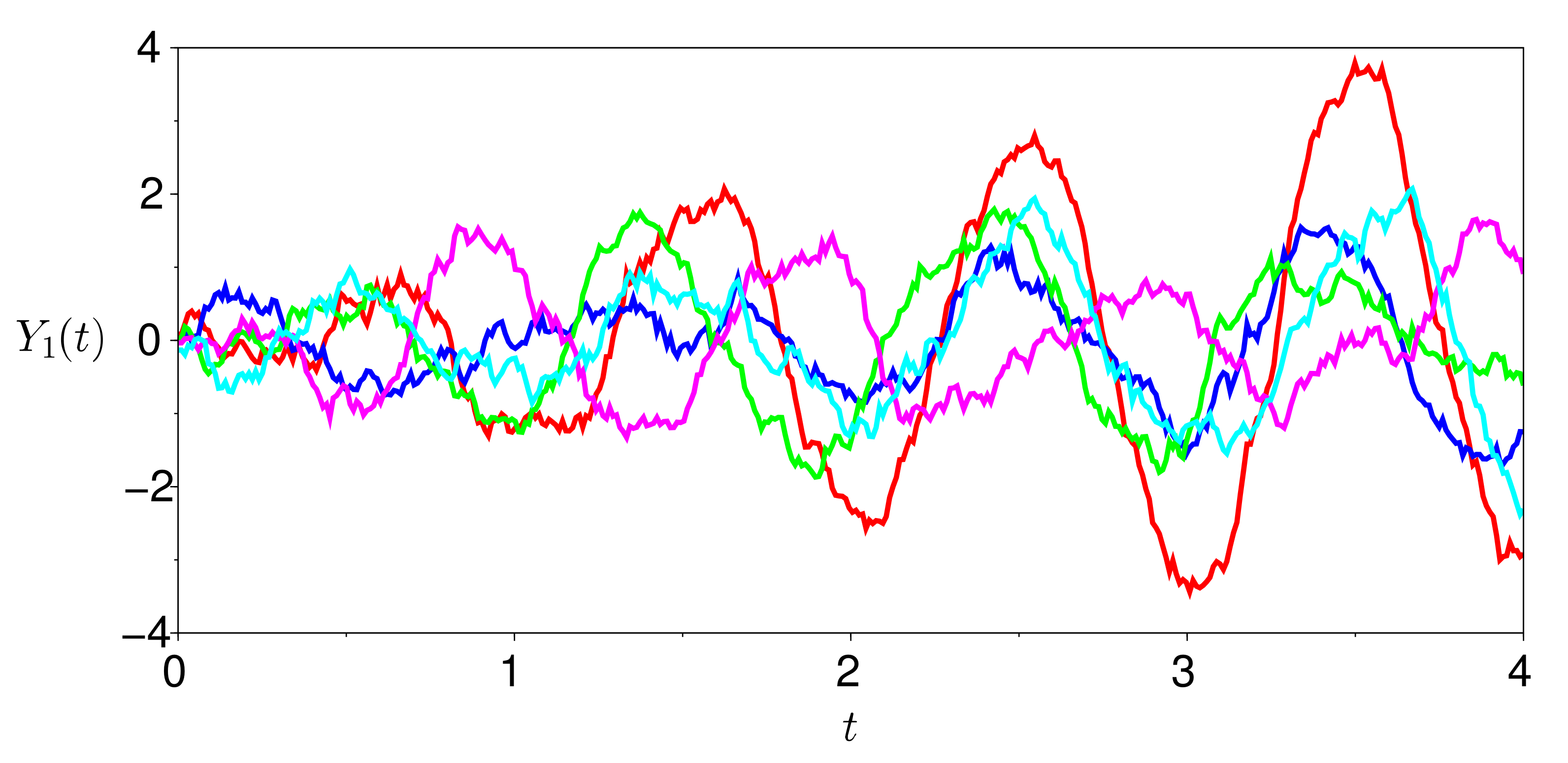
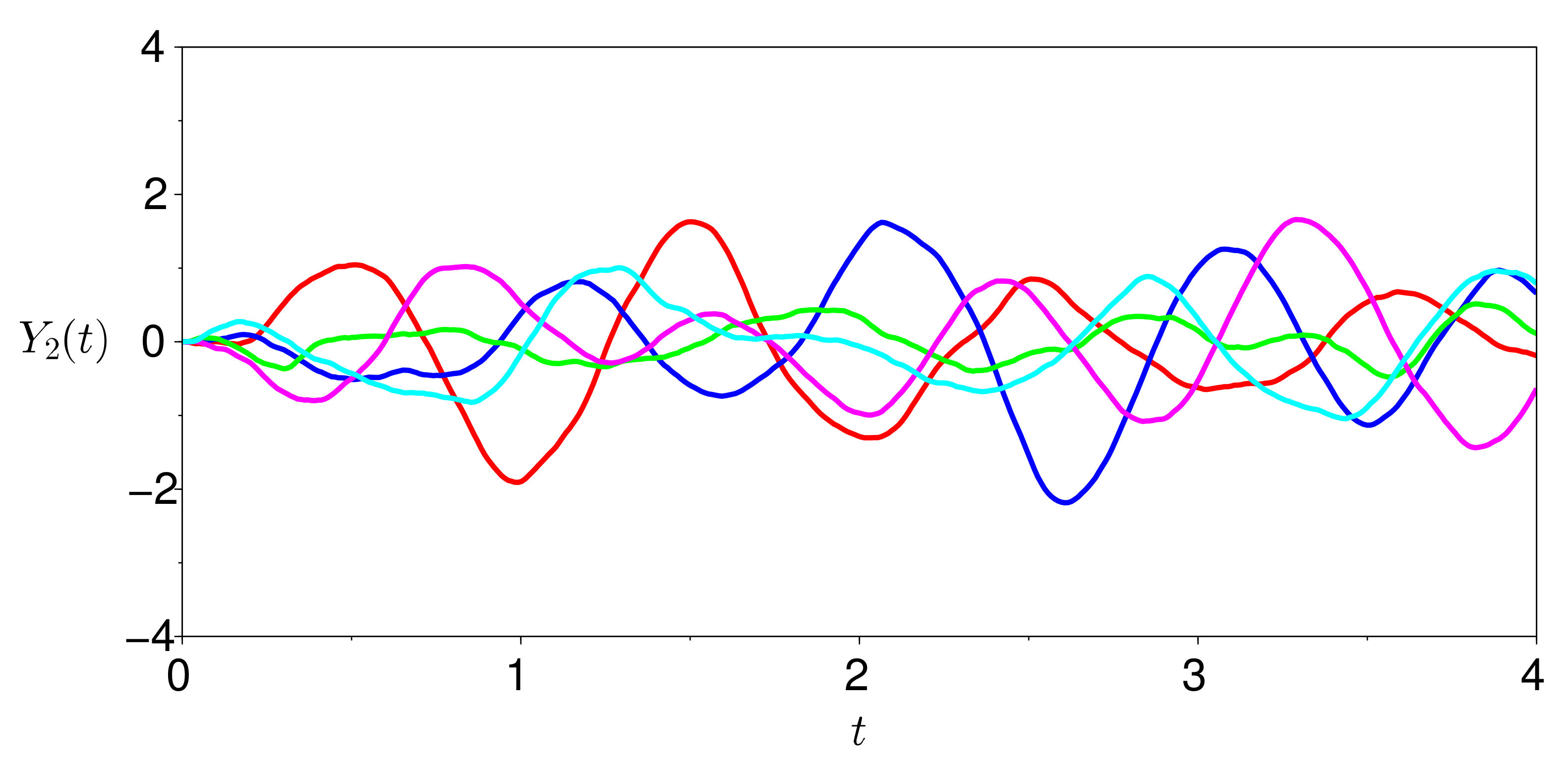
For example, suppose that we take $n=400$ and $t_{\max }=4$. Then, sample paths of $Y_1=\{Y_1\left(t\right):0\le t\le 4\}$ and $Y_2=\{Y_2\left(t\right):0\le t\le 4\}$, where

$$Y_1\left(t\right)={\int }_0^{t}cos\left(2\pi (t-u)\right)\mathrm{d}W\left(u\right)$$

(9)

and

$$Y_2\left(t\right)={\int }_0^{t}sin\left(2\pi (t-u)\right)\mathrm{d}W\left(u\right),$$

(10)

are shown in Figure 1 and Figure 2, respectively. We observe that the sample paths of $Y_1$ are more ‘jagged’ than those of $Y_2$.

3.2. Simulation of a Stochastic Harmonic Oscillator Temperature Model

To simulate the stochastic process $T=\left\{T\right(t):0\le t\le 4\}$, where $T\left(t\right)$ is given in (5), take $n=1000$ and $t_{\max }=4$. Then, choose

$$a=2,k=6,{\theta }_1=0,{\theta }_2=-1,{\sigma }_1=2.5,{\sigma }_2=1.$$

(11)

We generate two correlated Wiener processes $W_1=\{W_1\left(t\right):0\le t\le 4\}$ and $W_2=\{W_2\left(t\right):0\le t\le 4\}$ such that

$$W_2\left(t\right)=\rho W_1\left(t\right)+\sqrt{1-{\rho }^2}W\left(t\right)$$

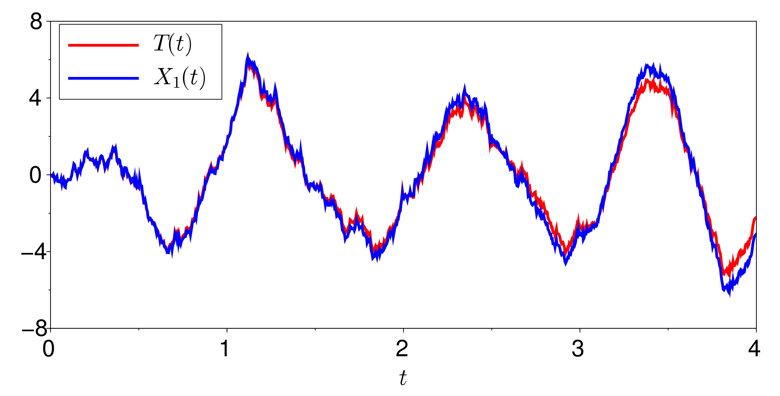
and $\rho \in [-1,1]$ is the correlation coefficient. Choose $\rho =0.5$ for definiteness. A sample path for the process T is represented by the red graph in Figure 3.

Next, we solve the system (3) using the Euler–Maruyama algorithm. We remark that the Milstein and Euler–Maruyama schemes are equivalent for this model. Define the functions

$$\begin{array}{cc}\hfill & a_1(t,x_1,x_2)=x_2,b_1(t,x_1,x_2)={\sigma }_1,\hfill \\ \hfill & a_2(t,x_1,x_2)=-k^2{x}_1+a,b_2(t,x_1,x_2)={\sigma }_2.\hfill \end{array}$$

Setting $t_j=(j-1)\mathrm{\Delta }t$ for $j=1,2,\dots ,n$, we see that $X_1\left(t_1\right)=X_1\left(0\right)={\theta }_1$ and $X_2\left(t_1\right)=X_2\left(0\right)={\theta }_2$. For $j=1,2,\dots ,n-1$, we compute recursively

$$\begin{array}{cc}\hfill X_1\left(t_{j+1}\right)& =X_1\left(t_j\right)+a_1(t_j,X_1\left(t_j\right),X_2\left(t_j\right))\mathrm{\Delta }t\hfill \\ \hfill & +b_1(t_j,X_1\left(t_j\right),X_2\left(t_j\right))[W_1\left(t_{j+1}\right)-W_1\left(t_j\right)],\hfill \\ \hfill X_2\left(t_{j+1}\right)& =X_2\left(t_j\right)+a_2(t_j,X_1\left(t_j\right),X_2\left(t_j\right))\mathrm{\Delta }t\hfill \\ \hfill & +b_2(t_j,X_1\left(t_j\right),X_2\left(t_j\right))[W_2\left(t_{j+1}\right)-W_2\left(t_j\right)].\hfill \end{array}$$

Plotting the first component of the approximate solution yields the blue graph in Figure 3. As expected, the plots are relatively close to each other since we identify $X_1$ with T. The $L^2$-norm of the difference between the sample paths of $X_1$ and T is $16.77$. Choosing a larger n may decrease the error at the cost of a slower computational speed.

3.3. Parameter Estimation for a Stochastic Harmonic Oscillator Temperature Model Using Theoretical Data

The next step is to fit (5) using theoretical data. As before, let $n=1000$ and $t_{\max }=4$, while assuming the parameters in (11). We use (5) to generate a set of theoretical data $\{T_j:j=1,2,\dots ,1000\}$, where $T_j=T\left(t_j\right)=T\left((j-1)\mathrm{\Delta }t\right)$ for $j=1,2,\dots ,1000$. The profile of the theoretical temperature curve is given by the red curve in Figure 4, which is actually hidden behind the blue curve. Then, with the exception of $k=6$ in (11), we ‘pretend’ that all of the parameters a, ${\theta }_1$, ${\theta }_2$, ${\sigma }_1$ and ${\sigma }_2$ are unknown and we attempt to fit (5) to the theoretically generated data.

Since the data set $\{(t_j,T_j):j=1,2,\dots ,n\}$ is known and the Wiener processes $W_1$ and $W_2$ can be generated, and we assume for now that k is given, then the stochastic integrals

$${\int }_0^{t_j}cos\left(k(t_j-u)\right)\mathrm{d}{W}_1\left(u\right),{\int }_0^{t_j}sin\left(k(t_j-u)\right)\mathrm{d}{W}_2\left(u\right)$$

appearing in (6) are also known for each $j=1,2,\dots ,n$ because they can be computed as in Section 3.1. It is therefore convenient to use (6) since this equation is linear in the parameters $c_0$, $c_1$, $c_2$, $c_3$ and $c_4$ if we further replace $T\left(t\right)$ by $T_j$, $cos\left(kt\right)$ by $cos\left(k{t}_j\right)$ and $sin\left(kt\right)$ by $sin\left(k{t}_j\right)$. Then, a standard multi-dimensional linear regression can be implemented to estimate these parameters. That is, if $Y={\left(\begin{array}{ccc}{T}_1& \cdots & T_n\end{array}\right)}^{*}$ (where ${(·)}^{*}$ denotes the matrix transpose) and

$$X=\left(\begin{array}{ccccc}1& cos\left(k{t}_1\right)& sin\left(k{t}_1\right)& {\int }_0^{t_1}cos\left(k(t_1-u)\right)\mathrm{d}{W}_1\left(u\right)& {\int }_0^{t_1}sin\left(k(t_1-u)\right)\mathrm{d}{W}_2\left(u\right)\\ 1& cos\left(k{t}_2\right)& sin\left(k{t}_2\right)& {\int }_0^{t_2}cos\left(k(t_2-u)\right)\mathrm{d}{W}_1\left(u\right)& {\int }_0^{t_2}sin\left(k(t_2-u)\right)\mathrm{d}{W}_2\left(u\right)\\ ⋮& ⋮& ⋮& ⋮& ⋮\\ 1& cos\left(k{t}_n\right)& sin\left(k{t}_n\right)& {\int }_0^{t_n}cos\left(k(t_n-u)\right)\mathrm{d}{W}_1\left(u\right)& {\int }_0^{t_n}sin\left(k(t_n-u)\right)\mathrm{d}{W}_2\left(u\right)\end{array}\right),$$

then

$${\left(\begin{array}{ccccc}{\widehat{c}}_0& {\widehat{c}}_1& {\widehat{c}}_2& {\widehat{c}}_3& {\widehat{c}}_4\end{array}\right)}^{*}={\left(X^{*}X\right)}^{-1}{X}^{*}Y.$$

The result is

$${\widehat{c}}_0=0.06,{\widehat{c}}_1=-0.06,{\widehat{c}}_2=-0.17,{\widehat{c}}_3=2.50,{\widehat{c}}_4=0.17.$$

In terms of the original parameters, we obtain

$$\widehat{a}=2.00,{\widehat{\theta }}_1=0.00,{\widehat{\theta }}_2=-1.00,{\widehat{\sigma }}_1=2.50,{\widehat{\sigma }}_2=1.00.$$

Using these estimated parameters in (5) generates a set $\{{\widehat{T}}_j:j=1,2,\dots ,1000\}$ and is represented by the blue curve in Figure 4. As the original parameters in (11) have been recovered, this explains why the blue curve lies on top of the red curve. The $L^2$-norm of the difference between $\{T_j:j=1,2,\dots ,1000\}$ and $\{{\widehat{T}}_j:j=1,2,\dots ,1000\}$ is $0.00$. For comparison, the green curve in Figure 4 is obtained from (5) but without the stochastic integral terms, i.e., (8).

Remark 2.

Earlier, we assumed that k was known. Now suppose that k is unknown. Assuming for the moment that the stochastic integral terms in (5) are negligible, the ‘period’ P can be estimated through

$$P=\frac{2\pi }{k}\mathrm{or}k=\frac{2\pi }{P}.$$

In Figure 3, we see that there is a ‘crest’ that starts at around $t=2.60$ and ends at around $t=3.60$. Taking $P\simeq 3.60-2.60=1.00$, then $k\simeq 6.28$. This could be taken as the k fixed in the above linear regression. However, a more reasonable approach is to assume that k lies within some range, say $5\le k\le 7$, and test different values of k ranging from $k=5$ to $k=7$. For each such fixed k, we apply linear regression as above and compute the $L^2$-error between $\{T_j:j=1,2,\dots ,1000\}$ and $\{{\widehat{T}}_j:j=1,2,\dots ,1000\}$. When the $L^2$-error is less than some predetermined tolerance, the corresponding k is chosen and the rest of the parameters a, ${\theta }_1$, ${\theta }_2$, ${\sigma }_1$ and ${\sigma }_2$ are estimated.

3.4. Parameter Estimation for a Stochastic Harmonic Oscillator Temperature Model Using Real Data

In this section, we use a data set of daily mean temperatures observed at the Toronto Pearson International Airport located in Mississauga, Ontario, Canada and compiled by the National Climatic Data Center (NCDC) (see http://www.ncdc.noaa.gov/cdo-web/datasets, accessed on 12 October2021) of the United States Department of Commerce. The period considered is from January 2005 to December 2008, for a total of 1461 data points. Each daily mean temperature is obtained by taking the average of the lowest and highest temperature readings for that day and converting from ${}^{°}\mathrm{F}$ to ${}^{°}\mathrm{C}$.

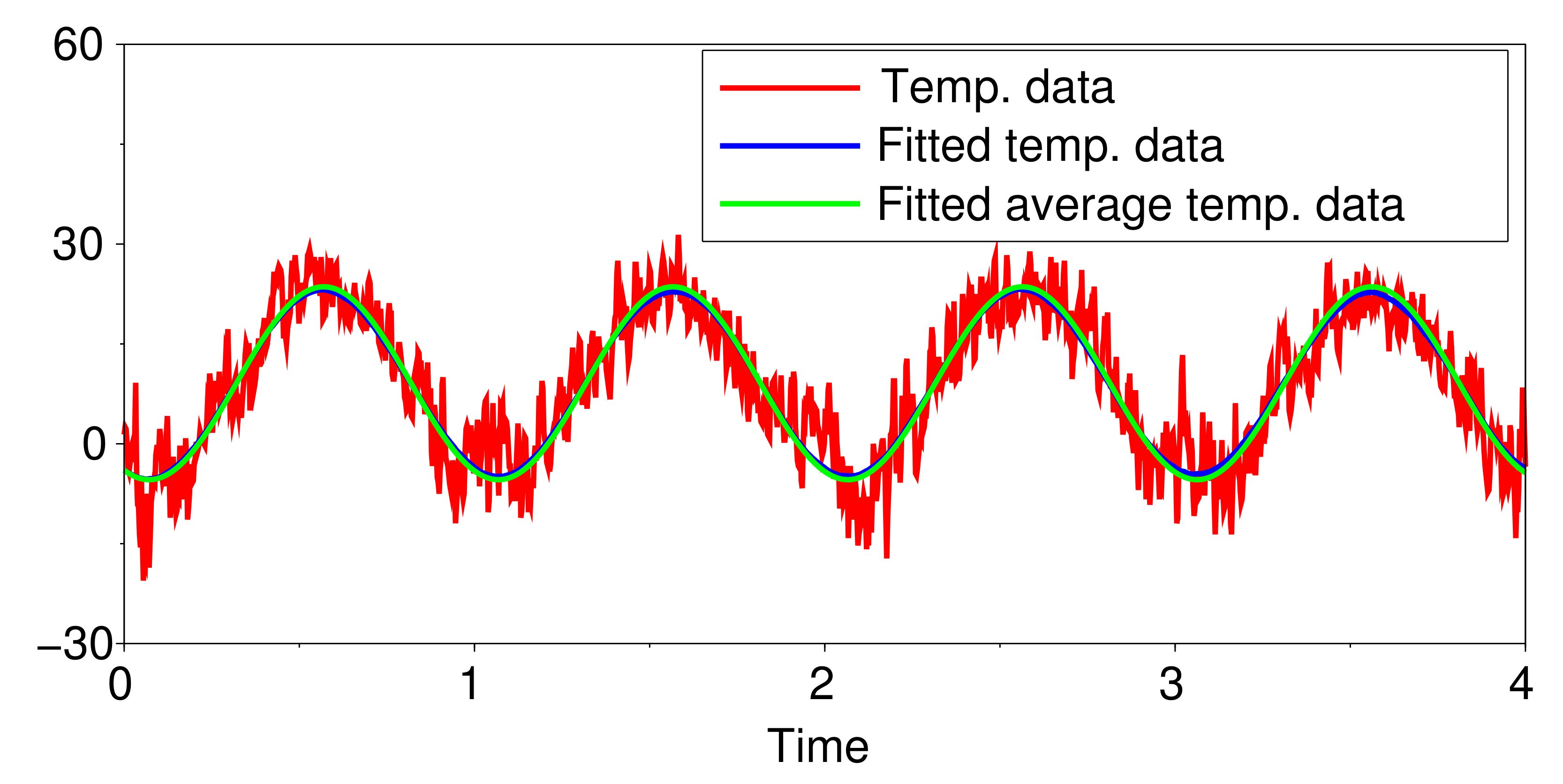
Denote by n the number of days of observed temperature data. Let

$$t_j=(j-1)\mathrm{\Delta }t,j=1,2,\dots ,n,\mathrm{\Delta }t=\frac{1}{365}\frac{n}{n-1}.$$

Note that $t_j$ will be expressed in years and $t_n=(n-1)\mathrm{\Delta }t=\frac{n}{365}$. In this case, $n=1461$ and $t_{\max }=t_n=t_{1461}=4$. Fix $k=6.3$ (an explanation for this choice will be provided in Remark 3 below). Following the procedure described in Section 3.3, the estimated parameters are

$$\widehat{a}=358.55,{\widehat{\theta }}_1=-4.14,{\widehat{\theta }}_2=-33.69,{\widehat{\sigma }}_1=0.45,{\widehat{\sigma }}_2=1.64.$$

(12)

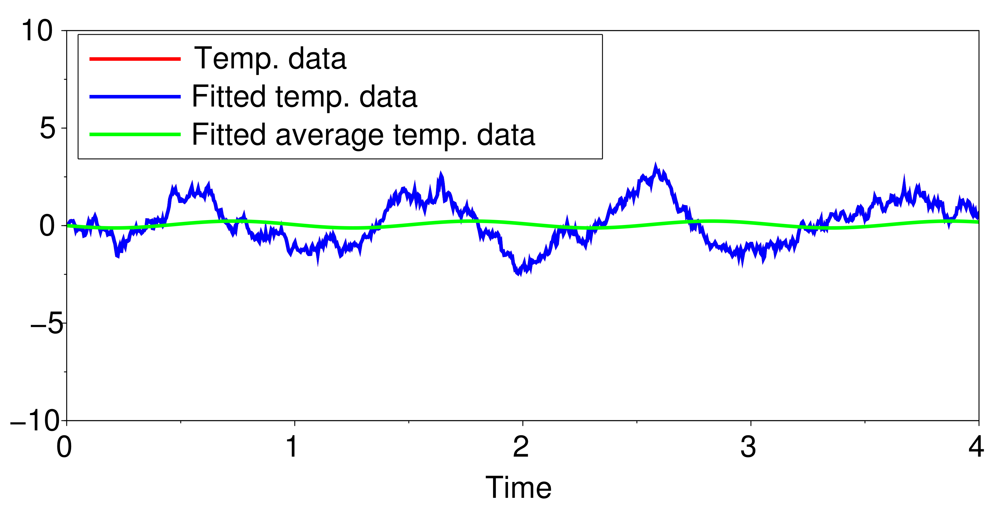
In Figure 5, the red graph is the observed temperature data $\{T_j:j=1,2,\dots ,1461\}$ while the blue curve (behind the green curve) is the fitted temperature data $\{{\widehat{T}}_j:j=1,2,\dots ,1461\}$, i.e., (5) with the parameters replaced by the estimated parameter values in (12). The green curve is (5) but without the stochastic integral terms, which is equivalent to $\{E\left({\widehat{T}}_j\right):j=1,2,\dots ,1461\}$ from (8).

Unlike in Figure 4, the fitted temperature data in Figure 5 is not too ‘jagged’ but is actually close to $E\left(T\right(t\left)\right)$. This can be seen from the fact that $0<{\widehat{\sigma }}_1<{\widehat{\sigma }}_2$. Hence, in (5), the contribution from the stochastic integral with the cos integrand is not as pronounced as that from the stochastic integral with the sin integrand. As pointed out previously for Figure 1 and Figure 2, the stochastic integral with the sin integrand tends to produce less ‘jagged’ sample paths.

Remark 3.

The $L^2$-norm of the difference between $\{T_j:j=1,2,\dots ,1461\}$ and $\{{\widehat{T}}_j:j=1,2,\dots ,1461\}$ is $167.20$. Following the explanation given in Remark 2, the value $k=6.3$ was chosen because it produced the smallest $L^2$-error amongst all the values of k taken from $k=5$ to $k=7$ in increments of $\mathrm{\Delta }k=0.1$.

4. Pricing of Weather Derivatives

4.1. Basics of a Weather Derivative Contract

A standard weather derivative contract typically has the following elements [8]:

• contract period (traded contracts are seasonal and monthly);
• weather-based variable (contracts are based on temperature, snowfall, rainfall, etc.);
• measurement station (e.g., La Guardia Airport, New York City);
• index (e.g., HDD or CDD);
• payoff function (makes it possible to convert the index to cash flow);
• tick (multiplier for each weather index point).

The underlying indices of these contracts, from which these financial instruments derive their value, represent the biggest difference with respect to other financial derivatives. There are two major types of indices used for temperature. The first is the cumulative average temperature (CAT), which is the sum of the daily average temperature values throughout the contract period. The other major type is an index based on degree days. Heating degree days (HDD) is a measurement of the amount the daily temperature falls below a set baseline B (typically, $B=18{}^{°}\mathrm{C}=65{}^{°}\mathrm{F}$), accumulated over the contract period. Cooling degree days (CDD) is similar to HDD but measures the amount the daily temperature exceeds B.

Suppose that n is the number of days over which the HDD/CDD index is considered. Let $T_j$ denote the average of the maximum and minimum temperatures observed on day j, where $j=1,2,\dots ,n$. Then,

$$\begin{array}{cc}\hfill \mathrm{HDD}& =\mathrm{HDD}\left(n\right)=\sum _{j=1}^{n}max(B-T_j,0),\hfill \\ \hfill \mathrm{CDD}& =\mathrm{CDD}\left(n\right)=\sum _{j=1}^{n}max(T_j-B,0).\hfill \end{array}$$

(13)

These indices were originally created by the energy industry as a proxy for the domestic demand for heating and cooling. The motivation for the above formulas is that, when the temperature is above (respectively, below) the baseline, people would consume energy on cooling (respectively, heating) appliances but not on heating (respectively, cooling) appliances.

At the Chicago Mercantile Exchange (CME), HDD contracts are traded from January to April and from October to December, while CDD contracts are traded from April to October. Months in which both indices are traded are known as shoulder months.

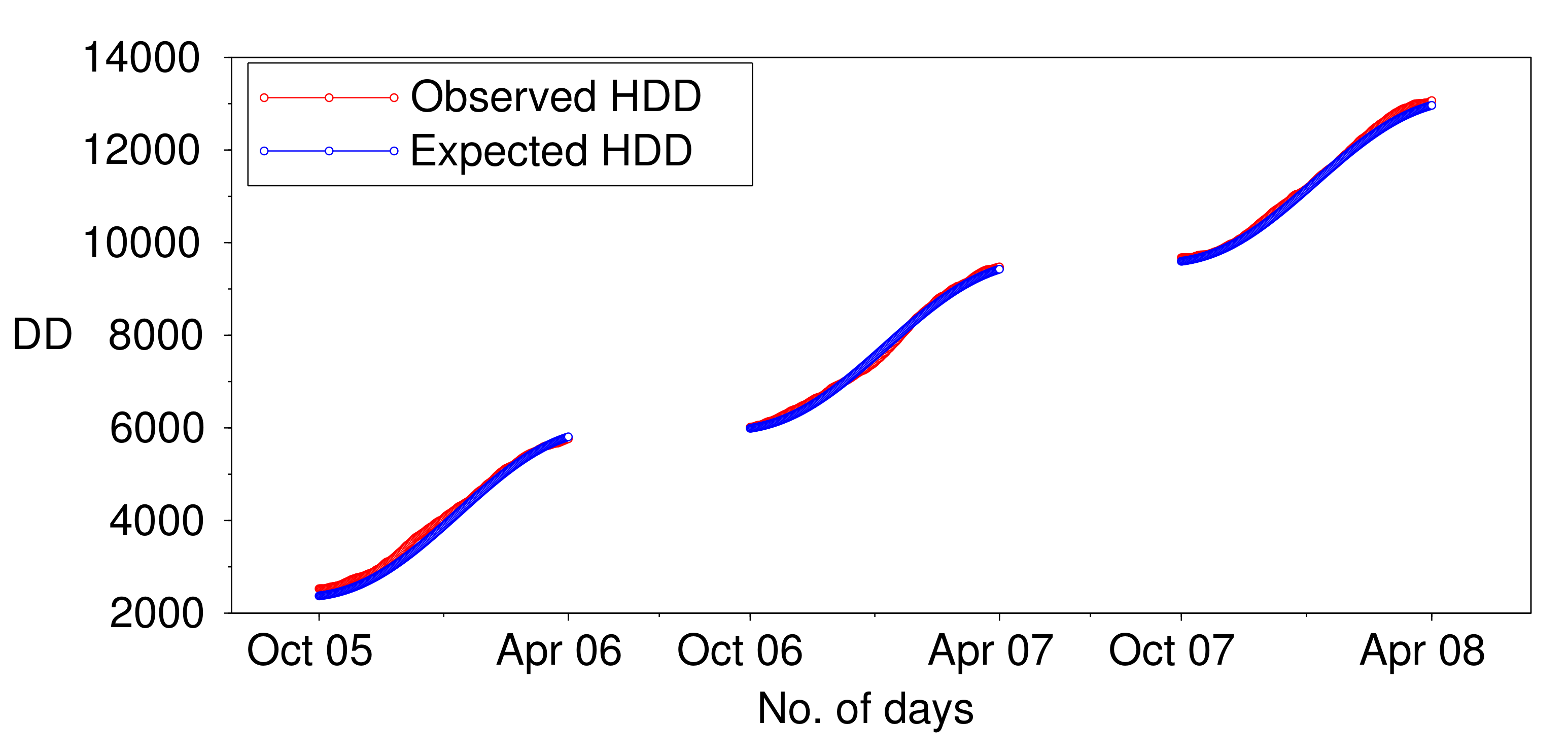
Remark 4.

As HDD/CDD indices depend on the number of days over which they are considered, and $max(x,0)\ge 0$ for any $x\in \mathbb{R}$, we deduce that

$$\mathrm{HDD}(n+1)=\sum _{j=1}^{n}max(B-T_j,0)+max(B-T_{n+1},0)\ge \mathrm{HDD}\left(n\right).$$

Similarly, $\mathrm{CDD}(n+1)\ge \mathrm{CDD}\left(n\right)$. Hence, HDD/CDD indices rise with increasing n.

For example, let us return to the results in Section 3.4 which are summarised in Figure 5. HDD months for Toronto at the CME are from January to April and from October to December. For the four-year period from January 2005 to December 2008 ($n=1461$), the HDD months would correspond to the periods October 2005–April 2006 ($274\le n\le 485$), October 2006–April 2007 ($639\le n\le 850$) and October 2007–April 2008 ($1004\le n\le 1216$). We calculate $\mathrm{HDD}\left(n\right)$ in (13) during these three periods. The results are shown in Figure 6. The data set $\{T_j:1\le j\le 1461\}$ was used to compute the observed HDD (red graph), while the data set $\{{\widehat{T}}_j:1\le j\le 1461\}$ was used to compute the expected HDD (blue graph). As anticipated, $\mathrm{HDD}(n+1)\ge \mathrm{HDD}\left(n\right)$.

4.2. Call Option Pricing: An Example

In this section, we illustrate how to use our stochastic harmonic oscillator temperature model to price a call option, where the underlying variable is the HDD index. Other types of options or trading strategies may also be considered.

Suppose that the contract period is from 1–31 December ($n=31$), the strike HDD is $K=550$, the tick size is $s=\$20$ and the risk-free rate is $r=0.0206$. The latter was determined from the 10-year Canadian government bond yields compiled by Bloomberg (see http://www.bloomberg.com/quote/GCAN10YR:IND, accessed on 12 October 2021).

The stochastic harmonic oscillator temperature model we use is

$$\begin{array}{cc}\hfill {\widehat{T}}_j& =\frac{\widehat{a}}{6.3^2}+\left({\widehat{\theta }}_1-\frac{\widehat{a}}{6.3^2}\right)cos\left(6.3t_j\right)+\frac{{\widehat{\theta }}_2}{6.3}sin\left(6.3t_j\right)\hfill \\ \hfill & +{\widehat{\sigma }}_1{\int }_0^{t_j}cos\left(6.3(t_j-u)\right)\mathrm{d}{W}_1\left(u\right)+\frac{{\widehat{\sigma }}_2}{6.3}{\int }_0^{t_j}sin\left(6.3(t_j-u)\right)\mathrm{d}{W}_2\left(u\right),\hfill \\ \hfill & j=1,2,\dots ,31,\hfill \end{array}$$

(14)

where the parameters $\widehat{a}$, ${\widehat{\theta }}_1$, ${\widehat{\theta }}_2$, ${\widehat{\sigma }}_1$ and ${\widehat{\sigma }}_2$ are as in (12), $t_j=(j-1)\mathrm{\Delta }t$ for $j=1,2,\dots ,31$ and

$$\mathrm{\Delta }t=\frac{1}{365}\frac{n}{n-1}=0.0028,t_{\max }=(n-1)\mathrm{\Delta }t=\frac{n}{365}=0.0849.$$

Note that $\{{\widehat{T}}_j:j=1,2,\dots ,31\}$ is a discretised sample path of the process T. Taking $B=18$, (13) gives the random variable

$$\mathrm{HDD}\left(31\right)=\mathrm{HDD}(31;\{{\widehat{T}}_j:j=1,2,\dots ,31\})=\sum _{j=1}^{31}max(18-{\widehat{T}}_j,0).$$

(15)

Using a risk-neutral framework, the price C of a call option is therefore

$$C=s{\mathrm{e}}^{-\frac{rn}{365}}E(max(\mathrm{HDD}\left(n\right)-K,0)).$$

(16)

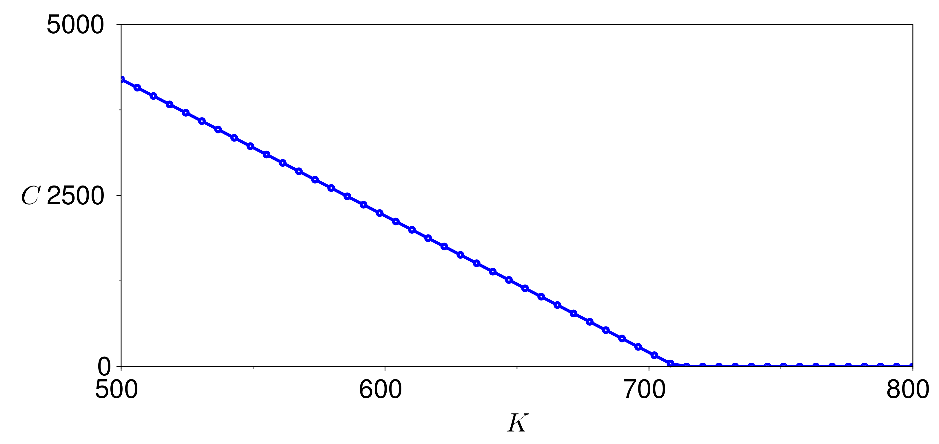
To evaluate the expectation in (16), we take the average of 5000 sample paths of the process (14) and substitute it into (15). The resulting call price is $C=\$3196.84$. Figure 7 shows the variation of the call price over a range of strike HDDs. The figure is generated by varying K in (16) from 500 to 800.

4.3. Sensitivity Analysis

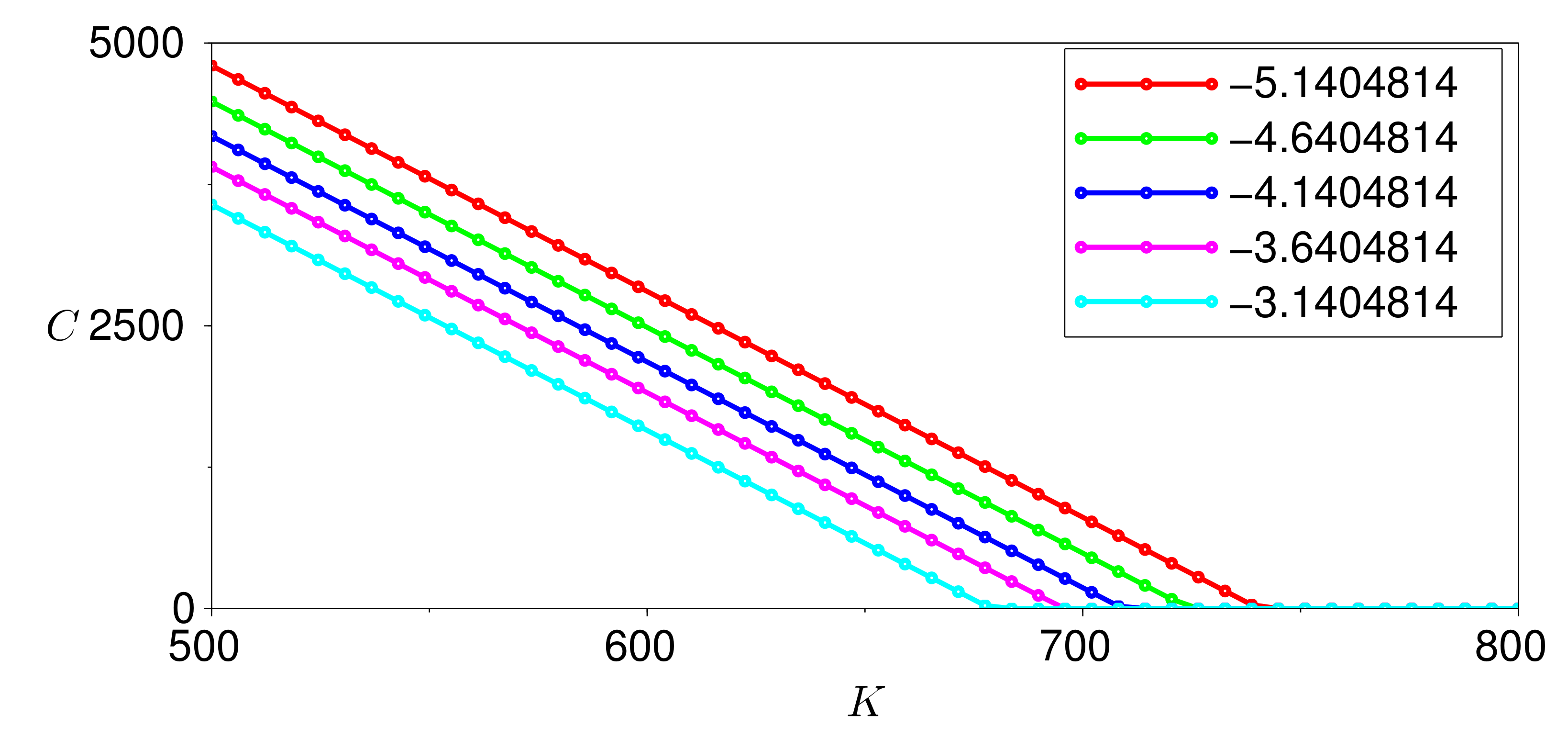
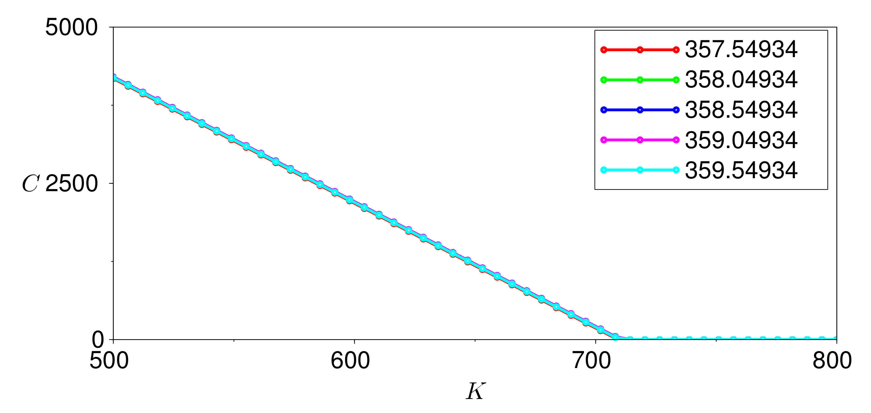
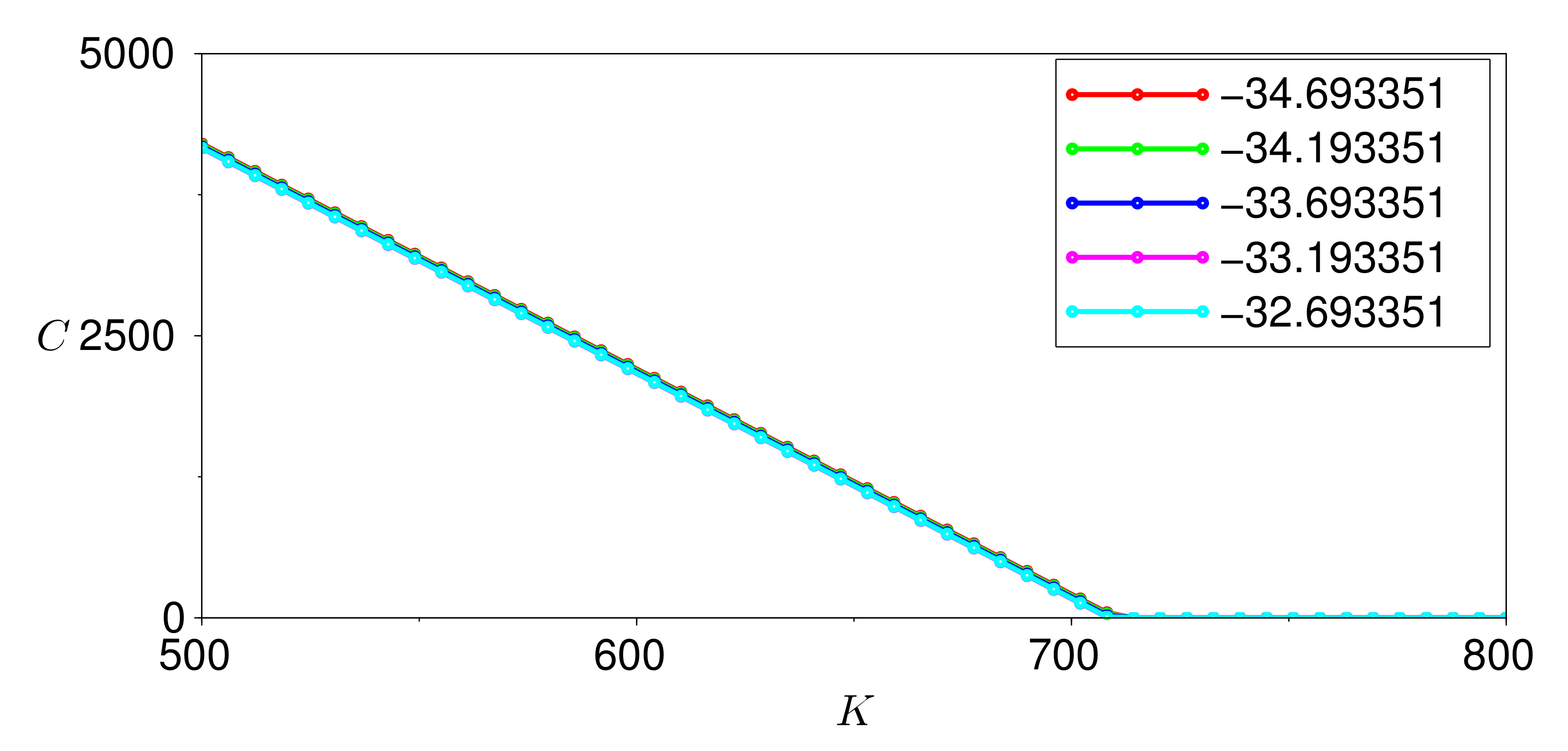
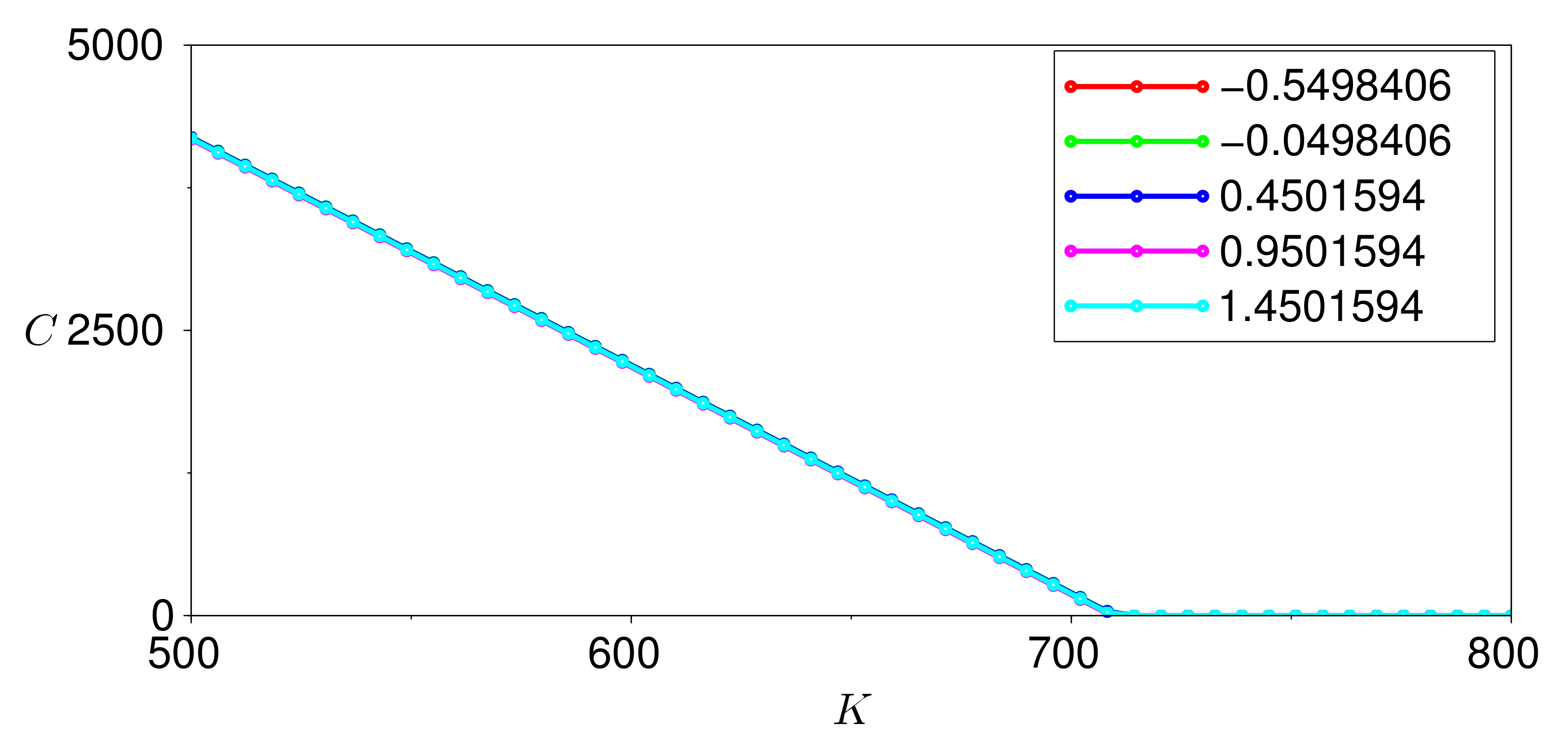
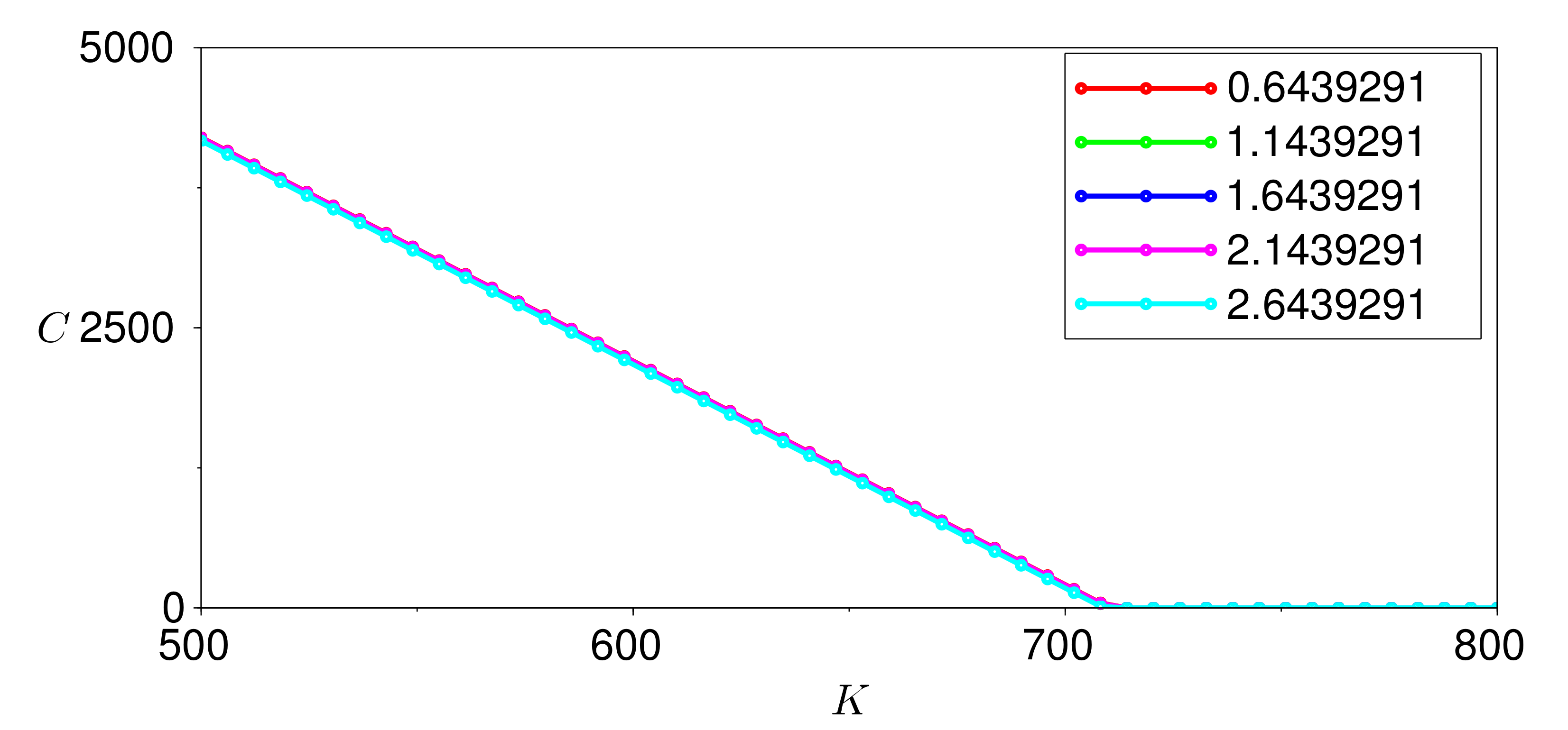
Following Siu et al. [23], we perform a sensitivity analysis for the call option price when the parameters of the model vary. The aim is to identify the key parameters that have significant impact on the call price.

To explain the methodology, let us suppose that we wish to investigate the sensitivity of C with respect to a by looking at how C behaves with respect to K as a is varied. More precisely, we assume that ${\widehat{\theta }}_1$, ${\widehat{\theta }}_2$, ${\widehat{\sigma }}_1$ and ${\widehat{\sigma }}_2$ are fixed as in (12) and let $\widehat{a}$ vary through five different values on an interval of unit radius centred at the value 358.88 of $\widehat{a}$ in (12). For each $\widehat{a}$ in this interval, we perform the calculations similar to those for Figure 7.

Figure 8 shows the impact of varying a, Figure 9 of varying ${\theta }_1$, Figure 10 of varying ${\theta }_2$, Figure 11 of varying ${\sigma }_1$ and Figure 12 of varying ${\theta }_2$. We conclude that the only parameter that has a significant effect on the call option price is ${\theta }_1=T\left(0\right)$. This result reveals that, under this stochastic harmonic oscillator temperature model, we must monitor the actual state of the temperature dynamics because of its considerable effect on the value of the weather-based option.

5. Conclusions

In this article, we proposed a new stochastic model for the temperature dynamics based on the classical harmonic oscillator (strictly speaking, a driven harmonic oscillator because of the term a in (1)). The temperature model is derived from a system of linear SDEs with two driving Wiener processes. We benchmarked our model by first using theoretical temperature data and then using actual temperature data observed at the Toronto Pearson International Airport. Substituting our temperature model in a temperature-based index such as HDD, we priced a call option under a risk-neutral framework and performed a sensitivity analysis. Numerical simulations suggest that the parameter related to the temperature at time zero was the only significant one that affected the call price as the strike HDD was varied. Of course, other temperature-based indices such as CDD or CAT can also be used, as well as other trading strategies besides a call option can also be considered following a similar procedure.

An extension of this model that is being currently investigated is a stochastic harmonic oscillator model with damping. The motivation behind this is the consideration of a temperature model that incorporates the gradual increase in temperature (due to the exponential factor introduced by damping) brought about by global warming, for example. Another possible extension is the modification of the stochastic terms in (3), e.g., from ${\sigma }_j\mathrm{d}{W}_j\left(t\right)$ to ${\sigma }_j{X}_j\left(t\right)\mathrm{d}{W}_j\left(t\right)$ for $j=1,2$. The resulting system remains linear and therefore a similar analysis can be performed.