Abstract
The paper considers the model of a call center in the form of a multi-server queueing system with Poisson arrivals and an unlimited waiting area. In the model under consideration, incoming calls do not differ in terms of service conditions, requested service, and interarrival periods. It is assumed that an incoming call can use any free server and they are all identical in terms of capabilities and quality. The goal problem is to find the stationary distribution of the number of calls in the system for an arbitrary recurrent service. This will allow us to evaluate the performance measures of such systems and solve various optimization problems for them. Considering models with non-exponential service times provides solutions for a wide class of mathematical models, making the results more adequate for real call centers. The solution is based on the approximation of the given distribution function of the service time by the hyperexponential distribution function. Therefore, first, the problem of studying a system with hyperexponential service is solved using the matrix-geometric method. Further, on the basis of this result, an approximation of the stationary distribution of the number of calls in a multi-server system with an arbitrary distribution function of the service time is constructed. Various issues in the application of this approximation are considered, and its accuracy is analyzed based on comparison with the known analytical result for a particular case, as well as with the results of the simulation.
1. Introduction
One of the fastest-growing segments of the telecommunications market is the use of call centers. In this field, most of the costs of maintaining a call center are the salaries of employees who provide various kinds of information services to clients. The number of operators is chosen based on some standard measures, for example, the proportion of customers for which the waiting time for the start of service does not exceed the average time of the request servicing. The solution to the problem depends on the cost relationships between the components of the system. Therefore, the development of mathematical models and methods in this area is an necessary task. Traditional approaches of such studies lay in the field of queueing theory and related topics.
An excellent description of call centers and general issues in applying queueing models to studies were presented in [1]; some other general issues on the topic may be found in [2,3,4,5]. In this paper, we consider a call center model in the form of a multi-server queue with an incoming Poisson flow of calls, recurrent service, and an unlimited number of waiting places (). A number of articles by different authors are devoted to the study of models of this type, for example: [6,7,8,9,10]. Furthermore, there are studies of models with non-Poisson incoming flows, for example: [11,12,13,14,15,16,17,18]. The aforementioned works make it possible to obtain characteristics of the operation of the system mainly using numerical, approximate, or asymptotic methods. Moreover, most of the papers only evaluate mean values of waiting time or queue length, or the distribution of waiting time, or the distribution of queue length, but only under asymptotic conditions.
Our paper proposes one more approximate approach to solving the problem of studying the model, which allows one to obtain an accurate enough approximation of the probability distribution of the number of calls in the system for a wide class of service time distributions. Unlike other publications, our approach allows one to obtain a distribution of the number of calls, and this is performed directly without any asymptotic conditions, as in [8,16]. In addition, the proposed approach is based on substituting an approximation before performing the analysis instead of adapting known results for queues for the more general cases as was made in [9,10,12,14]. This allows us to obtain the final result in a simpler way with very high precision.
The main idea of the approach is in the approximation of the service time distribution by a two-phase hyperexponential one. The idea is taken from [19], where the problem of waiting time distribution was considered. We apply the idea to find the stationary distribution of the number of calls in this paper. For the model with hyperexponential service time, we use the matrix-geometric method to find the distribution of the number of calls in the system. To estimate the parameters of the hyperexponential distribution approximating a given distribution of the service times, in most cases, we use an approach based on three raw moments, which is in a certain sense similar to the results of [20]. However, for some cases, we have to use an approach based on two moments, and the results show us very high accuracy, even for such an approximation.
The only known exact analytical result is represented by the Pollaczek–Khinchine formula for a system with a single server [21,22]. In this paper, we compare the obtained approximation with this formula for the particular case in the model. For the other cases (when the number of servers ), we use the simulation results for the comparison. The performed numerical experiments prove the high accuracy of the approach for models in a wide class of service times.
The rest of the paper is organized as follows. In Section 2, we propose the mathematical model for the problem domain and formulate the goal of the study. In Section 3, we solve the problem for the partial case of the model with two-phase hyperexponential service times. To obtain the results for this case, we first derive the system of balance equation; after that, we apply the matrix-geometric method to solve it and derive the goal stationary probabilities at the end of the section. In Section 4, we propose a technique to obtain the results for the model ; also, we consider methods of the approximation and various issues of their applications. The results of estimating the accuracy of the proposed approach are presented in Section 5.
2. Mathematical Model
Consider a call center where we have several service devices (operators, servers) (Figure 1). An incoming call is redirected instantly to any free server or should be placed in a waiting queue if all the servers are busy. Calls in the queue are ordered according to the FCFS rule (First Come First Serve). After the completion of the service at any server, the server takes the first call from the queue for its service.
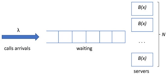
Figure 1.
Structure of the model.
Consider a model of the system in the following form. Let calls arrive at the system according to the stationary Poisson process with intensity , let there be an unlimited number of places for waiting calls, and also, let there be N operators (servers) working independently from each other with service times distributed with distribution function . For the goals of the study, we suppose that at least two finite raw moments exist for this distribution (the reasons may be found in Section 4).
Denote the stationary probabilities that we have exactly i calls in the system (both under the service and in the queue) by , . The goal of the study is to find this probability distribution. The condition of existence of the stationary regime is obvious and standard for such a class of models:
where is a rate of service in one server (the value that is inverse to the mean of a random variable with distribution function ).
The approach that we use is based on the approximation of the distribution by the hyperexponential distribution with two phases. So, we first try to obtain the solution for the model with hyperexponential service times. After that, we propose methods for the approximation of an arbitrary probability distribution by the hyperexponential one. At the end of the paper, we estimate errors of the solution of the original problem on the basis of comparison with known analytical results or simulation results.
The choice of hyperexponential distribution for the goals of the study is made based on the fact that this distribution allows studies to be carried out on queueing systems where it is used, and it can also approximate many other types of random variables distributions with a quite good accuracy.
3. Solution of the Problem for the Case of Hyperexponential Service Time
Let the service times be hyperexponentially distributed with the CDF:
where , , . Actually, this hyperexponential distribution is a mixture of two exponential distributions with parameters and chosen with probabilities and , respectively. So, actually, a server performs the service of a single call according to the exponential distribution with a chosen parameter. We name the servers that are currently working with parameter as working at the first phase, and the servers that are currently working with parameter as working at the second phase of the hyperexponential distribution.
Denote the number of servers that are working at the first phase in time moment t by and servers working at the second phase by . At any moment, the number of free servers equals . Furthermore, denote the number of calls in the queue in moment t by . Notice that it may be greater than zero only if .
Let us introduce the following notations for the stationary probabilities:
- for (when not all servers are busy),
- when all servers are busy. Here, and
So, the goal of the study for this model is to find these probabilities.
3.1. Balance Equations
We can construct the following system of the balance equations for the stationary regime. When the queue is empty, we have
for ; for the non-empty queue, we can write
for and .
We propose an algorithm for solving this system of equations with two stages. The first stage is based on the matrix-geometric method [23,24]. In this case, solution of part (5) of the system for will be expressed using term . This fact allows us to rewrite the rest of the system (2)–(4) in a closed form of the system of equations with the same number of variables. The second stage of the proposed algorithm will solve this system.
3.2. The First Stage: Matrix-Geometric Method
Denote the row vector
and vector to separate it from other components of the solution. Then, we can rewrite (5) in the matrix form:
where matrices and have the form
We write solution of system (6) in the matrix-geometric form:
Substituting it into (6), we derive a quadratic equation for the matrix :
This equation can be solved by the iterative method starting from zero matrix :
until absolute values of the entries of matrix become small enough.
To find vector , which is important for (7), we consider vector , whose entries can be written in the form
Denoting
we rewrite the system in the following form:
This is a system of linear equations with the same number of variables , for , and . Due to the fact that this system is a homogeneous, its non-trivial solution can be determined in a form with a constant multiplier which can be obtained from the normalization condition. In the next section, we propose an algorithm that reduces system (10)–(12) consisting of equations to the homogeneous system with equations with variables , that are entries of vector , which we wish to derive.
3.3. The Second Stage: Deriving Entries of Vector
Further, for the case , we can write corresponding equations from (11) in the form
where matrices with size , with size and with size have the following structures:
Finally, we write the last equations of system (10)–(12) in the form
where is a matrix with entries from (9).
From the first equation of the system, we can express:
where .
From the second equation, we express:
where .
Consider equality (18) for the case . We can write:
because . Let us substitute expression (19) into the last equation of system (17). Then we obtain the following equation for vector :
which is the homogeneous linear system for entries of vector . This system can be solved without any problems. So, we obtain vector .
After that, we can substitute vector as vector into the expressions
for , and find vectors iteratively for all .
Finally, applying expressions (7), we find vectors for all .
3.4. Stationary Probability Distribution of the Number of Calls in the System
As it is mentioned in Section 3.2, we obtained all vectors in the previous section, just in a form with a constant multiplier. To find true values of the vectors, we should apply the normalization condition
where are column vectors consisting of ones.
Denote stationary probabilities:
Here, means the probability that n servers are busy, and means that all N servers are busy and there are exactly i calls waiting in the queue.
4. Approximation for the Case of Arbitrary Distributed Service Times
Consider the system shown in Figure 1 with i.i.d. service times with arbitrary distribution function . To approximate probabilities from (25), we use expressions (23)–(24), supposing that distribution can be approximated by the hyperexponential distribution in form (1). So, the problem is reduced to establishing parameters , , , and that provide enough accuracy for the approximation of distribution by the hyperexponential distribution (1).
It is not hard to obtain the expressions for the parameters of the two-phase hyperexponential approximation if we have two or three finite raw moments of the original distribution . These expressions are presented in the following subsections.
4.1. Estimating Parameters of Hyperexponential Approximation Basing on Two Moments
Suppose distribution has two finite raw moments that we denote as and , respectively. We may estimate parameters , , , and from the following equalities for the moments:
The following expressions may be derived by an easy method:
4.2. Estimating Parameters of Hyperexponential Approximation Basing on Three Moments
If we suppose that distribution has three finite raw moments that we denote as , , and , respectively, then the parameters of the hyperexponential distribution can be derived as the solution of the following system of equations:
It is clear that the approximation based on three moments is more accurate than one based on two moments. Therefore, it should be preferable if it is possible.
4.3. How to Apply the Approximations
Actually, estimation of the parameters in such a way may lead us to the following several types of results, including some unusual cases:
- (1)
- , , , .
- (2)
- , , , .
- (3)
- Pairs and are complex numbers with their conjugates where all real parts are positive.
- (4)
- One of parameters or has a negative value of its real part.
Obviously, in the cases 2 and 3, such values cannot be values of the parameters of hyperexponential distribution (1), but in the next section, we show that these values may be applied for approximation (25) and the result will have enough good accuracy. Moreover, when we deal with the third case with complex values of the parameters, corresponding function (1) is not a distribution function, but approximation (25) still works.
If you meet case 4, it is better to use estimation scheme (27) using two moments, and . This excludes the possibility of obtaining negative values for parameters and .
5. Accuracy of the Obtained Approximation
The analytical result for the single-server queue is well known and it is expressed by the Pollaczek–Khinchine formula. Unfortunately, we cannot compare obtained approximation (25) with the Pollaczek–Khinchine formula analytically, but we can compare the results numerically by performing evaluations on the basis of analytical expressions. For the case of a multi-server queue, there are no exact analytical results in the literature, so we compare obtained approximation (25) with the results of the simulation.
Consider single-server queueing system . According to the Pollaczek–Khinchine formula, the characteristic function of the number of calls in the system has the form
Here,
is the Laplace–Stieltjes transform of distribution function of service time. Applying the inverse Fourier transform
we obtain probability distribution of the number of calls in the system.
We determine the accuracy of approximation (25) by using the Kolmogorov distance for discrete distributions
For the numerical experiment, we take the following three types of distribution functions with mean :
- (1)
- Gamma distribution with shape parameter and inverse scale parameter . The raw moments of the distribution are evaluated as follows:
- (2)
- Weibull distribution with parameters and , and with the raw moments
- (3)
- Lognormal distribution with parameters and . Its raw moments are the following:
Consider single-server systems with the Poisson arrival process with intensity and service times with distribution functions from the list above. The results of estimation parameters of hyperexponential approximation (1) using expressions (29) and (30) for these distribution functions and corresponding values of Kolmogorov distance (33) (line ) for the resulting approximation (25) are presented in Table 1, Table 2 and Table 3. Here, we compare distribution (25) with analytical results obtained using the Pollaczek–Khinchine formula (31) and (32). For the lognormal distribution in interval , applying formulas (29) and (30) leads to the case ; therefore, we use estimation expressions (28) for this interval. The corresponding results are presented in Table 4. Furthermore, we cannot obtain the result in the case of gamma distribution with shape parameter . We think that this case can be resolved directly, but it requires additional study.

Table 1.
Values of parameters , , and q of the hyperexponential approximation obtained for gamma distribution function for various values of its shape parameter , and corresponding Kolmogorov distances for the main result.
Table 2.
Values of parameters , , and q of the hyperexponential approximation obtained for Weibull distribution function for various values of its parameter , and corresponding Kolmogorov distances for the main result.
Table 3.
Values of parameters , , and q of the hyperexponential approximation obtained for lognormal distribution function for various values of its parameter (except values ), and corresponding Kolmogorov distances for the main result.
Table 4.
Values of parameters , , and q of the hyperexponential approximation obtained for lognormal distribution function for values of its parameter , and corresponding Kolmogorov distances for the main result.
In line of the tables, you may find the Kolmogorov distance for distribution (25) evaluated on the basis of hyperexponential approximations of service time distribution for the system with five servers (the intensity of the Poisson arrivals is taken equal to 4). The results are compared with the simulation results (note that the simulation results in the experiments are obtained with an error of 0.002 in terms of the Kolmogorov distance). All numerical evaluations for the examples are made using MathCAD software.
In Figure 2, you may find probability mass functions (PMFs) for some of the considered examples for the multi-server model with five servers. We chose the most interesting and the most “strange” cases of the approximation to use as examples.
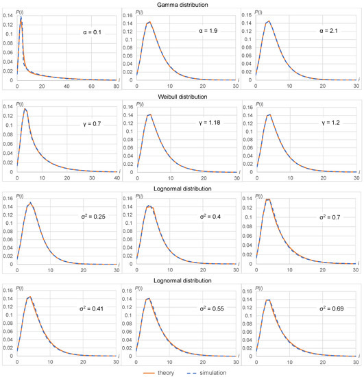
Figure 2.
PMFs obtained by the approximation and simulation for multi-server queue with various distributions of service time and their parameters.
As we see from the presented results, distribution (25), using hyperexponential approximation of the service time, has very high accuracy in almost all cases (the worst results are only obtained for gamma distribution with a small value of the shape parameter). You may find various values of the parameters of the hyperexponential approximation in Table 1, Table 2, Table 3 and Table 4, including strange ones (complex values, ), but the final result (25) works properly for these cases too.
6. Discussion
The study presented in the paper shows that a two-phase hyperexponential approximation can be applied for service time distribution in the queue. This approximation provides highly accurate results for the goal probability distribution of the number of calls in the system even in cases where the approximation cannot be used as a distribution function. A comparison of the results with analytical results for the case of a single-server queue and simulation results for the case of a multi-server queue show the high accuracy of the approach.
Furthermore, in the paper, the analytical result for the system with hyperexponential service time is derived on the basis of the matrix-geometric approach. The result can be used both directly for the analysis of the queues or together with the hyperexponential approximation of the service time distribution for the analysis of the queues.
We believe that hyperexponential approximation can be applied in studies that investigate other types of queueing models where it can allow one to obtain a solution of a problem or, at least, obtain it more easily than by other methods. For example, we see good possibilities in analyzing systems of and types using the approximation and approach proposed in the paper.
Author Contributions
Conceptualization, A.N.; methodology, A.N.; software, A.M.; validation, A.M. and S.M.; formal analysis, S.M.; investigation, A.N.; writing—original draft preparation, A.N. and S.M.; writing—review and editing, A.M.; visualization, A.M.; supervision, A.M. All authors have read and agreed to the published version of the manuscript.
Funding
This research received no external funding.
Institutional Review Board Statement
Not applicable.
Informed Consent Statement
Not applicable.
Conflicts of Interest
The authors declare no conflict of interest.
References
- Gans, N.; Koole, G.; Mandelbaum, A. Telephone Call-centers: Tutorial, Review and Research Prospects. Manuf. Serv. Manag. 2003, 5, 79–141. [Google Scholar] [CrossRef] [Green Version]
- Koole, G.; Mandelbaum, A. Queueing Models of Call Centers: An Introduction. Ann. Oper. Res. 2002, 113, 41–59. [Google Scholar] [CrossRef]
- Borst, S.; Mandelbaum, A.; Reiman, M.I. Dimensioning large call centers. Oper. Res. 2004, 52, 17–34. [Google Scholar] [CrossRef]
- Stolletz, R.; Helber, S. Performance analysis of an inbound call center with skills-based routing. OR Spectr. 2004, 26, 331–352. [Google Scholar] [CrossRef]
- Stepanov, S.N.; Stepanov, M.S. Construction and analysis of a generalized contact center model. Autom. Remote Control 2014, 75, 1936–1947. [Google Scholar] [CrossRef]
- Nozaki, S.A.; Ross, S.M. Approximations in finite-capacity multi-server queues with Poisson arrivals. J. Appl. Prob. 1978, 15, 826–834. [Google Scholar] [CrossRef] [Green Version]
- Boxma, O.J.; Cohen, J.W.; Huffels, N. Approximations of the mean waiting time in an M/G/s queueing system. Oper. Res. 1979, 27, 1115–1127. [Google Scholar] [CrossRef]
- Whitt, W. Comparison conjectures about the M/G/s queue. OR Lett. 1983, 2, 203–209. [Google Scholar] [CrossRef]
- Kimura, T. Diffusion approximation for an M/G/m queue. Oper. Res. 1983, 31, 304–321. [Google Scholar] [CrossRef]
- Lisovskaya, E.Y.; Moiseeva, S.P. Study of the Queuing Systems M/GI/N/∞. Commun. Comput. Inf. Sci. 2015, 564, 175–185. [Google Scholar]
- Whitt, W. The effect of variability in the GI/G/s queue. J. Appl. Prob. 1980, 17, 1062–1071. [Google Scholar] [CrossRef]
- Shore, H. Simple Approximations for the GI/G/c Queue-I: The Steady-State Probabilities. J. Oper. Res. Soc. 1988, 39, 279–284. [Google Scholar]
- Whitt, W. Approximations for the GI/G/m queue. Prod. Oper. Manag. 1993, 2, 114–161. [Google Scholar] [CrossRef]
- Kimura, T. Approximations for multi-server queues: System interpolations. Queueing Syst. 1994, 17, 347–382. [Google Scholar] [CrossRef]
- Escobar, M.; Odoni, A.; Roth, E. Approximate solution for multi-server queueing systems with Erlangian service times. Comput. Oper. Res. 2002, 29, 1353–1374. [Google Scholar] [CrossRef]
- Whitt, W. A diffusion approximation for the G/GI/n/m queue. Oper. Res. 2004, 52, 922–941. [Google Scholar] [CrossRef] [Green Version]
- Sun, B.; Dudin, A.N. The MAP/PH/N multi-server queuing system with broadcasting service discipline and server heating. Aut. Control Comp. Sci. 2013, 47, 173–182. [Google Scholar] [CrossRef]
- Brandwajn, A.; Begin, T. Preliminary Results on a Simple Approach to G/G/c-Like Queues. In Proceedings of the International Conference on Analytical and Stochastic Modeling Techniques and Applications, Madrid, Spain, 9–12 June 2009; Al-Begain, K., Fiems, D., Horváth, G., Eds.; Springer: Berlin/Heidelberg, Germany, 2009; pp. 159–173. [Google Scholar]
- Ryzhikov, Y.I. Three methods for computing time characteristics of open queueing systems. Autom. Remote Control 1993, 54, 283–289. [Google Scholar]
- Gupta, V.; Harchol-Balter, M.; Dai, J.G.; Zwart, B. On the inapproximability of M/G/K: Why two moments of job size distribution are not enough. Queueing Syst. 2010, 64, 5–48. [Google Scholar] [CrossRef] [Green Version]
- Pollaczek, F. Über eine Aufgabe der Wahrscheinlichkeitstheorie. Math. Z. 1930, 32, 64–100. [Google Scholar] [CrossRef]
- Khintchine, A.Y. Mathematical theory of a stationary queue. Mat. Sb. 1932, 39, 73–84. [Google Scholar]
- Neuts, M.F. Matrix-Geometric Solutions in Stochastic Models; Johns Hopkins University Press: Baltimore, MD, USA, 1981; p. 352. [Google Scholar]
- Neuts, M.F. Matrix-analytic methods in queuing theory. Eur. J. Oper. Res. 1984, 15, 2–12. [Google Scholar] [CrossRef]
Publisher’s Note: MDPI stays neutral with regard to jurisdictional claims in published maps and institutional affiliations. |
© 2021 by the authors. Licensee MDPI, Basel, Switzerland. This article is an open access article distributed under the terms and conditions of the Creative Commons Attribution (CC BY) license (https://creativecommons.org/licenses/by/4.0/).