Abstract
Peridynamics (PD) is a novel nonlocal theory of continuum mechanics capable of describing crack formation and propagation without defining any fracture rules in advance. In this study, a multi-grid bond-based dual-horizon peridynamics (DH-PD) model is presented, which includes varying horizon sizes and can avoid spurious wave reflections. This model incorporates the volume correction, surface correction, and a technique of nonuniformity discretization to improve calculation accuracy and efficiency. Two benchmark problems are simulated to verify the reliability of the proposed model with the effect of the volume correction and surface correction on the computational accuracy confirmed. Two numerical examples, the fracture of an L-shaped concrete specimen and the mixed damage of a double-edged notched specimen, are simulated and analyzed. The simulation results are compared against experimental data, the numerical solution of a traditional PD model, and the output from a finite element model. The comparisons verify the calculation accuracy of the corrected DH-PD model and its advantages over some other models like the traditional PD model.
1. Introduction
Material fracture is a classical problem in solid mechanics [1]. In contrast to experimental research, numerical simulations provide a more efficient approach to understanding material fractures since they eliminate the limitations of complex specimen preparation, test environment conditions, and loading systems. The finite element method (FEM) is one of the commonly used numerical methods for solving fracture problems [2,3]. However, the crack-induced spatial discontinuities are not compatible with the partial differential equations in classical FEM models [4]. To deal with this problem, some remeshing techniques were incorporated into FEM models, which were usually cumbersome and time consuming [5,6]. Recently, the extended finite element method (XFEM) was proposed to solve the intermittent problems of cracks, holes, and inclusions by introducing additional nodal degrees of freedom and local strengthening functions [7,8]. Besides, the element erosion technique [9,10] and the phase field method [11,12] were proposed to simulate the problems of crack propagation with different levels of success. However, these methods are not applicable to simulate complex multi-crack extended penetration problems in three dimensions [13].
In recent years, meshless methods have been developed and applied in various engineering fields. They can simulate complex discontinuity without the remeshing process. For example, Cheng and Li [14] proposed a complex variable meshless method for fracture problems. Gao and Cheng [15] developed a meshless manifold method based on the complex variable moving least-squares approximation and the finite cover theory for fracture problems. Khazal et al. [16] presented an extended element free Galerkin method (XEFGM) for fracture analysis of functionally graded materials. In addition, the discrete element method (DEM) is suitable for simulating crack formation and propagation based on the discontinuity assumption. For instance, Kou et al. [17] adopted the DEM to investigate the dynamic crack propagation and branching in brittle solids. Owayo et al. [18] investigated the formation and propagation of cracks in cement-based materials via DEM simulations. Although some promising achievements have been obtained through the above researches, DEM has limitations when describing the mechanical behavior of the continuous material.
More recently, Silling et al. [19,20] proposed a new nonlocal theory of continuum mechanics called peridynamics (PD) for solving material fracture problems. It describes such a phenomenon by means of the failure of bonds linking material points. This method replaces the differential form of traditional balance equations with an integral form to avoid the singularity problem arising from the derivations at discontinuities. Therefore, PD is appropriate to describe the crack propagation in a unified framework. Owing to these advantages, it has been successfully applied to crack propagation problems [21,22], composite material damage [23,24], fluid mechanics and acoustics [25], and heat conduction analysis [26,27] etc. There are several kinds of peridynamics, such as bond-based PD [19], state-based PD [28], and element-based PD [29] etc., and they can be easily coupled with other numerical methods to deal with the interaction between different materials, such as PD-FEM [30], PD-SPH [31], and PD-DEM [32].
In traditional PD, the problem domain should be discretized into a series of particles with the same size and uniform distribution, thus limiting its application to complex problems such as multiscale analysis, multi-material problems, and adaptive analysis. Dipasquale et al. [33] proposed an adaptive refinement-coarsening method and applied it to a one-dimensional elastic wave propagation simulation. However, the problem of spurious stress waves was not completely solved in this model. Bobaru et al. [34] introduced adaptive refinement algorithms for peridynamics to deal with static and dynamic elasticity problems in 1D. Shojaei et al. [35] proposed an adaptive refinement strategy to use a variable grid size in a peridynamic model, which was verified to be effective and efficient. This approach was then successfully applied to simulate the fracture of a ceramic disk under central thermal shock [36]. Ren et al. [37,38] proposed a dual-horizon peridynamics (DH-PD) model incorporating non-uniform particle distribution and variable horizons to completely solve the problem of spurious stress waves. Wang et al. [39] derived state-based DH-PD governing equations using the Euler-Lagrange description, and they analyzed the dispersion characteristics of the model.
In this study, a particle volume correction and a surface correction are introduced in the DH-PD model to improve the calculation accuracy. In addition, the computational efficiency of this model is increased by incorporating a multi-grid technique. Two benchmark problems are simulated to verify the calculation accuracy of this model. Finally, this model is applied to analyze two numerical examples to validate the model’s reliability and applicability.
2. Peridynamics Theory
2.1. Traditional Peridynamics Theory
In traditional PD, the object occupying the spatial domain R is discretized into a series of closely arranged material points, as shown in Figure 1. The circular (spherical) region around the material point, x, with itself as the center point and δ as the radius is called the horizon, Hδ. The interaction force between the material point, x, with any other neighboring point, xʹ, in the horizon (xʹ ∈ Hδ) is called a pairwise force (bond). At any moment, t, the governing equation for any material point, x, is as follows [19]:
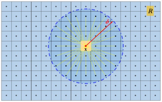
Figure 1.
Peridynamics model.
In Equation (1), f is the pairwise bond force between the material point x and its neighboring point xʹ, ρ is the density of the material, b is the body force vector, and u is the displacement vector. The integration domain, Hx, is the horizon of material point, x, in the reference configuration, mathematically, as . Additionally, δ is the radius of the nonlocal horizon of the material point, which is constant for each material point in the traditional PD theory. Finally, ξ = xʹ − x and η = uʹ − u denote the relative position vector and the relative displacement vector with neighboring particles in the reference configuration, respectively.
The key to building a PD model is to find an appropriate pairwise force function, f. Theoretically, any function that satisfies the linear admissibility condition and the angular admissibility condition can be a pairwise force function. In a bond-based PD model, the direction of the pairwise force vector is parallel to the displacement vector, ξ + η. For microelastic materials, the pairwise force function in PD model is given by
In Equation (2), c(δ) denotes the microelastic modulus, which can be derived from the strain energy equivalence principle, and expressed in terms of E and ν:
Additionally, s represents the bond stretch ratio between two material points, as defined by:
When s is greater than the critical elongation ratio, s0, of the material, the bond between these two points is considered to be broken, and the corresponding pairwise force disappears. The critical elongation ratio, s0, can be determined by the relationship given by Ren et al. [37]:
where Gc is the critical energy release rate of the material.
The variable μ in Equation (2) is a historical parameter describing whether the bond is broken. In this case, μ is defined as:
According to the above criterion for bond breakage, the degree of damage at the local material point, x, can be expressed as:
2.2. Dual-Horizon Peridynamics Theory
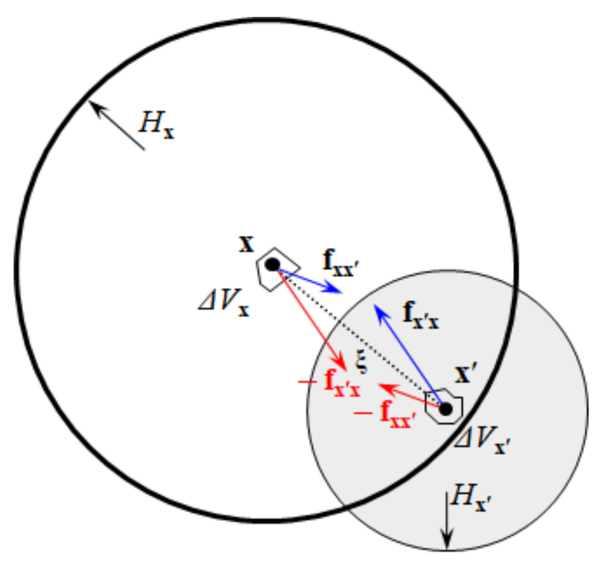
In traditional PD theory, the force acting on the particle x is the sum of the pairwise forces from all the neighboring particles in the horizon. Therefore, the horizon must be constant for all particles to ensure that the force always appears in pairs. If the horizons are variable, as shown in Figure 2, particle x is subjected to the force f(η, ξ) from the particle xʹ in its horizon. However, xʹ is not subjected to the force from x because its horizon does not include particle x. In this case, the existence of such an unbalanced force destroys the balance of linear momentum and angular momentum and results in ghost forces and spurious wave reflections during the simulation.
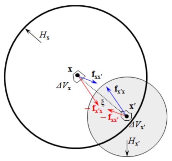
Figure 2.
Force vector in peridynamics with varying horizons.
Recently, Ren et al. [37] proposed the concept of dual-horizon, which can solve the spurious wave reflection problem. The dual-horizon is a union of points, the horizons of which include x. It is expressed, mathematically, as . The superscript prime of denotes a dual-horizon, and the subscript x denotes the object particle. Therefore, dual-horizon can be interpreted as a set of horizons that belong to particles that can include x in their horizons. In the DH-PD theory, a particle is subjected to two types of forces. The first one is the force from a neighboring particle in the horizon. The other one is the force from the particle in the dual-horizon. Furthermore, these two different types of forces are independent of each other, and the bond and dual bond can break independently in the fracture models.
In Figure 2, Hx is the horizon of particle x, where the bond xxʹ will exert a direct force fxxʹ on x, and xʹ will be subjected to the reaction force − fxxʹ according to Newton’s third law. Likewise, the dual bond xʹx will exert a direct force fxʹx on xʹ, and x will be subject to the reaction force − fxʹx. The time-dependent governing equations of DH-PD [40] are given as follows:
The micromodulus, c, in Equation (9) depends on the particle spacing of the material point x and is half of the corresponding micromodulus in traditional PD, see Equation (3).
3. DH-PD Numerical Method
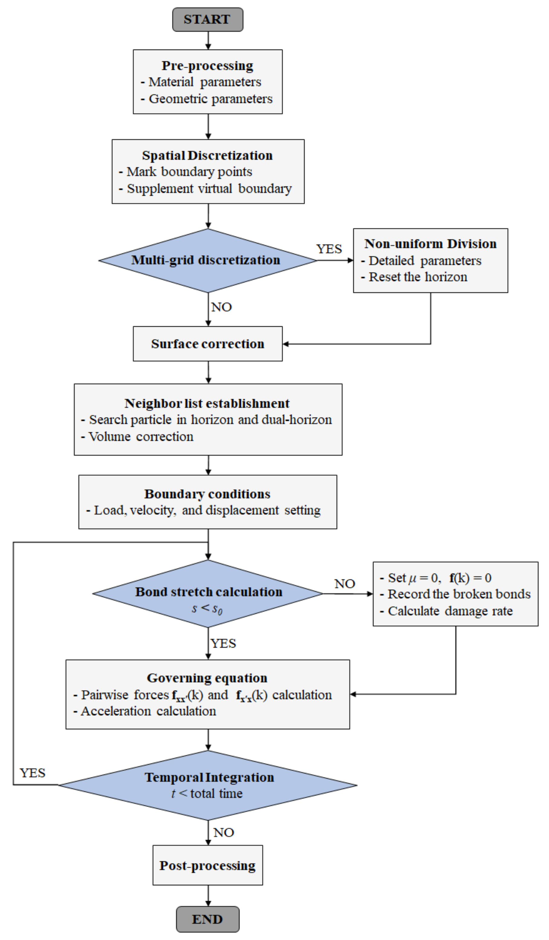
Figure 3 shows the program flowchart of the DH-PD model, which contains the pre-processing module, particle generation module, boundary treatment module, and damage degree calculation module. The C++ programming language is used to write the program code in this study.

Figure 3.
Program flowchart of the DH-PD model.
3.1. Non-Uniform Discretization
The problem domain in the PD model is discretized into a series of particles with the material information in the reference configuration. There are no elements or other geometrical connections between the particles. The size of each particle is uniformly arranged and contains a certain volume. The spatial information of each particle is characterized by the geometric center. Horizons of the particles in the DH-PD model are variable, so, finer discretization with smaller horizons is always used in the concerning region, such as the damage area. Additionally, the variability of the horizons requires coarser particles for the unimportant areas.
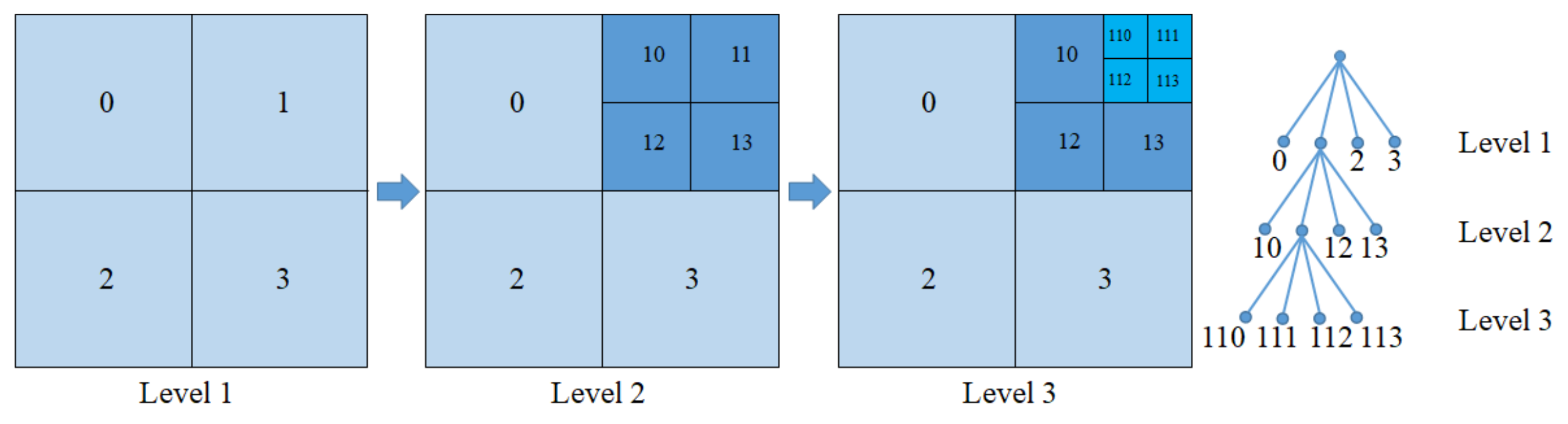
The discretization is carried out layer by layer. First, the domain is discretized into a series of coarse particles with the same spacing. Then, the second-level discretization is carried out in the area with high stress concentration. The coordinates of the second-level particles can be determined based on their geometric relationship with the first-level particles. For example, a two-dimensional plane consists of four particles (P0, P1, P2, P3) with a volume of V and a spacing of Δx, as shown in Figure 4. For the second-level discretization, a coarse particle (P1) with the coordinates (x1, y1) can be divided into four fine particles (P10, P11, P12, P13), with a volume of 0.25 V and a spacing of 0.5 Δx. Therefore, the coordinates of the fine particle P11 are (x1 + Δx/4, y1 + Δx/4). In the same way, the second-level particle (P11) can be divided into four third-level particles (P110, P111, P112, P113). The volume of the third-level particle is V/16, and the particle spacing is Δx/4. Based on this discretization, the coordinates of these finer particles can be easily determined by their geometrical relationships.
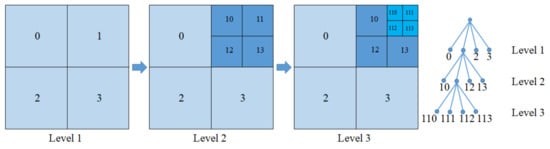
Figure 4.
Layer-by-layer discretization in DH-PD model.
It is worth noting that, when the size difference between adjacent particles is too big, the finer particles cannot include any coarse particles in their horizons, which may result in bond deficiency and lead to unexpected failure near the interface. Therefore, in the presented model, the size difference between adjacent particles is suggested to be smaller than the radius of the finer particle’s horizon.
3.2. Volume Correction and Surface Correction
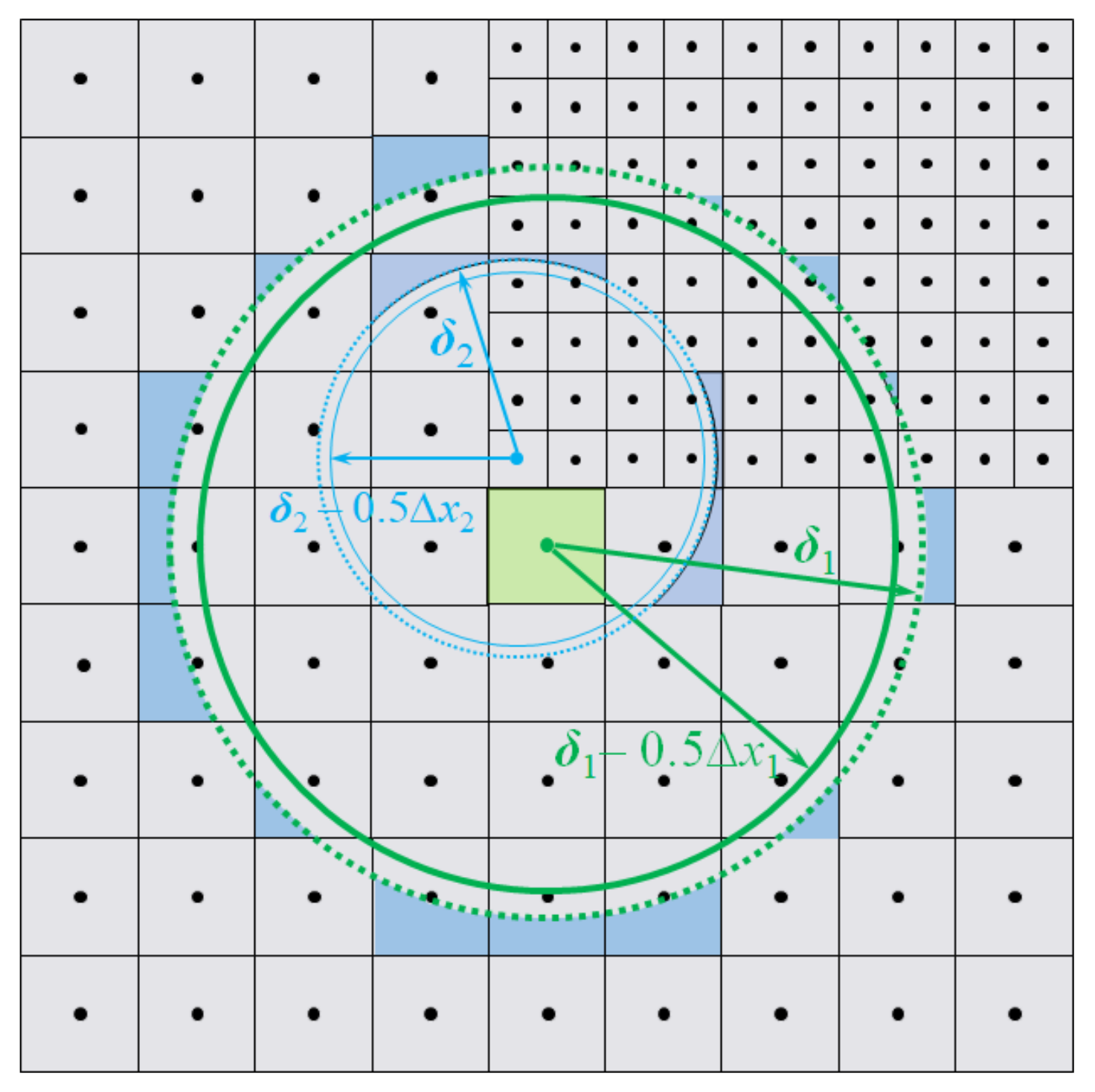
In PD theory, the problem domain is discretized into a series of particles, and each particle interacts with the neighboring particles in its horizon. However, some particles are located on the boundary and are not completely included in the horizon, as shown in Figure 5. Therefore, the model requires corrections with regards to the volumes of these particles when calculating the pairwise forces. For the multilevel discretization in DH-PD, the horizons of different particles vary with particle size, the particle volume can be corrected as:
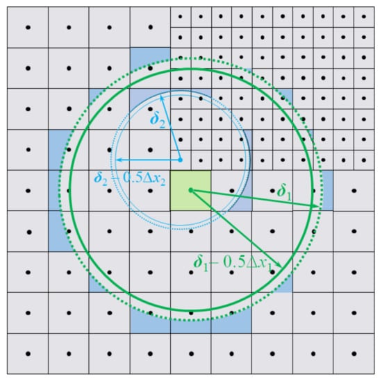
Figure 5.
Volume correction for the collocation points inside the horizon.
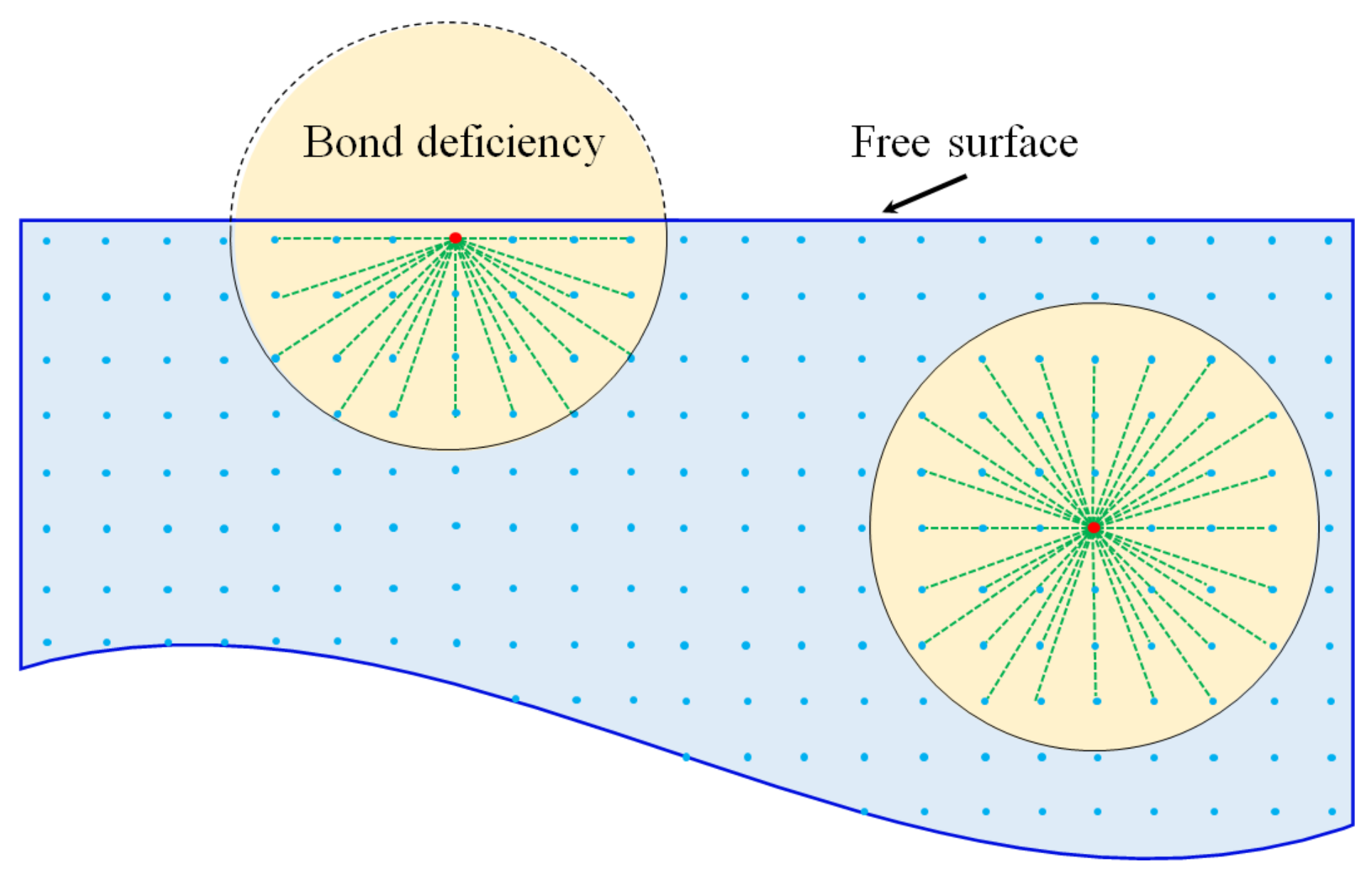
For the particles near the boundary of the problem domain, the number of neighboring particles in the horizon is lower than other particles, as shown in Figure 6. Therefore, the stiffness of the particles near the boundary is falsely reduced [41]. To deal with this problem, Scabbia et al. [42] presented an effective approach to mitigate the surface effect in state-based Peridynamics. Madenci and Oterkus [43] reconstructed the strain energy density near the boundary through the force density method and energy method to obtain the corresponding correction coefficients. The surface correction factor can be obtained by exerting a simple fictitious load to the object along the direction of the reference coordinate system. Based on this, the ratio of the strain energy densities calculated through the classical continuum mechanics theory and PD theory can be used as a valid surface correction factor.
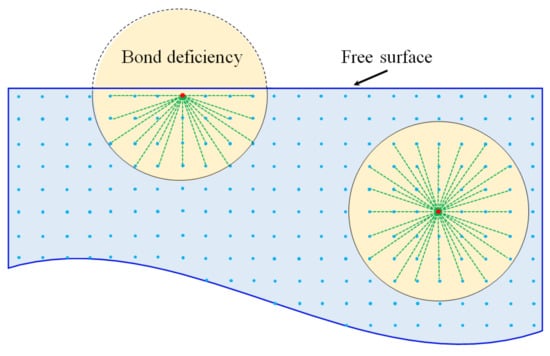
Figure 6.
Bond deficiency for the material points close to the free surfaces.
3.3. Explicit Time Integration
Explicit time integration is the simplest solution for the PD equations in dynamics simulations. In this method, acceleration and velocity are approximatively determined by the finite difference form of the displacement [44]:
In Equations (11) and (12), , , define the displacement, velocity, and acceleration vector, respectively. In addition, Δt represents the time increment, k denotes the particle number, and n equals the time step number. With this, displacement can be updated as:
Restricting the time step increment ensures the stability of the time integration, because the computational stability decreases as the time step increases. Silling and Askari [20] proposed a relationship,
to determine the critical time step in a PD model, where p is the number of the neighboring particles in the horizon, ΔVp is the volume of the neighboring particle, and Cp is the microelastic modulus of the material.
4. Numerical Examples and Discussions
In this section, two benchmark tests are simulated to verify the accuracy and stability of the corrected DH-PD model: longitudinal vibration of a bar and wave reflection in a rectangular plate. The numerical results are compared with the analytical solutions and the finite difference method (FDM) results to validate the computational accuracy and the feasibility of the non-uniform discretization. Then, the corrected DH-PD model simulates two numerical examples: fracture of an L-shaped concrete specimen and mixed damage of a double-edged notched (DEN) specimen. The applicability and unique advantages of this model in crack propagation modeling are discussed.
4.1. Benchmark Problem 1: Longitudinal Vibration of a Bar
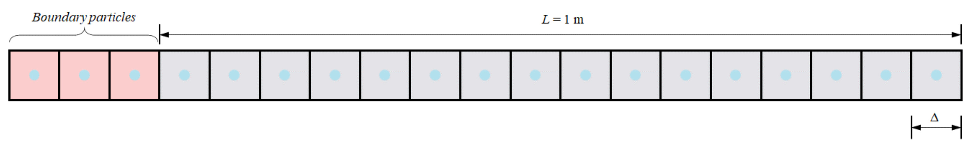
Figure 7 shows a bar with a fixed end on the left. The set parameters for the bar include the length of the bar, L = 1 m, the elastic modulus, E = 200 GPa, its Poisson’s ratio, ν = 0.33, and the density, ρ = 7850 kg/m3. The initial velocity of each material point is vx (x, t) = 0, and the initial displacement gradient is defined as:
where H is a step function, and ε = 0.001 is the initial strain.
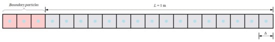
Figure 7.
Geometry of a bar and its discretization.
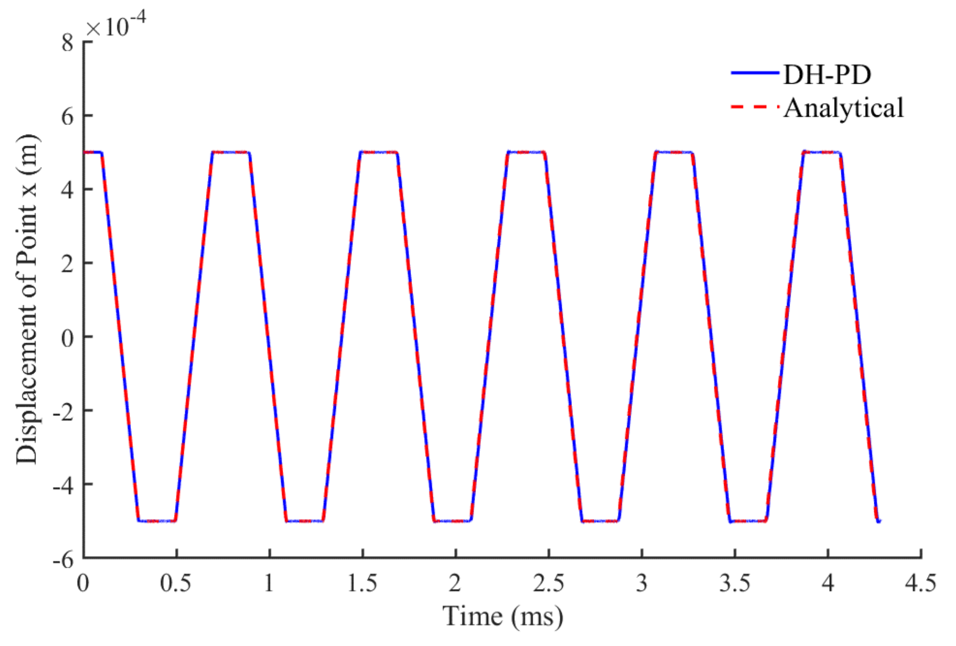
The bar is discretized into 1000 particles with a particle size of Δx = 0.001 m. Three fictitious boundary particles are fixed at the left side of the bar for the enforcement of displacement constraints. “No-fail zone” is commonly used for some applications under extreme loading conditions to avoid unexpected failure between the particles close to the external boundaries. For the loading conditions in the numerical examples presented in this paper, no-fail zone is not used. The computational time step is set as Δt = 0.2 μs, and the horizon associated with each particle is set as 3Δx. The particle with the initial position of x0 = 0.5 m is selected as the analysis object. Its displacement time history is compared with the analytical solution [44], as shown in Figure 8. The expected longitudinal vibration is successfully captured by the DH-PD model after the volume correction and surface correction. Overall, the numerical results are consistent with the analytical solution, thus verifying the accuracy of the presented DH-PD model.
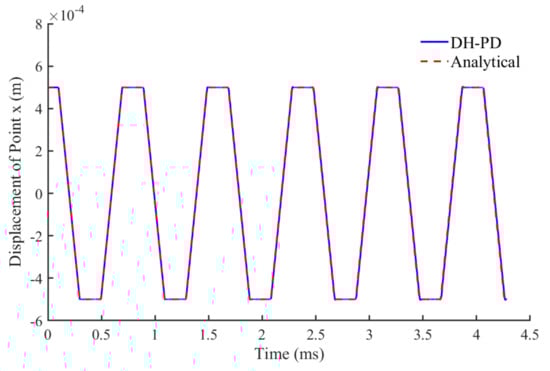
Figure 8.
Variation of the displacement of the particle numbered 500 with time.
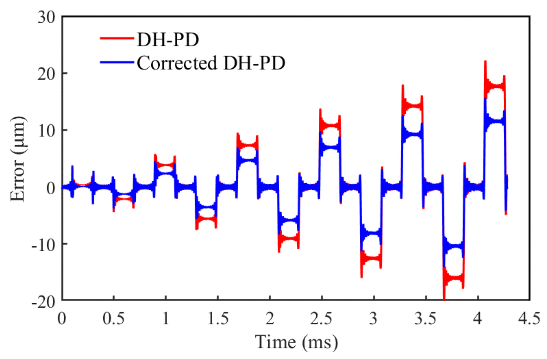
An error analysis is conducted, below, to assess the effect of the volume correction and surface correction on the calculation accuracy. The parameters are set (shown in Figure 9), and the analysis shows that the introduction of the volume correction and surface correction reduces the error to 0.01 mm.
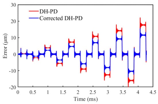
Figure 9.
Errors of the DH-PD model with and without correction.
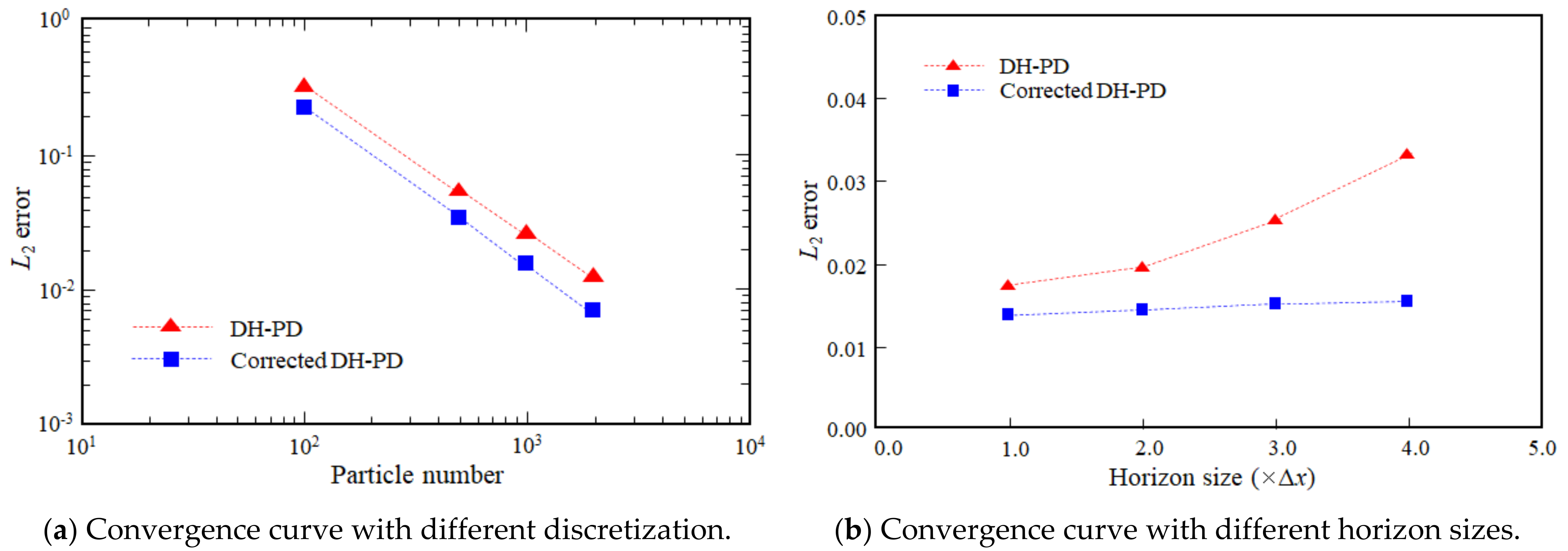
Figure 10 shows the convergence curves of DH-PD and corrected DH-PD models at t = 4.0 ms. It indicates that the L2 error in the displacement of the corrected DH-PD model is smaller than that of the DH-PD model, thus verifying that the volume correction and surface correction can improve the computational accuracy to some extent. Figure 10b shows that horizon size has little effect on the computational accuracy for the corrected DH-PH model in this case study. According to Silling and Askari [20], the horizon radius slightly greater than 3∆x usually works well. Therefore, the horizon radius is fixed at 3.015 times the particle size in this work.
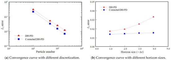
Figure 10.
Convergence curves in L2 error norm of DH-PD and corrected DH-PD models.
4.2. Benchmark Problem 2: Wave Reflection in a Rectangular Plate
Figure 11 shows the geometric size of a rectangular plate in the initial state of: length, L = 10 m, width, W = 1 m, elastic modulus, E = 10 GPa, density, ρ = 2500 kg/m3, and Poisson’s ratio, ν = 0.33. The left end of the plate is fixed, and the right end is assigned a velocity boundary, v(t), based on Equation (16). In Equation (16), H (t0 − t) is the Heaviside function, and t0 = 2 ms is the duration of the velocity boundary. The plate is dispersed into 1600 particles, and there is a dense area in the middle section of the plate with the following PD parameters: matter point dispersion spacing (Δx = 0.1 m), particle spacing in the encrypted region (0.5Δx), and the time step (Δt = 1 μs).
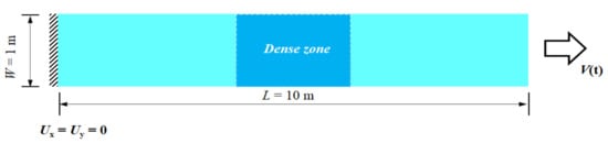
Figure 11.
Geometry of the plate in the initial state.
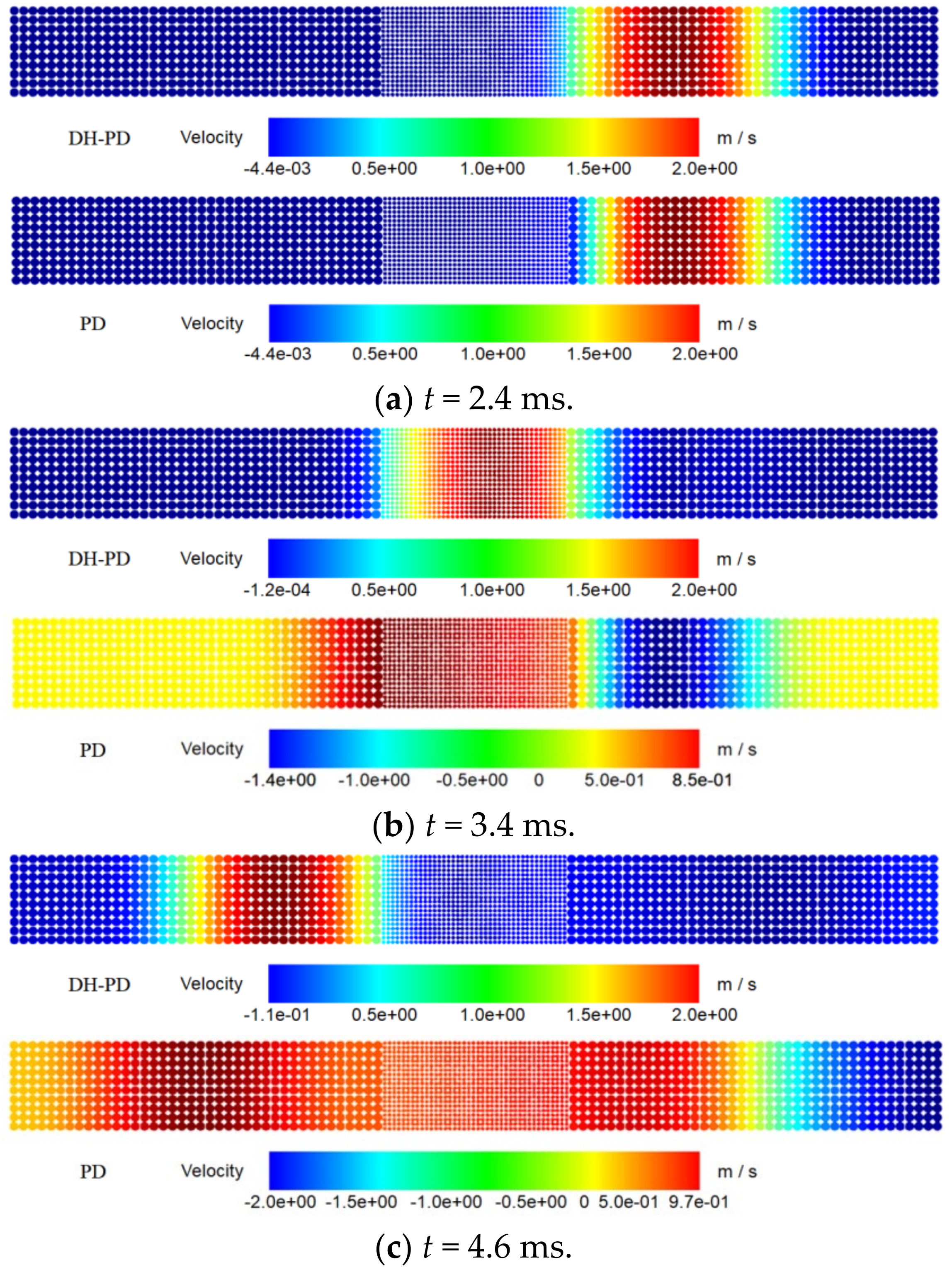
The numerical results of the velocity wave propagation through the dense zone are shown in Figure 12 (DH-PD above, PD below). When the time is 2.4 ms, the velocity waveform transmitted is about to enter the dense area. Figure 12a shows that both PD and DH-PD simulate this stage accurately. When the time is 3.4 ms, the velocity of the center point in the dense area reaches the theoretical maximum of 2 m/s when using the DH-PD algorithm. When the traditional PD algorithm is used, the phenomenon of false wave reflection to the right will be found, weakening the wave peak of the velocity waveform in the dense area (Figure 12b). This violates the wave propagation theory in the same material and cannot completely simulate the wave propagation process. When the time reaches 4.6 ms, the velocity wave leaves the dense area and enters the non-dense area (Figure 12c).
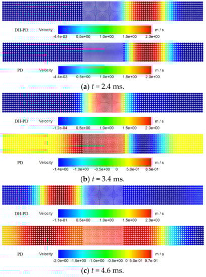
Figure 12.
Velocity contour of wave passing through dense area.
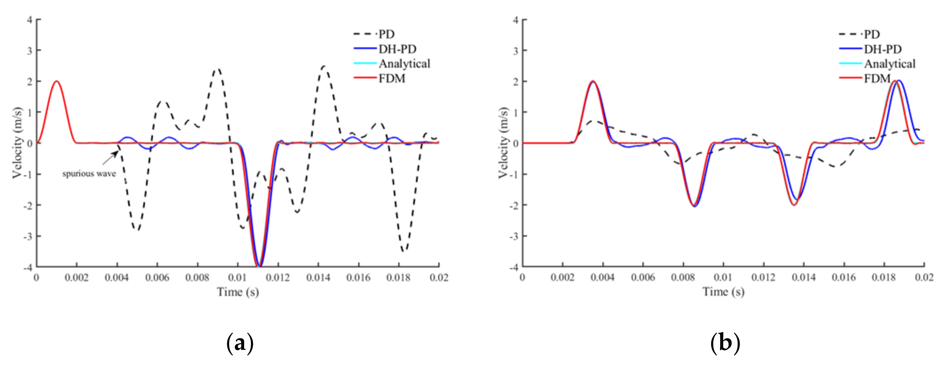
The material points at the free end of the plate and the middle-end of the plate are monitored and their velocity characteristics are extracted and shown in Figure 13. The FDM simulation curves are almost identical to the analytical solutions, both of which can be used as a reference group. The conventional PD simulation is used to show anomalous spurious reflected waves. At a time of 3.5 ms, the velocity in the dense region is less than 1 m/s, which is half of the real value, and the spurious velocity wave is also received at the free end. DH-PD can simulate the complete propagation process of the wave, and it matches both the analytical solution and the FDM solution.

Figure 13.
Time-velocity curves of analytical solution and numerical solution. (a) Velocity history at the free end of the bar. (b) Velocity history at the middle of the bar.
4.3. Numerical Application 1: Fracture of L-Shaped Concrete Specimen
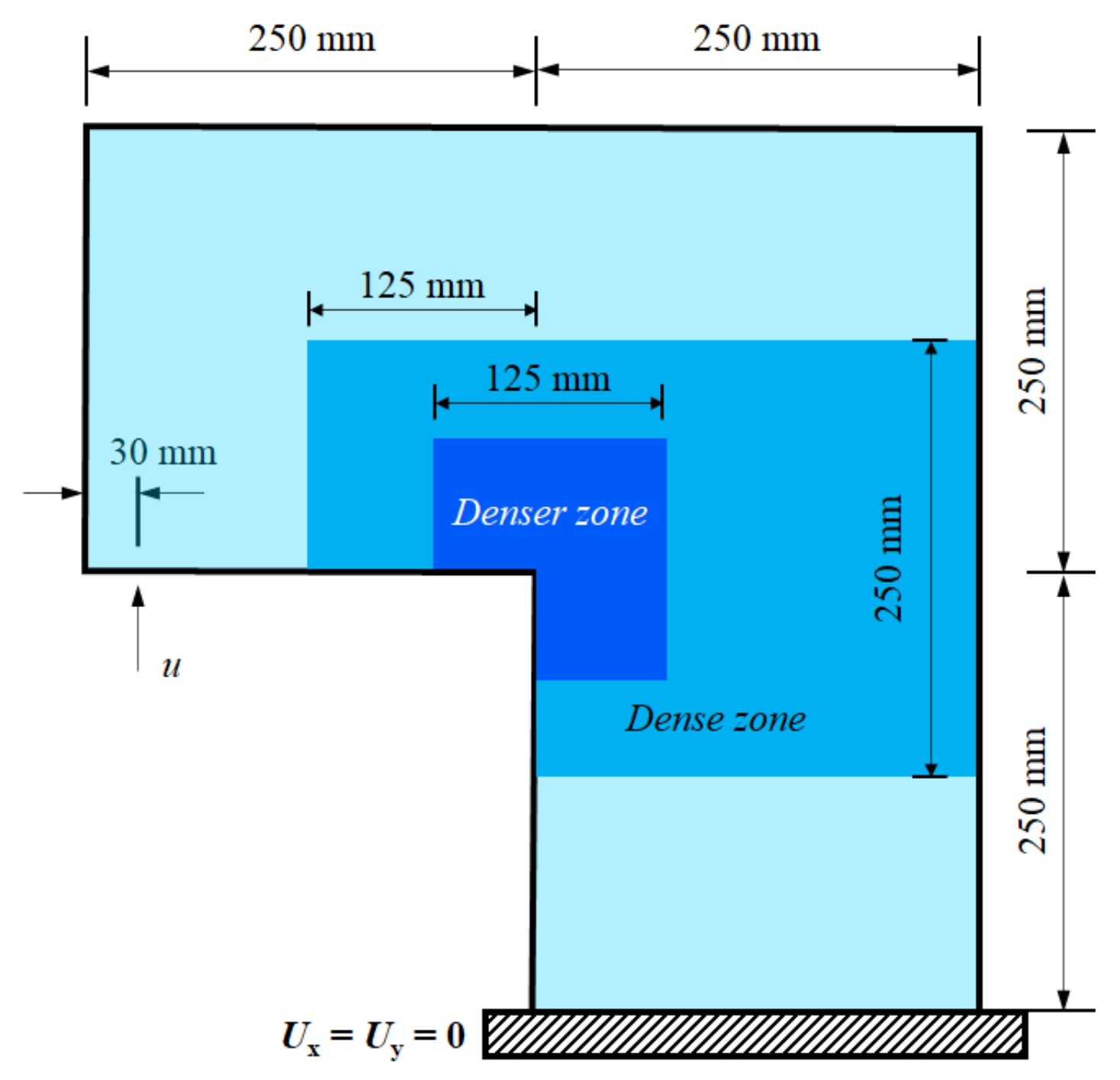
Figure 14 shows the geometry of an L-shaped concrete specimen [45,46]. A total of 22,728 particles with different particle sizes and varying horizons are used in this case. Specifically, 7504 finer particles (Δx = Δy = 1.25 mm) are used near the corner of the L-shaped specimen, where the stress is relatively concentrated, 4300 coarser particles (Δx = Δy = 5 mm) are distributed at the periphery of the specimen, and 10,924 particles of size Δx = Δy = 2.5 mm are distributed between finer particles and coarser particles. The horizon size is set as 3.015 times the particle spacing. The information of the particles is shown in Table 1 and Figure 14. The other physical parameters include the modulus of elasticity, E = 25.85 GPa, the Poisson’s ratio, ν = 0.18, the energy release rate, Gc = 65 J/m2, and the time increment, Δt = 0.1 μs. A displacement boundary, u, is exerted at the left side of the specimen, as shown in Figure 14.
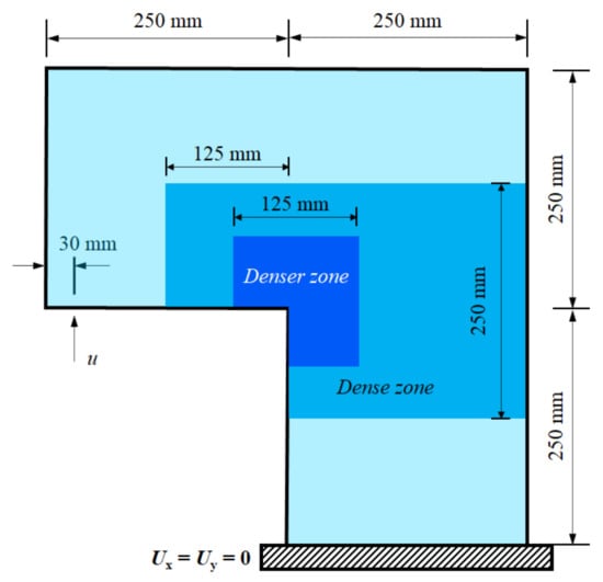
Figure 14.
L-shaped plate geometry and three-level discretization.

Table 1.
Values of peridynamics parameters for the DH-PD model.
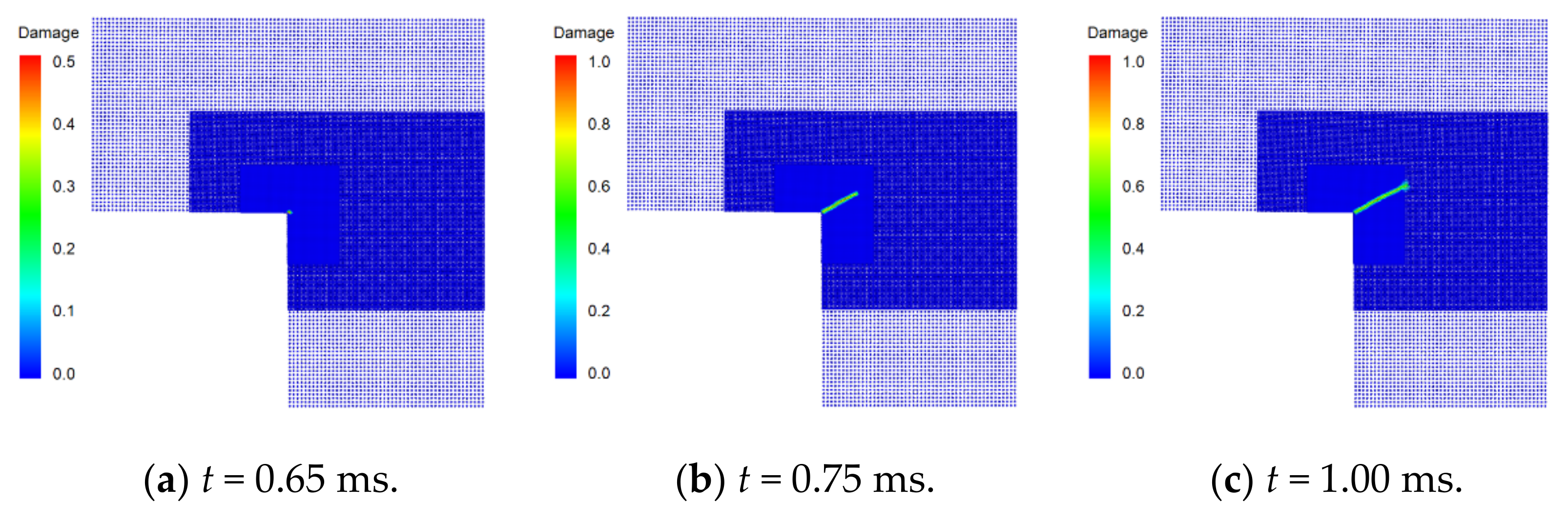
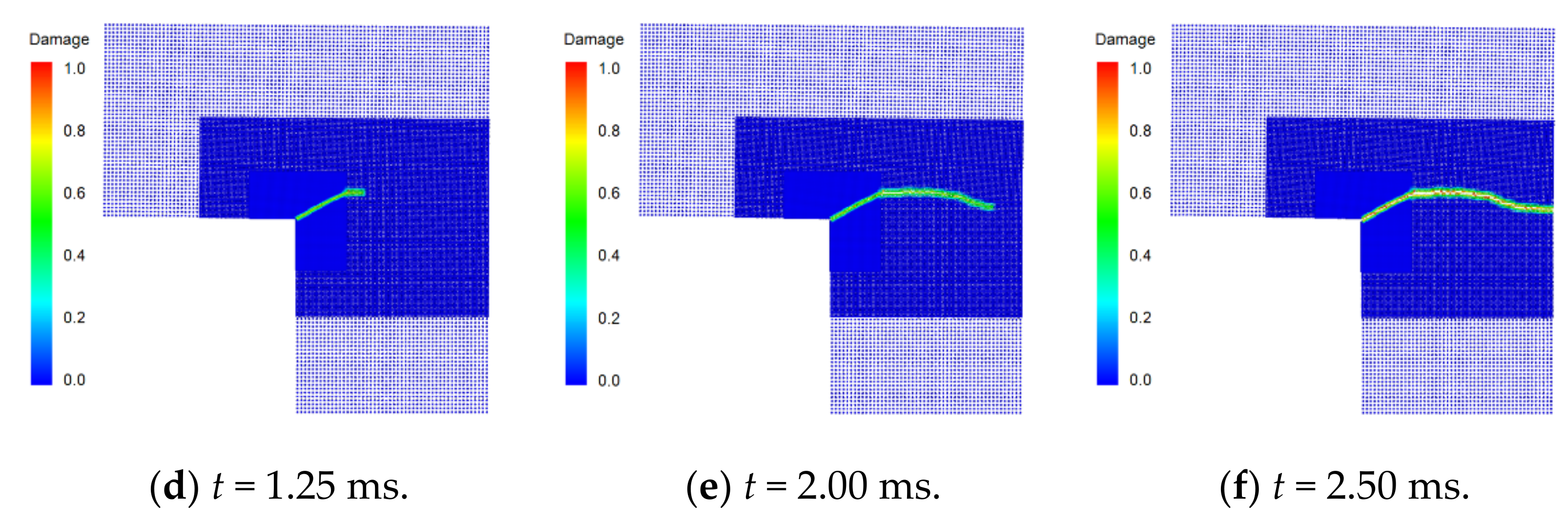
Figure 15 shows the simulated crack propagation in the L-shaped plate. At t = 0.65 ms, a crack appears at the corner point of the L-shaped plate and propagates in the direction of 26° on the horizontal. Then, the direction of crack propagation changes to horizontal at a time close to t = 1 ms. The transverse crack expands to the right boundary of the specimen and cuts across the plate when t = 2.5 ms.
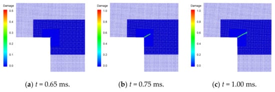
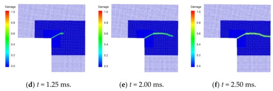
Figure 15.
Snapshots of simulated crack propagation in the L-shaped plate.
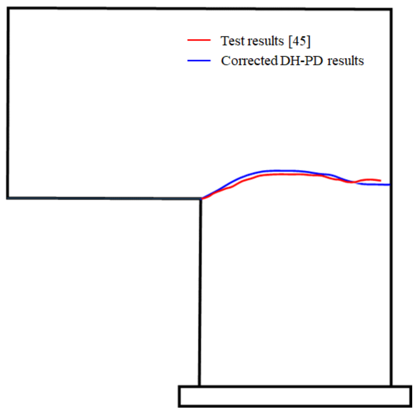
Figure 16 shows the numerical and experimental crack propagation paths. The simulated results essentially coincide with the experimental data recorded in the literature [45]. To quantitatively compare the results, the Pearson correlation coefficient of the experimental and numerical crack paths in Figure 16 is calculated. In this case, 52 points on the crack paths with an equal horizontal distance from the corner point are selected as the analysis objects. Assuming the vector X (x1, x2, x3, ……, x52) represents the calculated vertical coordinates of these points, and Y (y1, y2, y3, ……, y52) represents the measured ones in the experiment, the Pearson correlation coefficient of the two vectors can be calculated as:
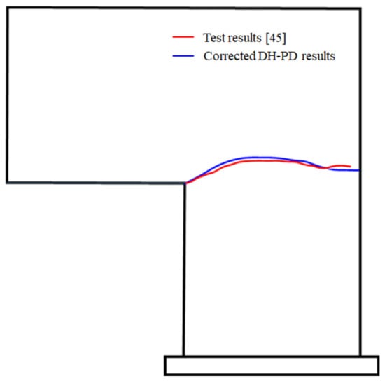
Figure 16.
Comparison of the numerical and experimental crack propagation paths [45].
In Equation (17), and are the average values of the two data sets, respectively.
According to Equation (17), the correlation coefficient between the experimental and numerical results is calculated to be 0.988, suggesting that the numerical results have a strong correlation with the experimental data. Therefore, the calculation accuracy of the presented DH-PD model is verified.
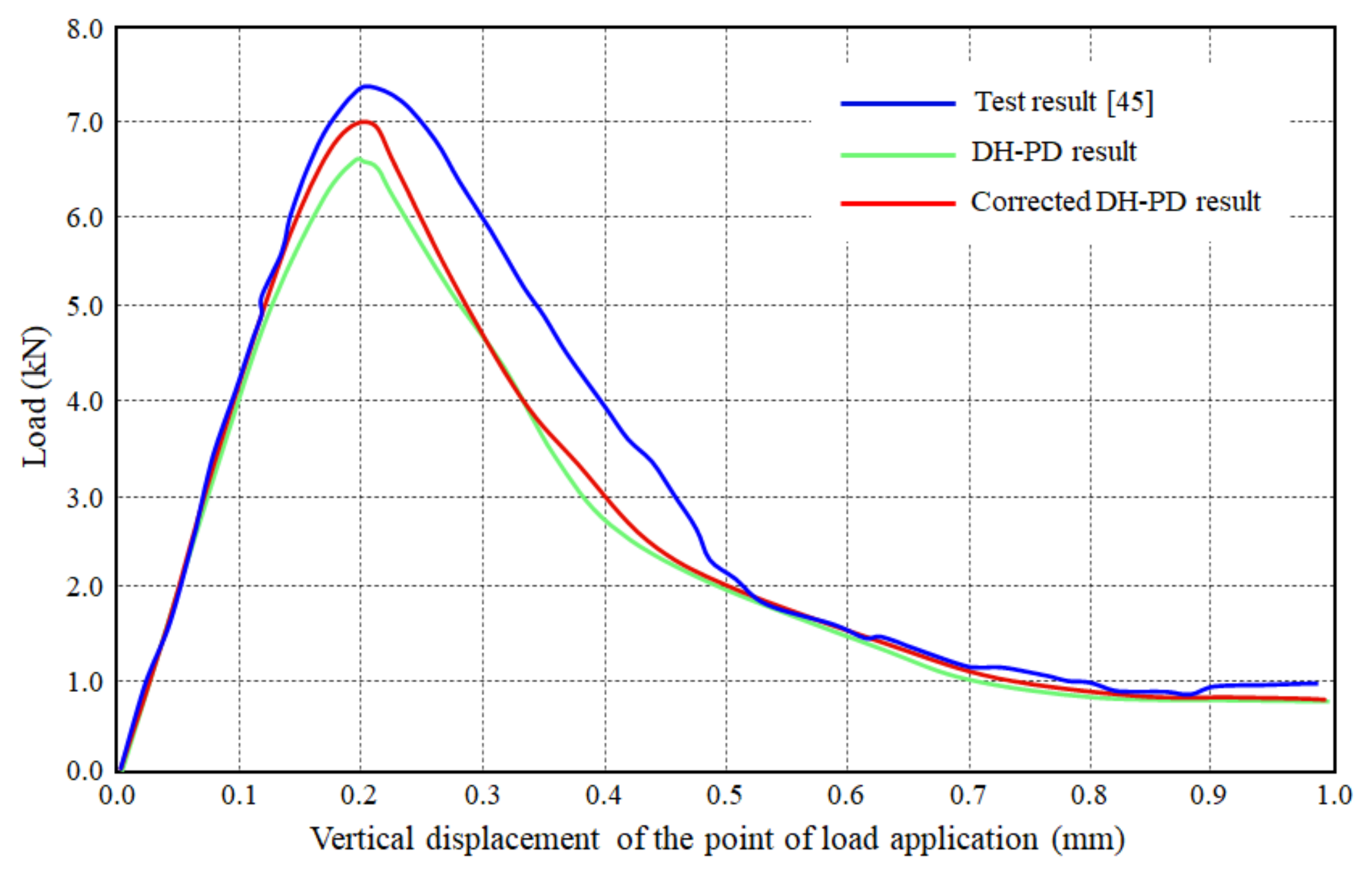
To quantitatively compare the numerical and experimental results, the load-displacement curves are obtained based on the numerical results, and are compared with the experimental data in Figure 17. The comparison shows that the varying tendencies of the simulated curves match the experimental data well, and the calculated peak values of the load are close to the test value, thus verifying the validity and applicability of the presented model. In addition, the figure also shows that the corrected DH-PD model has a relatively higher simulation accuracy than DH-PD model.
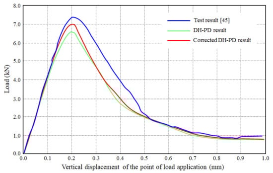
Figure 17.
Comparison of the numerical and experimental displacement–load curves [45].
4.4. Numerical Application 2: Mixed Damage of a DEN Specimen
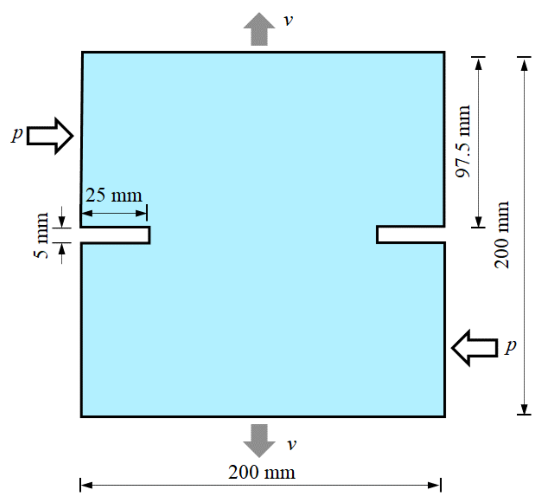
Figure 18 shows a square thin plate with a length of 200 mm on each side, an elastic modulus of E = 30 GPa, a density of ρ = 2265 kg/m3, a Poisson’s ratio of ν = 0.33, and energy release rates of GIc = 110 J/m2 and GIIc = 1100 J/m2. There is a prefabricated crack 25 mm in length and 5 mm in width on both sides of the specimen [46,47]. A uniform load, p, with a resultant force of 5 kN is applied in the horizontal direction on the left upper half and the right lower part of the plate. Meanwhile, a velocity load, v = 10 mm/s, is applied at the upper and lower boundaries of the plate, as shown in Figure 18.

Figure 18.
Geometric dimensions of a double-edged notched specimen.
The PD and DH-PD models are separately used to simulate this problem with the model parameters shown in Table 2. In the PD model, the square specimen is discretized into 25,440 particles with a spacing of Δx = Δy = 1.25 mm. In the DH-PD model, the specimen is discretized into two kinds of particles: 5280 finer particles with a spacing of Δx = Δy = 1.25 mm in the middle part of the specimen, and 5040 coarser particles with a spacing of Δx = Δy = 2.5 mm near the boundary of the specimen. The uniform force, p, on both sides is transformed into a physical load, p/Δy, which is applied to the particles at the outermost layer of the plate. The velocity load, v, is exerted on the three layers of particles at the upper and lower boundaries of the specimen. Finally, the step length is set to Δt = 0.1 μs.
Table 2.
Values of peridynamics parameters for the PD and DH-PD models.
Figure 19 shows the simulated crack propagation in the DEN specimen based on both the traditional PD model and the DH-PD model proposed in this work. The crack paths and the propagation velocities obtained from these two models match each other. To compare the computational efficiency of the two models, Table 3 shows the calculation times of the same simulation using both models. The DH-PD model drastically improves the use of computational resources largely by increasing efficiency by 119.4% under the same operation mode.
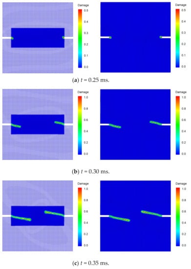
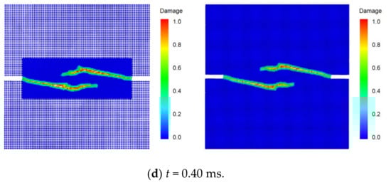
Figure 19.
Snapshots of simulated crack propagation in the double-edged notched specimen using the DH-PD model (left) and traditional PD model (right).
Table 3.
Calculation time and efficiency of the two models.
Figure 20 compares the simulated crack paths with experimental data obtained by Nooru-Mohamed et al. [47], those calculated by the FEM model proposed in [48], and the traditional PD model. All the simulated crack paths coincide with the experimental results. To quantitatively analyze the computational accuracy of the corrected DH-PD model, Table 4 lists the Pearson correlation coefficients of the numerical and experimental crack paths shown in Figure 20. The comparison demonstrates that the simulation results obtained by the corrected DH-PD model proposed in this study match the experimental results better than those obtained by other numerical models.
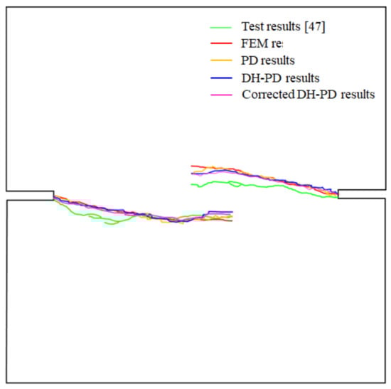
Figure 20.
Comparison of the experimental and numerical (from the models of current study and other numerical studies) crack paths [47,48].
Table 4.
Correlation coefficients between the test and numerical results on the crack paths.
5. Conclusions
In this study, an efficient DH-PD model was developed based on the PD theory and the concept of dual-horizon. In this model, a technique of nonuniformity discretization with variable horizons was incorporated, which significantly improved the computational efficiency. Moreover, volume correction and surface correction were introduced to improve computational accuracy of the model. Finally, the DH-PD model was verified and applied to simulate crack propagation problems, producing valuable results.
The presented DH-PD model was verified through the simulation of benchmark problems. After comparing the numerical results against the analytical solution and FDM results, high goodness of fit was obtained to verify the accuracy of the corrected DH-PD model. No spurious wave reflection was found during the simulation, confirming the advantage of the corrected DH-PD model over the traditional PD method. Additionally, the surface correction and particle volume correction could substantially reduce the calculation error.
In the simulation of the fracture of an L-shaped concrete specimen, the specimen was discretized into particles with three different sizes and varying horizons. The simulated crack propagation produced a crack path consistent with the experimental results. Based on the Pearson correlation coefficient for quantitatively comparing the results, the coefficient value of 0.988 verified the calculation accuracy of the presented DH-PD model.
The corrected DH-PD model simulates the mixed damage of a DEN specimen. The simulated crack paths were compared against the experimental data and the results obtained by the traditional PD model and the FEM model. The comparison showed that the corrected DP-PD model has a higher simulation accuracy than the FEM model and is computationally more efficient than the traditional PD method.
Author Contributions
Conceptualization, Z.D., L.W. and Z.L.; methodology, Z.D. and J.X.; writing—original draft preparation, Z.D. and J.X.; writing—review and editing, S.Q. and L.W.; visualization, J.X. and Z.L.; supervision, S.Q.; funding acquisition, Z.D., Z.L. and L.W. All authors have read and agreed to the published version of the manuscript.
Funding
This research was funded by the National Natural Science Foundation of China (Grant No. 42102318, 42002272, 41807266), the Program for Professor of Special Appointment (Eastern Scholar) at Shanghai Institutions of Higher Learning, and the Shanghai Science and Technology Innovation Action Plan (21DZ1204202).
Institutional Review Board Statement
Not applicable.
Informed Consent Statement
Not applicable.
Data Availability Statement
The data presented in this study are available on request from the corresponding author.
Acknowledgments
The authors are grateful for the support from the Department of Civil Engineering, Shanghai University.
Conflicts of Interest
The authors declare no conflict of interest.
References
- Ravi-Chandar, K. Dynamic Fracture of Nominally Brittle Materials. Int. J. Fract. 1998, 90, 83–102. [Google Scholar] [CrossRef]
- Ma, X.; Wang, F. The Fracture Analysis of Instop Gasket Using FEM Simulations. Adv. Sci. Lett. 2011, 4, 2573–2577. [Google Scholar] [CrossRef]
- Ramaswamy, K.; Babu, P.R. Fracture analysis of composite pressure vessel using FEM. Int. J. Comput. Mater. Sci. Eng. 2021, 10, 2150003. [Google Scholar] [CrossRef]
- Warren, T.L.; Silling, S.A.; Askari, A.; Weckner, O.; Epton, M.A.; Xu, J. A non-ordinary state-based peridynamic method to model solid material deformation and fracture. Int. J. Solids Struct. 2009, 46, 1186–1195. [Google Scholar] [CrossRef] [Green Version]
- Hou, C.-Y. Various remeshing arrangements for two-dimensional finite element crack closure analysis. Eng. Fract. Mech. 2017, 170, 59–76. [Google Scholar] [CrossRef]
- Bouchard, P.; Bay, F.; Chastel, Y.; Tovena, I. Crack propagation modelling using an advanced remeshing technique. Comput. Methods Appl. Mech. Eng. 2000, 189, 723–742. [Google Scholar] [CrossRef]
- Moës, N.; Dolbow, J.; Belytschko, T. A finite element method for crack growth without remeshing. Int. J. Numer. Methods Eng. 1999, 46, 131–150. [Google Scholar] [CrossRef]
- Chen, J.-W.; Zhou, X.-P. The enhanced extended finite element method for the propagation of complex branched cracks. Eng. Anal. Bound. Elem. 2019, 104, 46–62. [Google Scholar] [CrossRef]
- Unosson, M.; Olovsson, L.; Simonsson, K. Failure modelling in finite element analyses: Element erosion with crack-tip enhancement. Finite Elem. Anal. Des. 2006, 42, 283–297. [Google Scholar] [CrossRef]
- Alter, C.; Kolling, S.; Schneider, J. An enhanced non–local failure criterion for laminated glass under low velocity impact. Int. J. Impact Eng. 2017, 109, 342–353. [Google Scholar] [CrossRef]
- Wang, L.; Zhou, X. Phase field model for simulating the fracture behaviors of some disc-type specimens. Eng. Fract. Mech. 2020, 226, 106870. [Google Scholar] [CrossRef]
- Msekh, M.A.; Sargado, J.M.; Jamshidian, M.; Areias, P.M.; Rabczuk, T. Abaqus implementation of phase-field model for brittle fracture. Comput. Mater. Sci. 2015, 96, 472–484. [Google Scholar] [CrossRef]
- Zhu, Q.Z.; Ni, T.; Zhao, L.Y. Simulations of crack propagation in rock-like materials using peridynamic method. Chin. J. Rock Mech. Eng. 2016, 34, 3507–3515. (in Chinese). [Google Scholar]
- Cheng, Y.; Li, J. A complex variable meshless method for fracture problems. Sci. China Ser. G Phys. Mech. Astron. 2006, 49, 46–59. [Google Scholar] [CrossRef]
- Gao, H.; Cheng, Y. A Complex Variable Meshless Manifold Method for Fracture Problems. Int. J. Comput. Methods 2010, 7, 55–81. [Google Scholar] [CrossRef]
- Khazal, H.; Bayesteh, H.; Mohammadi, S.; Ghorashi, S.S.; Ahmed, A. An extended element free Galerkin method for fracture analysis of functionally graded materials. Mech. Adv. Mater. Struct. 2015, 23, 513–528. [Google Scholar] [CrossRef]
- Kou, M.M.; Han, D.C.; Xiao, C.C.; Wang, Y.T. Dynamic fracture instability in brittle materials: Insights from DEM simulations. Struct. Eng. Mech. 2019, 71, 65–75. [Google Scholar]
- Owayo, A.A.; Teng, F.C.; Chen, W.C. DEM simulation of crack evolution in cement-based materials under inclined shear test. Constr. Build. Mater. 2021, 301, 124087. [Google Scholar] [CrossRef]
- Silling, S. Reformulation of elasticity theory for discontinuities and long-range forces. J. Mech. Phys. Solids 2000, 48, 175–209. [Google Scholar] [CrossRef] [Green Version]
- Silling, S.; Askari, E. A meshfree method based on the peridynamic model of solid mechanics. Comput. Struct. 2005, 83, 1526–1535. [Google Scholar] [CrossRef]
- Oh, M.; Koo, B.; Kim, J.-H.; Cho, S. Shape design optimization of dynamic crack propagation using peridynamics. Eng. Fract. Mech. 2021, 252, 107837. [Google Scholar] [CrossRef]
- Ni, T.; Zaccariotto, M.; Zhu, Q.-Z.; Galvanetto, U. Static solution of crack propagation problems in Peridynamics. Comput. Methods Appl. Mech. Eng. 2019, 346, 126–151. [Google Scholar] [CrossRef]
- Hu, Y.; Madenci, E. Peridynamics for fatigue life and residual strength prediction of composite laminates. Compos. Struct. 2017, 160, 169–184. [Google Scholar] [CrossRef]
- Postek, E.; Sadowski, T. Impact model of the Al2O3/ZrO2 composite by peridynamics. Compos. Struct. 2021, 271, 114071. [Google Scholar] [CrossRef]
- Mikata, Y. Peridynamics for fluid mechanics and acoustics. Acta Mech. 2021, 232, 3011–3032. [Google Scholar] [CrossRef]
- Mikata, Y. Peridynamics for Heat Conduction. J. Heat Transf. 2020, 142, 081402. [Google Scholar] [CrossRef]
- Shou, Y.; Zhou, X. A coupled thermomechanical nonordinary state-based peridynamics for thermally induced cracking of rocks. Fatigue Fract. Eng. Mater. Struct. 2020, 43, 371–386. [Google Scholar] [CrossRef]
- Silling, S.A.; Lehoucq, R.B. Convergence of Peridynamics to Classical Elasticity Theory. J. Elast. 2008, 93, 13–37. [Google Scholar] [CrossRef]
- Liu, S.; Fang, G.; Liang, J.; Fu, M.; Wang, B. A new type of peridynamics: Element-based peridynamics. Comput. Methods Appl. Mech. Eng. 2020, 366, 113098. [Google Scholar] [CrossRef]
- Sun, W.; Fish, J. Coupling of non-ordinary state-based peridynamics and finite element method for fracture propagation in saturated porous media. Int. J. Numer. Anal. Methods Géoméch. 2021, 45, 1260–1281. [Google Scholar] [CrossRef]
- Ren, B.; Fan, H.; Bergel, G.L.; Regueiro, R.; Lai, X.; Li, S. A peridynamics–SPH coupling approach to simulate soil fragmentation induced by shock waves. Comput. Mech. 2015, 55, 287–302. [Google Scholar] [CrossRef]
- Zhang, Y.; Pan, G.; Zhang, Y.H.; Haeri, S. A multi-physics peridynamics-DEM-IB-CLBM framework for the prediction of erosive impact of solid particles in viscous fluids. Comput. Methods Appl. Mech. Eng. 2019, 352, 675–690. [Google Scholar] [CrossRef]
- DiPasquale, D.; Zaccariotto, M.; Galvanetto, U. Crack propagation with adaptive grid refinement in 2D peridynamics. Int. J. Fract. 2014, 190, 1–22. [Google Scholar] [CrossRef]
- Bobaru, F.; Yang, M.; Alves, L.F.; Silling, S.A.; Askari, E.; Xu, J. Convergence, adaptive refinement, and scaling in 1D peridynaics. Int. J. Numer. Methods Eng. 2009, 77, 852–877. [Google Scholar] [CrossRef] [Green Version]
- Shojaei, A.; Mossaiby, F.; Zaccariotto, M.; Galvanetto, U. An adaptive multi-grid peridynamic method for dynamic fracture analysis. Int. J. Mech. Sci. 2018, 144, 600–617. [Google Scholar] [CrossRef]
- Bazazzadeh, S.; Mossaiby, F.; Shojaei, A. An adaptive thermo-mechanical peridynamic model for fracture analysis in ceramics. Eng. Fract. Mech. 2020, 223, 106708. [Google Scholar] [CrossRef]
- Ren, H.; Zhuang, X.; Cai, Y.; Rabczuk, T. Dual-horizon peridynamics. Int. J. Numer. Methods Eng. 2016, 108, 1451–1476. [Google Scholar] [CrossRef] [Green Version]
- Rabczuk, T.; Ren, H. A peridynamics formulation for quasi-static fracture and contact in rock. Eng. Geol. 2017, 225, 42–48. [Google Scholar] [CrossRef]
- Wang, B.; Oterkus, S.; Oterkus, E. Derivation of dual-horizon state-based peridynamics formulation based on Euler–Lagrange equation. Contin. Mech. Thermodyn. 2020, 1–21. [Google Scholar] [CrossRef]
- Ren, H.; Zhuang, X.; Rabczuk, T. Dual-horizon peridynamics: A stable solution to varying horizons. Comput. Methods Appl. Mech. Eng. 2017, 318, 762–782. [Google Scholar] [CrossRef] [Green Version]
- Le, Q.V.; Bobaru, F. Surface corrections for peridynamic models in elasticity and fracture. Comput. Mech. 2018, 61, 499–518. [Google Scholar] [CrossRef]
- Scabbia, F.; Zaccariotto, M.; Galvanetto, U. A novel and effective way to impose boundary conditions and to mitigate the surface effect in state-based Peridynamics. Int. J. Numer. Methods Eng. 2021, 122, 5773–5811. [Google Scholar] [CrossRef]
- Madenci, E.; Oterkus, E. Peridynamic Theory and Its Applications. In Peridynamic Theory and Its Applications; Springer: Berlin/Heidelberg, Germany, 2014. [Google Scholar]
- Speronello, M. Study of Computational Peridynamics, Explicit and Implicit Time Integration, Viscoelastic Material; University of Padua: Padua, Italy, 2015. [Google Scholar]
- Winkler, B.; Hofstetter, G.; Niederwanger, G. Experimental verification of a constitutive model for concrete cracking. Proc. Inst. Mech. Eng. Part L J. Mater. Des. Appl. 2001, 215, 75–86. [Google Scholar] [CrossRef]
- Naderi, M.; Jung, J.; Yang, Q.D. A three dimensional augmented finite element for modeling arbitrary cracking in solids. Int. J. Fract. 2016, 197, 147–168. [Google Scholar] [CrossRef]
- Nooru-Mohamed, M.B.; Schlangen, E.; van Mier, J.G. Experimental and numerical study on the behavior of concrete subjected to biaxial tension and shear. Adv. Cem. Based Mater. 1993, 1, 22–37. [Google Scholar] [CrossRef]
- Ožbolt, J.; Reinhardt, H. Numerical study of mixed-mode fracture in concrete. Int. J. Fract. 2002, 118, 145–162. [Google Scholar] [CrossRef]


Publisher’s Note: MDPI stays neutral with regard to jurisdictional claims in published maps and institutional affiliations. |
© 2021 by the authors. Licensee MDPI, Basel, Switzerland. This article is an open access article distributed under the terms and conditions of the Creative Commons Attribution (CC BY) license (https://creativecommons.org/licenses/by/4.0/).