Mathematical Analysis of Biodegradation Model under Nonlocal Operator in Caputo Sense

Abstract

To lower the concentration of organic pollutants in the effluent stream, wastewater must be treated before being discharged into the environment. The question of whether wastewater treatment facilities can successfully reduce the concentration of micropollutants found in their influent streams is becoming increasingly pressing. The removal of micropollutants in treatment plants is investigated using a model that incorporates biodegradation and sorption as the key processes of micropollutant removal. This article provides the mathematical analysis of the wastewater model that describes the removal of micropollutant in treatment plants under a non-local operator in Caputo sense. The positivity of the solution is presented for the Caputo fractional model. The steady state’s solution of model and their stability is presented. The fixed point theorems of Leray–Schauder and Banach are used to deduce results regarding the existence of the solution of the model. Ulam–Hyers (UH) types of stabilities are presented via functional analysis. The fractional Euler method is used to find the numerical results of the proposed model. The numerical results are illustrated via graphs to show the effects of recycle ratio and the impact of fractional order on the evolution of the model.

1. Introduction and Motivation

Traditional wastewater treatment plants (WTP) are capable of removing bulk carbon-containing organic pollutants and also nutrients like nitrogen and phosphorus. They were not, however, constructed to eliminate organic pollutants identified in trace quantities, sometimes known as micropollutants [1]. Chemicals found in personal care items, such as active pharmaceutical ingredients and derivatives, as well as chemicals found in household goods, such as insecticides and surfactants, are examples of common micropollutants. Polycyclic aromatic hydrocarbons (PAHs), hormones, and metals, are examples of frequent micropollutants. Micropollutants have been proven to have an ecotoxic effect when released into aquatic environments. As a result, European legislation has been enacted that requires both businesses and governments to cut their emissions [2]. Pomies et al. [3] evaluated mathematical models for the removal of micropollutants in WTPs. In WTPs, micropollutants are eliminated via four major methods [3]. Biodegradation, cometabolism, mass transfer to the gas phase, and sorption onto particles are all examples of these processes. Not all pollutants are affected by these processes. By mass transfer into the gas phase, for instance, only volatile organic molecules are eliminated. For some pollutants, other processes may apply. Precipitation can, for example, eliminate heavy metals. One of the uses of mathematical models is determining the most important removal method for a specific pollutant. The activity of biomass in WTP can help eliminate micropollutants. This is also known as micropollutant bioconversion or biotransformation. Biodegradation and cometabolism are two mechanisms that might cause this change. In the context of the removal of micropollutants, there is no universally accepted definition of biodegradation [3]. The elimination of micropollutants via a mechanism unrelated to the microorganism’s development is a popular view. In addition, it is commonly thought that biodegradation occurs solely in the aqueous phase. Delgadillo-Mirquez et al. [4] have looked at this hypothesis. The term “cometabolism” refers to the breakdown of micropollutants in the presence of another quickly degradable substrate. Micropollutants are not a carbon source for microbial development in this scenario [5]. A metabolic process degrades a large number of organic micropollutants found in wastewater treatment plants. Many additional models [6,7,8,9] have been developed to explore WTPs in different ways. Nelson et al. presented a mathematical model in [10] that shows alternative techniques to removing micropollutants in the activated sludge process. They outline the biological events and processes that their model includes. Three biological reactions can be found. The activated sludge mechanism is linked to two of these, Equations (1) and (2). The degradation of micropollutants by biomass is the third process, shown in Equation (3). There are two physical processes in the model: The sorption of micropollutants onto suspended particles to generate particulate micropollutants as shown in Equation (4), and the desorption of particulates as shown in Equation (5). The biomass $\left({\mathbf{X}}_{\mathrm{B},\mathrm{H}}\right)$ consumes the soluble substrate ${\mathbf{S}}_s$ to create new biomass.

$${\mathbf{S}}_s\underset{{\mathbf{X}}_{\mathrm{B},\mathrm{H}}}{\overset{\mu \left({\mathbf{S}}_s\right)}{⟶}}{\mathbf{Y}}_{\mathrm{H}}{\mathcal{X}}_{\mathrm{B},\mathrm{H}},$$

(1)

where ${\mathbf{Y}}_{\mathrm{H}}$ denotes the coefficient of heterotrophic yield. The following reaction represents the death of particulate biomass:

$$\begin{array}{c}\hfill {\mathcal{X}}_{\mathrm{B},\mathrm{H}}\stackrel{{\mathrm{b}}_{\mathrm{H}}}{⟶}decayproducts,\end{array}$$

(2)

where ${\mathrm{b}}_{\mathrm{H}}$ denotes the coefficient of heterotrophic decay. Biological removal of micropollutants is given by:

$$\begin{array}{c}\hfill {\mathcal{C}}_s\underset{{\mathcal{X}}_{\mathrm{B},\mathrm{H}}}{\overset{{\mathrm{k}}_{bio}}{⟶}}products.\end{array}$$

(3)

Sorption is given by:

$$\begin{array}{c}\hfill {\mathcal{C}}_s+\mathrm{T}\mathrm{S}\mathrm{S}\stackrel{{\mathrm{k}}_{sor}}{⟶}{\mathcal{C}}_p,\end{array}$$

(4)

where ${\mathrm{k}}_{sor}$ denotes the kinetic constant for adsorption and $\mathrm{T}\mathrm{S}\mathrm{S}$ represents the total suspended solids. Desorption is given by:

$$\begin{array}{c}\hfill {\mathcal{C}}_p\stackrel{{\mathrm{k}}_{des}}{⟶}{\mathcal{C}}_s+\mathrm{T}\mathrm{S}\mathrm{S},\end{array}$$

(5)

where ${\mathrm{k}}_{des}$ denotes the kinetic constant for desorption. The Nelson model contains four contents explaining the activated sludge process and micropollutants. They formulated the dimensional model as:

$$\begin{array}{c}\hfill \left\{\begin{array}{c}\mathcal{V}\frac{d}{dt}{\mathcal{S}}_s=\mathfrak{F}({\mathcal{S}}_{s,in}-{\mathcal{S}}_s)-\frac{{\mu }_{max}}{{\mathbf{Y}}_{\mathrm{H}}}{\mathfrak{M}}_2\left({\mathcal{S}}_s\right){\mathcal{X}}_{\mathrm{B},\mathrm{H}}\mathcal{V},\hfill \\ \mathcal{V}\frac{d}{dt}{\mathcal{X}}_{\mathrm{B},\mathrm{H}}=\mathfrak{F}\left({\mathcal{X}}_{\mathrm{B},\mathrm{H},in}-{\mathcal{X}}_{\mathrm{B},\mathrm{H}}\right)+{\mu }_{max}{\mathfrak{M}}_2\left({\mathcal{S}}_s\right){\mathcal{X}}_{\mathrm{B},\mathrm{H}}\mathcal{V}+\mathfrak{R}\mathfrak{F}(\mathrm{C}-1){\mathcal{X}}_{\mathrm{B},\mathrm{H}}-{\mathrm{b}}_{\mathrm{H}}{\mathcal{X}}_{\mathrm{B},\mathrm{H}}\mathcal{V},\hfill \\ \mathcal{V}\frac{d}{dt}{\mathcal{C}}_s=\mathfrak{F}({\mathcal{C}}_{s,in}-{\mathcal{C}}_s)-\mathfrak{H}{\mathfrak{Q}}_{air}{\mathcal{C}}_s-\mathcal{V}{\mathrm{k}}_{sor}{\mathcal{X}}_{\mathrm{T}\mathrm{S}\mathrm{S}}{\mathcal{C}}_s+\mathcal{V}\frac{{\mathrm{k}}_{sor}}{{\mathrm{k}}_d}{\mathcal{C}}_p-\mathcal{V}{\mathfrak{R}}_{bio},\hfill \\ \mathcal{V}\frac{d}{dt}{\mathcal{C}}_p=\mathfrak{F}({\mathcal{C}}_{p,in}-{\mathcal{C}}_p)+\mathfrak{R}\mathfrak{F}(\mathrm{C}-1){\mathcal{C}}_p+\mathcal{V}{\mathrm{k}}_{sor}{\mathcal{X}}_{\mathrm{T}\mathrm{S}\mathrm{S}}{\mathcal{C}}_s-\mathcal{V}\frac{{\mathrm{k}}_{sor}}{{\mathrm{k}}_d}{\mathcal{C}}_p,\hfill \end{array}\right.\end{array}$$

(6)

where ${\mathfrak{M}}_2$ represents the monod growth kinetics. ${\mathfrak{M}}_2$ and residence time τ are, respectively, defined as:

$$\begin{array}{cc}\hfill {\mathfrak{M}}_2\left({\mathcal{S}}_s\right)& =\frac{{\mathcal{S}}_s}{{\mathrm{K}}_{\mathcal{S}}+\mathcal{S}},\hfill \\ \hfill \tau & =\frac{\mathcal{V}}{\mathfrak{F}}.\hfill \end{array}$$

The parameters ${\mathrm{k}}_d,{\mathfrak{R}}_{bio}$ and ${\mathcal{X}}_{\mathrm{T}\mathrm{S}\mathrm{S}}$ are, respectively, defined as:

$$\begin{array}{ccc}\hfill {\mathrm{k}}_d& =& \frac{{\mathrm{k}}_{sor}}{{\mathrm{k}}_{des}},\hfill \\ \hfill {\mathfrak{R}}_{bio}& =& {\mathrm{k}}_{bio}{\mathcal{X}}_{\mathrm{B},\mathrm{H}}{\mathcal{C}}_s,\hfill \\ \hfill {\mathcal{X}}_{\mathrm{T}\mathrm{S}\mathrm{S}}& =& {\mathrm{c}}_2{\mathcal{X}}_{\mathrm{B},\mathrm{H}},\hfill \end{array}$$

where ${\mathrm{c}}_2$ represents the conversion of chemical demand to total suspended solids.

Model (6) may now be converted to a dimensionless version by using the dimensionless variables as follows:

$${\mathcal{S}}^{*}=\frac{\mathcal{S}}{{\mathrm{K}}_{\mathcal{S}}},{\mathcal{X}}^{*}=\frac{{\mathcal{X}}_{\mathrm{B},\mathrm{H}}}{{\mathbf{Y}}_{\mathrm{H}}{\mathrm{K}}_{\mathcal{S}}},{\mathcal{C}}_s^{*}=\frac{{\mathcal{C}}_s}{{\mathcal{C}}_{s,in}},{\mathcal{C}}_p^{*}=\frac{{\mathcal{C}}_p}{{\mathcal{C}}_{s,in}}{t}^{*}={\mu }_{max}t.$$

The dimensionless model is described as follows:

$$\left\{\begin{array}{c}\frac{d}{d{t}^{*}}{\mathcal{S}}^{*}\left(t^{*}\right)=\frac{{\mathcal{S}}_{s,in}^{*}-{\mathcal{S}}^{*}}{{\tau }^{*}}-\frac{{\mathcal{S}}^{*}{\mathcal{X}}^{*}}{1+{\mathcal{S}}^{*}},\hfill \\ \frac{d}{d{t}^{*}}{\mathcal{X}}^{*}\left(t^{*}\right)=\frac{{\mathcal{X}}_0^{*}-{\mathcal{X}}^{*}}{{\tau }^{*}}+\frac{{\mathcal{S}}^{*}{\mathcal{X}}^{*}}{1+{\mathcal{S}}^{*}}-{\mathrm{b}}_{\mathrm{H}}^{*}{\mathcal{X}}^{*}+\frac{{\mathfrak{R}}^{*}{\mathcal{X}}^{*}}{{\tau }^{*}},\hfill \\ \frac{d}{d{t}^{*}}{\mathcal{C}}_s^{*}\left(t^{*}\right)=\frac{1-{\mathcal{C}}_s^{*}}{{\tau }^{*}}-{\mathfrak{Q}}_{\mathrm{e}}{\mathcal{C}}_{\mathrm{s}}^{*}-{\mathrm{k}}_{\mathrm{sor}}^{*}{\mathcal{C}}_{\mathrm{s}}^{*}{\mathcal{X}}^{*}+\frac{{\mathrm{k}}_{\mathrm{sor}}^{*}}{{\mathrm{k}}_{\mathrm{d}}^{*}}{\mathcal{C}}_{\mathrm{p}}^{*}-{\mathrm{k}}_{\mathrm{bio}}^{*}{\mathcal{X}}^{*}{\mathcal{C}}_{\mathrm{s}}^{*},\hfill \\ \frac{d}{d{t}^{*}}{\mathcal{C}}_p^{*}\left(t^{*}\right)=\frac{{\mathcal{C}}_{p,in}^{*}-{\mathcal{C}}_p^{*}}{{\tau }^{*}}+\frac{{\mathfrak{R}}^{*}{\mathcal{C}}_p^{*}}{{\tau }^{*}}+{\mathrm{k}}_{sor}^{*}{\mathcal{C}}_s^{*}{\mathcal{X}}^{*}-\frac{{\mathrm{k}}_{sor}^{*}}{{\mathrm{k}}_d^{*}}{\mathcal{C}}_p^{*},\hfill \end{array}\right.$$

(7)

where

$$\begin{array}{ccc}\hfill {\mathcal{C}}_{p,in}^{*}& =& \frac{{\mathcal{C}}_{p,in}}{{\mathcal{C}}_{s,in}},\hfill \\ \hfill {\mathcal{X}}_0^{*}& =& \frac{{\mathcal{X}}_0}{{\mathbf{Y}}_{\mathrm{H}}{\mathcal{S}}_s},\hfill \\ \hfill {\mathrm{k}}_d^{*}& =& {\mathrm{c}}_2{\mathrm{K}}_{\mathcal{S}}{\mathbf{Y}}_{\mathrm{H}}{\mathrm{k}}_d,\hfill \\ \hfill {\mathcal{S}}_{s,in}^{*}& =& \frac{{\mathcal{S}}_{s,in}}{{\mathrm{K}}_{\mathcal{S}}},\hfill \\ \hfill {\mathfrak{Q}}_e& =& \frac{\mathfrak{H}{\mathfrak{Q}}_{air}}{\mathcal{V}{\mu }_{max,\mathfrak{H}}},\hfill \\ \hfill {\mathfrak{R}}^{*}& =& \mathfrak{R}(\mathrm{C}-1),\hfill \\ \hfill {\mathrm{b}}_{\mathrm{H}}^{*}& =& \frac{{\mathrm{b}}_{\mathrm{H}}}{{\mu }_{max,\mathfrak{H}}},\hfill \\ \hfill {\mathrm{k}}_{bio}^{*}& =& \frac{{\mathrm{K}}_{\mathcal{S}}{\mathbf{Y}}_{\mathrm{H}}{\mathrm{k}}_{bio}}{{\mu }_{max,\mathfrak{H}}},\hfill \\ \hfill {\mathrm{k}}_{sor}^{*}& =& \frac{{\mathrm{c}}_2{\mathrm{K}}_{\mathcal{S}}{\mathbf{Y}}_{\mathrm{H}}{\mathrm{k}}_{sor}}{{\mu }_{max,\mathfrak{H}}},\hfill \\ \hfill {\tau }^{*}& =& \tau {\mu }_{max,\mathfrak{H}}.\hfill \end{array}$$

The initial values are ${\mathcal{S}}^{*}\left(0\right)={\mathcal{S}}_0^{*}>0,{\mathcal{X}}^{*}\left(0\right)={\mathcal{X}}_0^{*}\ge 0,$ ${\mathcal{C}}_s^{*}\left(0\right)={\mathcal{C}}_{s_0}^{*}\ge 0,$ and ${\mathcal{C}}_p^{*}\left(0\right)={\mathcal{C}}_{p_0}^{*}\ge 0.$

The description of all variables and parameters in model (6) and (7) are given below.

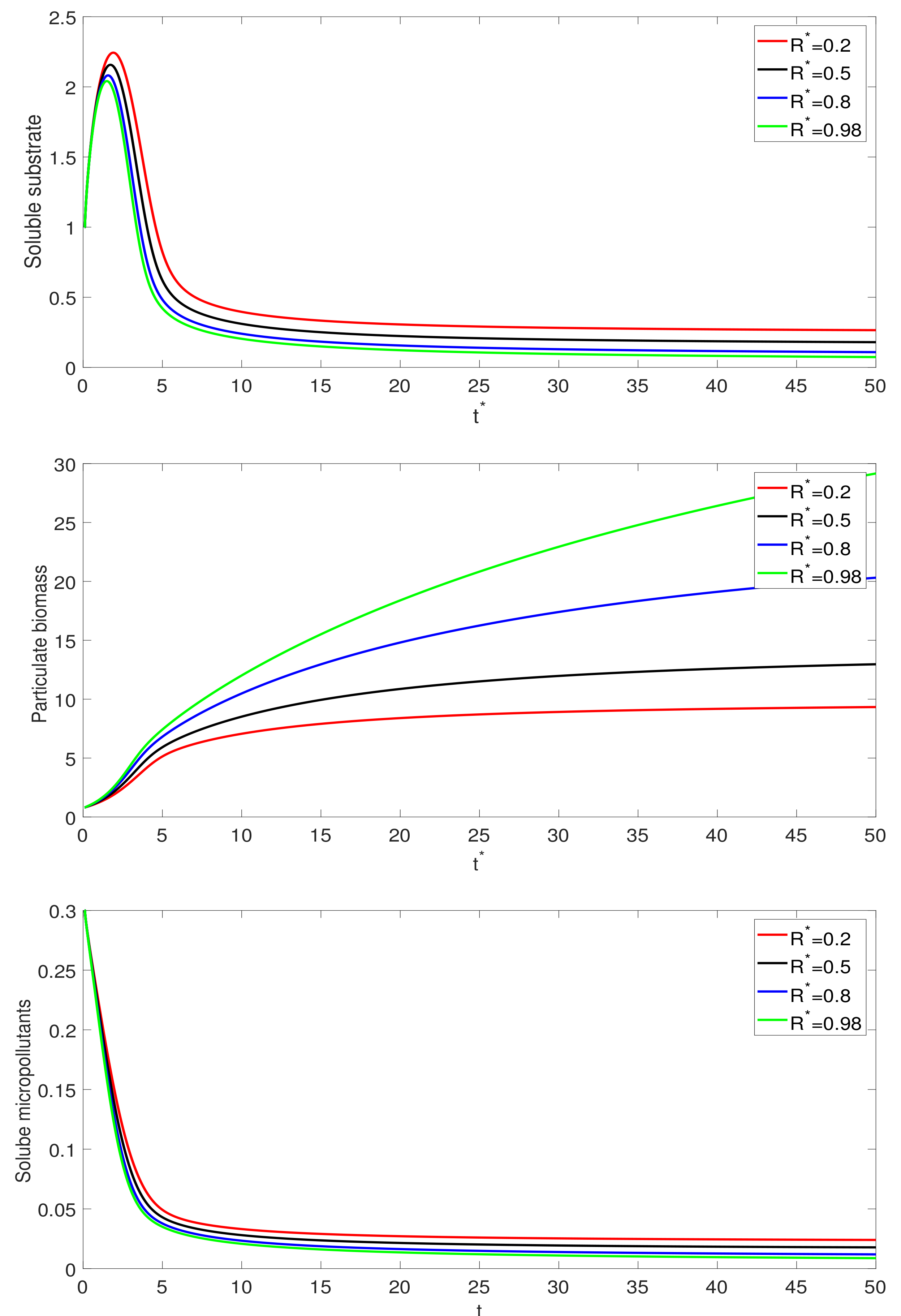
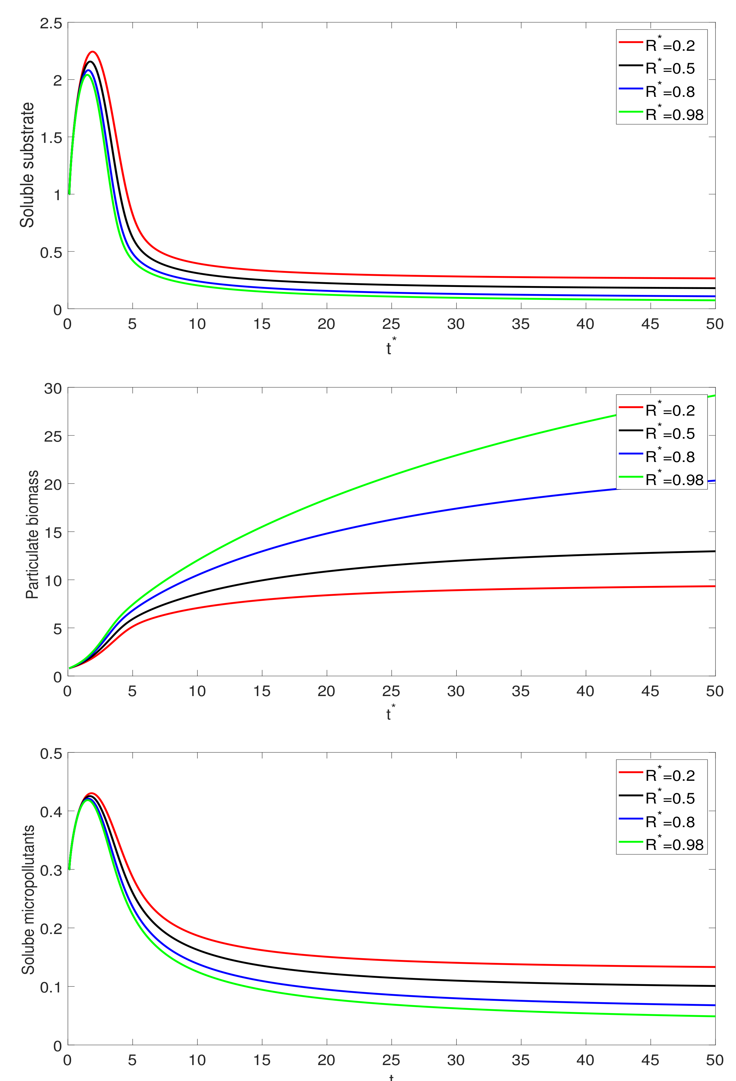
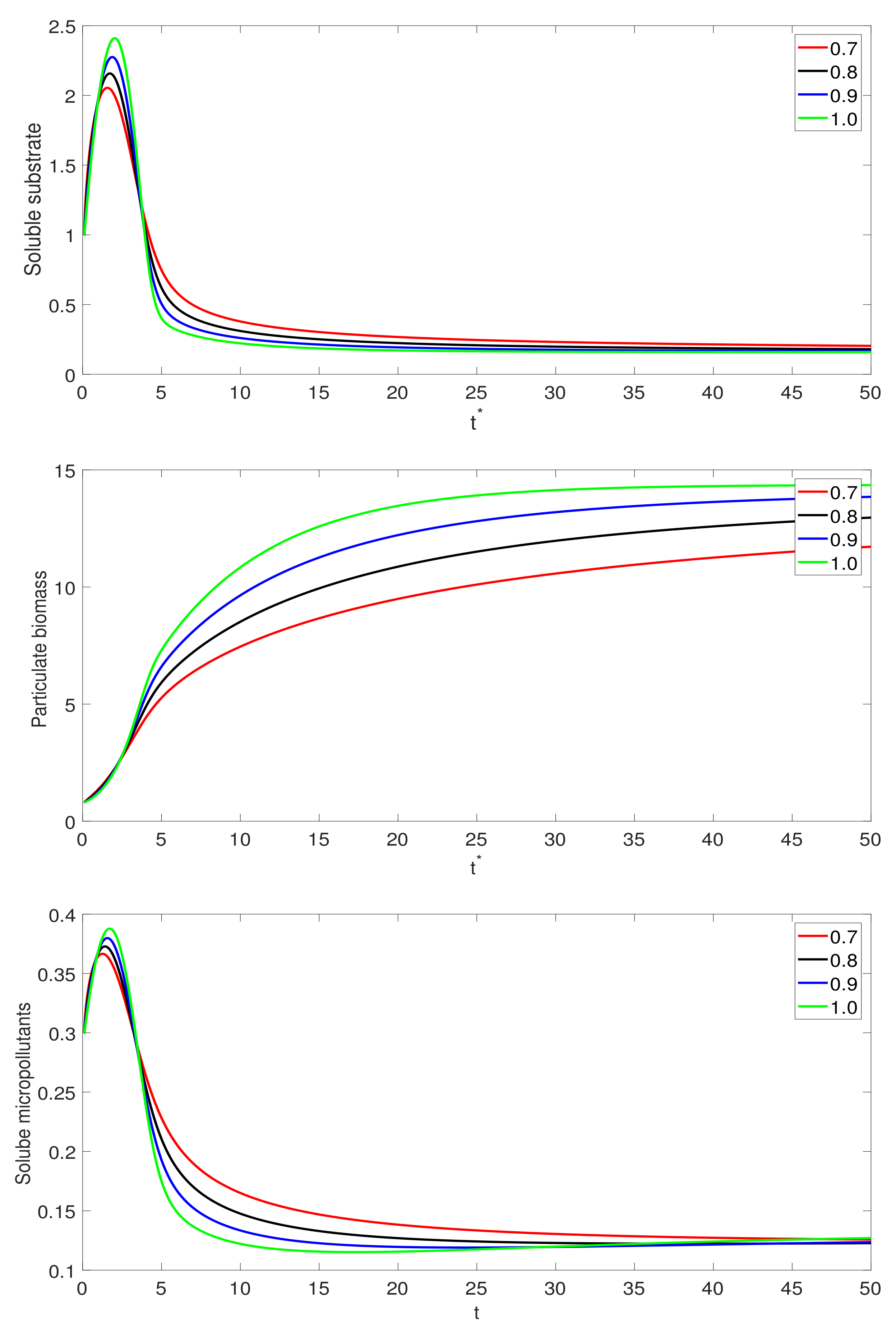
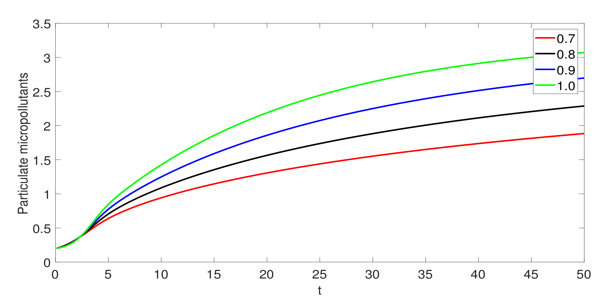
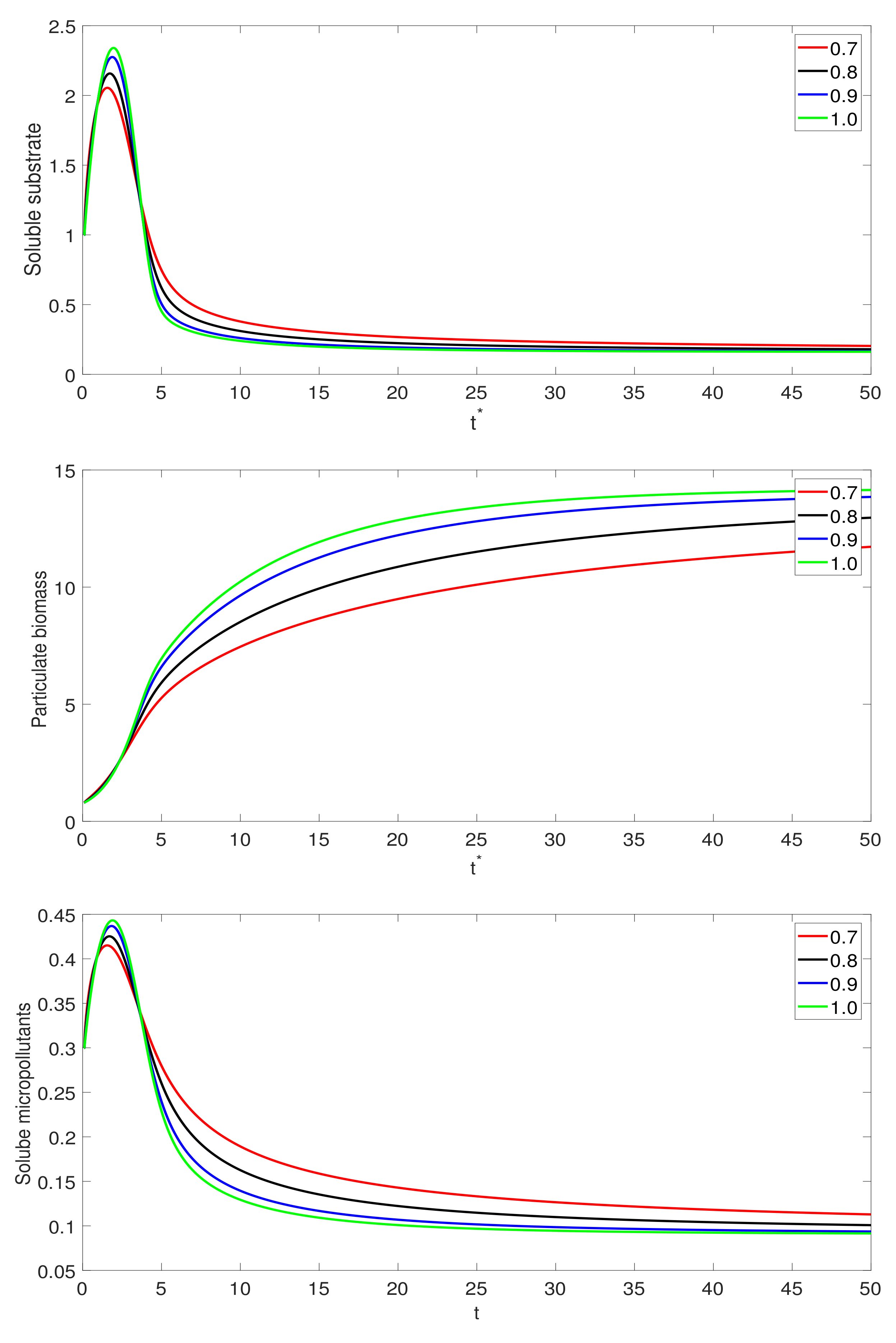
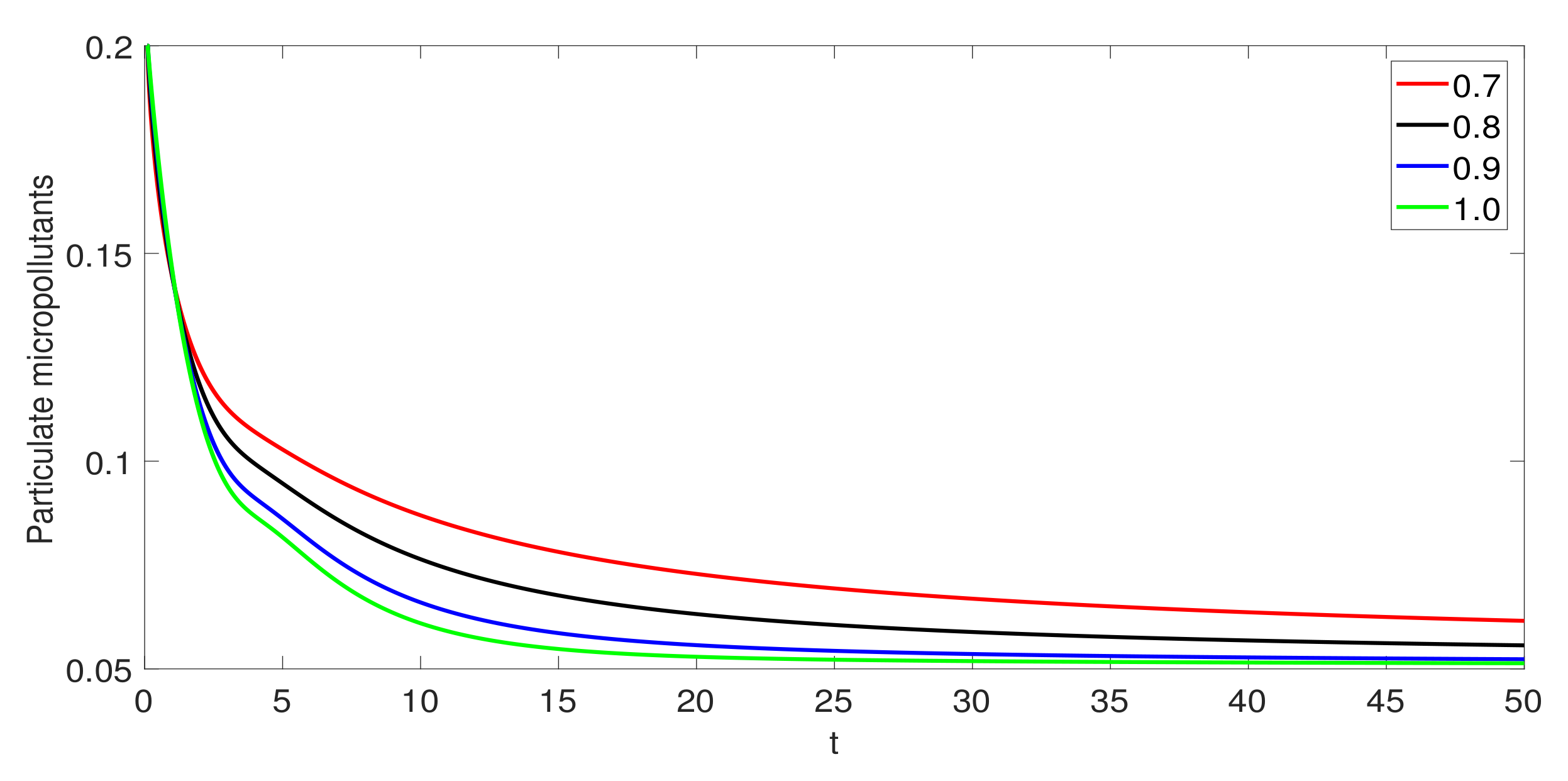
• ${\mathcal{S}}_s,{\mathcal{X}}_{\mathrm{B},\mathrm{H}},{\mathcal{C}}_s$ and ${\mathcal{C}}_p$ denote the soluble substrate, heterotroph (particulate biomass), soluble micropollutants, and particulate micropollutants, respectively.
• ${\mathcal{S}}_{s,in},\mathfrak{F},$ and $\mathcal{V}$ represent the substrate concentration in the feed, the flow rate through bioreactor, and the volume of the bioreactor, respectively.
• $\mathrm{C},{\mathcal{X}}_{\mathrm{B},\mathrm{H},in}$ and $\mathfrak{R}$ denote the recycle concentration factor, heterotroph concentration, and the recycle ratio, respectively.
• ${\mathrm{b}}_{\mathrm{H}},{\mathcal{C}}_{s,in},$ and ${\mathcal{X}}_{\mathrm{T}\mathrm{S}\mathrm{S}}$ denote the decay coefficient of particulate biomass, soluble micropollutants concentration, and the total suspended solids, respectively.
• ${\mathfrak{R}}_{bio},\tau$ represent the biological removal rate and residence time.
• $\mathfrak{H},{\mathfrak{Q}}_{air},$ and ${\mathcal{C}}_{p,in}$ represent the Henry coefficient of micropollutant, the flow rate of aeration, and the concentration of particulate micropollutants in the feed.

The memory and past history of a process can be determine by nonlocal operators in fractional calculus (FC). FC has lately been utilized to explain a wide range of difficult issues in the applied sciences [11,12]. Researchers have created mathematical theories to replicate the intricacies of nature using FC and to study memory and heredity features of a physical process. To construct mathematical models of real-world problems, differential operators (DOs) are used. DOs can be local or nonlocal (fractional). The three sorts of fractional operators that are most familiar are: The Caputo operator has a kernel with a power-law distribution [13]; a DO with exponential-decay law—called Caputo-Fabrizio operator [14]; and finally, an operator with Mittag–Leffler law—called the Atangana–Baleanu operator [15]. Researchers frequently use these operators to incorporate memory characteristics of theoretical models, which may be encountered in a wide range of disciplines of study [16,17,18].

Researchers have investigated the fractional differential equations from different points of view. Boundary value problems for Hilfer fractional differential inclusions with nonlocal integral boundary conditions have been studied by Wongcharoen et al. in [19]. Existence and Ulam–Hyers–Mittag–Leffler stability results of $\mathsf{\Psi }$ Hilfer nonlocal Cauchy problem is given in [20]. Hyers–Ulam stability and existence of solutions to the generalized Liouville–Caputo fractional differential equations have been investigated in [21]. Ahmed et al. investigated the solutions for the impulsive fractional pantograph differential equation via generalized anti-periodic boundary conditions in [22]. The numerical solution of fractional-order ordinary differential equations using the reformulated infinite state representation was proposed by Hinze and his coauthors [23]. Beside this, FC also has applications in biochemical models. Recently, Alqahtani et al. investigated the fractional order bioethanol production model [24]. Qureshi et al. used the fractional operator to study the blood ethanol model in [25]. In the literature [26], the authors analyzed the WWTPS model via fractional order. Some applications of fractional operators in a biochemical model are included in [27,28]. Inspired from the above studies, we study model (7) under a nonlocal operator in Caputo sense. We write model (7) in a Caputo operator as:

$$\left\{\begin{array}{c}{\mathcal{D}}_{t^{*}}^{\delta }{\mathcal{S}}^{*}\left(t^{*}\right)=\frac{{\mathcal{S}}_{s,in}^{*}-{\mathcal{S}}^{*}}{{\tau }^{*}}-\frac{{\mathcal{S}}^{*}{\mathcal{X}}^{*}}{1+{\mathcal{S}}^{*}},\hfill \\ {\mathcal{D}}_{t^{*}}^{\delta }{\mathcal{X}}^{*}\left(t^{*}\right)=\frac{{\mathcal{X}}_0^{*}-{\mathcal{X}}^{*}}{{\tau }^{*}}+\frac{{\mathcal{S}}^{*}{\mathcal{X}}^{*}}{1+{\mathcal{S}}^{*}}-{\mathrm{b}}_{\mathrm{H}}^{*}{\mathcal{X}}^{*}+\frac{{\mathfrak{R}}^{*}{\mathcal{X}}^{*}}{{\tau }^{*}},\hfill \\ {\mathcal{D}}_{t^{*}}^{\delta }{\mathcal{C}}_s^{*}\left(t^{*}\right)=\frac{1-{\mathcal{C}}_s^{*}}{{\tau }^{*}}-{\mathfrak{Q}}_{\mathrm{e}}{\mathcal{C}}_{\mathrm{s}}^{*}-{\mathrm{k}}_{\mathrm{sor}}^{*}{\mathcal{C}}_{\mathrm{s}}^{*}{\mathcal{X}}^{*}+\frac{{\mathrm{k}}_{\mathrm{sor}}^{*}}{{\mathrm{k}}_{\mathrm{d}}^{*}}{\mathcal{C}}_{\mathrm{p}}^{*}-{\mathrm{k}}_{\mathrm{bio}}^{*}{\mathcal{X}}^{*}{\mathcal{C}}_{\mathrm{s}}^{*},\hfill \\ {\mathcal{D}}_{t^{*}}^{\delta }{\mathcal{C}}_p^{*}\left(t^{*}\right)=\frac{{\mathcal{C}}_{p,in}^{*}-{\mathcal{C}}_p^{*}}{{\tau }^{*}}+\frac{{\mathfrak{R}}^{*}{\mathcal{C}}_p^{*}}{{\tau }^{*}}+{\mathrm{k}}_{sor}^{*}{\mathcal{C}}_s^{*}{\mathcal{X}}^{*}-\frac{{\mathrm{k}}_{sor}^{*}}{{\mathrm{k}}_d^{*}}{\mathcal{C}}_p^{*},\hfill \end{array}\right.$$

(8)

subject to the initial conditions ${\mathcal{S}}^{*}\left(0\right)={\mathcal{S}}_0^{*}>0,{\mathcal{X}}^{*}\left(0\right)={\mathcal{X}}_0^{*}\ge 0,$ ${\mathcal{C}}_s^{*}\left(0\right)={\mathcal{C}}_{s_0}^{*}\ge 0,$ and ${\mathcal{C}}_p^{*}\left(0\right)={\mathcal{C}}_{p_0}^{*}\ge 0.$

The fractional operator was not used to study model (7) in the literature. As a result, we examine the biodegradation model using the Caputo derivative. The aforementioned model’s theoretical and computational features are investigated. Using well-known fixed point theorems like Banach’s and Larey-nonlinear Schauder’s alternative, the main purpose of this research is to investigate the existence and uniqueness of the model’s solutions. The stability study is also looked at from several types of Ulam stabilities. Finally, we use the fractional Euler technique to get the approximate solutions to the biodegradation model’s fractional model. The numerical results are graphically presented to study the evolution of the proposed model against different fractional orders.

Now we provide some basic notions of fractional calculus, which are needed in the paper. FD and FI represent the fractional derivative and fractional integral, respectively.

Definition 1

([13]). For a continuous function $\mathcal{H}$ on $[0,T]$, the FD in the case of Caputo is defined as:

$${\mathcal{D}}_t^{\delta }\mathcal{H}\left(t\right)=\frac{1}{\Gamma (j-\delta )}\left[{\int }_0^t{(t-\kappa )}^{j-\delta -1}\frac{d^j}{d{\kappa }^j}\mathcal{H}\left(t\right)\left(\kappa \right)d\kappa \right],$$

for the integers part $\left[\delta \right]$ of δ, $j=\left[\delta \right]+1$.

Definition 2

([13]). Let $\mathcal{H}\in L^1([0,T],\mathbb{R})$, an FI in Riemann–Liouvilli sense of order $0<\delta \le 1$ is defined as:

$$I^{\delta }\mathcal{H}\left(t\right)=\frac{1}{\Gamma \left(\delta \right)}{\int }_0^t{(t-\kappa )}^{\delta -1}\mathcal{H}\left(\kappa \right)d\kappa .$$

Definition 3

(Banach contraction result). Let $Ø\ne \mathbb{B}\subset \mathcal{A}$ be a closed subset of a Banach space $\mathcal{A}$. If the operator $\mathfrak{U}:\mathbb{B}\to \mathbb{B}$ satisfies the contraction condition, then $\mathfrak{U}$ has a unique fixed point.

Definition 4

(Leray–Schauder fixed point theorem). Consider a closed and convex subset ${\mathbb{B}}_r^{*}$ of $\mathcal{A}$ and an open subset $\mathbb{P}$ of $\mathcal{A}$, also $0\in \mathbb{P}$. If $\mathfrak{U}:\overline{\mathbb{P}}\to$${\mathbb{B}}_r^{*}$ is a continuous and compact function. Then either $\mathfrak{U}$ possesses a fixed point in $\overline{\mathbb{P}}$ or $\exists \mathcal{Y}\in \partial$$\overline{\mathbb{P}}$ and $\psi \in (0,1)$ such that $\mathcal{Y}=\psi \mathfrak{U}\left(\mathcal{Y}\right)$.

2. Mathematical Analysis

In this section, we look at some of the model’s key features, such as non-negative solutions, the existence of a unique solution for the suggested model, and several forms of Ulam’s stability results. Using fractional Euler’s technique, we establish the numerical solutions for the investigated model.

2.1. Theoretical Analysis

In this section, we examine the theoretical aspects of the proposed model.

Lemma 1

(Non-negativity of the solution). If the initial conditions are non-negative then the solutions of (8) are non-negative, for all $t>0$.

Proof. 

As all of the parameters and initial conditions are positive. So from the proposed model we get

$${\mathcal{D}}_{t^{*}}^{\delta }{\mathcal{S}}^{*}\left(t^{*}\right){\mid }_{{\mathcal{S}}^{*}=0}=\frac{{\mathcal{S}}_{s,in}^{*}}{{\tau }^{*}}\ge 0,$$

$${\mathcal{D}}_{t^{*}}^{\delta }{\mathcal{X}}^{*}\left(t^{*}\right){\mid }_{{\mathcal{X}}^{*}=0}=\frac{{\mathcal{X}}_0^{*}}{{\tau }^{*}}\ge 0,$$

$${\mathcal{D}}_{t^{*}}^{\delta }{\mathcal{C}}_s^{*}\left(t^{*}\right){\mid }_{{\mathcal{C}}_s^{*}=0}=\frac{1}{{\tau }^{*}}+\frac{{\mathrm{k}}_{\mathrm{sor}}^{*}}{{\mathrm{k}}_{\mathrm{d}}^{*}}{\mathcal{C}}_{\mathrm{p}}^{*}\ge 0,$$

$${\mathcal{D}}_{t^{*}}^{\delta }{\mathcal{C}}_p^{*}\left(t^{*}\right){\mid }_{{\mathcal{C}}_p^{*}=0}=\frac{{\mathcal{C}}_{p,in}^{*}}{{\tau }^{*}}+{\mathrm{k}}_{sor}^{*}{\mathcal{C}}_s^{*}{\mathcal{X}}^{*}\ge 0.$$

As a consequence, the suggested model’s solutions are all non-negative.  □

2.1.1. Steady States and Its Stability

• The proposed model has two steady states. The first one is the washout branch (${\mathrm{W}}_0$), when ${\mathcal{X}}^{*}=0$. The washout branch is given by

  $${\mathrm{W}}_0=\left({\mathcal{S}}_{s,in}^{*},0,1,0\right).$$
  The second one is the no-washout branch (${\mathrm{W}}^{*}$), when ${\mathcal{X}}^{*}>0.$ The no-washout branch is given by:

  $${\mathrm{W}}^{*}=\left({\mathcal{S}}_1^{*},\frac{{\mathcal{S}}_{s,in}^{*}-{\mathcal{S}}_1^{*}}{1-{\mathfrak{R}}^{*}+{\mathrm{b}}_{\mathrm{H}}^{*}{\tau }^{*}},f_1\left[1-{\mathfrak{R}}^{*}+{\tau }^{*}\frac{{\mathrm{k}}_{sor}^{*}}{{\mathrm{k}}_d^{*}}\right],f_1{\tau }^{*}{\mathrm{k}}_{sor}^{*}{\mathcal{X}}^{*}\right),$$

  where

  $$\begin{array}{ccc}\hfill {\mathcal{S}}_1^{*}& =& \frac{1-{\mathfrak{R}}^{*}+{\mathrm{b}}_{\mathrm{H}}^{*}{\tau }^{*}}{(1-{\mathrm{b}}_{\mathrm{H}}^{*}){\tau }^{*}-(1-{\mathfrak{R}}^{*})},\hfill \\ \hfill f_1& =& \frac{1}{\left[\left(\frac{{\mathrm{k}}_{sor}^{*}}{{\mathrm{k}}_d^{*}}\right)f_2+{\mathrm{k}}_{sor}^{*}{\mathcal{X}}^{*}(1-{\mathfrak{R}}^{*})\right]{\tau }^{*}+f_2(1-{\mathfrak{R}}^{*})},\hfill \\ \hfill f_2& =& 1+{\mathrm{k}}_{bio}^{*}{\mathcal{X}}^{*}{\tau }^{*}.\hfill \end{array}$$
  Now, we present the local stability (LS) of the steady states. Consider the Jacobian matrix as:

  $$\mathsf{J}=\left[\begin{array}{cccc}-\frac{1}{{\tau }^{*}}-\frac{{\mathcal{X}}^{*}}{{\left(1+{\mathcal{S}}^{*}\right)}^2}& -\frac{{\mathcal{S}}^{*}}{1+{\mathcal{S}}^{*}}& 0& 0\\ \frac{{\mathcal{X}}^{*}}{{\left(1+{\mathcal{S}}^{*}\right)}^2}& \frac{{\mathfrak{R}}^{*}-1-{\mathrm{b}}_{\mathrm{H}}^{*}{\tau }^{*}}{{\tau }^{*}}+\frac{{\mathcal{S}}^{*}}{1+{\mathcal{S}}^{*}}& 0& 0\\ 0& -({\mathrm{k}}_{sor}^{*}+{\mathrm{k}}_{bio}^{*}){\mathcal{C}}_s^{*}& -\frac{1}{{\tau }^{*}}-{\mathcal{X}}^{*}({\mathrm{k}}_{sor}^{*}+{\mathrm{k}}_{bio}^{*})& \frac{{\mathrm{k}}_{sor}^{*}}{{\mathrm{k}}_d^{*}}\\ 0& {\mathrm{k}}_{sor}^{*}{\mathcal{C}}_s^{*}& {\mathrm{k}}_{sor}^{*}{\mathcal{X}}^{*}& -\frac{1-{\mathfrak{R}}^{*}}{{\tau }^{*}}-\frac{{\mathrm{k}}_{sor}^{*}}{{\mathrm{k}}_d^{*}}\end{array}\right].$$
• For the LS of the washout solution branch, consider the eigenvalues of $\mathsf{J}$ at the washout branch as:

  $$\begin{array}{ccc}\hfill {\Lambda }_{1,2}& =& -\frac{1}{{\tau }^{*}}<0,\hfill \\ \hfill {\Lambda }_3& =& \frac{{\mathfrak{R}}^{*}-1-\frac{{\mathrm{k}}_{sor}^{*}}{{\mathrm{k}}_d^{*}}{\tau }^{*}}{{\tau }^{*}}<0,\hfill \\ \hfill {\Lambda }_4& =& \frac{{\mathfrak{R}}^{*}-1-{\mathrm{b}}_{\mathrm{H}}^{*}{\tau }^{*}}{{\tau }^{*}}+\frac{{\mathcal{S}}_{s,in}^{*}}{1+{\mathcal{S}}_{s,in}^{*}}.\hfill \end{array}$$
  Since ${\mathfrak{R}}^{*}\in [0,1).$ The eigenvalue ${\Lambda }_4<0$ when

  $$\left[{\mathcal{S}}_{s,in}^{*}-{\mathrm{b}}_{\mathrm{H}}^{*}({\mathcal{S}}_0^{*}+1)\right]{\tau }^{*}<({\mathcal{S}}_{s,in}^{*}+1)(1-{\mathfrak{R}}^{*}).$$
  It follows that ${\Lambda }_4<0$ when

  $${\mathrm{b}}_{\mathrm{H}}^{*}\ge \frac{{\mathcal{S}}_{s,in}^{*}}{1+{\mathcal{S}}_{s,in}^{*}}.$$
  Otherwise, for ${\mathrm{b}}_{\mathrm{H}}^{*}<\frac{{\mathcal{S}}_{s,in}^{*}}{1+{\mathcal{S}}_{s,in}^{*}}$, the WSS is LS if ${\tau }^{*}$ is enough low:

  $${\tau }^{*}<{\tau }_{cr}^{*}=\frac{\left({\mathcal{S}}_{s,in}^{*}+1\right)(1-{\mathfrak{R}}^{*})}{{\mathcal{S}}_{s,in}^{*}-{\mathrm{b}}_{\mathrm{H}}^{*}({\mathcal{S}}_{s,in}^{*}+1)}.$$
• For an LS of no-washout solution branch, from the second equation of model (8), we have

  $${\mathcal{X}}^{*}\left(\frac{{\mathfrak{R}}^{*}-1}{{\tau }^{*}}+\frac{{\mathcal{S}}^{*}}{1+{\mathcal{S}}^{*}}-{\mathrm{b}}_{\mathrm{H}}^{*}\right)=0.$$
  For the no-washout branch ${\mathcal{X}}^{*}\ne 0,$ so

  $$\left(\frac{{\mathfrak{R}}^{*}-1}{{\tau }^{*}}+\frac{{\mathcal{S}}^{*}-{\mathrm{b}}_{\mathrm{H}}^{*}({\mathcal{S}}^{*}+1)}{{\mathcal{S}}^{*}+1}\right)=0.$$
  For the above equation, the characteristic polynomail of $\mathsf{J}$ is as follows:

  $$\mathrm{G}(\Lambda )={\left({\Lambda }^2+a\Lambda +b\right)}^2\left({\Lambda }^2+a_1\Lambda +a_2{a}_3\right),$$

  (9)

  where

  $$\begin{array}{cc}\hfill a& =\frac{1}{{\tau }^{*}}+{\mathcal{X}}^{*}({\mathrm{k}}_{bio}^{*}+{\mathrm{k}}_{sor}^{*})+\frac{1-{\mathfrak{R}}^{*}}{{\tau }^{*}}+\frac{{\mathrm{k}}_{sor}^{*}}{{\mathrm{k}}_d^{*}},\hfill \\ \hfill b& =\left(\frac{1}{{\tau }^{*}}+{\mathcal{X}}^{*}({\mathrm{k}}_{sor}^{*}+{\mathrm{k}}_{bio}^{*})\right)\left(\frac{1-{\mathfrak{R}}^{*}}{{\tau }^{*}}+\frac{{\mathrm{k}}_{sor}^{*}}{{\mathrm{k}}_d^{*}}\right)-\frac{{\mathrm{k}}_{sor}^{{*}^2}}{{\mathrm{k}}_d^{*}}{\mathcal{X}}^{*},\hfill \\ \hfill a_1& =\frac{1}{{\tau }^{*}}+\frac{{\mathcal{X}}^{*}}{{\left(1+{\mathcal{S}}^{*}\right)}^2},\hfill \\ \hfill a_2& =\frac{{\mathcal{S}}^{*}}{1+{\mathcal{S}}^{*}},\hfill \\ \hfill a_3& =\frac{{\mathcal{X}}^{*}}{{\left(1+{\mathcal{S}}^{*}\right)}^2}.\hfill \end{array}$$
  The no-washout solution is of interest when all solution are positive. So, in these cases, the coefficients of $\mathsf{J}$ are positive. From the above equations, we see that $a>0$, $a_3>0$, $a_1>0$ and $a_2{a}_3>0.$ To prove that $b>0,$ consider

  $$\begin{array}{cc}\hfill b& =\left(\frac{1}{{\tau }^{*}}+{\mathcal{X}}^{*}({\mathrm{k}}_{sor}^{*}+{\mathrm{k}}_{bio}^{*})\right)\left(\frac{1-{\mathfrak{R}}^{*}}{{\tau }^{*}}+\frac{{\mathrm{k}}_{sor}^{*}}{{\mathrm{k}}_d^{*}}\right)-\frac{{\mathrm{k}}_{sor}^{{*}^2}}{{\mathrm{k}}_d^{*}}{\mathcal{X}}^{*}\hfill \\ \hfill & =\frac{\left(\frac{1-{\mathfrak{R}}^{*}}{{\tau }^{*}}+\frac{{\mathrm{k}}_{sor}^{*}}{{\mathrm{k}}_d^{*}}\right)+{\mathcal{X}}^{*}{\tau }^{*}\frac{{\mathrm{k}}_{sor}^{*}}{{\mathrm{k}}_d^{*}}{\mathrm{k}}_{bio}^{*}+{\mathcal{X}}^{*}({\mathrm{k}}_{sor}^{*}+{\mathrm{k}}_{bio}^{*})(1-{\mathfrak{R}}^{*})}{{\tau }^{*}}>0.\hfill \end{array}$$
  Thus $b>0,$ so no-washout solution branch is LS.

2.1.2. Applications of Fixed Point Theory to the Existence of Solution

We establish that there is at least one unique solution to the given model using the Leray–Schauder theorem and the Banach fixed point theorems in this section. Let us write the model’s right-hand side (8) as follows:

$$\left\{\begin{array}{c}{\mathbb{G}}_1(t^{*},{\mathcal{S}}^{*})=\frac{{\mathcal{S}}_{s,in}^{*}-{\mathcal{S}}^{*}}{{\tau }^{*}}-\frac{{\mathcal{S}}^{*}{\mathcal{X}}^{*}}{1+{\mathcal{S}}^{*}},\hfill \\ {\mathbb{G}}_2(t^{*},{\mathcal{X}}^{*})=\frac{{\mathcal{X}}_0^{*}-{\mathcal{X}}^{*}}{{\tau }^{*}}+\frac{{\mathcal{S}}^{*}{\mathcal{X}}^{*}}{1+{\mathcal{S}}^{*}}-{\mathrm{b}}_{\mathrm{H}}^{*}{\mathcal{X}}^{*}+\frac{{\mathfrak{R}}^{*}{\mathcal{X}}^{*}}{{\tau }^{*}},\hfill \\ {\mathbb{G}}_3(t^{*},{\mathcal{C}}_s^{*})=\frac{1-{\mathcal{C}}_s^{*}}{{\tau }^{*}}-{\mathfrak{Q}}_{\mathrm{e}}{\mathcal{C}}_{\mathrm{s}}^{*}-{\mathrm{k}}_{\mathrm{sor}}^{*}{\mathcal{C}}_{\mathrm{s}}^{*}{\mathcal{X}}^{*}+\frac{{\mathrm{k}}_{\mathrm{sor}}^{*}}{{\mathrm{k}}_{\mathrm{d}}^{*}}{\mathcal{C}}_{\mathrm{p}}^{*}-{\mathrm{k}}_{\mathrm{bio}}^{*}{\mathcal{X}}^{*}{\mathcal{C}}_{\mathrm{s}}^{*},\hfill \\ {\mathbb{G}}_4(t^{*},{\mathcal{C}}_p^{*})=\frac{{\mathcal{C}}_{p,in}^{*}-{\mathcal{C}}_p^{*}}{{\tau }^{*}}+\frac{{\mathfrak{R}}^{*}{\mathcal{C}}_p^{*}}{{\tau }^{*}}+{\mathrm{k}}_{sor}^{*}{\mathcal{C}}_s^{*}{\mathcal{X}}^{*}-\frac{{\mathrm{k}}_{sor}^{*}}{{\mathrm{k}}_d^{*}}{\mathcal{C}}_p^{*}.\hfill \end{array}\right.$$

(10)

Model (8) becomes:

$$\left\{\begin{array}{c}{\mathcal{D}}_{t^{*}}^{\delta }{\mathcal{S}}^{*}\left(t^{*}\right)={\mathbb{G}}_1(t^{*},{\mathcal{S}}^{*}),\hfill \\ {\mathcal{D}}_{t^{*}}^{\delta }{\mathcal{X}}^{*}\left(t^{*}\right)={\mathbb{G}}_2(t^{*},{\mathcal{X}}^{*}),\hfill \\ {\mathcal{D}}_{t^{*}}^{\delta }{\mathcal{C}}_s^{*}\left(t^{*}\right)={\mathbb{G}}_3(t^{*},{\mathcal{C}}_s^{*}),\hfill \\ {\mathcal{D}}_{t^{*}}^{\delta }{\mathcal{C}}_p^{*}\left(t^{*}\right)={\mathbb{G}}_4(t^{*},{\mathcal{C}}_p^{*}).\hfill \end{array}\right.$$

(11)

Application of FI gives:

$$\left\{\begin{array}{c}{\mathcal{S}}^{*}\left(t^{*}\right)={\mathcal{S}}^{*}\left(0\right)+\frac{1}{\Gamma \left(\delta \right)}{\int }_0^{t^{*}}{\left(t^{*}-\kappa \right)}^{\delta -1}{\mathbb{G}}_1(\kappa ,{\mathcal{S}}^{*})d\kappa ,\hfill \\ {\mathcal{X}}^{*}\left(t^{*}\right)={\mathcal{X}}^{*}\left(0\right)+\frac{1}{\Gamma \left(\delta \right)}{\int }_0^{t^{*}}{\left(t^{*}-\kappa \right)}^{\delta -1}{\mathbb{G}}_2(\kappa ,{\mathcal{X}}^{*})d\kappa ,\hfill \\ {\mathcal{C}}_s^{*}\left(t^{*}\right)={\mathcal{C}}_s^{*}\left(0\right)+\frac{1}{\Gamma \left(\delta \right)}{\int }_0^{t^{*}}{\left(t^{*}-\kappa \right)}^{\delta -1}{\mathbb{G}}_3(\kappa ,{\mathcal{C}}_s^{*})d\kappa ,\hfill \\ {\mathcal{C}}_p^{*}\left(t^{*}\right)={\mathcal{C}}_p^{*}\left(0\right)+\frac{1}{\Gamma \left(\delta \right)}{\int }_0^{t^{*}}{\left(t^{*}-\kappa \right)}^{\delta -1}{\mathbb{G}}_4(\kappa ,{\mathcal{C}}_p^{*})d\kappa .\hfill \end{array}\right.$$

(12)

Let

$$\begin{array}{ccc}\hfill \mathcal{Y}\left(t^{*}\right)& =& \left(\begin{array}{c}{\mathcal{S}}^{*}\left(t^{*}\right)\\ {\mathcal{X}}^{*}\left(t^{*}\right)\\ {\mathcal{C}}_s^{*}\left(t^{*}\right)\\ {\mathcal{C}}_p^{*}\left(t^{*}\right)\end{array}\right),\hfill \\ \hfill \mathcal{Z}(t^{*},\mathcal{Y}\left(t^{*}\right))& =& \left(\begin{array}{c}{\mathbb{G}}_1(t^{*},{\mathcal{S}}^{*})\\ {\mathbb{G}}_2(t^{*},{\mathcal{X}}^{*})\\ {\mathbb{G}}_3(t^{*},{\mathcal{C}}_s^{*})\\ {\mathbb{G}}_3(t^{*},{\mathcal{C}}_p^{*})\end{array}\right),\hfill \end{array}$$

$$\begin{array}{ccc}\hfill {\mathcal{Y}}_0& =& \left(\begin{array}{c}{\mathcal{S}}_0^{*}\\ {\mathcal{X}}_0^{*}\\ {\mathcal{C}}_{s_0}^{*}\\ {\mathcal{C}}_{p_0}^{*}\end{array}\right).\hfill \end{array}$$

Equation (12) gets the form:

$$\mathcal{Y}\left(t^{*}\right)={\mathcal{Y}}_0+\frac{1}{\Gamma \left(\delta \right)}{\int }_0^{t^{*}}{\left(t^{*}-\kappa \right)}^{\delta -1}\mathcal{Z}(\kappa ,\mathcal{Y}\left(\kappa \right))d\kappa .$$

(13)

Let $\mathcal{A}=\mathfrak{C}\left([0,\mathrm{T}],{\mathbb{R}}^4\right)$ denotes a Banach space associated with a norm:

$$∥\mathcal{Y}∥=∥{\mathcal{S}}^{*},{\mathcal{X}}^{*},{\mathcal{C}}_s^{*},{\mathcal{C}}_p^{*}∥=\underset{t^{*}\in [0,\mathrm{T}]}{sup}\left|\mathcal{Y}\left(t^{*}\right)\right|,$$

(14)

where $\left|\mathcal{Y}\left(t^{*}\right)\right|=\left|{\mathcal{S}}^{*}\left(t^{*}\right)+{\mathcal{X}}^{*}\left(t^{*}\right)+{\mathcal{C}}_s^{*}\left(t^{*}\right)+{\mathcal{C}}_p^{*}\left(t^{*}\right)\right|,$ where ${\mathcal{S}}^{*},{\mathcal{X}}^{*},{\mathcal{C}}_s^{*},{\mathcal{C}}_p^{*}\in \mathcal{A}.$ If (13) admits a fixed point then it must have a solution. Let us define an operator $\mathfrak{U}:\mathcal{A}\to \mathcal{A}$. In the view of (13), we define $\mathfrak{U}$ as:

$$\left(\mathfrak{U}\mathcal{Y}\right)\left(t^{*}\right)={\mathcal{Y}}_0+\frac{1}{\Gamma \left(\delta \right)}{\int }_0^{t^{*}}{\left(t^{*}-\kappa \right)}^{\delta -1}\mathcal{Z}(\kappa ,\mathcal{Y}\left(\kappa \right))d\kappa .$$

(15)

Converting the examined model to a fixed point problem to establish fixed point theory, i.e., $\mathcal{Y}=\mathfrak{U}\mathcal{Y}.$ The following definition guarantees that the model has at least one solution.

Definition 5

(Existence of solution). Assume that:

$\left(C_1\right)$ For all $t^{*}\in [0,\mathrm{T}]$ and $\mathcal{Y}\in \mathcal{A}$ ∃ ${\alpha }_{\mathcal{Z}}>0$ and ${\beta }_{\mathcal{Z}}>0$ such that:

$$\left|\mathcal{Z}(t^{*},\mathcal{Y}\left(t^{*}\right))\right|\le {\alpha }_{\mathcal{Z}}\left|\mathcal{Y}\right|+{\beta }_{\mathcal{Z}}.$$

(16)

$\left(C_2\right)$ If $\exists \zeta >0$ such that:

$$\frac{\zeta }{∥{\mathcal{Y}}_0∥+\frac{({\alpha }_{\mathcal{Z}}r+{\beta }_{\mathcal{Z}}){\mathrm{T}}^{\delta }}{\Gamma (\delta +1)}}<1,$$

(17)

and $\mathcal{Z}$ is a continuous function. Then, Equation (13) has at least one solution.

Proof. 

Consider the operator which is defined by (15). First, we prove that $\mathfrak{U}$ maps bounded balls into bounded balls in $\mathcal{A}.$ Consider a bounded ball as: ${\mathbb{B}}_r^{*}=\left\{\mathcal{Y}\in \mathcal{A}:∥\mathcal{Y}∥\le r\right\},$ where $r>0.$ From Equation (13), we have

$$\begin{array}{ccc}\hfill \underset{t^{*}\in [0,\mathrm{T}]}{sup}\left|\left(\mathfrak{U}\mathcal{Y}\right)\left(t^{*}\right)\right|& =& ∥{\mathcal{Y}}_0+\frac{1}{\Gamma \left(\delta \right)}{\int }_0^{t^{*}}{\left(t^{*}-\kappa \right)}^{\delta -1}\mathcal{Z}(\kappa ,\mathcal{Y}\left(\kappa \right))d\kappa ∥\hfill \\ & \le & ∥{\mathcal{Y}}_0∥+∥\frac{1}{\Gamma \left(\delta \right)}{\int }_0^{t^{*}}{\left(t^{*}-\kappa \right)}^{\delta -1}\mathcal{Z}(\kappa ,\mathcal{Y}\left(\kappa \right))d\kappa ∥\hfill \\ & \le & ∥{\mathcal{Y}}_0∥+\frac{1}{\Gamma \left(\delta \right)}{\int }_0^{t^{*}}{\left(t^{*}-\kappa \right)}^{\delta -1}∥\mathcal{Z}(s,\mathcal{Y}(s\left)\right)∥d\kappa \hfill \\ & \le & ∥{\mathcal{Y}}_0∥+\underset{t^{*}\in [0,\mathrm{T}]}{sup}\frac{1}{\Gamma \left(\delta \right)}{\int }_0^{t^{*}}{\left(t^{*}-\kappa \right)}^{\delta -1}\left|\mathcal{Z}(s,\mathcal{Y}(s\left)\right)\right|d\kappa .\hfill \end{array}$$

Using mathematics and assumption $\left(C_1\right)$, we get

$$\begin{array}{ccc}\hfill ∥\mathfrak{U}\mathcal{Y}∥& \le & ∥{\mathcal{Y}}_0∥+\frac{{\mathrm{T}}^{\delta }}{\Gamma (\delta +1)}\left({\alpha }_{\mathcal{Z}}∥\mathcal{Y}∥+{\beta }_{\mathcal{Z}}\right)\le r.\hfill \end{array}$$

Thus, $\mathfrak{U}\left({\mathbb{B}}_r^{*}\right)\subset {\mathbb{B}}_r^{*}.$ Now, it is shown that $\mathfrak{U}$ maps bounded balls into equi-continuous sets of $\mathcal{A}.$ For $\mathcal{Y}\in {\mathbb{B}}_r^{*}$ and $z_1,z_2\in [0,\mathrm{T}]$ with $z_1<z_2$, we have

$$\begin{array}{ccc}\hfill \left|\left(\mathfrak{U}\mathcal{Y}\right)\left(z_2\right)-\left(\mathfrak{U}\mathcal{Y}\right)\left(z_1\right)\right|& =& \left|{\mathcal{Y}}_0+\frac{1}{\Gamma \left(\delta \right)}{\int }_0^{z_2}{\left(z_2-\kappa \right)}^{\delta -1}\mathcal{Z}(\kappa ,\mathcal{Y}\left(\kappa \right))d\kappa \right.\hfill \\ & & \left.-{\mathcal{Y}}_0-\frac{1}{\Gamma \left(\delta \right)}{\int }_0^{z_1}{\left(z_1-\kappa \right)}^{\delta -1}\mathcal{Z}(\kappa ,\mathcal{Y}\left(\kappa \right))d\kappa \right|\hfill \\ & \le & \frac{1}{\Gamma \left(\delta \right)}{\int }_0^{z_2}{\left(z_2-\kappa \right)}^{\delta -1}\left|\mathcal{Z}(\kappa ,\mathcal{Y}(\kappa \left)\right)\right|d\kappa \hfill \\ & & -\frac{1}{\Gamma \left(\delta \right)}{\int }_0^{z_1}{\left(z_1-\kappa \right)}^{\delta -1}\left|\mathcal{Z}(\kappa ,\mathcal{Y}(\kappa \left)\right)\right|d\kappa \hfill \\ & \le & \frac{{\alpha }_{\mathcal{Z}}r+{\beta }_{\mathcal{Z}}}{\Gamma (\delta +1)}\left(z_2^{\delta }-z_1^{\delta }\right).\hfill \end{array}$$

Clearly, $\left|\left(\mathfrak{U}\mathcal{Y}\right)\left(z_2\right)-\left(\mathfrak{U}\mathcal{Y}\right)\left(z_1\right)\right|\to 0$ as $z_2\to z_1.$ Thanks to the Arzela–Ascoli theorem, $\mathfrak{U}:\mathcal{A}\to \mathcal{A}$ is completely continuous. Finally, we show that all solutions to $\mathcal{Y}=\psi \mathfrak{U}\mathcal{Y},$ where $\psi \in (0,1),$ are bounded. Then, for $t^{*}\in [0,\mathrm{T}],$ one gets

$$\begin{array}{ccc}\hfill \left|\mathcal{Y}\left(t^{*}\right)\right|& =& \left|\psi \left(\mathfrak{U}\mathcal{Y}\right)\left(t^{*}\right)\right|\hfill \\ & \le & \left|\left(\mathfrak{U}\mathcal{Y}\right)\left(t^{*}\right)\right|\hfill \\ & \le & \left|{\mathcal{Y}}_0+\frac{1}{\Gamma \left(\delta \right)}{\int }_0^{t^{*}}{\left(t^{*}-\kappa \right)}^{\delta -1}\mathcal{Z}(\kappa ,\mathcal{Y}\left(\kappa \right))d\kappa \right|\hfill \\ & \le & \left|{\mathcal{Y}}_0\right|+\frac{\left({\alpha }_{\mathcal{Z}}r+{\beta }_{\mathcal{Z}}\right)t^{{*}^{\delta }}}{\Gamma (\delta +1)}.\hfill \end{array}$$

After some manipulation and taking the maximum value of $t^{*}\in [0,\mathrm{T}],$ one has

$$\frac{\mathcal{Y}}{∥{\mathcal{Y}}_0∥+\frac{({\alpha }_{\mathcal{Z}}r+{\beta }_{\mathcal{Z}}){\mathrm{T}}^{\delta }}{\Gamma (\delta +1)}}\le 1.$$

(18)

From assumption ($C_2$), $\exists \zeta >0$ such that $∥\mathcal{Y}∥\ne \zeta .$ Now, let $\mathbb{P}=\left\{\mathcal{Y}\in \mathcal{A}:∥\mathcal{Y}∥<\zeta \right\}.$ Note that $\mathfrak{U}:\overline{\mathbb{P}}\to {\mathbb{B}}_r^{*}$ is completely continuous. From $\overline{\mathbb{P}}$, ∄$\mathcal{Y}\in \partial \mathbb{P}$ with $\mathcal{Y}=\psi \mathfrak{U}\mathcal{Y},$ for some $\psi \in (0,1).$ Hence, by the fixed point theorem of Leray–Schauder, $\mathfrak{U}$ possesses a fixed point $\mathcal{Y}\in \overline{\mathbb{P}}$. As an outcome, the considered model must have at least one solution.  □

Definition 6

(Unique solution). Assume that:

$\left(A_3\right)$ For any ${\mathcal{Y}}_1$,${\mathcal{Y}}_2\in \mathcal{A}$ and $\forall t^{*}\in [0,\mathrm{T}]$, ∃ ${\hslash }_{\mathcal{Z}}>0$ such that

$$\left|\mathcal{Z}(t^{*},{\mathcal{Y}}_1\left(t^{*}\right))-\mathcal{Z}(t^{*},{\mathcal{Y}}_2\left(t^{*}\right))\right|\le {\hslash }_{\mathcal{Z}}\left|{\mathcal{Y}}_1\left(t^{*}\right)-{\mathcal{Y}}_2\left(t^{*}\right)\right|.$$

(19)

If $\frac{{\hslash }_{\mathcal{Z}}{\mathrm{T}}^{\zeta }}{\Gamma (\zeta +1)}<1,$ then the proposed model has a unique solution.

Proof. 

We use the contraction theorem of Banach, to prove that the model under discussion has a unique solution. Let ${\mathbb{B}}_r^{*}=\left\{\mathcal{Y}\in \mathcal{A}:∥\mathcal{Y}∥\le r\right\}$. As proved above, $\mathfrak{U}{\mathbb{B}}_r^{*}\subset {\mathbb{B}}_r^{*}.$ Lastly, we show that $\mathfrak{U}:{\mathbb{B}}_r^{*}\to {\mathbb{B}}_r^{*}$ is a contraction. For any ${\mathcal{Y}}_1,{\mathcal{Y}}_2\in \mathcal{A},$ one gets

$$\begin{array}{ccc}\hfill \underset{t^{*}\in [0,\mathrm{T}]}{sup}\left|\left(\mathfrak{U}{\mathcal{Y}}_1\right)\left(t^{*}\right)-\left(\mathfrak{U}{\mathcal{Y}}_2\right)\left(t^{*}\right)\right|& =& ∥{\mathcal{Y}}_0+\frac{1}{\Gamma \left(\delta \right)}{\int }_0^{t^{*}}{\left(t^{*}-\kappa \right)}^{\delta -1}\mathcal{Z}(\kappa ,{\mathcal{Y}}_1\left(\kappa \right))d\kappa \hfill \\ & & -{\mathcal{Y}}_0-\frac{1}{\Gamma \left(\delta \right)}{\int }_0^{t^{*}}{\left(t^{*}-\kappa \right)}^{\delta -1}\mathcal{Z}(\kappa ,{\mathcal{Y}}_2\left(\kappa \right))d\kappa ∥\hfill \\ & \le & ∥\frac{1}{\Gamma \left(\delta \right)}{\int }_0^{t^{*}}{\left(t^{*}-\kappa \right)}^{\delta -1}\left[\mathcal{Z}(\kappa ,{\mathcal{Y}}_1\left(\kappa \right))-\mathcal{Z}(\kappa ,{\mathcal{Y}}_2\left(\kappa \right))\right]d\kappa ∥\hfill \\ & \le & \frac{1}{\Gamma \left(\delta \right)}{\int }_0^{t^{*}}{\left(t^{*}-\kappa \right)}^{\delta -1}∥\left[\mathcal{Z}(\kappa ,{\mathcal{Y}}_1\left(\kappa \right))-\mathcal{Z}(\kappa ,{\mathcal{Y}}_2\left(\kappa \right))\right]∥d\kappa \hfill \\ & \le & \frac{{\hslash }_{\mathcal{Z}}}{\Gamma \left(\delta \right)}{\int }_0^{t^{*}}{\left(t^{*}-\kappa \right)}^{\delta -1}∥{\mathcal{Y}}_1-{\mathcal{Y}}_2∥d\kappa \hfill \\ & \le & \frac{{\hslash }_{\mathcal{Z}}{\mathrm{T}}^{\zeta }}{\Gamma (\zeta +1)}∥{\mathcal{Y}}_1-{\mathcal{Y}}_2∥.\hfill \end{array}$$

Since $\frac{{\hslash }_{\mathcal{Z}}{\mathrm{T}}^{\zeta }}{\Gamma (\zeta +1)}<1$, it means that $\mathfrak{U}$ is a contraction. By the Banach contraction theorem, $\mathfrak{U}$ possesses a unique fixed point. As a result, there is at most one solution to the problem under consideration.  □

2.1.3. Ulam–Hyers Stability

We will explore the theory for several forms of Ulam–Hyers (UH) stability in this part. We begin by defining several Ulam stabilizers for the model under discussion. Let $\sigma >0$ and a continuous mapping ${\mathcal{L}}_{\mathcal{Z}}:[0,\mathrm{T}]\times {\mathbb{R}}^4\to {\mathbb{R}}^{+}$. Consider

$$\begin{array}{ccc}\hfill \left|{\mathcal{D}}_{t^{*}}^{\delta }\mathrm{M}\left(t^{*}\right)-\mathcal{Z}(t^{*},\mathrm{M}\left(t^{*}\right))\right|& \le & \sigma ,\hfill \end{array}$$

(20)

$$\begin{array}{ccc}\hfill \left|{\mathcal{D}}_{t^{*}}^{\delta }\mathrm{M}\left(t^{*}\right)-\mathcal{Z}(t^{*},\mathrm{M}\left(t^{*}\right))\right|& \le & ,\sigma {\mathcal{L}}_{\mathcal{Z}}\left(t^{*}\right)\hfill \end{array}$$

(21)

$$\begin{array}{ccc}\hfill \left|{\mathcal{D}}_{t^{*}}^{\delta }\mathrm{M}\left(t^{*}\right)-\mathcal{Z}(t^{*},\mathrm{M}\left(t^{*}\right))\right|& \le & ,{\mathcal{L}}_{\mathcal{Z}}\left(t^{*}\right)\hfill \end{array}$$

(22)

where $t^{*}\in [0,\mathrm{T}]$ and $\sigma =max{\left({\sigma }_j\right)}^T,$ for $j=1,2,3,4.$

Definition 7.

The model under consideration is UH stable, if for every $\sigma >0,$ and for every solution $\mathrm{M}\in \mathcal{A}$ of (12) $\exists {\mathcal{J}}_{\mathcal{Z}}>0$ and a solution $\mathcal{Y}\in \mathcal{A}$ with

$$\left|\mathrm{M}\left(t^{*}\right)-\mathcal{Y}\left(t^{*}\right)\right|\le \sigma {\mathcal{J}}_{\mathcal{Z}}>0,$$

(23)

where $t^{*}\in [0,\mathrm{T}]$ and ${\mathcal{J}}_{\mathcal{Z}}=max{\left({\mathcal{J}}_{{\mathcal{Z}}_j}\right)}^T$ for $j=1,2,3,4.$

Definition 8.

The model under consideration is generalized UH stable if ∃ a function ${\mathcal{L}}_{\mathcal{Z}}$ with ${\mathcal{L}}_{\mathcal{Z}}\left(0\right)=0$ and for each $\mathrm{M}\in \mathcal{A},$ ∃ a solution $\mathcal{Y}\in \mathcal{A}$ with

$$\left|\mathrm{M}\left(t^{*}\right)-\mathcal{Y}\left(t^{*}\right)\right|\le {\mathcal{L}}_{\mathcal{Z}}\left(\sigma \right),$$

(24)

where $t^{*}\in [0,\mathrm{T}]$ and ${\mathcal{L}}_{\mathcal{Z}}=max{\left({\mathcal{L}}_{{\mathcal{Z}}_j}\right)}^T$ for $j=1,2,3,4.$

Definition 9.

The suggested model is UHR stable if ∃ ${\mathbf{U}}_{{\mathcal{L}}_{\mathcal{Z}}}>0$ such that for each $\sigma >0$ and for every $\mathrm{M}\in \mathcal{A}$∃ a solution $\mathcal{Y}\in \mathcal{A}$ such that

$$\left|\mathrm{M}\left(t^{*}\right)-\mathcal{Y}\left(t^{*}\right)\right|\le {\mathcal{L}}_{\mathcal{Z}}\left(t^{*}\right){\mathbf{U}}_{{\mathcal{L}}_{\mathcal{Z}}}\sigma ,$$

(25)

where $t^{*}\in [0,\mathrm{T}]$.

Definition 10.

The suggested model is generalized UHR stable if ∃${\mathbf{U}}_{{\mathcal{L}}_{\mathcal{Z}}}>0$ such that for each $\sigma >0$ and for every $\mathrm{M}\in \mathcal{A}$ ∃ a solution $\mathcal{Y}\in \mathcal{A}$ such that

$$\left|\mathrm{M}\left(t^{*}\right)-\mathcal{Y}\left(t^{*}\right)\right|\le {\mathcal{L}}_{\mathcal{Z}}\left(t^{*}\right){\mathbf{U}}_{{\mathcal{L}}_{\mathcal{Z}}},$$

(26)

where $t^{*}\in [0,\mathrm{T}]$.

Remark 1.

Let $\mathrm{M}\in \mathcal{A}$ be a solution of (20) iff $\exists \mathit{G}\in \mathcal{A}$ possesses the properties as follows:

• $\left|\mathit{G}\left(t^{*}\right)\right|\le \sigma ,\mathit{G}=max{\left({\mathit{G}}_j\right)}^T,$for$j=1,2,3,4.$
• ${\mathcal{D}}_{t^{*}}^{\delta }\mathrm{M}\left(t^{*}\right)=\mathcal{Z}(t^{*},\mathrm{M}\left(t^{*}\right))+\mathit{G}\left(t^{*}\right).$

Remark 2.

Let $\mathrm{M}\in \mathcal{A}$ be a solution of (21) iff $\exists \mathit{B}\in \mathcal{A}$ with the following properties:

• $\left|\mathit{B}\left(t^{*}\right)\right|\le \sigma {\mathcal{L}}_{\mathcal{Z}}\left(t^{*}\right),\mathit{B}=max{\left({\mathit{B}}_j\right)}^T,$for$j=1,2,3.$
• ${\mathcal{D}}_{t^{*}}^{\delta }\mathrm{M}\left(t^{*}\right)=\mathcal{Z}(t^{*},\mathrm{M}\left(t^{*}\right))+\mathit{B}\left(t^{*}\right).$

First, we prove fundamental results that are required for discussing Ulam’s stabilities in the provided model. We will make another assumption that will be useful in the discussion. We assume that:

$\left(A_4\right)$ For any $t^{*}\in [0,\mathrm{T}]$, ∃ and increasing function ${\mathcal{L}}_{\mathcal{Z}}\in \mathcal{A}$ and ${{\rm Y}}_{{\mathcal{L}}_{\mathcal{Z}}}>0$ such that

$${\mathcal{I}}_0^{\delta }{\mathcal{L}}_{\mathcal{Z}}\left(t^{*}\right)\le {{\rm Y}}_{{\mathcal{L}}_{\mathcal{Z}}}{\mathcal{L}}_{\mathcal{Z}}\left(t^{*}\right).$$

(27)

Lemma 2.

Let $\delta \in (0,1]$ and $\mathrm{M}\in \mathcal{A}$ be a solution of (20); then

$$\left|\mathrm{M}\left(t^{*}\right)-{\mathrm{M}}_0-\frac{1}{\Gamma \left(\delta \right)}{\int }_0^{t^{*}}{\left(t^{*}-\kappa \right)}^{\delta -1}\mathcal{Z}(\kappa ,\mathrm{M}\left(\kappa \right))d\kappa \right|\le \frac{\sigma t^{*}{}^{\delta }}{\Gamma (\delta +1)}.$$

(28)

Proof. 

Since $\mathrm{M}\in \mathcal{A}$ is a solution of (20). So by the second point of Remark 1, one gets

$$\left\{\begin{array}{cc}{\mathcal{D}}_{t^{*}}^{\delta }\mathrm{M}\left(t^{*}\right)\hfill & =\mathcal{Z}(t^{*},\mathrm{M}\left(t^{*}\right))+\mathit{G}\left(t^{*}\right),t^{*}\in [0,\mathrm{T}],\hfill \\ \mathrm{M}\left(0\right)={\mathrm{M}}_0.\hfill \end{array}\right.$$

(29)

Using fractional integral, the solution of (29) is given by

$$\begin{array}{ccc}\hfill \mathrm{M}\left(t^{*}\right)& =& {\mathrm{M}}_0+\frac{1}{\Gamma \left(\delta \right)}{\int }_0^{t^{*}}{\left(t^{*}-\kappa \right)}^{\delta -1}\mathcal{Z}(\kappa ,\mathrm{M}\left(\kappa \right))d\kappa \hfill \\ & & +\frac{1}{\Gamma \left(\delta \right)}{\int }_0^{t^{*}}{\left(t^{*}-\kappa \right)}^{\delta -1}\mathit{G}\left(\kappa \right)d\kappa .\hfill \end{array}$$

Using the first part of Remark 1, we have

$$\begin{array}{ccc}\hfill \left|\mathrm{M}\left(t^{*}\right)-{\mathrm{M}}_0-\frac{1}{\Gamma \left(\delta \right)}{\int }_0^{t^{*}}{\left(t^{*}-\kappa \right)}^{\delta -1}\mathcal{Z}(\kappa ,\mathrm{M}\left(\kappa \right))d\kappa \right|& =& \left|\frac{1}{\Gamma \left(\delta \right)}{\int }_0^{t^{*}}{\left(t^{*}-\kappa \right)}^{\delta -1}\mathit{G}\left(\kappa \right)d\kappa \right|\hfill \\ & & \le \frac{1}{\Gamma \left(\delta \right)}{\int }_0^{t^{*}}{\left(t^{*}-\kappa \right)}^{\delta -1}\left|\mathit{G}\left(\kappa \right)\right|d\kappa \hfill \\ & \le & \frac{\sigma {\mathrm{t}}^{*}\delta }{\Gamma (\delta +1)}.\hfill \end{array}$$

That is the end of the proof.  □

Lemma 3.

Let $\delta \in (0,1]$ and $\mathrm{M}\in \mathcal{A}$ be a solution of (21); then

$$\left|\mathrm{M}\left(t^{*}\right)-{\mathrm{M}}_0-\frac{1}{\Gamma \left(\delta \right)}{\int }_0^{t^{*}}{\left(t^{*}-\kappa \right)}^{\delta -1}\mathcal{Z}(\kappa ,\mathrm{M}\left(\kappa \right))d\kappa \right|\le \sigma {{\rm Y}}_{{\mathcal{L}}_{\mathcal{Z}}}{\mathcal{L}}_{\mathcal{Z}}\left(t^{*}\right).$$

(30)

Proof. 

Since $\mathrm{M}\in \mathcal{A}$ is a solution of (20). In the context of Remark 2’s second part, one may write:

$$\begin{array}{ccc}\hfill \mathrm{M}\left(t^{*}\right)& =& {\mathrm{M}}_0+\frac{1}{\Gamma \left(\delta \right)}{\int }_0^{t^{*}}{\left(t^{*}-\kappa \right)}^{\delta -1}\mathcal{Z}(\kappa ,\mathrm{M}\left(\kappa \right))d\kappa \hfill \\ & & +\frac{1}{\Gamma \left(\delta \right)}{\int }_0^{t^{*}}{\left(t^{*}-\kappa \right)}^{\delta -1}\mathit{B}\left(\kappa \right)d\kappa .\hfill \end{array}$$

In the context of Remark 2’s first part, one may write:

$$\begin{array}{ccc}\hfill \left|\mathrm{M}\left(t^{*}\right)-{\mathrm{M}}_0-{\mathcal{I}}_0^{\zeta }\mathcal{Z}(t^{*},\mathrm{M}\left(t^{*}\right))\right|& =& \left|{\mathcal{I}}_0^{\delta }\mathit{B}\left(t^{*}\right)\right|\hfill \\ & \le & {\mathcal{I}}_0^{\delta }\left|\mathit{B}\left(t^{*}\right)\right|\hfill \\ & \le & \sigma {\mathcal{I}}_0^{\delta }{\mathcal{L}}_{\mathcal{Z}}\left(t^{*}\right)\hfill \\ & \le & \sigma {{\rm Y}}_{{\mathcal{L}}_{\mathcal{Z}}}{\mathcal{L}}_{\mathcal{Z}}\left(t^{*}\right).\hfill \end{array}$$

The proof is completed.  □

We are now in a position to demonstrate the model’s UH and UHR stability.

Definition 11

(Generalized UH stability). Assume that for all $\mathcal{Y}\in \mathcal{A},$ the function $\mathcal{Z}$ is continuous. Let the assumption ($A_1$) and $\frac{{\hslash }_{\mathcal{Z}}{\mathrm{T}}^{\delta }}{\Gamma (\delta +1)}<1$ be satisfied. Then model (12) is UH stable and, consequently, generalized UH stable.

Proof. 

Assume that $\sigma >0$ and $\mathrm{M}\in \mathcal{A}$ is any solution of the relation (20). Let $\mathcal{Y}\in \mathcal{A}$ be a unique solution of the system (12). Using Equation (13) and Lemma 1, we get

$$\begin{array}{ccc}\hfill \left|\mathrm{M}\left(t^{*}\right)-\mathcal{Y}\left(t^{*}\right)\right|& \le & \left|\mathrm{M}\left(t^{*}\right)-{\mathcal{Y}}_0-\frac{1}{\Gamma \left(\delta \right)}{\int }_0^{t^{*}}{\left(t^{*}-\kappa \right)}^{\delta -1}\mathcal{Z}(\kappa ,\mathcal{Y}\left(\kappa \right))d\kappa \right|\hfill \\ & \le & \left|\mathrm{M}\left(t^{*}\right)-{\mathrm{M}}_0-\frac{1}{\Gamma \left(\delta \right)}{\int }_0^{t^{*}}{\left(t^{*}-\kappa \right)}^{\delta -1}\mathcal{Z}(\kappa ,\mathcal{Y}\left(\kappa \right))d\kappa \right|\hfill \\ & & \dotplus \frac{1}{\Gamma \left(\delta \right)}{\int }_0^{t^{*}}{\left(t^{*}-\kappa \right)}^{\delta -1}\left|\mathcal{Z}(\kappa ,\mathrm{M}(\kappa \left)\right)-\mathcal{Z}(\kappa ,\mathcal{Y}(\kappa \left)\right)\right|d\kappa \hfill \\ & \le & \left|\mathrm{M}\left(t^{*}\right)-{\mathrm{M}}_0-\frac{1}{\Gamma \left(\delta \right)}{\int }_0^{t^{*}}{\left(t^{*}-\kappa \right)}^{\delta -1}\mathcal{Z}(\kappa ,\mathcal{Y}\left(\kappa \right))d\kappa \right|\hfill \\ & & \dotplus \frac{{\hslash }_{\mathcal{Z}}}{\Gamma \left(\delta \right)}{\int }_0^{t^{*}}{\left(t^{*}-\kappa \right)}^{\delta -1}\left|\mathrm{M}\left(\kappa \right)-\mathcal{Y}\left(\kappa \right)\right|d\kappa \hfill \\ & \le & \frac{\sigma {\mathrm{t}}^{*}\delta }{\Gamma (\delta +1)}+\frac{{\hslash }_{\mathcal{Z}}{\mathrm{t}}^{*}\delta }{\Gamma (\delta +1)}\left|\mathrm{M}\left(t^{*}\right)-\mathcal{Y}\left(t^{*}\right)\right|.\hfill \end{array}$$

After some calculation, one may get $\left|\mathrm{M}\left(t^{*}\right)-\mathcal{Y}\left(t^{*}\right)\right|\le \sigma {\mathcal{J}}_{\mathcal{Z}}$, where

$${\mathcal{J}}_{\mathcal{Z}}=\frac{\frac{{\mathrm{t}}^{*}\delta }{\Gamma (\delta +1)}}{1-\frac{{\hslash }_{\mathcal{Z}}{\mathrm{t}}^{*}\delta }{\Gamma (\delta +1)}}.$$

As a result, the requirement of UH stability is achieved. Therefore, model (12) is UH stable. Next, set ${\mathcal{L}}_{\mathcal{Z}}\left(\sigma \right)=\sigma {\mathcal{J}}_{\mathcal{Z}}$ with ${\mathcal{L}}_{\mathcal{Z}}\left(0\right)=0$. Hence, model (12) is generalized UH stable.  □

The UHR and generalized UHR stability of the considered system are shown in the following definitions.

Definition 12.

Assume that ($A_1$), ($A_3$) and $\frac{{\hslash }_{\mathcal{Z}}{\mathrm{t}}^{*}\delta }{\Gamma (\delta +1)}<1$ holds. Then the model (12) is UHR stable and, consequently, generalized UHR stable.

Proof. 

Assume that $\sigma >0$ and $\mathrm{M}\in \mathcal{A}$ n (22). Let $\mathcal{Y}\in \mathcal{A}$ be a unique solution of the system (12). Using Equation (13) and Lemma 2, we get

$$\begin{array}{ccc}\hfill \left|\mathrm{M}\left(t^{*}\right)-\mathcal{Y}\left(t^{*}\right)\right|& \le & \left|\mathrm{M}\left(t^{*}\right)-{\mathcal{Y}}_0-\frac{1}{\Gamma \left(\delta \right)}{\int }_0^{t^{*}}{\left(t^{*}-\kappa \right)}^{\delta -1}\mathcal{Z}(\kappa ,\mathcal{Y}\left(\kappa \right))d\kappa \right|\hfill \\ & \le & \left|\mathrm{M}\left(t^{*}\right)-{\mathrm{M}}_0-\frac{1}{\Gamma \left(\delta \right)}{\int }_0^{t^{*}}{\left(t^{*}-\kappa \right)}^{\delta -1}\mathcal{Z}(\kappa ,\mathrm{M}\left(\kappa \right))d\kappa \right|\hfill \\ & & \dotplus \frac{1}{\Gamma \left(\delta \right)}{\int }_0^{t^{*}}{\left(t^{*}-\kappa \right)}^{\delta -1}\left|\mathcal{Z}(\kappa ,\mathrm{M}(\kappa \left)\right)-\mathcal{Z}(\kappa ,\mathcal{Y}(\kappa \left)\right)\right|d\kappa \hfill \\ & \le & \left|\mathrm{M}\left(t^{*}\right)-{\mathrm{M}}_0-\frac{1}{\Gamma \left(\delta \right)}{\int }_0^{t^{*}}{\left(t^{*}-\kappa \right)}^{\delta -1}\mathcal{Z}(\kappa ,\mathrm{M}\left(\kappa \right))d\kappa \right|\hfill \\ & & \dotplus \frac{{\hslash }_{\mathcal{Z}}}{\Gamma \left(\delta \right)}{\int }_0^{t^{*}}{\left(t^{*}-\kappa \right)}^{\delta -1}\left|\mathrm{M}\left(\kappa \right)-\mathcal{Y}\left(\kappa \right)\right|d\kappa \hfill \\ & \le & \sigma {{\rm Y}}_{{\mathcal{L}}_{\mathcal{Z}}}{\mathcal{L}}_{\mathcal{Z}}\left(t^{*}\right)+\frac{{\hslash }_{\mathcal{Z}}{t}^{*}{}^{\delta }}{\Gamma (\delta +1)}\left|\mathrm{M}\left(t^{*}\right)-\mathcal{Y}\left(t^{*}\right)\right|.\hfill \end{array}$$

Doing simple calculation, one may get $\left|\mathrm{M}\left(t^{*}\right)-\mathcal{Y}\left(t^{*}\right)\right|\le \frac{\sigma {{\rm Y}}_{{\mathcal{L}}_{\mathcal{Z}}}{\mathcal{L}}_{\mathcal{Z}}\left(t^{*}\right)}{1-\frac{{\hslash }_{\mathcal{Z}}{t}^{*}{}^{\delta }}{\Gamma (\delta +1)}}.$ By letting:

$${\mathbf{U}}_{{\mathcal{L}}_{\mathcal{Z}}}=\frac{{{\rm Y}}_{{\mathcal{L}}_{\mathcal{Z}}}}{1-\frac{{\hslash }_{\mathcal{Z}}{t}^{*}{}^{\delta }}{\Gamma (\delta +1)}},$$

We reach our goal:

$$\left|\mathrm{M}\left(t^{*}\right)-\mathcal{Y}\left(t^{*}\right)\right|\le {\mathcal{L}}_{\mathcal{Z}}\left(t^{*}\right){\mathbf{U}}_{{\mathcal{L}}_{\mathcal{Z}}}\sigma .$$

(31)

As a result, the suggested model is UHR stable. Next, set $\sigma =1$ in the relation which is given above, along with ${\mathcal{L}}_{\mathcal{Z}}\left(0\right)=0$, the considered model is generalized UHR stable.  □

2.2. Computational Analysis

In this section, for the considered model, the numerical results are deduced via Euler’s method. Next, we find the numerical result for the first equation of the system (3). Consider the first equation as:

$$\left\{\begin{array}{c}{\mathcal{D}}_{t^{*}}^{\delta }{\mathcal{S}}^{*}\left(t^{*}\right)={\mathbb{G}}_1(t^{*},{\mathcal{S}}^{*}),\hfill \\ {\mathcal{S}}^{*}\left(0\right)={\mathcal{S}}_0^{*}.\hfill \end{array}\right.$$

(32)

To find the solutions of the Equation (32), let $[0,d]$ be the set of points where the solution lies. The solution of Equation (32), is ${\mathbb{E}}_p\left(t\right),$ which cannot be evaluated directly. Instead, we produce a collection of points $\left\{\left(t_k^{*},t_{k+1}^{*}\right)\right\}$, which we utilize for our iterative method. For this, we divide $[0,d]$ into j sub-intervals $\left[t_k^{*},t_{k+1}^{*}\right]$ of each width $h=\frac{d}{j}$, utilizing the nodes $t_k^{*}=kh$, where $k=0,1,\dots ,j.$ Assume that ${\mathcal{S}}^{*}\left(t^{*}\right),{\mathcal{D}}_{t^{*}}^{\delta }{\mathcal{S}}^{*}\left(t^{*}\right)\mathrm{and}{\mathcal{D}}_{t^{*}}^{2\delta }{\mathcal{S}}^{*}\left(t^{*}\right)$ are continuous on $[0,d].$${\mathcal{S}}^{*}\left(t^{*}\right)$ can be expanded by generalized Taylor’s formula about $t^{*}=t_0^{*}=0,\forall t^{*},$ ∃$C_1$ so that:

$${\mathcal{S}}^{*}\left(t^{*}\right)={\mathcal{S}}^{*}\left(t_0^{*}\right)+{\mathcal{D}}_{t^{*}}^{\delta }{\mathcal{S}}^{*}\left(t^{*}\right)t_0^{*}\frac{t^{{*}^{\delta }}}{\Gamma (\delta +1)}+{\mathcal{D}}_{t^{*}}^{2\delta }{\mathcal{S}}^{*}\left(t^{*}\right)C_1\frac{t^{{*}^{2\delta }}}{\Gamma (2\delta +1)}.$$

(33)

When ${\mathcal{D}}_{t^{*}}^{\delta }\left[{\mathcal{S}}^{*}\left(t^{*}\right)\right]\left(t_0^{*}\right)={\mathbb{G}}_1(t_0^{*},{\mathcal{S}}^{*}\left(t_0^{*}\right))$ and $h=t_1^{*}$ are put into (33), the above equation becomes:

$${\mathcal{S}}^{*}\left(t_1^{*}\right)={\mathcal{S}}^{*}\left(t_0^{*}\right)+{\mathbb{G}}_1(t_0^{*},{\mathcal{S}}^{*}\left(t_0^{*}\right))\frac{h^{\delta }}{\Gamma (\delta +1)}+{\mathcal{D}}_{t^{*}}^{2\delta }{\mathcal{S}}^{*}\left(t^{*}\right)C_1\frac{h^{2\delta }}{\Gamma (2\delta +1)}.$$

Taking h too small results neglecting second order $\left(h^{2\delta }\right)$,

$${\mathcal{S}}^{*}\left(t_1^{*}\right)={\mathcal{S}}^{*}\left(t_0^{*}\right)+{\mathbb{G}}_1(t_0^{*},{\mathcal{S}}^{*}\left(t_0^{*}\right))\frac{h^{\delta }}{\Gamma (\delta +1)}.$$

(34)

Similarly, a collection of points is achieved for the approximate solution, where $t_{k+1}^{*}=t_k^{*}+h;$ therefore,

$${\mathcal{S}}^{*}\left(t_{k+1}^{*}\right)={\mathcal{S}}^{*}\left(t_k^{*}\right)+{\mathbb{G}}_1(t_k^{*},{\mathcal{S}}^{*}\left(t_k^{*}\right))\frac{h^{\delta }}{\Gamma (\delta +1)}.$$

(35)

Thus, Equation (35) is a numerical result for the first equation of the considered model. Similarly, for the last two compartments of the considered system, we have

$$\begin{array}{ccc}\hfill {\mathcal{X}}^{*}\left(t_{k+1}^{*}\right)& =& {\mathcal{X}}^{*}\left(t_k^{*}\right)+{\mathbb{G}}_2(t_k^{*},{\mathcal{X}}^{*}\left(t_k^{*}\right))\frac{h^{\delta }}{\Gamma (\delta +1)},\hfill \end{array}$$

(36)

$$\begin{array}{ccc}\hfill {\mathcal{C}}_s^{*}\left(t_{k+1}^{*}\right)& =& {\mathcal{C}}_s^{*}\left(t_k^{*}\right)+{\mathbb{G}}_1(t_k^{*},{\mathcal{C}}_s^{*}\left(t_k^{*}\right))\frac{h^{\delta }}{\Gamma (\delta +1)},\hfill \end{array}$$

(37)

$$\begin{array}{ccc}\hfill {\mathcal{C}}_p^{*}\left(t_{k+1}^{*}\right)& =& {\mathcal{C}}_p^{*}\left(t_k^{*}\right)+{\mathbb{G}}_1(t_k^{*},{\mathcal{C}}_p^{*}\left(t_k^{*}\right))\frac{h^{\delta }}{\Gamma (\delta +1)}.\hfill \end{array}$$

(38)

Hence, Equations (36)–(38) represent the solution of the proposed model.

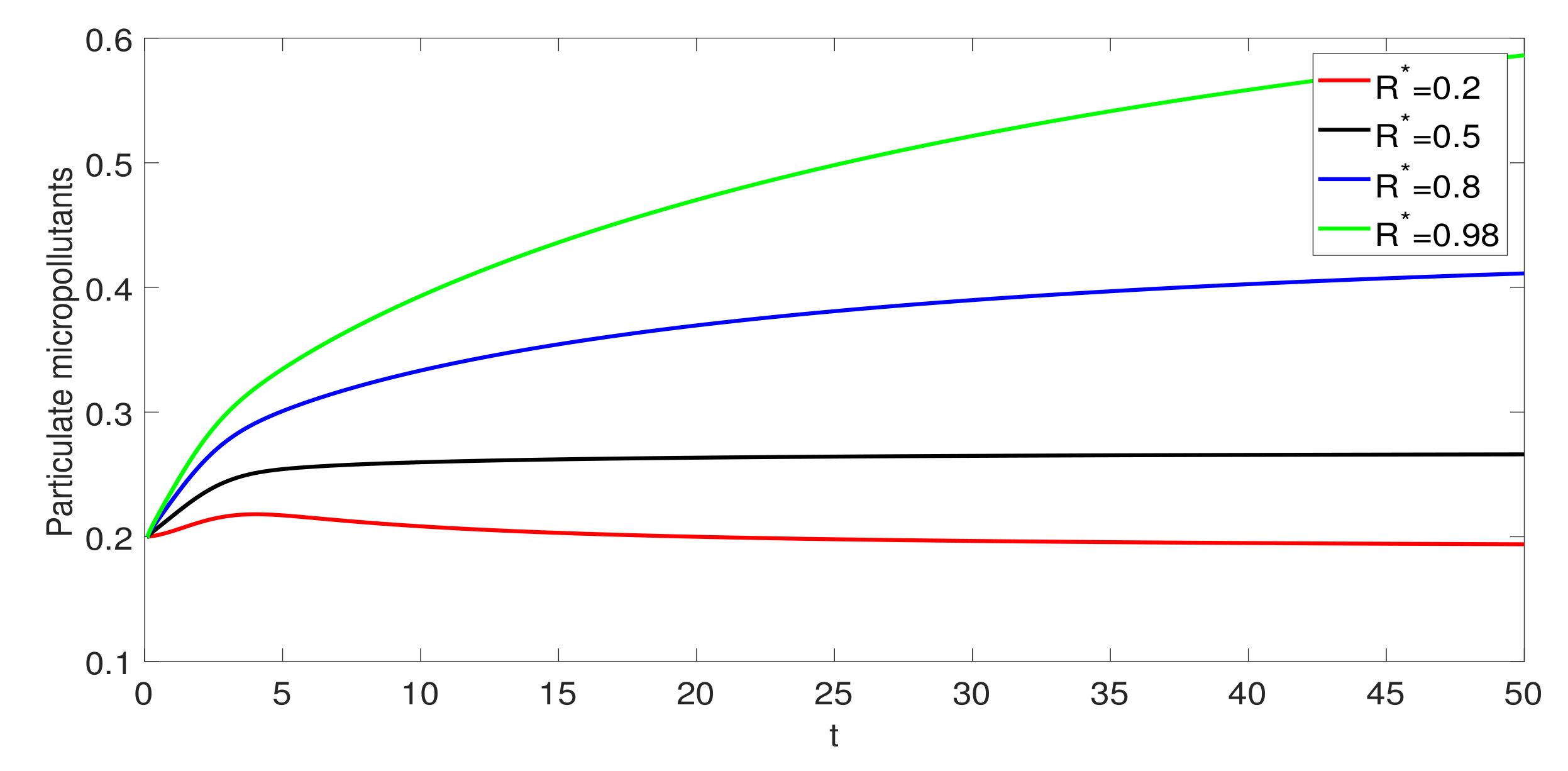
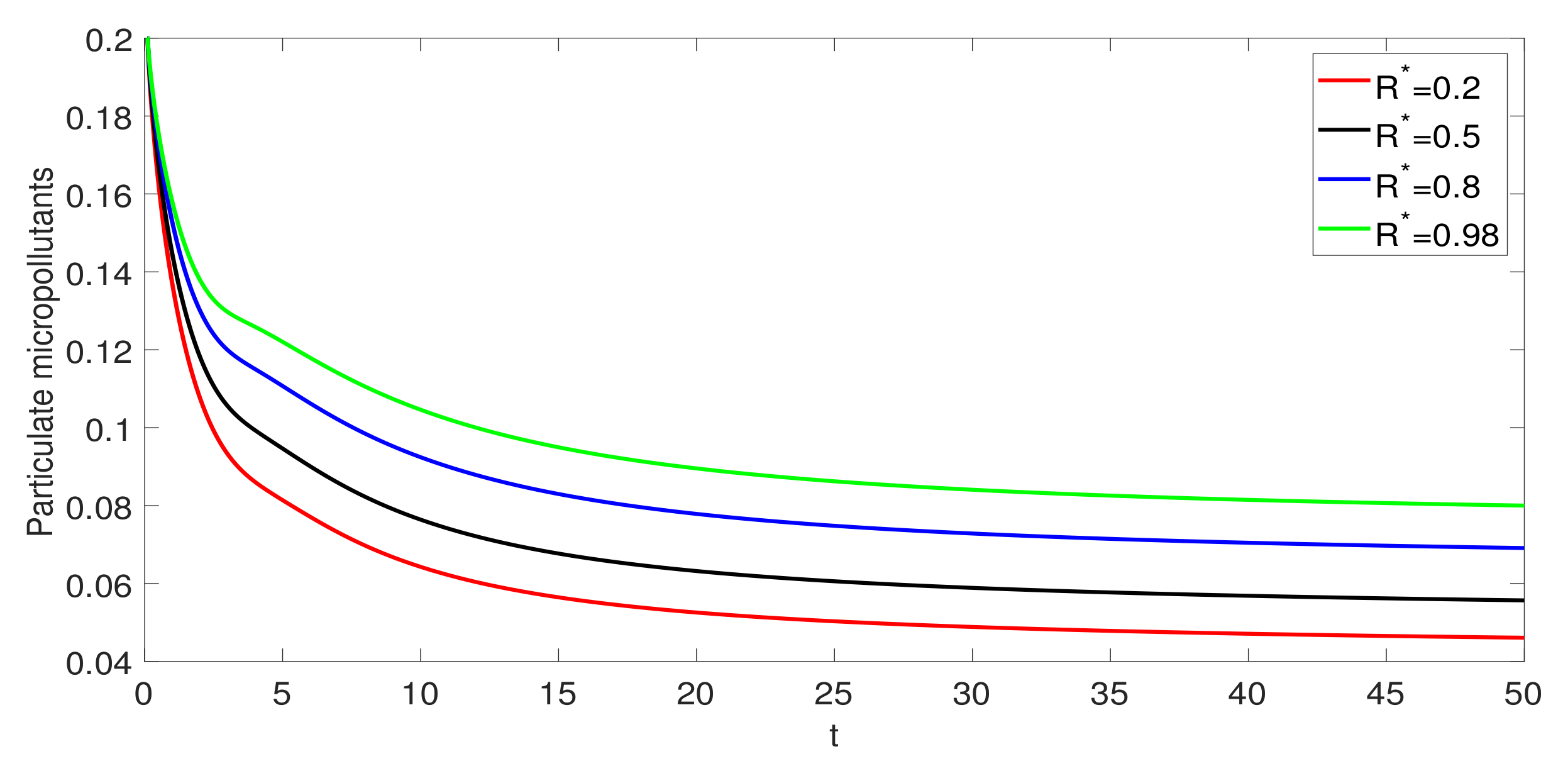
3. Numerical Simulations

In this part, we illustrate the numerical results graphically for various scenario. The parameter values used for the graphical analysis are as follows: ${\mu }_{m}ax=6$, ${\mathcal{S}}_{s,in}=0.2$, ${\mathbf{Y}}_{\mathrm{H}}=0.67$, ${\mathrm{b}}_{\mathrm{H}}=0.22$, ${\mathrm{K}}_{\mathcal{S}}=0.02$, ${\mathcal{C}}_{s,in}=100$ and ${\mathrm{c}}_2=0.9$. For the other parameters, we suggest two types of compound used for micropollutant biotransformation parameters. One is highly biodegradable and the other is slowly biodegradable compounds. The values of ${\mathrm{k}}_{sor}^{*}$, ${\mathrm{k}}_{bio}^{*}$, and ${\mathrm{k}}_d^{*}$ are given in Table 1.

Table 1. Values of for different compounds.

Compounds	${\mathbf{k}}_{\mathit{sor}}^{*}$	${\mathbf{k}}_{\mathit{bio}}^{*}$	${\mathbf{k}}_{\mathit{d}}^{*}$
Highly biodegradable
Erythromycin (ERY)	$7.23\times {10}^{-2}$	$6.03\times {10}^{-3}$	$7.1\times {10}^{-4}$
Ibuprofen (IBP)	$19.3\times {10}^{-2}$	$1.06\times {10}^{-2}$	$6.81\times {10}^{-4}$
Roxithromycin(ROX)	$47.57\times {10}^{-2}$	$9.04\times {10}^{-3}$	$1.8\times {10}^{-3}$
Naproxen(NPX)	$26.03\times {10}^{-2}$	$6.34\times {10}^{-3}$	$5.67\times {10}^{-4}$
Slowly biodegradable
Trimethoprim(TMP)	$19.4\times {10}^{-2}$	$1.43\times {10}^{-3}$	$9.11\times {10}^{-4}$
Sulfamethoxazole(SMX)	$14.97\times {10}^{-2}$	$2.06\times {10}^{-3}$	$5.8\times {10}^{-4}$
Fluoxetine(FLX)	$4.17$	$3.02\times {10}^{-3}$	$1.09\times {10}^{-2}$

The graphical illustration is discussed for the two different compounds; one is IBP and other is SMX. In Figure 1, the effect of the recycle ratio is presented for IBP and $\delta =0.8$. After an abrupt increase, it is noticed that the soluble substrate is decreasing when the recycle ratio is increasing. However, particulate biomass is increasing when the recycle ratio increases. The particulate biomass attains its maximum value at the higher value of ${\mathfrak{R}}^{*}$. It is also observed that, as the recycle ratio increases, then soluble micropollutants decrease and particulate micropollutants increase. Thus, the recycle ratio ${\mathfrak{R}}^{*}$ has an important role in the activated sludge processes. In Figure 1, the effect of the recycle ratio is presented for SMX and $\delta =0.8$. After an abrupt increase, it is noticed that the soluble substrate is decreased when the recycle ratio is increasing. However, particulate biomass is increasing when the recycle ratio increases. The particulate biomass attains its maximum value at the higher value of ${\mathfrak{R}}^{*}=0.98$. It is seen that, as the ${\mathfrak{R}}^{*}$ soluble micropollutant increases rapidly and then become stable with the passage of time, particulate micropollutants decrease. We observe different dynamics of the soluble micropullaunt and particulate micropollutants in Figure 1 and Figure 2 and because we used two different compounds for biodegradation. The IBP is highly biodegradable while SMX has low biodegradability. In Figure 3 and Figure 4, we show the effect of fractional order on the evolution of the model for IBP and SMX, respectively. As $\delta$ increases, the rate of decay or growth becomes slower, and vice versa. Thus, the fractional order $\delta$ has an important role in the rate of decay or growth process of the model.

Figure 1. Graphical illustration of the model (8) for $\delta =0.8$, IBP and various values of recycle ratio.

Figure 2. Graphical illustration of the model (8) for $\delta =0.8$, SMX and various values of recycle ratio.

Figure 3. Graphical illustration of the model (8) for IBP and various values of $\delta$.

Figure 4. Graphical illustration of the model (8) for SMX and various values of $\delta$.

4. Conclusions

In this paper, we developed a fractional-order mathematical model for the activated sludge process that incorporated the three major processes for micropollutant removal: Biological removal (biodegradation and/or cometabolism), volatilization, and sorption. We used a basic biotransformation model with no cometabolism and a rate of biodegradation that was a linear function of micropollutant concentration. We showed that the fractional order model has a non-negative solution. We calculated two steady states of solution and derived the local stability of both steady state solutions. We deduced the results that are concerned with existence of at least one solution and at most one solution of the fractional order biodegradation model through fixed point theorems of Leray–Schauder and Stephen Banach. We constructed different forms of UH stability via functional analysis. We deduced numerical results of the considered model through the Euler numerical method. We illustrated the achieved results through graphs to study the dynamics of the different classes of the considered model. The elimination of soluble micropollutants is improved when they are highly biodegradable and have a high sorption capacity, according to the results. By either raising the value of the biological degradation kinetic constant or concentrating the substrate in the feed, the limiting concentration can be reduced. Concentrating the feed improves the elimination of biodegradable pollutants. The numerical simulations shown that the recycle ratio has a great impact on the soluble and particulate micropollutants. The effect of fractional order on the evolution of the chemical process of the model has been observed. In future, one could study the considered model in different approaches:

• Most of the dynamical systems have been studied for bifurcation theory [29,30,31]. One can study the static bifurcation for the considered model.
• Using more generalized nonolocal operators with different kernels.
• Involving fuzziness and uncertainty in the model.
• Controllability and chaotic behaviour of the model.

References

- Hai, F.I.; Nghiem, L.D.; Khan, S.J.; Yamamoto, W.E.P.K. Wastewater Reuse: Removal of Emerging Trace Organic Contaminants in: Membrane Biological Reactors: Theory, Modeling, Design, Management and Applications to Wastewater Reuse; Hai, F.I., Yamamoto, K., Lee, C., Eds.; IWA: London, UK, 2014; pp. 165–205. [Google Scholar]
- Luo, Y.; Guo, W.; Ngo, H.H.; Nghiem, L.D.; Hai, F.I.; Zhang, J.; Liang, S.; Wang, X.C. A review on the occurrence of micropollutants in the aquatic environment and their fate and removal during wastewater treatment. Sci. Total Environ. 2014, 473–474, 619–641. [Google Scholar] [CrossRef] [PubMed]
- Pomies, M.; Choubert, J.-M.; Wisniewski, C.; Coquery, M. Modelling of micropollutant removal in biological wastewater treatments: A review. Sci. Total Environ. 2013, 443, 733–748. [Google Scholar] [CrossRef] [PubMed]
- Delgadillo-Mirquez, L.; Lardon, L.; Steyer, J.-P.; Patureau, D. A new dynamic model for bioavailability and cometabolism of micropollutants during anaerobic digestion. Water Res. 2011, 45, 4511–4521. [Google Scholar] [CrossRef] [PubMed]
- Criddle, C.S. The kinetics of cometabolism. Biotechnol. Bioeng. 1993, 41, 1048–1056. [Google Scholar] [CrossRef]
- Li, B.; Stenstrom, M.K. A sensitivity and model reduction analysis of one-dimensional secondary settling tank models under wet-weather flow and sludge bulking conditions. Chem. Eng. J. 2016, 288, 813–823. [Google Scholar] [CrossRef] [Green Version]
- Torfs, E.; Maere, T.; Burger, R.; Diehl, S.; Nopens, I. Impact on sludge inventory and control strategies using the benchmark simulation model no. 1 with the Burger–Diehl settler model. Water Sci. Technol. 2015, 71, 1524–1535. [Google Scholar] [CrossRef] [Green Version]
- Torfs, E.; Mart, M.C.; Locatelli, F.; Balemans, S.; Burger, R.; Diehl, S.; Laurent, J.; Vanrolleghem, P.; Francois, P.; Nopens, I. Concentration-driven models revisited: Towards a unified framework to model settling tanks in water resource recovery facilities. Water Sci. Technol. 2017, 75, 539–551. [Google Scholar] [CrossRef] [Green Version]
- Xu, G.; Yin, F.; Xu, Y.; Yu, H.-Q. A force-based mechanistic model for describing activated sludge settling process. Water Res. 2017, 127, 118–126. [Google Scholar] [CrossRef]
- Nelson, M.; Alqahtani, R.; Hai, F. Mathematical modelling of the removal of organic micropollutants in the activated sludge process: A linear biodegradation model. Anziam J. 2018, 60, 191–229. [Google Scholar] [CrossRef] [Green Version]
- Ahmad, S.; Ullah, A.; Akgül, A.; la Sen, M.D. A Novel Homotopy Perturbation Method with Applications to Nonlinear Fractional Order KdV and Burger Equation with Exponential-Decay Kernel. J. Funct. Spaces 2021, 2021, 8770488. [Google Scholar]
- Ullah, A.; Abdeljawad, T.; Ahmad, S.; Shah, K. Study of a fractional-order epidemic model of childhood diseases. J. Funct. Spaces 2020, 2020, 5895310. [Google Scholar] [CrossRef]
- Kilbas, A.; Srivastava, H.H.; Trujillo, J.J. Theory and Applications of Fractional Differential Equations; Elsevier: Amsterdam, The Netherlands, 2006. [Google Scholar]
- Caputo, M.; Fabrizio, M. A new definition of fractional derivative without singular kernel. Prog. Fract. Differ. Appl. 2015, 2015, 1–13. [Google Scholar]
- Ahmad, S.; Ullah, A.; Akgül, A.; DelaSen, M.A. study of fractional order Ambartsumian equation involving exponential decay kernel. AIMS Math. 2021, 6, 9981–9997. [Google Scholar] [CrossRef]
- Atangana, A.; Baleanu, D. New fractional derivatives with non-local and non-singular kernel: Theory and application to heat transfer model. Therm. Sci. 2016, 20, 763–769. [Google Scholar] [CrossRef] [Green Version]
- Ahmad, S.; Ullah, A.; Arfan, M.; Shah, K. On analysis of the fractional mathematical model of rotavirus epidemic with the effects of breastfeeding and vaccination under Atangana-Baleanu (AB) derivative. Chaos Solitons Fractals 2020, 140, 110233. [Google Scholar] [CrossRef]
- Ikram, M.D.; Asjad, M.I.; Akgül, A.; Baleanu, D. Effects of hybrid nanofluid on novel fractional model of heat transfer flow between two parallel plates. Alex. Eng. J. 2021, 60, 3593–3604. [Google Scholar] [CrossRef]
- Wongcharoen, A.; Ntouyas, S.K.; Tariboon, J. Boundary Value Problems for Hilfer Fractional Differential Inclusions with Nonlocal Integral Boundary Conditions. Mathematics 2020, 8, 1905. [Google Scholar] [CrossRef]
- Abdo, M.S.; Saeed, A.M.; Panchal, S.K. Panchal, Existence and Ulam–Hyers–Mittag–Leffler stability results of Ψ-Hilfer nonlocal Cauchy problem. Rend. Circ. Mat. 2021, 2, 57–77. [Google Scholar]
- Liu, K.; Feckan, M.; Wang, J. Hyers–Ulam Stability and Existence of Solutions to the Generalized Liouville–Caputo Fractional Differential Equations. Symmetry 2020, 12, 955. [Google Scholar] [CrossRef]
- Ahmed, I.; Kumam, P.; Abubakar, J.; Borisut, P.; Sitthithakerngkiet, K. Solutions for impulsive fractional pantograph differential equation via generalized anti-periodic boundary condition. Adv. Diff. Equ. 2020, 2020, 1–15. [Google Scholar]
- Hinze, M.; Schmidt, A.; Leine, R.I. Numerical solution of fractional-order ordinary differential equations using the reformulated infinite state representation. Fract. Calc. Appl. Anal. 2019, 22, 1321–1350. [Google Scholar] [CrossRef]
- Alqahtani, R.T.; Ahmad, S.; Akgül, A. Dynamical Analysis of Bio-Ethanol Production Model under Generalized Nonlocal Operator in Caputo Sense. Mathematics 2021, 9, 2370. [Google Scholar] [CrossRef]
- Qureshi, S.; Yusuf, A.; Shaikh, A.A.; Inc, M.; Baleanu, D. Fractional modeling of blood ethanol concentration system with real data application. Chaos 2019, 29, 013143. [Google Scholar] [CrossRef]
- Panjwani, S.; Tejaswini, E.S.S.; Rao, A.S. Fractional Order Model-Based Design of Controllers for Improved Operation of Wastewater Treatment Plants. Trans. Indian Natl. Acad. Eng. 2020, 5, 719–726. [Google Scholar] [CrossRef]
- Barbu, M.; Ceanga, E. Fractional order controllers for urban wastewater treatment systems. In Proceedings of the 23rd Mediterranean Conference on Control and Automation (MED), Malaga, Spain, 16–19 June 2015; pp. 1174–1179. [Google Scholar]
- El-Seddik, M.M. Modified Fractional-Order Activated Sludge Model (MFASM) for Aerobic Microbial Growth in Wastewater. Inorg. Chem. Ind. J. 2017, 12, 1–8. [Google Scholar]
- Sidorov, N.; Sidorov, D.; Sinitysn, A. Toward General Theory of Differential-Operator and Kinetic Models; World Scientific Series on Nonlinear Science Series A; Chua, L., Ed.; World Scientific: Singapore; London, UK, 2020. [Google Scholar]
- Vainberg, M.M.; Trenogin, V.A. Theory of Branching of Solutions of Non-linear Equations, Noordhoff. 1974. Available online: https://www.abebooks.com/Theory-Branching-Solutions-Nonlinear-Equations-Monographs/22683271746/bd (accessed on 2 October 2021).
- Trenogin, V.A.; Sidorov, N.A. An investigation of the bifurcation points and nontrivial branches of the solutions of nonlinear equations. Differ. Integral Equ. 1972, 1, 216–247. [Google Scholar]
Publisher’s Note: MDPI stays neutral with regard to jurisdictional claims in published maps and institutional affiliations. |
© 2021 by the authors. Licensee MDPI, Basel, Switzerland. This article is an open access article distributed under the terms and conditions of the Creative Commons Attribution (CC BY) license (https://creativecommons.org/licenses/by/4.0/).