Abstract
This paper proposes a robust tracking control method for swing-up and stabilization of a rotational inverted pendulum system by applying equivalent input disturbance (EID) rejection. The mathematical model of the system was developed by using a Lagrangian equation. Then, the EID, including external disturbances and parameter uncertainties, was defined; and the EID observer was designed to estimate EID using the state observer dynamics and a low-pass filter. For robustness, the linear-quadratic regulator method is used with EID rejection. The closed-loop stability is proven herein using the Lyapunov theory and input-to-state stability. The performance of the proposed method is validated and verified via experimental results.
1. Introduction
The rotational inverted pendulum (RIP) is a typical underactuated system in which the number of actuators is less than the system’s degrees of freedom [1]. The inverted pendulum system consists of a translating base and an attached pendulum without an actuator. The RIP has a motor as the rotational actuator, which provides torque to the motor’s rod [2]. Generally, the control objectives of the RIP are as follows: swing-up control, stabilizing control, and trajectory tracking control [3,4,5]. Currently, control methods for the RIPs are being extensively used in various fields, such as spacecraft attitude control [6], biped robot balance control [7,8], vehicle and vessel self-balanced control [9,10], and flight control [11,12]. However, it is difficult to control the RIP because of limitations such as the unstable equilibrium point, and nonlinearities, including the state couple terms of the arm angle, velocity, the pole angle and velocity, and sine functions.
Various control methods have been proposed to overcome these issues. Proportional-integral-derivative (PID) control has been widely used owing to its simple design, low maintenance cost, and effectiveness in various systems [13]. However, its control performance may degrade under the disturbances. Linear-quadratic regulator (LQR) control methods have been applied to RIP control to improve the robustness and optimal performance [14,15]. A fuzzy-based control method was also developed for the RIP [16]. The aforementioned methods may be unstable and degraded owing to parameter uncertainties and/or external disturbance, because the parameter uncertainties and/or external disturbance were not considered in the controller design.
Sliding mode control (SMC) methods for RIP were designed for robustness [17,18]. However, the chattering phenomenon caused by SMC may degrade the control performance. To reduce the chattering, the adaptive sliding mode based disturbance attenuation tracking control method and extended state observer based adaptive sliding mode tracking control were proposed for wheeled mobile robots [19,20]. However, these methods cannot be applied to the RIP due to the differences between wheeled mobile robots and the RIP. Adaptive control methods have been used to overcome parameter uncertainties [21,22]. However, the parameters may be poorly estimated for the rapidly varying parameters. Furthermore, the disturbance can affect the stability. Disturbance observer (DOB) methods can be used to compensate for the effects of disturbances [23,24]. In the DOB design, the main concern is that the DOB is available when the system satisfies the matching condition. However, the disturbance in the RIP does not satisfy the matching condition. Furthermore, it is difficult to reject the disturbances caused by the single control input in the RIP; thus, the DOB cannot be applied to the RIP. To overcome this problem, equivalent input disturbance (EID) was proposed in [25]. In this paper, only external disturbance was considered. Furthermore, to the best of our knowledge, the EID was not designed for the arm angle tracking control with pole balancing in the RIP.
In this paper, we propose an arm angle tracking control method with pole balancing using the EID rejection for the RIP. The proposed method consists of a state observer, an EID observer, and a state feedback controller. The EID rejection method is proposed to reject the disturbances that do not satisfy the matching condition because the RIP is the underactuated system. The state observer and EID observer were developed to estimate the EID, which is equivalent to the disturbances. The states are estimated using the state observer. Then, the EID observer generates the estimated EID using the estimated state. The desired state dynamics are derived using the system model. For arm angle tracking control and pole balancing with disturbance compensation, a state feedback controller was designed using the desired state dynamics. The control gains are selected using the LQR method to obtain the optimal control performance. Consequently, the proposed method is robust against the disturbance not satisfying the matching condition, although the RIP is the underactuated system. The closed-loop stability is proven via Lyapunov theory and input-to-state stability (ISS). The performance of the proposed method was validated experimentally.
2. System Modeling
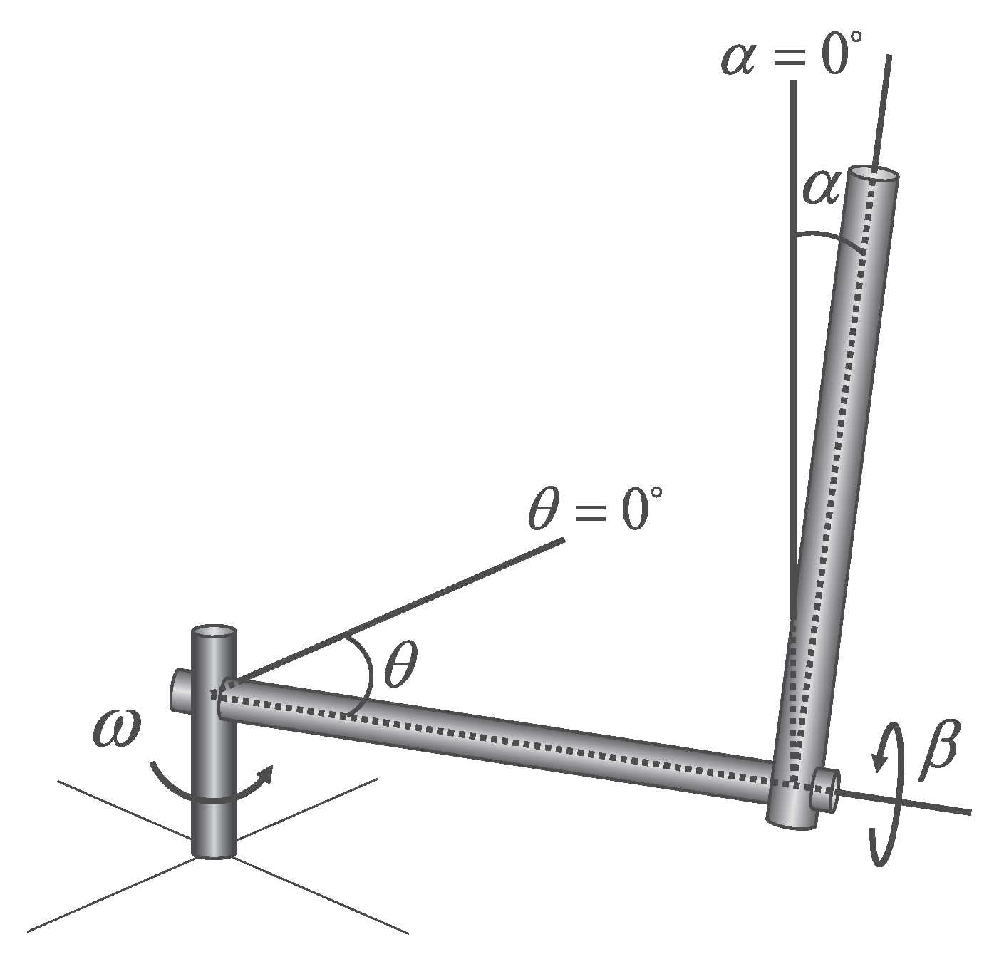
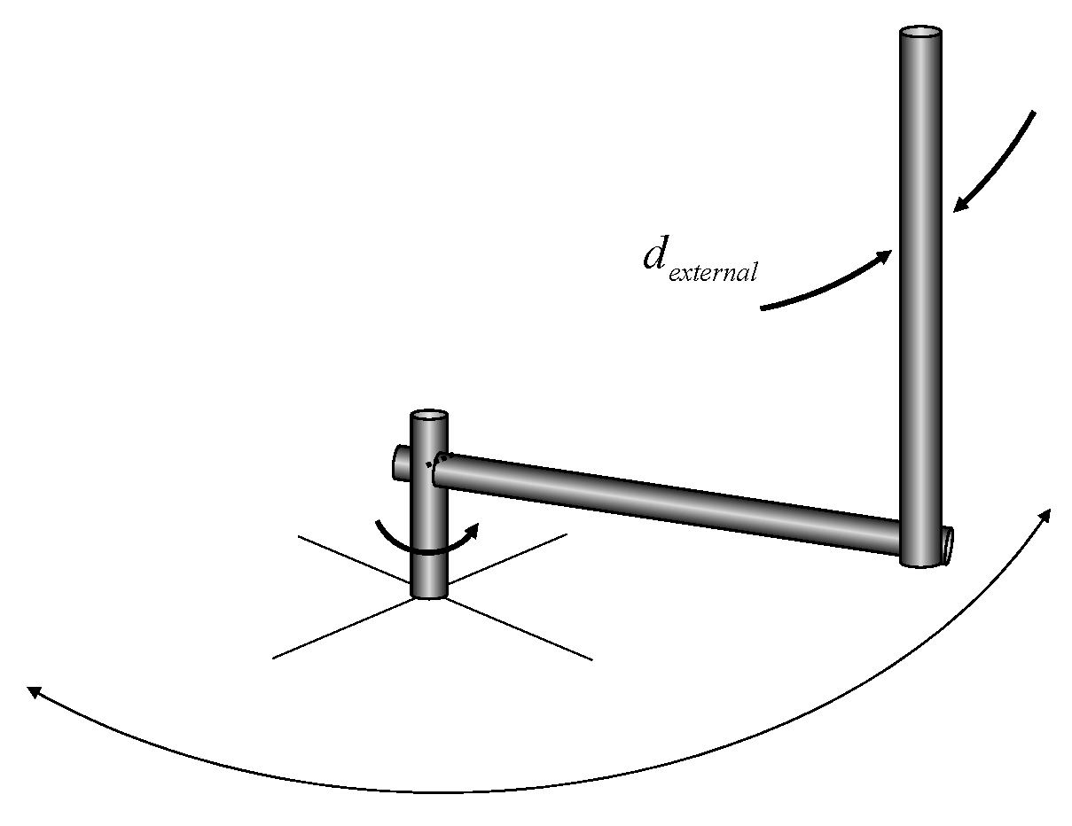
Figure 1 shows a simplified schematic model of the RIP. is the arm angle, is the pendulum pole angle, is the arm angular velocity, and is the pendulum pole angular velocity. The system model can be obtained by solving the Euler–Lagrange Equation [3,26]. The Lagrangian is defined as the difference between the kinetic energy () and potential energy (). For the RIP, can be defined as
where is a velocity of the center of the mass of the pendulum, is the rotary arm (motor rod) inertia, is the pendulum inertia, is the pendulum mass, is the pendulum length, and g is the gravitational acceleration. can be obtained by time-differentiating the pendulum center position . The pendulum center position is calculated as follows:
Then, and is calculated as follows:
where is the rotary arm length.
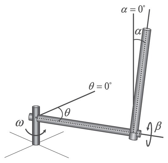
Figure 1.
Simplified schematic model of the RIP.
For the RIP, the Euler–Lagrange equation is formulated as
For DC motor torque , it can be replaced as . Thus, the Euler–Lagrange Equation (4) can be rewritten as:
where is the DC motor torque constant, R is the DC motor terminal resistance, and is the motor input voltage. In this paper, the main goal of the controller design is arm angle tracking control with the balancing control (). Thus, at the operating point , the RIP model (5) can be linearized as
The state-space equation is derived from (6), and rewritten as follows:
where , , , , , and .
3. EID Estimator Design
In the system model described in (7), disturbances, such as friction, are not considered. Considering the external disturbances, the system model becomes
where , , and are the disturbances in the dynamics of and , respectively. In practice, it is difficult to determine the disturbances, and , because these disturbances may include friction, modeling uncertainties, and/or parameter uncertainties. Furthermore, these disturbances cannot be rejected by a single input because and are in the dynamics of and . To resolve this issue, an EID rejection method is proposed for the RIP. The equivalent system model from (8) is defined as
where is defined as the EID which induces the same effect as and on the system. We assume that the control input is . is defined as the output of the plant (8) for the zero input and the disturbances . Furthermore, is defined as the output of the plant (9) for the zero input and the disturbance . The disturbance is called the EID of the disturbances and if for all .
First, a state observer is designed to estimate the EID. The estimation for x is defined as . The state observer is designed as
where L is the observer gain matrix, and is the control input without the EID rejection. The estimation error of the state is defined as . From (9) and (10), the dynamics of can be expressed as
The dynamics of in (11) can be rewritten as
We assume that there exists a control input such that
The estimated EID is defined as
Then, (10) becomes
Applying (13) and (14) to (12), the estimated EID can be obtained using the EID observer as follows:
where is the pseudo-inverse matrix of B. To avoid the algebraic error in (15) and (16), the estimated EID is filtered using a first-order low-pass filter as follows:
Thus, the actual control input is
The dynamics of is defined as
In (19), we assume that exists such that . The estimation error of the EID is defined as
Then the state and the EID estimation error dynamics are obtained as
Observer and EID estimation error dynamics (21) can be rewritten as
Theorem 1.
Consider the observer and EID estimation error dynamics in (22). If the observer gain matrix L is chosen such that is Hurwitz, then is globally uniformly ultimately bounded.
Proof.
We define the Lyapunov candidate function as
The derivative of with respect to time is
For
Thus is globally uniformly ultimately bounded. □
4. LQR Based Tracking Controller Design
In this section, an arm position tracking controller with pivot balancing is designed. The desired state is defined as
where , , , and are the desired values (or trajectories) of , , , and , respectively. From (7), the dynamics of are given by
where is the desired input for . In , , and can be arbitrarily chosen. From (27), we obtain
In (27), the dynamics of and can be rewritten as
Thus, from (29), the desired input is calculated as
where is the pseudo-inverse matrix of . The tracking error e is defined as follows.
From (7) and (27) the error dynamics are obtained as
The error dynamics in (32) can be rewritten as
The state feedback controller is designed as
where K is the control gain matrix. The control gain matrix K is chosen using the LQR. The objective function J is defined as
where , Q is the diagonal weighting matrix of state e, and R is the weighting factor of . From the algebraic Riccati equation:
where P is positive definite symmetric matrix. The LQR control gain vector K is obtained as
where . Using the controller in (34), the error dynamics in (32) become
From now on, we study the stability of the closed-loop system, including the error dynamics in (38) and estimation error dynamics in (21). In the controller described in (34), the estimated state is used instead of x. Thus, from the error dynamics in (38) and estimation error dynamics in (21), the closed-loop system is obtained as
Theorem 2.
Consider the closed-loop system from (39). If the control gain matrix K and observer gain L are chosen such that and are Hurwitz, respectively, then e, , and are globally uniformly ultimately bounded.
Proof.
The closed-loop system from (39) can be rewritten as
In Theorem 1, it was shown that is globally uniformly ultimately bounded if the observer gain L is selected such that is Hurwitz. In (40), if the control gain matrix K is chosen such that is Hurwitz, the dynamics of e are input-to-state stable. Thus, e is also globally uniformly ultimately bounded. Consequently, we conclude that e, , and are globally uniformly ultimately bounded. □
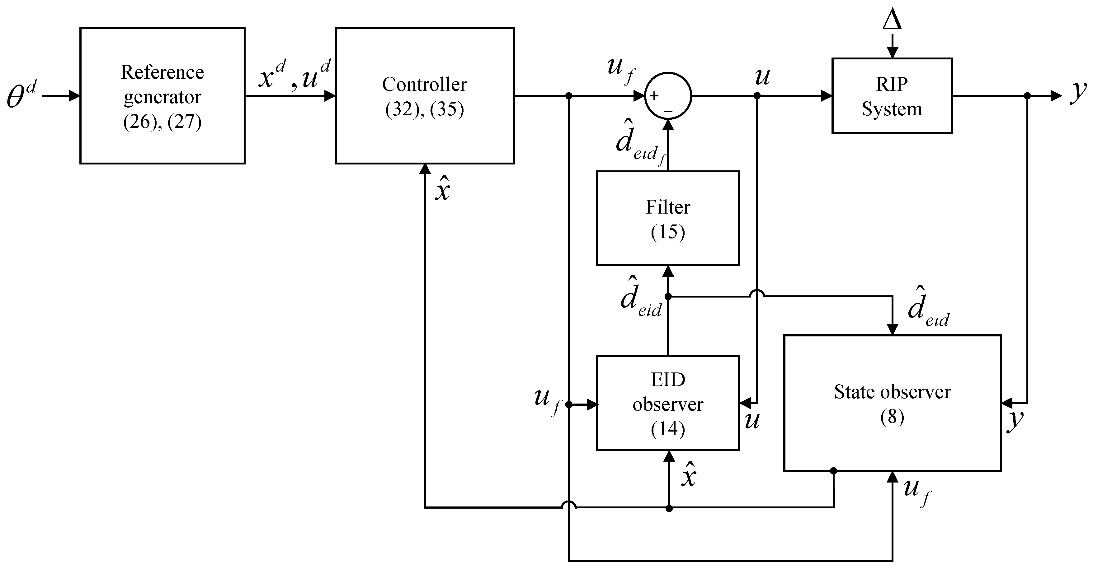
Figure 2 shows a block diagram of the proposed method. The desired state and desired input are calculated using the reference generator from (26) and (27). The state observer from (8) estimates the state; then, the EID observer from (14) generates . is obtained via the filter from (15), and is obtained using the controller from (32) and (35). Finally, the control input u was generated using and .
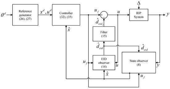
Figure 2.
Block diagram of the proposed method.
5. Experimental Results
Experiments were conducted to validate the performance of the proposed method. For the experiments, Quanser QUBE-Servo 2 with a pendulum [27] was used. Two optical incremental encoders with a resolution of 2048 pulses/rev were used to measure and . The sampling rate was set to 1 kHz.
The parameters considered in the experiments have been listed in Table 1. In the experiments, first, the proportional feedback swing-up control method [28] was used. Then when rad, the application of the proposed method for balancing started at . The motor arm position reference was used as . For balancing control, the desired pole angle was . The controller and observer gains used in the experiments were as follows: , , , , , , , , , , , and . For the low pass filter, was used.

Table 1.
System parameters.
5.1. Performances of Arm Angle Tracking Control and Pole Balancing
In the experiments, three cases were tested to validate the control performance and the EID compensation performance as follows:
- Case 1: Conventional proportional-derivative (PD) controller,
- Case 2: Proposed method without EID compensation,
- Case 3: Proposed method with EID compensation, .
- Case 3: Proposed method with EID compensation under the parameter uncertainties (at most, ±20%), .
Case 1 was tested to validate the performances of the arm angle tracking control and the pole balancing of the proposed method. Case 2 was tested to validate the performance of the EID compensation. Cases 3 and 4 were tested to validate the robustness of the proposed method.
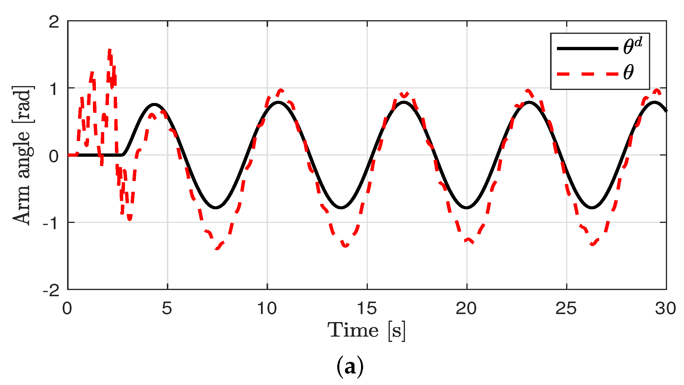
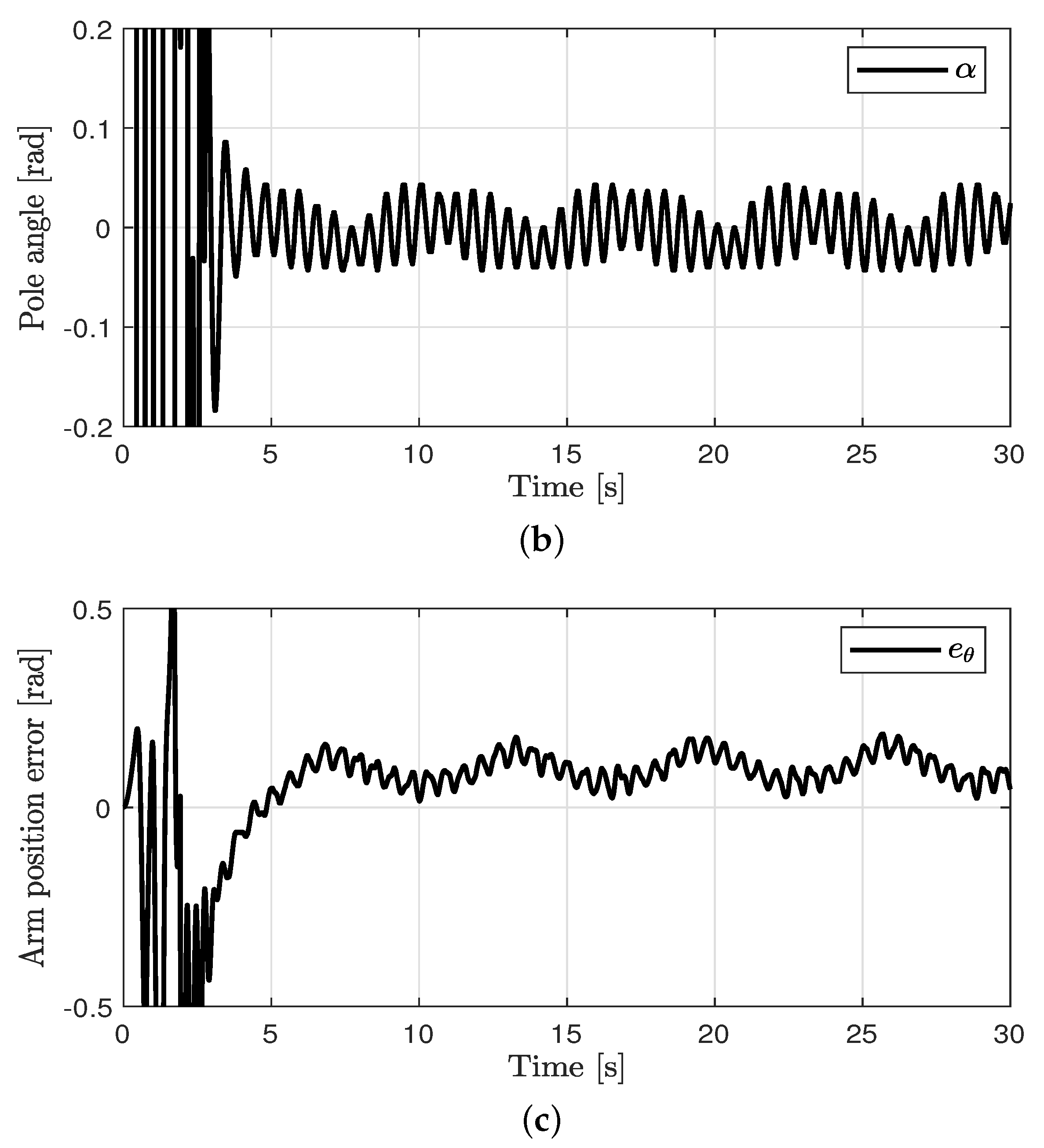
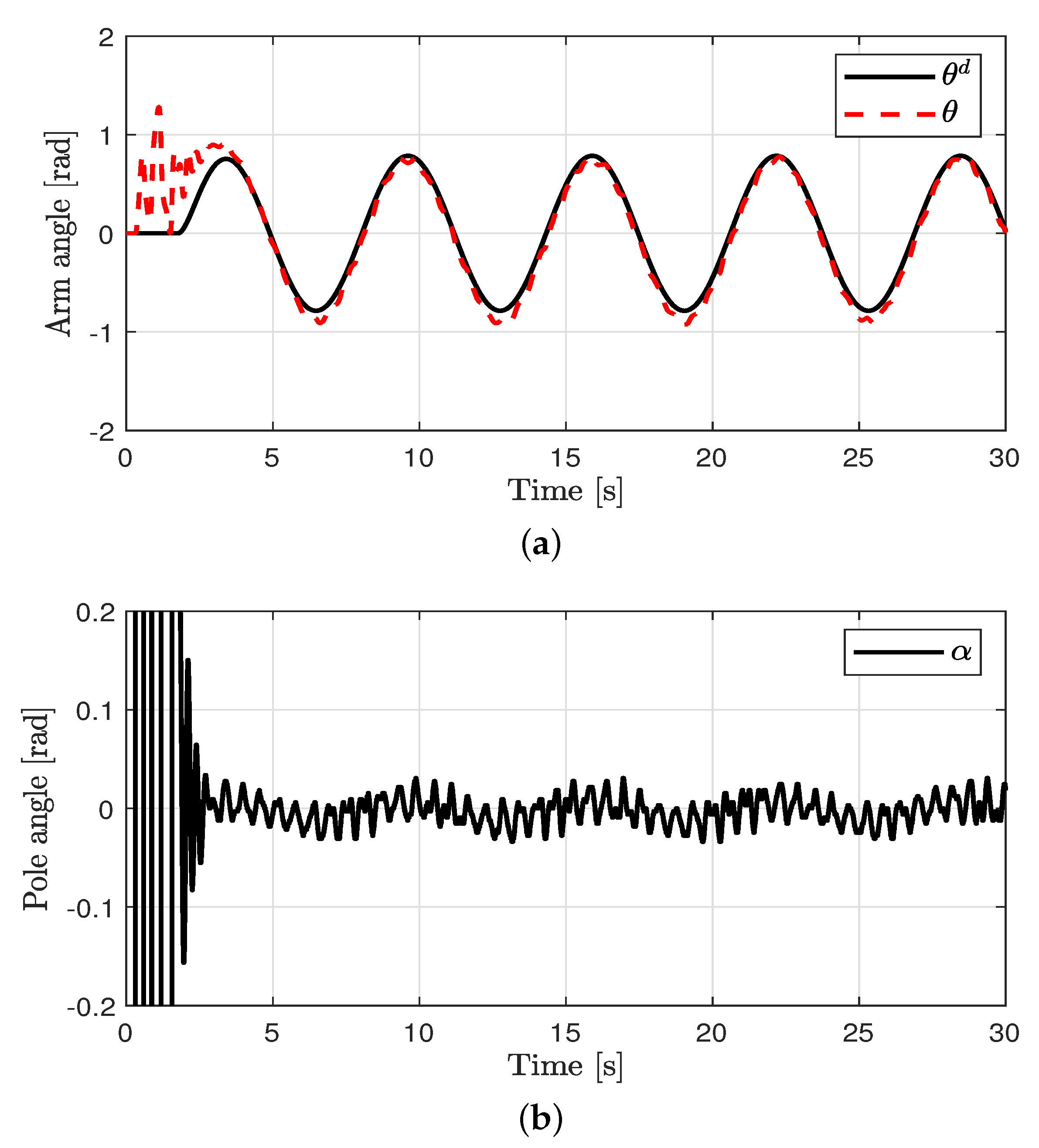
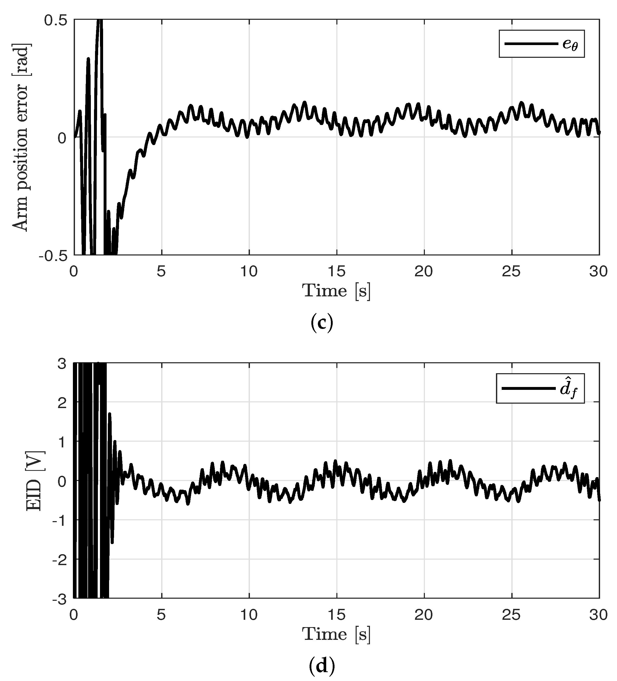
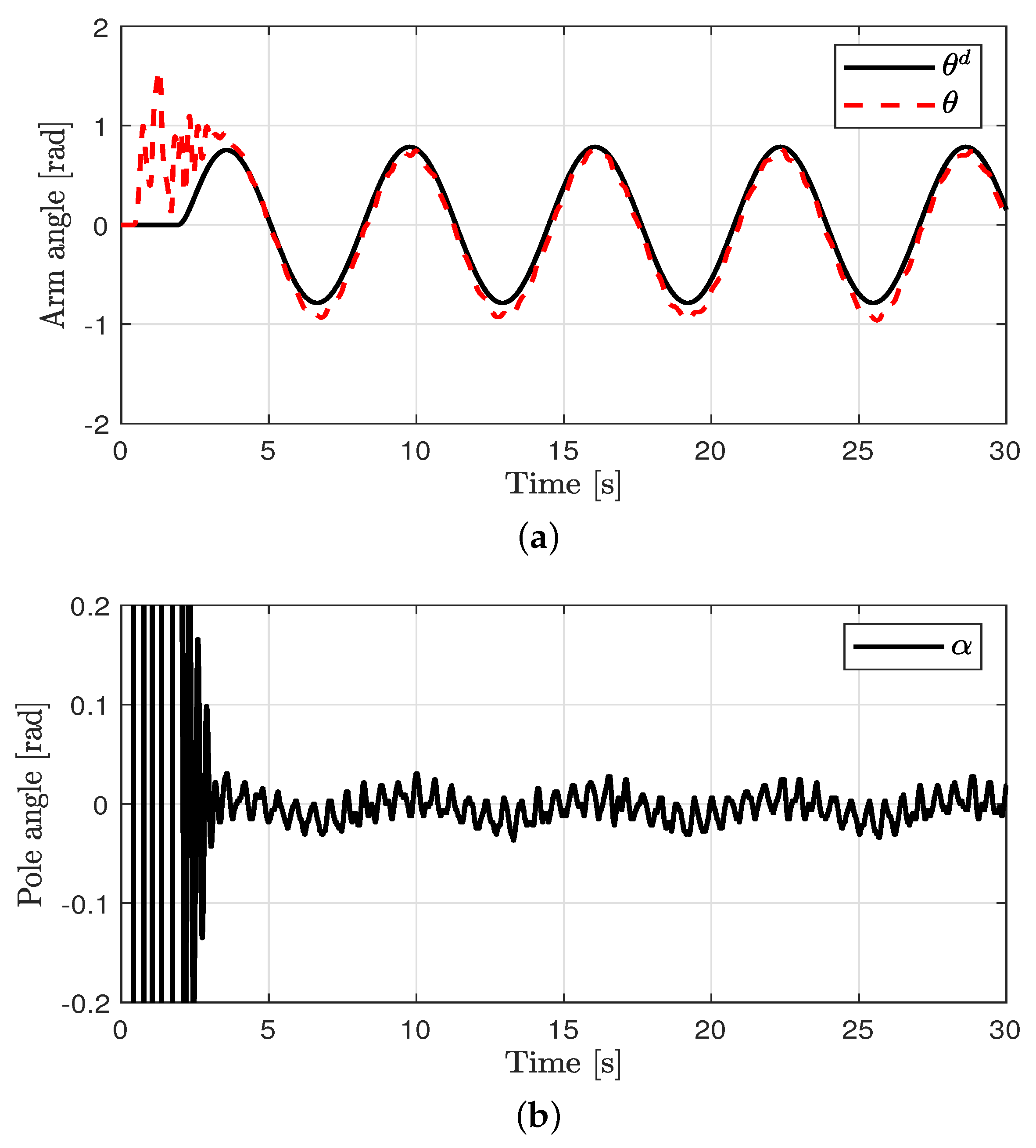
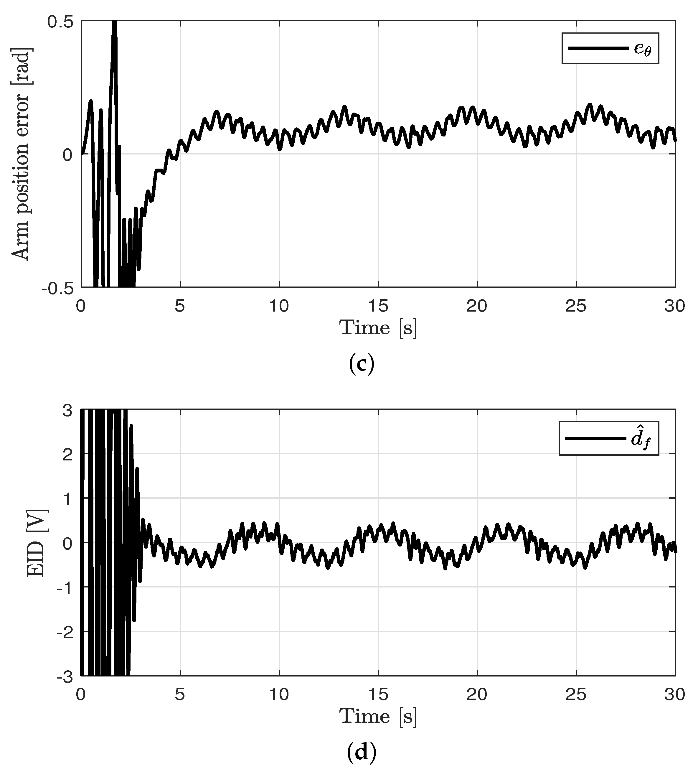
Tracking control for the arm angle and balance control for the pole angle were performed. The control performances in all cases are shown in Figure 3, Figure 4, Figure 5 and Figure 6. The oscillations in all cases were the results of the swing-up control at the outset. After rad was attained, the proposed method was applied to achieve the tracking control for the arm angle and balance control for the pole angle. The unavoidable ripple appeared owing to the quantization effect, physical coupling effect, mechanical vibration, and model uncertainty. The offset errors in the arm position tracking existed owing to the physically connected encoder wire. In case 1, relatively large errors in the arm angle and pole angle appeared because of the disturbances. In case 2, the errors were reduced by the proposed control method compared to the PD controller. In case 3, the EID compensation resulted in reduced errors compared to case 2. In case 4, the parameter uncertainties (at most, ±20%) were applied in the proposed method. Although the parameter uncertainties were applied in case 4, the control performances of cases 3 and 4 were similar.
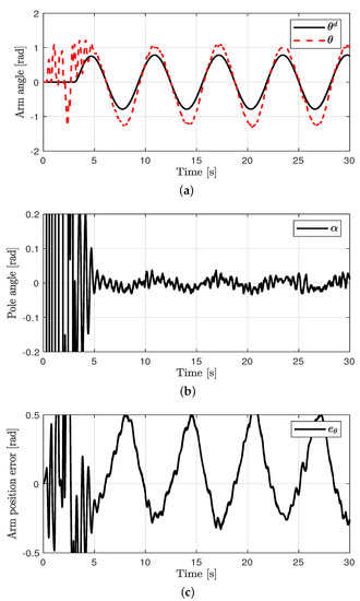
Figure 3.
Control performance in case 1. (a) Arm position (case 1). (b) Pendulum pole position (case 1). (c) Arm position error (case 1).
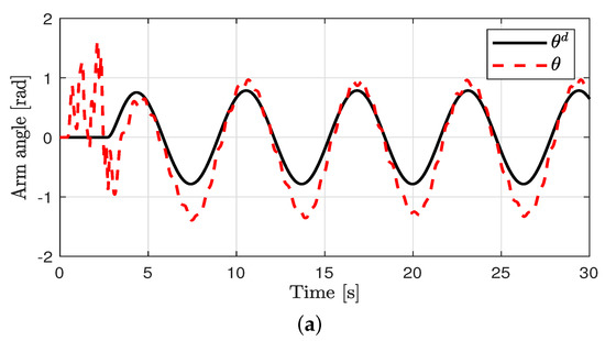
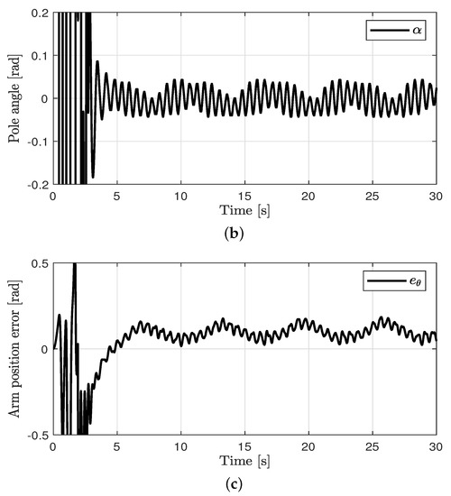
Figure 4.
Control performance in case 2. (a) Arm position (case 2). (b) Pendulum pole position (case 2). (c) Arm position error (case 2).
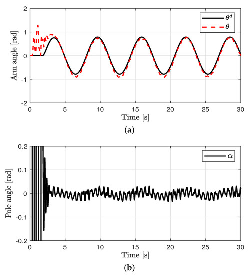
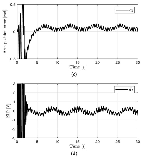
Figure 5.
Control performance in case 3. (a) Arm position (case 3). (b) Pendulum pole position (case 3). (c) Arm position error (case 3). (d) Estimated EID (case 3).


Figure 6.
Control performance in case 4. (a) Arm position (case 4). (b) Pendulum pole position (case 4). (c) Arm position error (case 4). (d) Estimated EID (case 4).
For the comparison of the control performances of all cases, the average squared error (ASE) [29] was used as follows:
where N is the number of samples. The ASE for all cases are listed in Table 2. We see that the proposed method improved the performances of the tracking control for the arm angle and balance control for the pole angle.
Table 2.
ASE for all cases.
5.2. Robustness against External Disturbance
The experiments under external disturbance were tested to validate the robustness performance of the proposed method against the external disturbance. The impulse external disturbance as shown in Figure 7 was injected by hand twice times at 9 s and 15 s in the RIP. The control performance of the proposed method under the external disturbance is shown in Figure 8. Due to the impulse external disturbance injections at 9 s and 15 s, the oscillations appeared. After the impulse external disturbance injections, the errors converged to zeros by the proposed method rapidly.

Figure 7.
External disturbance in the experiments.
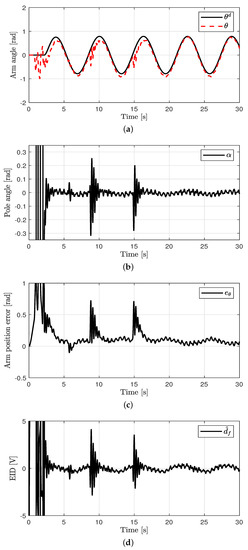
Figure 8.
Control performance of the proposed method under the external disturbance. (a) Arm position (case 4). (b) Pendulum pole position (case 4). (c) Arm position error (case 4). (d) Estimated EID (case 4).
6. Conclusions
In this study, we developed a position tracking control method with EID rejection for RIP. The system model was developed by using Lagrangian equation and was linearized at the operation point. Additionally, the EID was defined and designed. It contains the external disturbances and parameter uncertainties. The EID was estimated using a state observer, and filtered via a low-pass filter. The state error was defined with state feedback, and for position reference tracking, desired state dynamics were obtained. The tracking controller was designed using the LQR method. The stability of EID dynamics was proven by the Lyapunov theory, and the tracking error dynamics satisfied the ISS. The proposed method was validated through experiments. The main drawbacks of the proposed method are the filtering error and input saturation problems. Thus, in the future works, we will design the RIP control method to resolve these problems [29,30,31].
Author Contributions
H.L. and W.K. designed the algorithm and developed the simulation; J.G. and S.Y. provided guidance in designing the algorithm; Y.G. verified the simulation model and results. All authors have read and agreed to the published version of the manuscript.
Funding
This work was supported in part by the Energy Cloud Research and Development Program through the National Research Foundation of Korea (NRF) funded by the Ministry of Science, ICT under Grant 2019M3F2A1073313, and in part by the Climate Change Response Technology Development Program through the National Research Foundation of Korea (NRF) funded by the Ministry of Science, ICT under Grant 2021M1A2A2065445.
Institutional Review Board Statement
Not applicable.
Informed Consent Statement
Not applicable.
Data Availability Statement
Not applicable.
Conflicts of Interest
The authors declare that they have no conflict of interest.
References
- Spong, M.W. Underactuated mechanical systems. In Control Problems in Robotics and Automation; Springer: Berlin/Heidelberg, Germany, 1998; pp. 135–150. [Google Scholar]
- Awtar, S.; King, N.; Allen, T.; Bang, I.; Hagan, M.; Skidmore, D.; Craig, K. Inverted pendulum systems: Rotary and arm-driven-a mechatronic system design case study. Mechatronics 2002, 12, 357–370. [Google Scholar] [CrossRef]
- Furuta, K.; Yamakita, M.; Kobayashi, S. Swing up control of inverted pendulum. Proc. Int. Conf. Ind. Electron. Control Instrum. 1991, 206, 263–269. [Google Scholar]
- Mathew, N.; Rao, J.; Koteswara, K.; Sivakumaran, N. Swing up and stabilization control of a rotary inverted pendulum. IFAC Proc. Vol. 2013, 46, 654–659. [Google Scholar] [CrossRef] [Green Version]
- Yang, X.; Zheng, X. Swing-up and stabilization control design for an underactuated rotary inverted pendulum system: Theory and experiments. IEEE Trans. Ind. Electron. 2018, 65, 7229–7238. [Google Scholar] [CrossRef]
- Chen, T.; Shan, J.; Wen, H. Distributed adaptive attitude control for networked underactuated flexible spacecraft. IEEE Trans. Aerosp. Electron. Syst. 2018, 55, 215–225. [Google Scholar] [CrossRef]
- Chevallereau, C.; Grizzle, J.W.; Shih, C.L. Asymptotically stable walking of a five-link underactuated 3-D bipedal robot. IEEE Trans. Robot. 2009, 25, 37–50. [Google Scholar] [CrossRef] [Green Version]
- Chignoli, M.; Wensing, P.M. Variational-based optimal control of underactuated balancing for dynamic quadrupeds. IEEE Access 2000, 8, 49785–49797. [Google Scholar] [CrossRef]
- Ashrafiuon, H.; Nersesov, S.; Clayton, G. Trajectory tracking control of planar underactuated vehicles. IEEE Trans. Automat. Control 2017, 62, 1959–1965. [Google Scholar] [CrossRef]
- Tu, F.; Ge, S.S.; Choo, Y.S.; Hang, C.C. Adaptive dynamic positioning control for accommodation vessels with multiple constraints. IET Control Theory Appl. 2017, 11, 329–340. [Google Scholar] [CrossRef]
- Huang, X.; Yan, Y. Saturated backstepping control of underactuated spacecraft hovering for formation flights. IEEE Trans. Aerosp. Electron. Syst. 2017, 53, 1988–2000. [Google Scholar] [CrossRef]
- Tao, Q.; Wang, J.; Xu, Z.; Lin, T.X.; Yuan, Y.; Zhang, F. Swing-Reducing Flight Control System for an Underactuated Indoor Miniature Autonomous Blimp. IEEE/ASME Trans. Mechatron. 2021. [Google Scholar] [CrossRef]
- Johnson, M.A.; Moradi, M.H. PID Control; Springer: London, UK, 2005. [Google Scholar]
- Hazem, Z.B.; Fotuhi, M.J.; Bingül, Z. Development of a fuzzy-LQR and fuzzy-LQG stability control for a double link rotary inverted pendulum. J. Franklin Inst. 2020, 357, 10529–10556. [Google Scholar] [CrossRef]
- Saleem, O.; Mahmood-Ul-Hasan, K. Indirect adaptive state-feedback control of rotary inverted pendulum using self-mutating hyperbolic-functions for online cost variation. IEEE Access 2020, 8, 91236–91247. [Google Scholar] [CrossRef]
- Eini, R.; Abdelwahed, S. Indirect Adaptive fuzzy Controller Design for a Rotational Inverted Pendulum. In Proceedings of the 2018 Annual American Control Conference, Milwaukee, WI, USA, 27–29 June 2018; pp. 1677–1682. [Google Scholar]
- Park, M.-S.; Chwa, D. Swing-up and stabilization control of inverted-pendulum systems via coupled sliding-mode control method. IEEE Trans. Ind. Electron. 2009, 56, 3541–3555. [Google Scholar] [CrossRef]
- Nguyen, N.P.; Oh, H.; Kim, Y.; Moon, J.; Yang, J.; Chen, W.H. Fuzzy-based super-twisting sliding mode stabilization control for under-actuated rotary inverted pendulum systems. IEEE Access 2020, 8, 185079–185092. [Google Scholar] [CrossRef]
- Kang, L.; Hongbo, G.; Haibo, J.; Zhengyuan, H. Adaptive sliding mode based disturbance attenuation tracking control for wheeled mobile robots. Int. J. Control Automat. Syst. 2020, 18, 1288–1298. [Google Scholar]
- Kang, L.; Haibo, J.; Yinuo, Z. Extended state observer based adaptive sliding mode tracking control of wheeled mobile robot with input saturation and uncertainties. Proc. Ins. Mech. Eng. Part C J. Mech. Eng. Sci. 2019, 233, 5460–5476. [Google Scholar]
- Rudra, S.; Ranjit, K.B. Robust adaptive backstepping control of inverted pendulum on cart system. Int. J. Control Automat. 2012, 5, 13–26. [Google Scholar]
- Rahmani, R.; Mobayen, S.; Fekih, A.; Ro, J.-S. Robust passivity cascade technique-based control using RBFN approximators for the stabilization of a cart inverted pendulum. Mathematics 2021, 9, 1229. [Google Scholar] [CrossRef]
- Won, D.; Kim, W.; Shin, D.; Chung, C.C. High gain disturbance observer based backstepping control with output tracking error constraint for electro-hydraulic systems. IEEE Trans. Control Syst. Technol. 2015, 23, 787–795. [Google Scholar] [CrossRef]
- Kim, W.; Suh, S. Optimal disturbance observer design for high tracking performance in motion control systems. Mathematics 2020, 8, 1633. [Google Scholar] [CrossRef]
- Jin-Hua, S.; Mingxing, F.; Yasuhiro, O.; Hiroshi, H.; Min, W. Improving disturbance-rejection performance based on an equivalent-input-disturbance approach. IEEE Trans. Ind. Electron. 2008, 55, 380–389. [Google Scholar] [CrossRef]
- Wang, J.J. Simulation studies of inverted pendulum based on PID controllers. Simul. Model. Pract. Theory 2011, 19, 440–449. [Google Scholar] [CrossRef]
- Quanser User Mannual. Available online: https://quanserinc.box.com/shared/static/jewhkc82kbgng0la81mx74dilriv4dw0.zip (accessed on 28 August 2021).
- Åström, K.J.; Furuta, K. Swinging up a pendulum by energy control. Automatica 2000, 36, 287–295. [Google Scholar] [CrossRef] [Green Version]
- Kang, L.; Rujing, W.; Xiaodong, W.; Xingxian, W. Anti-saturation adaptive finite-time neural network based fault-tolerant tracking control for a quadrotor UAV with external disturbances. Aerosp. Sci. Technol. 2021, 115, 106790. [Google Scholar]
- Kang, L.; Rujing, W. Antisaturation command filtered backstepping control based disturbance rejection for a quadarotor UAV. IEEE Trans. Circuits Syst. II Express Briefs 2021. [Google Scholar] [CrossRef]
- Kang, L.; Xingxian, W.; Rujing, W.; Guowei, S.; Xiaodong, W. Antisaturation finite-time attitude tracking control based observer for a quadrotor. IEEE Trans. Circuits Syst. II Express Briefs 2020, 68, 2047–2051. [Google Scholar]


Publisher’s Note: MDPI stays neutral with regard to jurisdictional claims in published maps and institutional affiliations. |
© 2021 by the authors. Licensee MDPI, Basel, Switzerland. This article is an open access article distributed under the terms and conditions of the Creative Commons Attribution (CC BY) license (https://creativecommons.org/licenses/by/4.0/).