Abstract
Two 1D nonlinear coupled Schrödinger equations are often used for describing optical frequency conversion possessing a few conservation laws (invariants), for example, the energy’s invariant and the Hamiltonian. Their influence on the properties of the finite-difference schemes (FDSs) may be different. The influence of each of both invariants on the computer simulation result accuracy is analyzed while solving the problem describing the third optical harmonic generation process. Two implicit conservative FDSs are developed for a numerical solution of this problem. One of them preserves a difference analog of the energy invariant (or the Hamiltonian) accurately, while the Hamiltonian (or the energy’s invariant) is preserved with the second order of accuracy. Both FDSs possess the second order of approximation at a smooth enough solution of the differential problem. Computer simulations demonstrate advantages of the implicit FDS preserving the Hamiltonian. To illustrate the advantages of the developed FDSs, a comparison of the computer simulation results with those obtained applying the Strang method, based on either an implicit scheme or the Runge–Kutta method, is made. The corresponding theorems, which claim the second order of approximation for preserving invariants for the FDSs under consideration, are stated.
1. Introduction
The problem of optical frequency conversion, for example, the third harmonic generation (THG) of high intensity femtosecond pulse, attracts the attention of many authors [1,2,3,4,5,6,7,8,9,10,11]. For example, THG is used in the microscopy of cells and tissues [1,2] and for the spectroscopy of various substances [3]. Frequency tripling is observed in many practical schemes based on quantum wells, nanoparticles [4,5], graphene [6], photonic crystals [7,8], and other substances [9,10,11,12].
As a rule, a theoretical investigation of THG is based on either the nonlinear coupled Schrödinger equations (NCSEs) or the basic frequency wave energy non-depletion approximation. In this approximation, the spatial and temporal distribution of the wave with basic frequency remains unchangeable, and therefore, restrictions of this approximation are obvious. The next step in developing an effective and more accurate approach for theoretical investigation was recently proposed in [13]. This approach is based on using the problem invariants (integrals of motion [12]) for developing the problem solution in the framework of long pulse duration and plane wave approximation but without using non-depletion energy approximation of basic wave. This approach allows us both to analyze a multiplicity of the THG problem solution and to derive that solution [14,15]. However, if the optical beam undergoes the action of the diffraction or dispersion, and its propagation distance is large enough, then it is necessary to provide a computer simulation of the laser beam propagation based on the nonlinear Schrödinger equations containing the terms with second-order derivatives on spatial coordinate or time or both coordinates.
During the past four decades, many authors paid attention to developing numerical methods for the nonlinear Schrödinger equation (or set of these equations); see, for example, [16,17,18,19,20,21,22,23,24,25,26,27,28,29,30,31]. As it is well-known, the most widespread method which is used for computer simulation of nonlinear optical problems is the Strang method [32]. As a rule, after applying the Strang method, it is necessary to solve the linear Schrödinger equation, describing the pulse propagation in a linear medium and ODEs, describing the nonlinear part of the laser pulse propagation. A numerical solution of the linear Schrödinger equation is based on the Crank–Nicolson finite-difference scheme (FDS). A solution of the equation’s nonlinear part is often based on using the explicit Runge–Kutta method (see, for example, [29]). Moreover, the constructed FDS is conservative only with respect to the energy’s invariant, but the equation’s Hamiltonian is not preserved. In turn, one can develop the FDS preserving the Hamiltonian and not preserving energy’s invariant. Which one is more accurate? To our knowledge, an answer to this question is absent until now.
Not preserving the Hamiltonian during the computer simulation leads to the necessity to choose mesh steps in dependence on a laser pulse propagation distance: if the propagation distance increases, then it is necessary at least to decrease the mesh step on a coordinate corresponding to the laser pulse propagation direction. Consequently, an asymptotic stability property is absent for such a kind of the FDSs, including the schemes developed on the base of split-step method. Moreover, there is a strong influence of the domain sizes along coordinates, which are transverse to the pulse propagation direction, on computer simulation results and their accuracy [33]. Such influence on the development of the numerical solution instability in the computer simulation of the second harmonic generation (SHG) problem was investigated in [34]. It should be emphasized that a comparison of computer simulation results obtained by using the split-step method and a conservative finite-difference scheme (CFDS) was made in [35] for the frequency doubling problem, which is governed by two NCSEs, and that paper has demonstrated some advantages of the CFDS. Thus, a study of the influence of the Hamiltonian’s non-preserving on a numerical solution accuracy is a modern problem.
Below, we develop two FDSs for another set of the NCSEs, which describe the THG process. One of them preserves the energy invariant, and another one preserves the Hamiltonian of the interacting waves. It is important to stress that the CFDSs, preserving the problem Hamiltonian (energy’s invariant), preserves the energy’s invariant (the Hamiltonian) with the second order of accuracy concerning the mesh step along the pulse propagation coordinate. Nevertheless, the rates of increase are different for these FDSs. That is why we expect worse properties of the FDS, preserving the energy, despite both CFDSs possessing the same approximation order.
To clarify the advantages (or disadvantages) of developed CFDSs, we compare them with two FDSs based on the Strang splitting. They are non-conservative ones with respect to the problem Hamiltonian and the energy invariant, simultaneously. However, one of the FDSs is implicit at a stage of the nonlinear equation solution. Another one uses the Runge–Kutta method for solving the ODE, describing the stage of the laser pulse interaction. Using computer simulation, we compare all FDSs and show that the FDS preserving the Hamiltonian is the best one because it is not sensitive to an increase in the pulse propagation distance or to the pulse intensity value near the time domain boundaries. Moreover, this FDS allows us to use fewer mesh nodes to achieve high accuracy in comparison with other FDSs. Our conclusion is supported by certain theoretical reasoning.
2. Problem Statement
A THG process (-trebling of a basic wave (BW) frequency ) for a femtosecond laser pulse in a medium with cubic nonlinear response is described by the following dimensionless NCSEs [12]:
on the domain
with initial conditions
and with the boundary conditions (BCs):
These BCs correspond to a finite initial distribution of the functions characterizing the interacting waves. Here, the function denotes complex amplitudes of the interacting waves, normalized on the square root of the maximal incident basic wave intensity . i denotes an imaginary unit: . Parameter characterizes both the interacting waves nonlinear coupling and their self-modulation and cross-modulation. Parameters are defined as , . However, in the general case, they can differ from these values. Parameters characterize a group velocity of the pulses, and coefficients characterize the pulse group velocity dispersion (second order dispersion -SOD) at the corresponding frequency. A spatial coordinate denotes a longitudinal coordinate along which the pulse propagates, and it is measured in the dispersion length for the laser pulse with basic frequency (BF) (the first pulse):
where is the pulse duration. denotes the distance of the laser pulse propagation. In turn, time t is measured in units of . denotes a time interval that is chosen in such a way that complex amplitudes of the pulses are equal to zero during some time interval near boundary values of time coordinate: . It can be done always because the initial distributions of the complex amplitudes are finite, and the distance of the laser pulses’ propagation is bounded. It should be also stressed that in the solution of many other problems, governed by NLSE, instead of the BCs (3), one often requires to state the BCs in an unbounded domain. As a rule, in this case, the exponential decreasing of the complex amplitudes to zero is stated if time tends to plus or minus infinity. Similar conditions are stated for derivatives on time of the complex amplitude. Nevertheless, their decrease is stronger than the decrease of the complex amplitude.
The dimensionless parameters introduced above can be expressed through the physical ones in the following manner:
Above denotes the cubic susceptibility of a medium at the frequency , and is a refraction index at the frequency . In Expression (5), a notation,, is introduced. Parameter is a wave number of the j-th wave multiplying on the dispersion length of the first wave. As follows from Expression (5), we assume that the ratio is a constant. However, if this assumption does not occur, then using appropriate normalization of the complex amplitude , it is possible to write the equations in the form (1). As usual, we take into account a relation between the wave numbers of the interacting pulses:
The parameter is equal to the phase mismatching on the dispersion length.
It is important to note that the equations set (1) possesses the following invariants (integrals of motion):
-energy’s invariant,
—the Hamiltonian (so-called the third invariant). In (8) we use a representation of the complex function . These invariants (conservation laws) are used in developing FDSs.
For simplicity and without loss of generality, we consider only the case because the Equation (1) can always be transformed to the form without the first derivatives. Additionally, setting , Equation (1) is reduced to the form:
For brevity, in the rest of the paper we omit the line over the complex amplitudes, functions, and operators when we consider Equation (9).
3. Conservative FDSs
In a domain let us introduce the uniform grid
and the following index-free notations for the grid functions:
and difference operators:
Using these notations, the FDSs are written in the inner nodes of the mesh:
with the functions
or with the functions
The FDS (12a), (12b) preserves difference analogue of the Hamiltonian
and this FDS will be named CFDS-I3. The scheme (12a), (12c) possesses the energy’s invariant conservation
and this FDS will be named CFDS-I1. The initial conditions (2) are approximated as
and the BCs (3) are approximated as
for the FDSs (12a)–(12c), respectively.
A validation of the Formula (13) demonstrates:
Theorem 1.
The FDS (12a), (12b) is a conservative one with respect to the Hamiltonian (8).
Proof.
We multiply the Equation (12a,b) by and equations, conjugated to those by respectively. Then, pair of the equations, referring to each of the complex amplitudes, are subtracted from each other. After that, the result of subtraction referring to the pulse at BF is multiplied by 3, and then, it is summed with the result of subtraction referring to the pulse at trebled frequency. After multiplying the resulting equation by mesh step and its summation by internal grid nodes of the mesh , we obtain the following equation:
Further, using the difference from Green’s formula and the zero-value BCs (15), we transform the terms containing the difference Laplace operator to the form:
The terms referring to phase mismatching are reduced to
and the terms containing modulus of the amplitudes can be re-written as
Finally, the terms referring to the energy exchange between the waves are reduced to the form:
Accounting for these transformations and multiplying (16) by , and then taking an imaginary part of (16), we show that a difference analogue (13) of the Hamiltonian (8) is preserved on the numerical solution obtained using the CFDS-I3. □
Theorem 2.
(Without proof) The FDS (12a), (12b) is not conservative with respect to the energy’s invariant and preserves its difference analogue on a smooth enough solution of the problem (1) with the second order of approximation on the spatial coordinate, and the following formula takes place:
where an additive is defined as
Based on Formula (22) of the Theorem 2, it is easy to see that:
at the point for a smooth enough solution of the problem (1). Consequently, a value of the first invariant in the section z and its corresponding value at the input section are defined by the following equality:
A proof of the Formula (14) occurring for the FDS (12a,12c) demonstrates:
Theorem 3.
The FDS (12a), (12c) preserves a difference analogue (14) of the energy’s invariant (7).
Proof.
We multiply the Equation (12a,c) by and equations, conjugated to those by , respectively. Then, we sum these equations, and after multiplying the resulting equation by mesh step τ and its summation by internal grid nodes of the mesh , we obtain the following equation:
Accounting for the difference Green’s formula and the zero-value BCs, one sees that the terms in the rounds brackets multiplied by the SOD coefficients are equal to zero as well as the terms referring to the phase mismatching and self-action of the optical pulses. Analyzing sum describing the energy’s exchange between interacting waves, one can see directly that this sum also is equal to zero:
Finally, the first four terms yield in the following:
That means that a difference analogue (14) of the energy’s invariant (7) takes place. □
In turn, the CFDS-I1 does not preserve the difference analogue of the Hamiltonian.
Theorem 4.
The FDS (12a),(12c) is not conservative with respect to the Hamiltonian and preserves its difference analogue on a smooth enough solution of the problem (1) with the second order of approximation on the spatial coordinate, and the following formula takes place:
and an additive is defined as
Proof.
Obviously, the FDS (12a), (12c) differs from the FDS (12a), (12b) only by an approximation of the last nonlinear term in the equation referring to the complex amplitude of the third wave (see the expression ). Carrying out some steps, which are similar to the steps for proving Theorem 2, we obtain the same terms except only the terms describing the energy exchange between waves (see (16)). They are written as follows:
This expression is transformed to:
Therefore, we obtain the following expression:
Thus, an additive is defined by (29). □
Therefore, it is easy to see that:
at the point . Consequently, the relation between a value of the third invariant in the section z and its corresponding value at the input section is defined by the formula:
It is necessary to stress a few conclusions that follow from the Formulas (23) and (33) and are very important for understanding computer simulation results referring to deviations of the invariants. Thus, there is the same order of approximation in these formulas. However, the parameters involved in these formulas are different. In the first one, a multiplication of the complex amplitudes of both pulses is contained, and in contrast, in the second one, only the complex amplitude of the BW is involved. In turn, in (23) only the second degree of a first-order derivative of the BW complex amplitude along z-coordinate is contained, and the Formula (33) additionally contains a similar derivative to the one of the third harmonic (TH) complex amplitude. If the complex amplitudes of both pulses change smoothly without their strong gradients and high value, then the approximation order of both the energy’s invariant for the CFDS-I3 and the Hamiltonian for the CDFS-I1 is the same, and the computer simulation results obtained on the base of both schemes coincide with each other. However, if the interaction of the pulses is accompanied by the strong gradient of the complex amplitudes and high intensities, the approximation orders of both invariants can differ. In particular, we see that the Expressions (23) and (33) depend on the TH complex amplitude or on its derivative along z-coordinate, respectively. As we will discuss in Section 5, changing the pulses’ intensities depends on the SOD coefficients, one can observe various evolutions of the invariants’ deviations in the computer simulation results when using the CFDS-I3 and CDFS-I1.
At the end of this paragraph, we specify the iteration process. Because the difference Equations (12a)–(12c) are nonlinear ones, for their solvability, the simple iteration method is applied, in which a nonlinear part of these equations is taken at the previous iteration:
with the functions
or with the functions
The mesh functions, belonging to the upper layer on z-coordinate, at zero-value iteration are chosen equal to their values at the previous layer on z-coordinate:
Here, a variable s denotes the number of the iteration. The iteration process is terminated if the following conditions are valid:
At the end of this paragraph, we formulate a theorem about an approximation order of developed FDS, which could be proved using a well-known technique:
Theorem 5.
(Without proof) The finite-difference schemes (12a), (12b) and (12a), (12c) approximate a smooth enough solution of problem (1) with the second order on spatial coordinate and time with respect to the point .
4. FDSs Based on the Split-Step Method
To estimate the efficiency of the CFDSs, we compare them with two FDSs based on the Strang method. The first of these schemes uses an implicit method for solving nonlinear system of ODEs, and this scheme is named the implicit split-step method (ISSM). The second one uses the two stage Runge–Kutta method with the second order of accuracy for solving ODEs system, and this scheme is named the split-step method with the Runge–Kutta method (SSMRK).
In a domain , let us introduce the uniform meshes and (see (10)) and define additionally two meshes along the z-coordinate:
and the mesh
to introduce the following index-free notations for the grid functions:
Thus, the ISSM corresponding to CFDS-I3 is written as follows:
The BCs and initial condition for the mesh functions governed by the difference Equations (39a) and (39c) are defined in (15), and in addition, a zero-value of the mesh functions at the nodes is defined.
Because the Equation (39b) are nonlinear, we use the simple iteration method:
with the functions
or with the functions
to solve them.
The functions on the upper layer on longitudinal coordinate at a zero iteration are chosen equal to their values on the previous layer:
The iteration process is termitated if both of the following conditions are valid:
It should be stressed that the FDS (39a)–(39c) approximates a smooth enough solution of the differential problem with the second order on spatial coordinate and time.
Theorem 6.
(Without proof) The FDS (39a)–(39c) is non-conservative and preserves the difference analogues of the energy’s invariant and the Hamiltonian with the second order of approximation on a smooth enough solution of the differential problem (1), and there are the formulas (21), (28) with the additives possessing the second order of approximation. Consequently, the first invariant and the Hamiltonian in the section z of a medium and their corresponding values at the input section are related by the expressions:
Using the SSMRK, based on the two-stage Runge–Kutta method [36], to solve the corresponding nonlinear ordinary differential equations, the computation is made as follows ([36], p. 124):
instead of a solution of Equation (39b). Above, , denotes intermediate stages between the layers and and is the corresponding mesh step. The mesh functions are defined on the grid :
as follows:
5. Computer Simulation Results
Before discussing the computer simulation results, it is appropriate to make a few remarks. First, an investigation of the influence of the conservation laws’ preservation on the numerical solution attracts the attention of various authors towards a solution of both ODEs and PDEs. As an example, we mention the paper [37], in which the practical way for the realization of the conservation laws using one-step methods for the numerical solution of ODEs is proposed. In a recently published paper [38], the authors proposed some computational methods, which preserve the energy, for a numerical solution of the nonlinear Schrödinger equation. They compared various characteristics of the methods in dependence of the mesh steps and supported their theoretical investigation by the computer simulation results. In contrast to the current study, they consider only one Schrödinger equation with a nonlinear response of a medium which is proportional to the eleventh degree from the electric field strength if the nonlinear optics problem is analyzed. We note that as a rule, such a type of nonlinear response is accompanied by a nonlinear absorption.
Below, two optical pulses’ interaction in a medium with cubic nonlinear response is analyzed accounting for an influence of the SOD. As a result, the well-known cascading process, mutual self-trapping and strong self-focusing as well as self-focusing, and color solitons can appear [39,40]. That is why the phase relation between interacting pulses plays a key role, and this feature distinguishes the current study from those considering only one laser pulse propagation under self-action.
There is another characteristic feature differing the current study from considering one nonlinear Schrödinger equation: the problem (1) possesses non-uniqueness of its solution, as we had shown in [14,15,41]. Based on the problem invariant, in those papers we developed the analytical solution of the problem (1) in the framework of long pulse duration approximation (). It means that the functions do not depend on a time coordinate. As it was expected, a comparison of the computer simulation results with the analytical solutions demonstrated their coincidence [14] at appropriate choosing of the mesh step.
Further, in [15], we investigated numerically the THG process of the femtosecond pulses for which the SOD influences remarkably on the energy exchange between the interacting waves. It should be stressed that in that paper, the analytical solution was generalized to the case of the pulse propagation. Then the CFDSs mentioned above were written, and the comparison of the numerical solution, obtained using the CFDS-I3 and analytical one, was performed until the pulse propagation distance at which the analytical solution was valid. High coincidences were observed in these solutions. We also emphasized that the CFDS-I3 is preferable for using in a computer simulation in comparison with using the CFDS-I1. Thus, this study gave a start for a detailed comparison of these FDSs.
Another remark refers to the role of the SOD. It should be reminded that the SOD at the pulse propagation (or diffraction at the beam propagation) is responsible for converting the phase distortions to amplitude distortions and vice versa [39,40]. This is easy to see, if the complex amplitude is represented via its modulus and its argument and the equations are written with respect to these variables. In particular, one can see that the pulses’ intensity evolution depends on the derivative on time from the phase distribution of the pulse. In turn, the changing in the phase distribution of the pulse influences the pulse shape. Because the energy’s invariant depends only on the pulse intensity shape, its value is the same for different phase distribution, and the errors (or changing) in the phase distribution, appearing due to the Hamiltonian’s non-conservation, do not change the energy’s invariant, but they change the distribution of the complex amplitude and, consequently, the pulse shape. In our opinion, this is the main disadvantage of the CFDS-I1. In contrast, when using the CFDS-I3, we follow the Hamiltonian of the problem, and the phase distribution is defined unambiguously if the problem possesses the unique solution, and in turn, this distribution defines the intensity distribution unambiguously. Non-conservation of the energy’s invariant leads only to linear decay of the pulse energy without losses of its temporal distribution. This is a short explanation of behavior of the computer simulation results obtained using both FDSs.
The last remark here is about the spectra of the pulses at their nonlinear interaction. As is well-known, due to the nonlinear response of a medium, the pulse spectrum is broadened. Therefore, it is necessary to choose the mesh step on time coordinate in such a way that the spectral intensity of harmonic with maximal frequency must be equal to zero in the limits of roundoff error. If this condition is not fulfilled, then, despite the conservation of FDS, the computer simulation result will be incorrect because the real spectrum of the pulse will differ from the spectrum of the computed pulse by using FDS.
To estimate an accuracy of the developed FDSs, let us introduce the following characteristics of the invariant deviations:
The first one characterizes the maximal differences between invariant’s values at the input section and their values in the sections of a medium. This is a local characteristic of the invariant deviation. The second one demonstrates a deviation of the invariant over whole mesh. These characteristics supplement each other. For example, a value of can be small in each of the mesh nodes, but the sum of all deviations can be large. Such a situation occurs as a rule when using the split-step method while increasing the pulse propagation distance because this method does not possess asymptotic stability. These differences are defined from the computer simulation results.
Similar estimations are computed using the theoretical analysis:
Here, an additive to the Hamiltonian or to the energy’s invariant when using the CFDS-I1 or CFDS-I3 is defined by the Formula (22) or (29), respectively. We also follow the optical pulses maximal intensities:
This is an important characteristic of the laser pulse propagation because the energy exchange between interacting waves (the last terms in (1)), as well as the pulse phase self-modulation and cross-modulation (terms with modulus in (1)) [39,40], depends on the pulse intensity. Therefore, appearance of a difference in the intensities of the pulses computed using various FDSs results in a difference of the pulses shapes under further propagation.
We note that all computer simulations were provided using original code realizing numerical methods described above, and the code was developed by Fortran 90 language.
5.1. Comparison of CFDSs
First of all, we compare the CFDSs to identify which one is preferable for computer simulation. With this aim, we choose the Gaussian shape of the incident pulse
because it is widely used in practice. In this case, the energy invariant equals . For definiteness, we fix the parameter being equal to 2. As a rule, we consider the laser pulse propagation in time interval [0, ]. However, sometimes, we will change its size. The mesh step on time coordinate is chosen as 0.001.
The iteration parameters are chosen as and they remain unchangeable below for all computer simulations under discussion. The choice of iteration parameters influences the invariants deviations and (more important) the pulses’ maximal intensities. Obviously, a choice of must correlate with the mesh steps and beginning with certain values and their further decrease does not influence the invariant saving.
In Table 1, the theoretical estimations and computed values of the problem invariants are shown if the pulse propagates until the section and the parameters of the THG are chosen as , . These SOD coefficients are small enough to transfer the phase distortion of the pulses to their shapes at such a propagation distance. Therefore, the pulses’ propagation is described by a set of the ODEs. Table 1 demonstrates that the first invariant is approximated both locally and integrally with the second order when conducting a computer simulation based on the CFDS-I3. Therefore, at the fixed mesh step on time, the maximal value of invariant distortion changes with the second degree of the mesh step on z-coordinate. However, using CFDS-I,1, both the integral and local deviation of the Hamiltonian decrease with the first order of approximation despite Formula (30) demonstrating the second order. It is a consequence of the chosen point for the computation of the invariants—we compute in the section instead of . Therefore, the theoretical estimations of the approximation orders of the invariants are valid. The second important conclusion is that the CFDS-I3 allows us to make the computer simulation with a significantly larger mesh step on the longitudinal coordinate in comparison with its value using CFDS-I1.

Table 1.
Influence of the spatial step on the invariant deviation at constant mesh step on time .
Change of the invariants, if the pulses pass a distance , at mesh steps changing, is shown in Table 2 for the parameters , and the corresponding Hamiltonian is equal to . We see that if the mesh step on z-coordinate is small enough, then variations of both mesh steps do not practically influence the Hamiltonian changing when using the CFDS-I3. However, changing the energy invariant for this FDS occurs with the second order of accuracy. In contrast, the CFDS-I1 preserves the energy invariant only with the second order of accuracy despite its conservation property on this invariant, and this preservation correlates with the order of accuracy for the Hamiltonian preservation. This is a consequence of using the iteration process. As a result, one can see a strong change in the pulses’ maximal intensities at their centers (Figure 1). Thus, the computer simulation results are more sensitive to the Hamiltonian preservation.
Table 2.
Dependence of the invariant deviations and maximal intensities , at the pulse centers on mesh steps. Iteration maximal number does not exceed = 4.
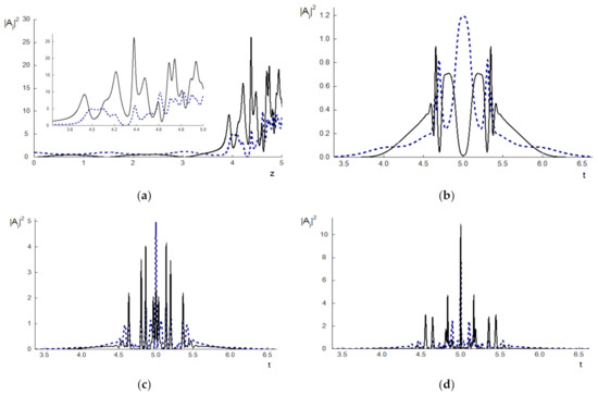
Figure 1.
The intensity evolution at the pulse center () (a) and pulse shapes in sections z = 3 (b), 4 (c), 5 (d) for the BW (dashed line) and TH (solid line) wave.
This occurs due to a very complicated interaction of two waves. It is illustrated by Figure 1 in which the pulse shapes for the first harmonic (FH) wave and third harmonic (TH) wave, as well as the intensity evolution at the pulse centers, are depicted during computation using both FDSs with small mesh steps . Because the computer simulation results obtained using both FDSs coincide, we depict only the results computed using the CFDS-I3. The mutual focusing of the pulses occurring after a certain propagation distance is observed in Figure 1a. As a result, a strong nonlinear regime of the pulse interaction is realized, and the pulse intensities grow significantly and achieve a value that is approximately 27 times greater than the incident pulse intensity.
The pulse shape evolution is depicted in Figure 1b–d. We see in Section 4 and Section 5 of a medium (Figure 1c,d) a formation of high intensity sub-pulses which may propagate separately, and the duration of these sub-pulses is about ten times shorter than the incident pulse duration. In section z = 5, one can see the sub-pulses with soliton-like shape (Figure 1d) with their centers at time moments (and two other ones localized symmetrically), respectively. Therefore, the influence of the second-order derivative on time increases about hundred times and that is why the role of the Hamiltonian is enhanced.
However, if the mesh step on z-coordinate is increased, for example, until , the difference between the computer simulation results obtained using two FDSs appears when the pulse propagation distance exceeds 4.5. Therefore, the main difference between two FDSs is observed when a mutual self-compression of the pulses appears. Up to the section of a medium, the pulse shapes computed using both FDSs coincide and are the same as they are depicted in Figure 1b,c. However, after this distance, we see a very clear difference between the problem solutions computed using CFDS-I3 and CFDS-I1 (see Figure 2a,b). Analysis of the pulse shapes depicted in Figure 2c,d confirms this conclusion; one can see changing certain sub-pulse shapes in section of a medium. Nevertheless, sub-pulses with soliton-like shapes are the same at computation using both FDSs. This means that the pulse carrier frequencies do not contain a time-dependent modulation. Another very important conclusion following from numerical modeling is that the CFDS-I3 allows us to use a significantly larger mesh step on z-coordinate (at least ten times greater) in comparison with the corresponding value for the CFDS-I1 to achieve the adequate computer simulation results.
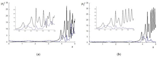
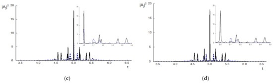
Figure 2.
The intensity evolution at the pulse center () of the BW (dashed line) and TH (solid line) wave (a,b) and their pulse shapes in section z = 5 (c,d) computed using the CFDS-I3 (a,c) and CFDS-I1 (b,d).
5.2. The Invariant Approximation Order for the Split-Step Methods
The approximation order of the invariants when using the Strang methods is illustrated by Table 3 for the parameters: and fixed mesh step on time coordinate. One can see that both invariants preserve the second order of approximation to the spatial coordinate in accordance with the theoretical estimations (Theorem 3), and the SSMRK preserves the energy’s invariant even better than the ISSM. However, if the SOD coefficients are increased ten times (until the value , then the invariant deviations increase, and their approximation order decreases up to the first order (Table 4) when using the ISSM for computer simulation. Moreover, both numerical methods become sensitive to the mesh step on the longitudinal coordinate, and for the mesh step one can see the Hamiltonian deviation dramatically increasing, which results in the problem solution distortion. This is a result of increasing influence of the SOD coefficients because they define changing the phases of the pulses at mesh fixed steps. If a change of the pulse phase increases for two neighboring mesh steps on a spatial coordinate, then their product can be greater than , and therefore, less than two mesh nodes will belong to the period of the phase changing. As a result, the solution becomes wrong, and the problem Hamiltonian deviates from its initial value. Because using of SSMRK requires introducing additional mesh step at solving the stage of the pulse’s nonlinear propagation, computation of the pulse phase is more accurate, and more than three mesh nodes on the spatial coordinate will belong to the period of the phase change compared to using ISSM. That is why the SSMRK demonstrates partly better results in comparison with computation based on ISSM.
Table 3.
Influence of the spatial step on the energy invariant deviation and the Hamiltonian deviation when using the ISSM and the SSMRK for computation. The upper row corresponds to the local invariant deviation, the low row–to the integral deviation of the invariants.
Table 4.
Influence of the spatial step on the first invariant and the Hamiltonian deviation when using the ISSM and the SSMRK for computation. The upper row corresponds to the local invariant deviation, the low row–to the integral deviation of the invariants.
Thus, one can see that the approximation order of the problem invariants correlates with those of FDS only at enough small values of the SOD coefficients.
Although the invariant deviations do not change practically by decreasing the time step from to , the computed solution for these time steps changes and may be wrong. Therefore, the true solution of the problem occurs for (Figure 3a) when using the ISSM or the SSMRK. When increasing the mesh step on the time coordinate, a deviation of the problem solution is not significant until z = 4. (Figure 3b,c). However, change in the problem solution becomes pronounced at . The reason may be the insufficient size of the spectral domain because of the strong broadening of the pulses’ spectra due to the cubic nonlinear response of a medium while the size of the spectral domain decreases by increasing the mesh step on the time coordinate. Therefore, it is necessary to compute at a small enough mesh step in the regime of the waves’ strong nonlinear coupling.
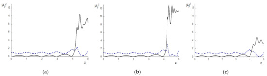
Figure 3.
The intensity evolution at the pulse center for the BW (dashed line) and the TH (solid line) wave computed using the SSMI with mesh steps 0.001 and , respectively.
5.3. Comparison of CFDS with Split-Step Methods
Below, a comparison is made between the computer simulation results obtained using both the CFDS-I3 and the ISSM or the SSMRK for parameters , which correspond to the initial Hamiltonian’s value equal . For definiteness and to achieve a large enough domain in the spectral space, we fix the time mesh step as because such a value is optimal for the problem solution with many sub-pulses. Because the CFDS-I3, ISSM, and SSMRK demonstrate a very small deviation, about of the energy’s invariant, we do not discuss this invariant change. In turn, because the maximal Hamiltonian deviation using CFDS-I3 is less than in dependence of the mesh step h, we also do not show its change along the z-coordinate.
In Figure 4, the pulse intensity evolution at time moment , changing pulse shapes, and the Hamiltonian evolution, are depicted. Their value deviates slightly if a computation is made on the basis of the ISSM, and the worst results demonstrate the SSMRK method (Figure 4c,k), but we clearly see a difference between the solutions computed (Figure 4) when using various FDSs after the coordinate . For example, the TH maximum intensity reaches up to 15 dimensionless units (Figure 4c) at the end of the propagation distance, and this value correlates with a significant deviation of the Hamiltonian (Figure 4k) in this section of a medium. In Figure 4d–f, a difference between the problem solutions computed using the SSMRK and other methods is observed. In section = 4.5 a difference in the solutions, computed using the CFDS-I3 and the ISSM, also appears.
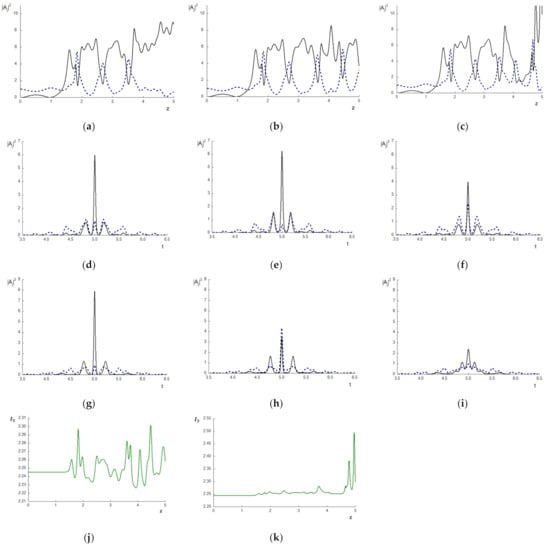
Figure 4.
The intensity evolution at the pulse center (a–c) and pulse shapes in the sections z = 4 (d–f), 4.5 (g–i) for the BW (dashed line) and the TH wave (solid line) and the Hamiltonian deviation computed using the CFDS-I3 (a,d,g), ISSM (b,e,h,j), and SSMRK (c,f,i,k) for , respectively.
To avoid the difference between the problem solutions computed using various FDSs, it is necessary to decrease the mesh step on z-coordinate up to h = 0.002. In this case, change in the Hamiltonian becomes essentially lower in comparison with the previous case, even for the FDSs based on the Strang method (Figure 5b,c). Consequently, the changing of intensities at the pulse centers (Figure 5a–c) and pulse shapes (Figure 5d–f) become closer to each other if the propagation distance is less than 4.5. Nevertheless, beginning from section z = 4.7, the solutions differ, and we see in Figure 5d–f, depicting the pulse shapes in section z = 5, a very pronounced difference between the solutions in time interval from t = 4.55 to t = 5.45, for example.
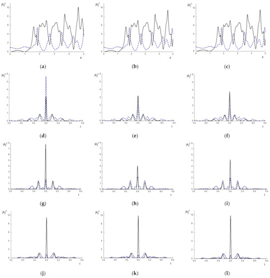
Figure 5.
The intensity evolution at the pulse center (a–c) and pulse shapes in sections z = 5 (d–f), 6 (g–i), 5.5 (j–l), for the BW (dashed line) and the TH wave (solid line) computed using the CFDS-I3 (a,d,g,j), ISSM (b,e,h,k), and SSMRK (c,f,i,l) with , (a–f) and 0.0002 (g–l), respectively.
Further decreasing the mesh step on z-coordinate up to the value h = 2 · , a difference between the FDSs solutions appears only after the section z = 5.6 (Figure 5g–i). The pulse shapes computed using all methods coincide before section z = 5.0 of a medium (Figure 5j–l). The Hamiltonian does not change practically if a computation is based on the ISSM until the propagation distance is about 1.5 dimensionless units: its maximal changing is less than 0.0006. Thereby, if the split-step method is applied for the numerical solution of the THG problem, then with increasing propagation distance, it is necessary to decrease the mesh step on the coordinate along which the laser pulse propagates. This requirement is absent when using the CFDS-I3 for computer simulation.
5.4. Influence of Time Domain on the Computer Simulation Results When Using the Split-Step Method
Clearly, decreasing the time domain leads to enhancing computer simulation efficiency. However, this may lead to losing computation accuracy when using FDSs based on the Strang method. This statement is illustrated by the example depicted in Figure 5j–l for the parameters and for the mesh steps and but for the decreased time domain: . The corresponding computation results are shown in Figure 6. The Hamiltonian does not change if the computation is conducted on the basis of CFDS-I3 (see Figure 6g), and evolution of the pulse center intensity (Figure 6a) coincides with the intensity evolution depicted in Figure 5a, which computed for . It should be stressed that the pulse shapes are also the same as in the previous case. However, using the ISSM and the SSMRK for numerical simulation leads to distortions of the computer simulation results beginning with the section approximately (Figure 6b,c,e,f) despite the small changes on the Hamiltonian (Figure 6h,i). However, in the section the pulses shapes computed using all FDSs coincide with each other (Figure 6j–l). In turn, if the time domain was equal to then the pulses shapes coincided for all FDSs until the section (Figure 5j–l).
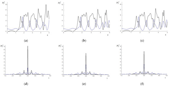
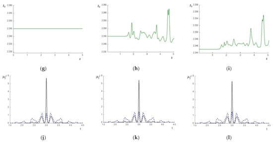
Figure 6.
The intensity evolution at the pulse center (a–c) and pulse shapes in sections z = 4.6 (d–f), 4 (j–l) for the BW (dashed line) and the TH wave (solid line), the Hamiltonian deviation (g–i) computed using the CFDS-I3 (a,d,g,j), ISSM (b,e,h,k), and SSMRK (c,f,i,l), respectively.
Thus, using CFDS-I3 allows us to decrease a domain size on the time coordinate without any losses in computation accuracy. At the same time, the split-step method is very sensitive to this domain size. Hence, when using the split-step method, it is necessary to solve the nonlinear Schrödinger equations in the time domain with a large size to avoid any solution distortion due to the non-zero value of the intensity near the domain boundaries.
5.5. Correlation between the Hamiltonian Deviation and the Intensity Evolution When Using the Strang Method
The disadvantage of the split-step method can appear even for a small value of the SOD coefficients, for example, . We illustrate this with the computer simulation results obtained for and computed in time domain with the mesh step . The first series of computations are made with the mesh step equal 0.02 (see Figure 7a,c,d,c/,d/,k/). Computation based on using the SSMRK does not finish (Figure 7d), and the Hamiltonian changes the sign (see Figure 7d/). The ISSM gives a distorted result (Figure 7c) with large deviation of the Hamiltonian (Figure 7c/), while using CFDS-I3 leads to the numerical solution (Figure 7a) that is very close to the accurate solution and without visible change of the Hamiltonian (Figure 7k/).
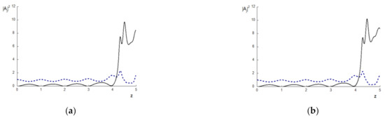

Figure 7.
The intensity evolution at the pulse center (a–f) for the BW (dashed line) and the TH wave (solid line) and the Hamiltonian deviation (c/–f/,i/–k/) computed using the CFDS-I3 (a,b,g,k/), the ISSM (c,e,I,c/,e/,i/), and the SSMRK (d,f,j,d/,f/,j/) for mesh step (a,c,d,c/,d/,k/); (b,e,f,e/,f/); (g,i,j,i/,j/).
By decreasing the mesh step to (Figure 7b,e,f,e/,f/), a difference in the problem solutions obtained using various numerical methods occurs after the section (Figure 7b,e,f). However, this difference is much smaller in comparison with those observed in the previous case. We also observe an essentially small deviation of the Hamiltonian (Figure 7e/,f/) when using the split-step methods. The Hamiltonian does not change at all when conducting computer simulations based on the CFDS-I3. Further decreasing the mesh step h (to ) leads to coinciding solutions obtained using various numerical methods. The Hamiltonian deviation becomes very small (Figure 7i/,j/), and the numerical solution, obtained using the SSMI (Figure 7i) and the SSMRK (Figure 7j), differs from those obtained using the CFDS-I3 (Figure 7g) insignificantly. One can see that Figure 7g does not differ from Figure 7b; there is only the stronger intensity decreasing, and this can be expected because of more accurate computation of the pulse phase change.
Thus, with the appropriate choice of mesh step on the time coordinate, the validity of the numerical solution obtained using the split-step method depends strongly on the Hamiltonian’s preservation. The CFDS-I3 demonstrates accurate results, at least for the spatial mesh step which is six times greater than those using the Strang method.
6. Conclusions
For the set of nonlinear Schrödinger equations describing the THG problem, two CFDSs were developed. Each of the FDSs preserves one of two differential problem’s invariants while another one is preserved with the second order of approximation. These statements were proved theoretically and numerically.
It was shown that the accuracy of the computer simulation results obtained using conservative FDSs depends on which of the problem’s invariants is preserved by the FDS. Therefore, it is preferable if the FDS possess a conservation property on the Hamiltonian because it preserves both a phase relation and intensity shapes between interacting waves.
To demonstrate the efficiency of the developed conservative FDSs, they were compared to a widely used Strang method (split-step method). To improve the stability property of the split-step method, it was modified by using the iteration process on the stage of a solution of the nonlinear ODEs instead of usually used the Runge–Kutta method. Computer simulation results have shown advantages of the CFDSs. In particular, the split-step method is very sensitive to the domain’s size by time coordinate and to the SOD of the pulses. Nevertheless, if the laser pulses’ interaction is not accompanied by a strong self-compression regime, all FDSs give the same results at the corresponding choice of the mesh steps and size of the time domain.
To prove that the conservative FDS gives true results, we compare the numerical solution with the analytical solution developed using the invariants of the problem under consideration. This comparison is shown in Appendix A. A very good coincidence between both solutions is seen. Let us notice that the analytical solution is exact if the SOD coefficients are equal to zero. In the opposite case, this solution is valid on a bounded distance of the laser pulse interaction.
It should be stressed that similar features to those of the FDSs, consisting in their preservation of the Hamiltonian or the energy’s invariant, appear in any problem of optical waves interaction when the energy exchange between interacting waves is present.
Author Contributions
Conceptualization, V.T.; methodology, V.T.; software, V.T.; validation, V.T. and M.L.; investigation, V.T. and M.L.; writing—original draft preparation, V.T.; writing—review and editing, M.L.; visualization, V.T. and M.L.; funding acquisition, M.L. All authors have read and agreed to the published version of the manuscript.
Funding
Loginova M. thanks the Russian Science Foundation (Grant № 19-11-00113) for supporting of this study.
Institutional Review Board Statement
Not applicable.
Informed Consent Statement
Not applicable.
Data Availability Statement
Not applicable.
Conflicts of Interest
The authors declare no conflict of interest.
Appendix A. Comparison of the Analytical Solution with Computer Simulation Results
Below we demonstrate an example of a comparison of one of the analytical solutions developed in [12,14,15,41] with a numerical solution obtained using CFDS-I3. The shape of both incident pulses is a Gaussian function (see (52)) with maximal intensities:
which are equal to
The parameters of the laser pulses interaction are chosen as
For these parameters, an evolution of the TH intensity () at the pulse center () is described by the following formula:
Here, is an elliptic cosine. Parameters are the roots of the characteristic equation, obtained and discussed in our papers. Different solutions corresponding to various modes of the THG were derived in [41]. We emphasize that this solution is accurate, and it was derived in the framework of the long pulse approximation (, j = 1, 3) based on the problem invariants without using the basic wave non-depletion approximation.
The solution (A4) is generalized for the case of the Gaussian shapes of the incident pulses neglecting the influence of the SOD, and in Figure A1, we compare the pulse shape computed using a generalized analytical solution with the results of computer simulation conducted with small mesh steps for the parameters (A2, A3). We see a very good coincidence between these solutions. It means that the developed FDS has high accuracy at an appropriate choice of the mesh steps.

Figure A1.
TH pulse shape in the sections z = 1 (a), 3 (b), 5 (c) computed using CFDS-I3 (solid line) and using analytical formula (red crosses).
Figure A1.
TH pulse shape in the sections z = 1 (a), 3 (b), 5 (c) computed using CFDS-I3 (solid line) and using analytical formula (red crosses).

At the end of Appendix A, we note that the proposed approach for developing the analytical solution on the basis of the problem invariant allows us not only to derive an evolution of the pulse shape but also the phase evolution. This was demonstrated in [42] under the analysis of the SHG problem.
References
- Sandkuijl, D.; Tuer, A.E.; Tokarz, D.; Sipe, J.E.; Barzda, V. Numerical second- and third-harmonic generation microscopy. JOSA B 2013, 30, 382–395. [Google Scholar] [CrossRef]
- Weigelin, B.; Bakker, G.-J.; Friedl, P. Third harmonic generation microscopy of cells and tissue organization. J. Cell Sci. 2016, 129, 245–255. [Google Scholar] [CrossRef] [PubMed]
- Kishida, H.; Hibino, K.; Nakamura, A.; Kato, D.; Abe, J. Third-order nonlinear optical properties of a π-conjugated biradical molecule investigated by third-harmonic generation spectroscopy. Thin Solid Films 2010, 519, 1028–1030. [Google Scholar] [CrossRef]
- Lippitz, M.; van Dijk, A.M.A.; Orrit, M. Third-Harmonic Generation from Single Gold Nanoparticles. Nano Lett. 2005, 5, 799–802. [Google Scholar] [CrossRef] [PubMed]
- Grinblat, G.; Li, Y.; Nielsen, M.P.; Oulton, R.F.; Maier, S.A. Enhanced Third Harmonic Generation in Single Germanium Nanodisks Excited at the Anapole Mode. Nano Lett. 2016, 16, 4635–4640. [Google Scholar] [CrossRef] [PubMed]
- Mikhailov, S.A. Quantum theory of third-harmonic generation in graphene. Phys. Rev. B 2014, 90, 241301. [Google Scholar] [CrossRef]
- Konopsky, V.N.; Alieva, E.V.; Alyatkin, S.Y.; A Melnikov, A.; Chekalin, S.V.; Agranovich, V.M. Phase-matched third-harmonic generation via doubly resonant optical surface modes in 1D photonic crystals. Light Sci. Appl. 2016, 5, e16168. [Google Scholar] [CrossRef] [PubMed][Green Version]
- Markowicz, P.P.; Tiryaki, H.; Pudavar, H.; Prasad, P.N.; Lepeshkin, N.N.; Boyd, R.W. Dramatic Enhancement of Third-Harmonic Generation in Three-Dimensional Photonic Crystals. Phys. Rev. Lett. 2004, 92, 083903. [Google Scholar] [CrossRef]
- Carmon, T.; Vahala, K.J. Visible continuous emission from a silica microphotonic device by third-harmonic generation. Nat. Phys. 2007, 3, 430–435. [Google Scholar] [CrossRef]
- Hajisalem, G.; Nezami, M.S.; Gordon, R. Probing the Quantum Tunneling Limit of Plasmonic Enhancement by Third Harmonic Generation. Nano Lett. 2014, 14, 6651–6654. [Google Scholar] [CrossRef] [PubMed]
- Backus, S.; Peatross, J.; Zeek, Z.; Rundquist, A.; Taft, G.; Murnane, M.M.; Kapteyn, H. 16-fs, 1-μJ ultraviolet pulses generated by third-harmonic conversion in air. Opt. Lett. 1996, 21, 665–667. [Google Scholar] [CrossRef] [PubMed]
- Armstrong, J.A.; Bloembergen, N.; Ducuing, J.; Pershan, P.S. Interactions between Light Waves in a Nonlinear Dielectric. Phys. Rev. 1962, 127, 1918–1939. [Google Scholar] [CrossRef]
- Trofimov, V.A.; Trofimov, V.V.; Yudina, E.A. Theory of THG of high intensive femtosecond laser pulse. Proc. SPIE 2007, 6729, 672935. [Google Scholar] [CrossRef]
- Trofimov, V.A.; Sidorov, P.S.; Kuchik, I.E. Bistable mode of THG for femtosecond laser pulse. Proc. SPIE 2016, 9958, 99580D. [Google Scholar] [CrossRef]
- Trofimov, V.A.; Sidorov, P.S. Influence of SOD on THG for femtosecond laser pulse. Proc. SPIE 2017, 10102, 101021. [Google Scholar] [CrossRef]
- Delfour, M.; Fortin, M.; Payr, G. Finite-difference solutions of a non-linear Schrödinger equation. J. Comput. Phys. 1981, 44, 277–288. [Google Scholar] [CrossRef]
- Sanz-Serna, J.M.; Verwer, J.G. Conservative and Nonconservative Schemes for the Solution of the Nonlinear Schrödinger Equation. IMA J. Numer. Anal. 1986, 6, 25–42. [Google Scholar] [CrossRef]
- Twizell, E.; Bratsos, A.; Newby, J. A finite-difference method for solving the cubic Schrödinger equation. Math. Comput. Simul. 1997, 43, 67–75. [Google Scholar] [CrossRef]
- Wang, H. Numerical studies on the split-step finite difference method for nonlinear Schrödinger equations. Appl. Math. Comput. 2005, 170, 17–35. [Google Scholar] [CrossRef]
- Xie, S.-S.; Li, G.-X.; Yi, S. Compact finite difference schemes with high accuracy for one-dimensional nonlinear Schrödinger equation. Comput. Methods Appl. Mech. Eng. 2009, 198, 1052–1060. [Google Scholar] [CrossRef]
- Wang, T.; Guo, B.; Zhang, L. New conservative difference schemes for a coupled nonlinear Schrödinger system. Appl. Math. Comput. 2010, 217, 1604–1619. [Google Scholar] [CrossRef]
- Wang, D.; Xiao, A.; Yang, W. A linearly implicit conservative difference scheme for the space fractional coupled nonlinear Schrödinger equations. J. Comput. Phys. 2014, 272, 644–655. [Google Scholar] [CrossRef]
- Dehghan, M.; Taleei, A. A compact split-step finite difference method for solving the nonlinear Schrödinger equations with constant and variable coefficients. Comput. Phys. Commun. 2010, 181, 43–51. [Google Scholar] [CrossRef]
- Gao, Z.; Xie, S. Fourth-order alternating direction implicit compact finite difference schemes for two-dimensional Schrödinger equations. Appl. Numer. Math. 2011, 61, 593–614. [Google Scholar] [CrossRef]
- Wang, T.; Guo, B.; Xu, Q. Fourth-order compact and energy conservative difference schemes for the nonlinear Schrödinger equation in two dimensions. J. Comput. Phys. 2013, 243, 382–399. [Google Scholar] [CrossRef]
- Caplan, R.; Carretero-González, R. A two-step high-order compact scheme for the Laplacian operator and its implementation in an explicit method for integrating the nonlinear Schrödinger equation. J. Comput. Appl. Math. 2013, 251, 33–46. [Google Scholar] [CrossRef]
- Moxley, F., III; Chuss, D.T.; Dai, W. A generalized finite-difference time-domain scheme for solving nonlinear Schrödinger equations. Comput. Phys. Commun. 2013, 184, 1834–1841. [Google Scholar] [CrossRef]
- Liu, J. Order of Convergence of Splitting Schemes for Both Deterministic and Stochastic Nonlinear Schrödinger Equations. SIAM J. Numer. Anal. 2013, 51, 1911–1932. [Google Scholar] [CrossRef]
- Caplan, R.; Carretero-González, R. Numerical stability of explicit Runge–Kutta finite-difference schemes for the nonlinear Schrödinger equation. Appl. Numer. Math. 2013, 71, 24–40. [Google Scholar] [CrossRef]
- Hederi, M.; Islas, A.; Reger, K.; Schober, C. Efficiency of exponential time differencing schemes for nonlinear Schrödinger equations. Math. Comput. Simul. 2016, 127, 101–113. [Google Scholar] [CrossRef]
- Lakoba, T.I. Instability of the finite-difference split-step method applied to the generalized nonlinear Schrödinger equation. III. External potential and oscillating pulse solutions. Numer. Methods Partial. Differ. Equ. 2017, 33, 633–650. [Google Scholar] [CrossRef]
- Strang, G. On the Construction and Comparison of Difference Schemes. SIAM J. Numer. Anal. 1968, 5, 506–517. [Google Scholar] [CrossRef]
- Zakharova, I.G.; Karamzin, Y.N.; Trofimov, V.A. About Split-Step Methods for Solving the Nonlinear Optics Problems; Keldysh Institute for Applied Mathematics: Moscow, Russia, 1989; Volume 13, pp. 1–19. [Google Scholar]
- Di Trapani, P.; Caironi, D.; Valiulis, G.; Dubietis, A.; Danielius, R.; Piskarskas, A. Observation of Temporal Solitons in Second-Harmonic Generation with Tilted Pulses. Phys. Rev. Lett. 1998, 81, 570–573. [Google Scholar] [CrossRef]
- Trofimov, V.A.; Matusevich, O.V. Comparison of Efficiency of Various Difference Schemes for the Problem of SHG in Media with Quadratic and Cubic Nonlinear Response. In Proceedings of the Fourth International Conference, Finite Difference Methods: Theory and Application, Lozenetz, Bulgaria, 18–23 June 2007; pp. 320–325. [Google Scholar]
- LeVenque, R.J. Finite Difference Methods for Ordinary and Partial Differential Equations; SIAM: Philadelphia, PA, USA, 2007. [Google Scholar]
- Shampine, L. Conservation laws and the numerical solution of ODEs. Comput. Math. Appl. 1986, 12B, 1287–1296. [Google Scholar] [CrossRef]
- Barletti, L.; Brugnano, L.; Caccia, G.F.; Iavernaro, F. Energy-conserving methods for the nonlinear Schrödinger equation. Appl. Math. Comput. 2018, 318, 3–18. [Google Scholar] [CrossRef]
- Boyd, R.W. Nonlinear Optics, 3rd ed.; Academic Press: Cambridge, MA, USA, 2008. [Google Scholar]
- Li, C. Nonlinear Optics; Springer: Berlin/Heidelberg, Germany, 2017. [Google Scholar]
- Trofimov, V.A.; Sidorov, P.S. Analysis of THG modes for femtosecond laser pulse. Proc. SPIE 2017, 10228, 102280B. [Google Scholar] [CrossRef]
- Trofimov, V.A.; Kharitonov, D.M.; Fedotov, M.V. Theory of SHG in a medium with combined nonlinear response. JOSA B 2018, 35, 3069–3087. [Google Scholar] [CrossRef]


Publisher’s Note: MDPI stays neutral with regard to jurisdictional claims in published maps and institutional affiliations. |
© 2021 by the authors. Licensee MDPI, Basel, Switzerland. This article is an open access article distributed under the terms and conditions of the Creative Commons Attribution (CC BY) license (https://creativecommons.org/licenses/by/4.0/).