Performance of a Novel Chaotic Firefly Algorithm with Enhanced Exploration for Tackling Global Optimization Problems: Application for Dropout Regularization

Abstract

Swarm intelligence techniques have been created to respond to theoretical and practical global optimization problems. This paper puts forward an enhanced version of the firefly algorithm that corrects the acknowledged drawbacks of the original method, by an explicit exploration mechanism and a chaotic local search strategy. The resulting augmented approach was theoretically tested on two sets of bound-constrained benchmark functions from the CEC suites and practically validated for automatically selecting the optimal dropout rate for the regularization of deep neural networks. Despite their successful applications in a wide spectrum of different fields, one important problem that deep learning algorithms face is overfitting. The traditional way of preventing overfitting is to apply regularization; the first option in this sense is the choice of an adequate value for the dropout parameter. In order to demonstrate its ability in finding an optimal dropout rate, the boosted version of the firefly algorithm has been validated for the deep learning subfield of convolutional neural networks, with respect to five standard benchmark datasets for image processing: MNIST, Fashion-MNIST, Semeion, USPS and CIFAR-10. The performance of the proposed approach in both types of experiments was compared with other recent state-of-the-art methods. To prove that there are significant improvements in results, statistical tests were conducted. Based on the experimental data, it can be concluded that the proposed algorithm clearly outperforms other approaches.

1. Introduction

Swarm intelligence is popular in the field of optimization. However, as the “no free lunch” theorem infers, no single algorithm is universally the best performing algorithm for all problems. Hence, many techniques inspired by the behaviors of living organisms have been developed and applied for theoretical and practical tasks, including function optimization, parameter and method calibration, and efficiency improvement in industrial scenarios.

The current paper introduces a modified version of the firefly algorithm (FA) and verifies its boosted abilities on global optimization tasks. The FA [1] is a well-known SI algorithm that has shown great promise in the field of optimization based on metaheuristics. The proposed method is theoretically tested on two bound-constrained benchmark sets: (i) with chosen functions from the CEC test suite, with 10, 30, and 100 dimensions; and (ii) with challenging CEC2017 bound-constrained problems. Finally, from the practical perspective, the proposed approach was applied for dropout approximation.

The FA was chosen as the base for augmentation as it has been successfully validated for various NP-hard challenges in the machine learning domain [2,3,4], including the dropout estimation problem [5], and it shows great potential. However, it was also established that the basic FA suffers from some deficiencies and it is assumed that its potential can be further improved by performing modification of its original version. Furthermore, the performance of SI algorithms for a dropout regularization challenge was not investigated enough.

The field of machine learning suffers from overfitting, otherwise known as high variance, and it appears along every model. The question is not if the model will overfit, but rather about how much it will overfit. While the variance is high, the value of the bias is at its lowest, which is the deviation from the predicted value. The trade-off between these two parameters has to be made without any of the two gravitating towards their extreme values. The difficulty arises when the data set is modest in size, which leaves less space for adjusting. Convolutional neural networks (CNN) tackle this problem with the method of dropout regularization, which has proven to be efficient in solving these types of scenarios. In this process, random neurons are selected for exclusion from the layers during the training phase. This results in a higher bias, which translates to a more precise model, but the key is moderation, because of the previously mentioned trade-off.

Dropout is estimated manually and tested by trial and error, which is unsustainable in cases where the model is complex. Dropout estimation by swarm intelligence algorithms can help solve this problem. Algorithms that are considered swarm-like heuristics have had success with solving NP-hard problems, including dropout estimation. CNN and SI algorithms are metaheuristics; they are influenced by concepts from nature. CNNs take inspiration from the human visual cortex and SI algorithms take inspiration from animals that move, live, and gather resources in large groups, called swarms. Recent research shows that the hybrid solutions between machine learning and swarm intelligence provide better results [6,7,8]. These types of hybrid solutions are more optimized and scalable.

The observed results indicate improvement from the original algorithm on the tested CEC benchmarks and better results with the CNN. As mentioned before, overfitting is unavoidable. One of the solutions is regularization—this is the process of preventing overfitting. The complexity of the model is controlled through regularization techniques. Models with a larger number of features result in a large number of weights, considering that every feature is assigned a certain weight. The loss function returns the difference between the predicted and the actual label. Different techniques of regularization exist, among which, the most popular are L1, L2, and dropout regularization. The dropout method carries significant importance because of the high accuracy of the model, while the loss is very low. The other techniques perform well in established scenarios; however, there is a certain lack of evidence of stable performance.

The main objective behind the approach proposed in this study is to further improve the FA, from the theoretical side, increase the classification performance of CNNs, and avoid the overfitting issue by proper establishment of the dropout regularization parameter, from a practical scope. Furthermore, since the potential of metaheuristics for this type of challenge was not investigated enough, 10 other well-known swarm intelligence approaches were also implemented and tested for this problem. The contribution of this research is three-fold:

• A novel modified FA algorithm was implemented by specifically targeting the known flaws of the basic implementation of the FA approach;
• The devised algorithm was later utilized to help establish the proper dropout value and enhancing the CNN accuracy;
• Other well-known swarm intelligence metaheuristics for CNN dropout regularization challenge were further investigated.

The rest of the paper is organized in the following manner. Section 2 describes the fundamental technologies used (swarm intelligence and CNN). Section 3 introduces the modified version of the algorithm, as well as the original one. Section 4 provides the results of the experiments. Section 5 deals with the optimization of the dropout parameter, and the final observations are given in Section 6.

2. Preliminaries and Related Works

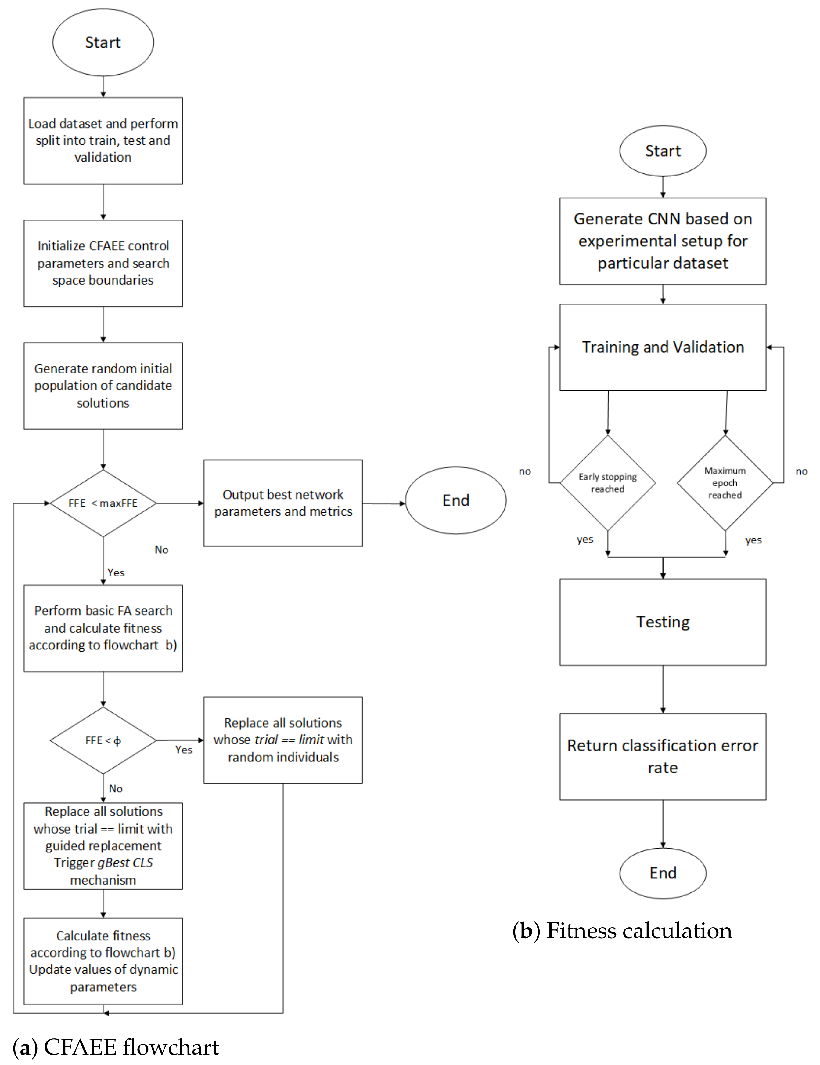
Improving an existing solution by modifying an algorithm, i.e., via another metaheuristic approach, yields good results in this field. Metaheuristic solutions are stochastic, and for an algorithm to be categorized as metaheuristic, it must be inspired by a certain process in the nature. These processes come from group animal behaviors, in which animals work towards a common goal, unachievable by solely working alone. This type of behavior exhibits group intelligence. The intellectual potential of a single unit of a species is not very high. On the contrary, while in large groups, even simple organisms perform complex tasks successfully. The solutions inspired by these kinds of animals are metaheuristic and belong to the field of swarm intelligence, which has proven successful in solving NP-hard problems. This has been exploited in algorithm hybridization for improving machine learning algorithms; this type of combination is referred to as learnheuristics.

In this work, dropout regularization improvement was achieved by the previously mentioned methods. Swarm intelligence is a metaheuristic field that adapts animal behavior, specifically in animals that move in swarms, in regard to algorithms used in the field of artificial intelligence [9,10]. The field of SI has a wide application because it efficient in solving NP-hard problems. SI methods have been frequently used to address different optimization tasks, both theoretical [11] and from various practical fields, including wireless sensor networks (WSNs) [12,13,14,15], task scheduling in the cloud, and edge computing [16,17]. Recently, one of the most important fields of interest has been the hybrid approach with SI and machine learning. The number of publications in this domain increased drastically in recent years; some of the most prominent works include hyperparameter optimization [3,18,19], feature selection problems [2], time series prediction tasks, e.g., estimation of COVID-19 cases [6,20], and neural network training [21,22].

Hybridization of these algorithms yields the most benefits. With this approach, it is possible to significantly improve convergence times. SI algorithms apply a stochastic approach in the search of global optima, making them heavily reliant on the number of iterations. This process is divided into two phases, exploration and exploitation, similar to the training and testing phases in machine learning. In exploration, the focus is on exploring the local search area, while the latter phase is global. These phases must be balanced out, again, similar to the training and testing phases in machine learning. The SI goal is not to achieve the best solution, but rather to quickly provide a sub-optimal one. The search for the best solution can be greatly enhanced by adding evolutionary principles to the algorithm. The evolutionary algorithms implement a mechanism that transfers the knowledge from the previous population to the next one. This is achieved through mutation, crossover, and selection. Mutation can be translated into the algorithm, keeping a unit from the previous generation, but with the modification of the value it carries. Crossover is the combination of two neurons, and selection is the process of selecting the best units. This is a different approach compared to the random generation of a hive population. Evolution-based swarms are prone to provide faster convergence compared to the classic population-based swarm algorithms, but are less sensitive in terms of finding local optima, as they can get more easily stuck in them.

The SI method proposed in this paper regards an augmentation of the FA algorithm. The improved version was tested on several benchmark theoretical functions, before it is applied to dropout optimization in CNN.

Humans are highly visual creatures and rely heavily on this sense. This translates to limitations of input that can be used for machine learning. While the field yielded tremendous results in big data and prediction-based insights, most of the ideas that employ AI required visual input. For the majority of adopters, which are non-professional individuals, the only contact with AI is by using certain software that manipulates the visual input. While these tasks are trivial, in regard to changing one’s appearance, the true importance of this adoption lies in the previously mentioned nature of our species. Humans are not computational beings. Therefore, the human species does not process any of the information absorbed by labeling, tagging, and placing into tables. This creates a limitation for the accurate representation of the information obtained in the computational form. It is inefficient and too complex of a process for an individual to translate the obtained information from a photograph into words (in a way that a program can process them). As a result, CNNs have been widely applied because they excel in these types of tasks, including speech recognition, natural language processing, and computer vision. These models must be ‘modeled’, such as the human nervous system [23,24,25]. The most recent applications include facial recognition [26,27,28,29], document analysis [30,31,32], image classification tasks in medicine as support for diagnostic processing and faster illness detection [33,34,35], analysis of climate change and extreme weather prediction [36,37], and many others. The metaheuristic approach in CNN comes from the animal visual cortex. The visual cortex is built from layers that receive, segment, and integrate visual input. The output of each layer is the input for the next layer. During this process, the data get cleaner as they get deeper. This means that data are simplified, making it easier to process further, while retaining all of the important features. An example of this behavior is edge forming on the first layer, the set of edges and corners on the second layer, sets of corners and contours and parts of objects on the third layer and, finally, the full object on the last layer. The convolution layer, pooling layer, and the fully connected layer, in that order, represent the anatomy of a CNN.

Firstly, the convolution layers apply the corresponding operations, which filter the data. It is important to emphasize that the filters are always smaller in size from the input. Widely used sizes are 3 × 3, 5 × 5, and 7 × 7. The convolution operation of the input vector is:

$$z_{i,j,k}^{\left[l\right]}=w_k^{\left[l\right]}{x}_{i,j}^{\left[l\right]}+b_k^{\left[l\right]}$$

(1)

The symbols from the equation bear the following meaning: $z_{i,j,k}^{\left[l\right]}$ denotes the output feature value of the k-th feature map at location $i,j$, the input is x at the location $i,j$, w represents filters, and bias is b.

The activation operation is:

$$g_{i,j,k}^{\left[l\right]}=g\left(z_{i,j,k}^{\left[l\right]}\right),$$

(2)

where $g(·)$ denotes the non-linear function exploiting the output.

There are two types of pooling layers: global and local. The most widely used method is the max and average pooling.

The resolution is reduced through the pooling function:

$$y_{i,j,k}^{\left[l\right]}=pooling\left(g_{i,j,k}^{\left[l\right]}\right)$$

(3)

Classification is performed by the fully connected layers. The softmax layer performs multi-classification. In the case of binary classification, the logistic layer is used.

As stated in Section 1, several techniques are used to avoid the overfitting issue; one of them is dropout regularization. This research focuses on optimizing the dropout probability ($dp$); hence, the dropout regularization is explained in the following paragraphs.

In light of the proposed CNN model, the dropout technique can be considered a new CNN layer. With this in mind, r denotes the activation or dropout of M nodes in the observed layer. Every variable $r_j$ is assigned the value of 1 with probability $1-p$, independently. If the observed $r_j$ contains the value 1, then that unit remains in the network, and if not, then that particular unit is removed from the network with all of its connections.

The probability p is unconstrained from other cells in the network, and it is obtained from the Bernoulli distribution, described with the Equation (4).

$$r_j\sim Bernoulli\left(p\right),\forall j=1,2,\cdots ,M$$

(4)

With this in mind, it is possible to denote the outputs vector of a layer L with $y^{\left(L\right)}$ during the network training. After applying the dropout, the new outputs vector ${\tilde{y}}^{\left(L\right)}$ can be defined by Equation (5):

$${\tilde{y}}^{\left(L\right)}=r{y}^{\left(L\right)}$$

(5)

At the end, during the network testing, the weight matrix W is required to be scaled by ratio p for averaging all $2^M$ possible networks that have dropped out. This step summarizes the main contributions of the regularization method, because it is needed to test a single network, as shown in Equation (6).

$$W_{test}^{\left(L\right)}=p{W}^{\left(L\right)}$$

(6)

where $W^{\left(L\right)}$ denotes the weight matrix at layer L.

3. Proposed Method

This beginning section introduces the basic implementation of the FA metaheuristics, followed by the discussion about the known and observed flaws and drawbacks of the original version. At the end, a detailed description of the proposed modified method that is devised to specifically overcome these flaws of the original algorithm is provided.

3.1. The Original Firefly Algorithm

The FA metaheuristics, introduced by Yang [1], is motivated by flashing and social characteristics of fireflies. Since, in the ‘real-world’, the natural system is relatively complex and sophisticated, the FA models it by using several approximation rules [1].

Brightness and attractiveness of fireflies are used for modeling fitness functions; attractiveness, in most typical FA implementations, depend on the brightness, which is in turn determined by the objective function value. In the case of minimization problems, it is formulated as [1]:

$$I\left(x\right)=\left\{\begin{array}{cc}{\displaystyle \frac{1}{f\left(x\right)}}\hfill & ,\mathrm{if}f\left(x\right)>0\hfill \\ 1+\mid f\left(x\right)\mid \hfill & ,\mathrm{otherwise}\hfill \end{array}\right.$$

(7)

where $I\left(x\right)$ represents attractiveness and $f\left(x\right)$ denotes the value of objective function at location x.

Light intensity; hence, the attractiveness of the individual decreases, as the distance from the light source increases [1]:

$$I\left(r\right)={\displaystyle \frac{I_0}{1+\gamma r^2}}$$

(8)

where $I\left(r\right)$ represents light intensity at the distance r, while $I_0$ stands for the light intensity at the source. Furthermore, for modeling real natural systems, where the light is partially absorbed by its surroundings, the FA makes use of the $\gamma$ parameter, which represents the light absorption coefficient. In most FA versions, the combined effect of the inverse square law for distance and the $\gamma$ coefficient is approximated with the following Gaussian form [1]:

$$I\left(r\right)=I_0·e^{-\gamma r^2}$$

(9)

Moreover, each firefly individual utilizes attractiveness $\beta$, which is directly proportional to the light intensity of a given firefly and also depends on the distance, as shown in Equation (10).   

$$\beta \left(r\right)={\beta }_0·e^{-\gamma r^2}$$

(10)

where parameter ${\beta }_0$ designates attractiveness at distance $r=0$. It should be noted that, in practice, Equation (10) is often replaced by Equation (11) [1]:

$$\beta \left(r\right)={\displaystyle \frac{{\beta }_0}{1+\gamma r^2}}$$

(11)

Based on the above, the basic FA search equation for a random individual i, which moves in iteration $t+1$ to a new location $x_i$ towards individual j with greater fitness, is given as [1]:

$$x_i^{t+1}=x_i^t+{\beta }_0·e^{-\gamma r_{i,j}^2}(x_j^t-x_i^t)+{\alpha }^t(\kappa -0.5)$$

(12)

where $\alpha$ stands for the randomization parameter, the random number drawn from Gaussian or a uniform distribution is denoted as $\kappa$, and $r_{i,j}$ represents the distance between two observed fireflies i and j. Typical values that establish satisfying results for most problems for ${\beta }_0$ and $\alpha$ are 1 and $[0,1]$, respectively.

The $r_{i,j}$ is the Cartesian distance, which is calculated by using Equation (13).

$$r_{i,j}=\left|\right|x_i-x_j\left|\right|=\sqrt{\sum _{k=1}^D{(x_{i,k}-x_{j,k})}^2}$$

(13)

where D marks the number specific problem parameters.

3.2. Motivation for Improvements

Notwithstanding the outstanding performance of original FA for many benchmarks [38] and practical challenges [39], findings of previous studies suggest that the basic FA shows some deficiencies in terms of insufficient exploration and inadequate intensification-diversification balance [40,41,42]. The lack of diversification is particularly emphasized in early iterations, when, in some runs, the algorithm is not able to converge to optimal search space regions, and ultimately worse mean values are obtained. In such scenarios, a basic FA search procedure (Equation (12)), which primarily conducts exploitation, is not able to guide the search towards optimum domains. Conversely, when in the initialization phase, random solutions are generated by chance in the optimal or near-optimal regions, the FA manages to obtain satisfying results.

Further, by analyzing a fundamental FA search equation (Equation (12)), it can be observed that it does not encompass an explicit exploration procedure. To address this issue, some FA implementations utilize the dynamic randomization parameter $\alpha$, where this parameter is gradually decreased from its initial value ${\alpha }_0$ towards the predefined threshold ${\alpha }_{min}$, as shown in Equation (14). In this way, at the beginning of a run, exploration is more emphasized, while in later iterations, the balance between intensification and diversification moves towards exploitation [43]. However, based on the extensive empirical simulations, it is deduced that the application of dynamic $\alpha$ is not enough to enhance FA exploration abilities and the proposed mechanism only slightly eliminates this issue.

$${\alpha }^{t+1}={\alpha }^t·\left(1-{\displaystyle \frac{t}{T}}\right),$$

(14)

where t and $t+1$ denote current and next iteration, respectively, while the T is the maximum iteration number in one run of an algorithm.

It is also worth noting that the previous studies show that FA exploitation abilities are efficient in tackling various kinds of tasks, and FA is known as metaheuristic, with robust exploitation capabilities [40,41,42].

3.3. Novel FA Metaheuristics

A novel FA approach proposed in this study addresses issues of the basic FA by assimilating the following procedures:

• Explicit exploration mechanism based on the solution’s exhaustiveness;
• gBest chaotic local search (CLS) strategy.

No matter what the outstanding exploitation capabilities of the original FA are, by using the CLS mechanism, intensification can further improve, as shown in the empirical section of this manuscript.

Motivated by proposed enhancements, a novel FA is named chaotic FA with enhanced exploration (CFAEE).

3.3.1. Explicit Exploration Mechanism

The goal of the explicit exploration procedure is to assure that the algorithm converges to the optimum part of the search space in early iteration, while in late phases of execution, it facilitates exploration around the parameter boundaries of the current best individual $x^{*}$. To incorporate this behavior, each solution is modeled by using additional attributes $trial$, which is incremented every time when the solution cannot be improved by the basic FA search (Equation (12)). When the $trial$ parameter for a particular solution reaches a predetermined $limit$ value, the individual is replaced with the random solution drawn from within the boundaries of the search space by utilizing the same procedure as in the initialization phase:

$$x_{i,j}=l_j+(u_j-l_j)·rand,$$

(15)

where $x_{i,j}$ represents j-th component of i-th individual, $u_j$ and $l_j$ denote upper and lower search boundaries of the j-th parameter, and $rand$ is a uniformly distributed random number from the interval $[0,1]$.

The solution, which $trial$ exceeds the $limit$, is said to become exhaustive. This idea, as well as terminology, was adapted from the well-known ABC metaheuristics [44], which are known to have efficient exploration mechanisms [45].

Replacement of the exhausted solution, with a pseudo-random individual, stirs up search performances in early iterations, when the algorithm does not identify proper parts of the search region. However, in later iterations, following the reasonable assumption that the optimal region has been found, this kind of replacement wastes function evaluations. For that reason, in later iterations, the random replacement procedure is changed with the guided replacement mechanism around the lower and upper parameter values of all solutions in the population:

$$x_{i,j}=P{l}_j+(P{u}_j-P{l}_j)·rand,$$

(16)

where $P{l}_j$ and $P{u}_j$ represent the lowest and highest values of the j-th component from the entire population P.

3.3.2. The gBest CLS Strategy

The chaos as random phenomenon exists in non-linear and deterministic systems and is highly responsive to its initial condition [46]. From the mathematical perspective, chaotic search is more efficient than the ergodic one [47], because a vast number of sequences can be generated by only tweaking its initial values.

Notwithstanding that, in modern literature, many chaotic maps exist, after conducting empirical experiments, it was concluded that, in case of the proposed novel FA, the logistic map obtains the most promising results. We should note that the logistic map has been utilized in many swarm intelligence approaches [48,49,50].

The logistic map that the proposed method utilizes executes in K steps and it is defined as:

$${\sigma }_{i,j}^{k+1}=\mu {\sigma }_{i,j}^k(1-{\sigma }_{i,j}),k=1,2,\dots K,$$

(17)

where ${\sigma }_{i,j}^k$ and ${\sigma }_{i,j}^{k+1}$ represent chaotic variable for j-th component of the i-th solution in steps k and $k+1$, respectively, and $\mu$ is control variable. The ${\sigma }_{i,j}\ne 0.25,0.5$ and $0.75$, ${\sigma }_{i,j}\in (0,1)$ and $\mu$ is set to 4, since this value was previously determined empirically [50].

The proposed method incorporates the global best (gBest) CLS strategy because the chaotic search is performed around the $x^{*}$ solution. In each step k, new $x^{*}$, denoted as ${x\prime }^{*}$, is generated with the Equations (18) and (19), which are applied for to component j of $x^{*}$:

$$x_j^{\prime *}=(1-\lambda )x_j^{*}+\lambda S_j$$

(18)

$$S_j=l_j+{\sigma }_j^k(u_j-l_j)$$

(19)

where ${\sigma }_j^k$ is determined by Equation (17) and $\lambda$ is the dynamic shrinkage parameter that depends on the current fitness function evaluation ($FFE$) and on the maximum number of fitness function evaluations ($maxFFE$) in the run:

$$\lambda =\frac{maxFFE-FFE+1}{maxFFE}$$

(20)

By using dynamic $\lambda$, better exploitation–exploration equilibrium around the $x^{*}$ is established. In earlier phases of the execution, a wider search radius around the $x^{*}$ was explored, while in the later phases, a fine-tuned exploitation was performed. The $FFE$ and $maxFFE$ can be replaced with t and T when the maximum number of iterations is taken as the termination condition.

In this way, by using the CLS strategy, $x^{*}$ is (attempted to be) improved in K steps, and if the $x^{\prime *}$ obtains better fitness than the $x^{*}$, the CLS procedure is terminated, and the $x^{*}$ is replaced with $x^{\prime *}$. However, if in K steps the $x^{*}$ could not be improved, it is retained in the population.

3.3.3. Chaotic FA with Enhanced Exploration Pseudo-Code

In order to efficiently incorporate the exploration mechanism and gBest CLS strategy in the original FA, a few things should be considered. First, as already suggested in Section 3.3.1, in the early phases of the execution, the random replacement mechanism should be conducted, while in latter phases, the guided one would generate better results. Second, the gBest CLS strategy, in early iterations, would not generate significant improvements because the $x^{*}$ likely still did not converge to the optimum region, and it would just waste $FFEs$.

To control the above mentioned behavior, the additional control parameter $\psi$ is included in the following way: if $t<\psi$, the exhausted solutions from the population are replaced with the random ones (Equation (15)) and the gBest CLS will not be executed; if $t\ge \psi$, the guided replacement mechanism will be executed (Equation (16)) and the gBest CLS will be triggered.

Moreover, to fine-tune, the basic FA search proposed method utilizes dynamic $\alpha$, according to Equation (14).

Taking all of the above, the pseudo-code of the proposed CFAEE is summarized in Algorithm 1.

Algorithm 1 The CFAEE pseudo-code

Initialize main metaheuristics control parameters N and T

Initialize search space parameters D, $u_j$ and $l_j$

Initialize CFAEE control parameters $\gamma$, ${\beta }_0$, ${\alpha }_0$, ${\alpha }_{min}$, K and $\varphi$

Generate initial random population $P_{init}=\left\{x_{i,j}\right\},i=1,2,3\dots ,N;j=1,2,,\dots D$ using Equation (15) in the search space

while$t<T$do

for $i=1$ to N do

for $z=1$ to i do

if $I_z<I_i$ then

Move solution z in the direction of individual i in D dimensions (Equation (12))

Attractiveness changes with distance r as exp[$-\gamma r$] (Equation (10))

Evaluate new solution, replace the worse individual with better one and update intensity of light (fitness)

end if

end for

end for

if $t<\varphi$ then

Replace all solutions for which $trial=limit$ with random ones using Equation (15)

else

Replace all solutions for which $trial=limit$ with guided replacement using Equation (16)

for $k=1$ to K do

Perform gBest CLS around the $x^{*}$ using Equations (17)–(19) and generate $x^{\prime }*$

Retain better solution between $x^{*}$ and $x^{\prime *}$

end for

end if

Update $\alpha$ and $\lambda$ according to Equations (14) and (20), respectively

end while

Return the best individual $x_{*}$ from the population

Post-process results and perform visualization

3.3.4. The CFAEE Complexity and Drawbacks

The number of FFEs can be taken as a metric to determine the complexity of the swarm intelligence algorithm because the most computationally expensive part is the objective evaluation [38]. The basic FA evaluates objective functions in the initialization and in the solution updating phases. While updating solutions, according to the Equation (12), the FA employs one main loop for T iterations and two inner loops going through N solutions [38].

Thus, including the initialization phase, the worst case complexity of basic FA metaheuristics is $O\left(N\right)+O(N^2·T)$. However, if N is relatively large, it is possible to use one inner loop by ranking the attractiveness or brightness of all fireflies using sorting algorithms, and in this case, complexity is $O\left(N\right)+O(N·T·log\left(N\right))$ [38].

The complexity of the proposed CFAEE is higher than the original FA due to the application of the explicit exploration mechanism and gBest CLS strategy. In the worst case scenario, if the $limit=0$, all solutions will be replaced in every iteration, and the gBest CLS strategy will be triggered throughout the whole run if $\varphi =0$. Assuming that the value of K is set to 4, then the worst case CFAEE complexity is given as: $O\left(N\right)+O(T·N^2)+O(T·N)+O(4·T)$. However, in practice, the complexity is much better because of $limit$ and $\psi$ control parameter adjustments.

Drawbacks of the proposed CFAEE over the original version involve utilization of additional control parameters $limit$ and $\psi$. However, conducting empirical simulations, values of these parameters can be relatively easy determined. Moreover, the employment of these two parameters is justified because the CFAEE exhibits substantial performance improvements over the original FA for benchmark challenges and for the dropout regularization challenge from the machine learning domain, as shown in Section 4 and Section 5.

4. Bound-Constrained Benchmark Simulations

The proposed novel FA was first rigorously tested on a set of standard bound-constrained benchmarks that encompass functions from the well-known Congress on Evolutionary Computation (CEC) benchmark suite and other notable instances. The first benchmark set consists of 18 carefully chosen complex uni-modal, multi-modal, and two-dimensional functions, with the goal of determining convergence speed and exploration ability of the proposed method. Comparative analysis was performed with another state-of-the-art FA version. The purpose of the second benchmark set, which includes challenging CEC2017 unconstrained functions, is to measure the robustness and efficiency of the proposed CFAEE over other the state-of-the-art swarm intelligence metaheuristics.

4.1. Experimental Setup

Due to the stochastic nature of metaheuristics, the only way to determine proper control parameter values is by performing a “trial and error” approach on a wider set of theoretical problems, such as extensively utilized bound-constrained benchmarks. Afterwards, the results for a set of independent runs are averaged, and control parameters that obtain the best mean performances are utilized in further experiments. This is usual practice for establishing proper control parameter values for novel and improved implementations of existing metaheuristics approaches [1,51,52,53].

Following the above-mentioned firmly established practice, the optimal (or near-optimal) CFAEE control parameter setup was determined by conducting extensive simulations on classical unconstrained benchmarks. The goal was to find control parameter values that would, on average, for all test instances, accomplish satisfying results.

The CFAEE control parameter values that were utilized in both bound-constrained simulations are shown in

Table 1. Setup of CFAEE control parameters.

Parameter and Notation	Value
Number of solution N	20 (benchmark1), 30 (benchmark2)
Maximum number of $FFE$ ($maxFFE$)	160,000 (benchmark1), 15,030 (benchmark2)
Absorption coefficient $\gamma$	1.0
Attractiveness at $r=0$ ${\beta }_0$	1.0
Randomization (step) $\alpha$	changes according to Equation (14)
Initial value of step ${\alpha }_0$	0.5
Minimum value of step ${\alpha }_{min}$	0.1
Solutions’ exhaustiveness $limit$	$maxFFE/N·2$
CLS strategy step number K	4
CLS strategy $\lambda$	changes according to Equation (20)
Parameter $\varphi$	$maxFFE/2$

. Since the CFAEE may utilize different number of $FFE$ in each run, the $maxFFE$ is used as termination criteria instead of T. Expressions for calculating values of $limit$ and $\varphi$ parameters are also determined empirically.

Both bound-constrained experiments were executed in 50 independent runs and all methods included in the comparative analysis were implemented for the purpose of this research. All algorithms were implemented in Python by using core (built-in), as well as specific data science and machine learning Python libraries: NumPy, SciPy, pandas, scikit-learn, pyplot, and seaborn.

All experiments were conducted on Intel^® CoreTM i7-8700K CPU and 32 GB of RAM running, using a Windows 10 × 64-bit operating system computer platform.

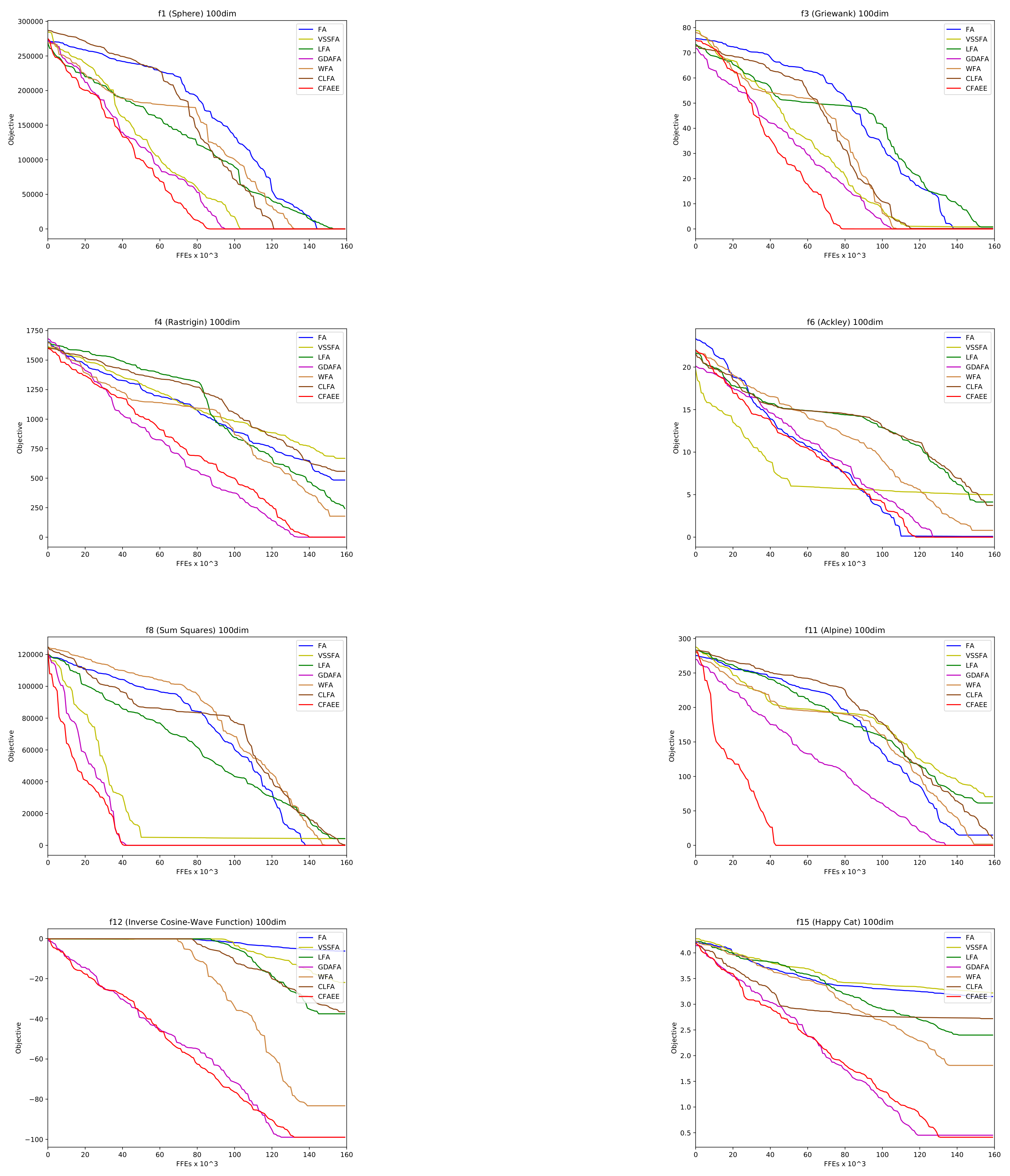
4.2. Benchmark Problem Set 1

The goal of the first bound-constrained simulation was to validate convergence speed and exploration ability of the proposed method against other state-of-the-art FA approaches. The same ‘opponent’ algorithms and the same test beds as in [54] are included in the analysis.

Table 2. Function details for benchmarks problem set I.

ID	Name	Search Range	Formulation	Optimum
f1	Sphere	${[-100,100]}^D$	min $f\left(x\right)={\sum }_{i=1}^D{x}_i^2$	0
f2	Moved Axis Function	${[-5.12,5.12]}^D$	min $f\left(x\right)={\sum }_{i=2}^{D}5i{x}_i^2$	0
f3	Griewank	${[-100,100]}^D$	min $f\left(x\right)={\sum }_{i=1}^D\frac{x_i^2}{4000}-{\prod }_{i=1}^{D}cos\left(\frac{x_i}{\sqrt{i}}\right)+1$	0
f4	Rastrigin	${[-5.12,5.12]}^D$	min $f\left(x\right)=10n+{\sum }_{i=1}^D[x_i^2-10cos\left(2\pi x_i\right)]$	0
f5	The Schwefel’s Problem 1.2	${[-100,100]}^D$	min $f\left(x\right)={\sum }_{i=1}^D{\sum }_{j=1}^i{x}_j^2$	0
f6	Ackley	${[-32,32]}^D$	min $f\left(x\right)=-a\times exp(-b\sqrt{\frac{1}{n}{\sum }_{i=1}^n{x}_i^2})-exp(\frac{1}{D}{\sum }_{i=1}^{n}cos\left(c{x}_i\right))+a+exp\left(1\right)$, where $a=20,b=0.2$	0
f7	Powell Sum	${[-1,1]}^D$	min $f\left(x\right)={\sum }_{i=1}^D{\left|x_i\right|}^{i+1}$	0
f8	Sum Squares	${[-10,10]}^D$	min $f\left(x\right)={\sum }_{i=1}^{D}i{x}_i^2$	0
f9	Schwefel 2.22	${[-100,100]}^D$	min $f\left(x\right)={\sum }_{i=1}^D|x_i|+{\prod }_{i=1}^n\left|x_i\right|$	0
f10	Powell Singular	${[-4,5]}^D$	min $f\left(x\right)={\sum }_{i=1}^{D/4}[{(x_{4i-3}+10x_{4i-2})}^2+5{(x_{4i-1}-x_{xi})}^2+{(x_{4i-2}-2x_{4i-1})}^4+10{(x_{4i-3}+x_{4i})}^4]$	0
f11	Alpine	${[-10,10]}^D$	min $f\left(x\right)={\sum }_{i=1}^D\left|x_{i}sin\left(x_i+0.1x_i\right)\right|$	0
f12	Inverse Cosine-Wave Function	${[-100,100]}^D$	min $f\left(x\right)={\sum }_{i=1}^{D-1}(exp(-\frac{x_i^2+x_{i+1}^2+0.5x_i{x}_{i+1}}{8})\times cos\left(4\sqrt{x_i^2+x_{i+1}^2+0.5x_i{x}_{i+1}}\right))$	−D+1
f13	Pathological	${[-100,100]}^D$	min $f\left(x\right)={\sum }_{i=1}^{D-1}{\left(0.5+\frac{{sin}^2\left(\sqrt{100x_i^2+x_{i+1}^2}\right)-0.5}{1+0.001{\left(x_i^2-2x_i{x}_{i+1}+x_{i+1}^2\right)}^2}\right)}^2$	0
f14	Discus	${[-100,100]}^D$	min $f\left(x\right)={10}^6{x}_1^2+{\sum }_{i=1}^D{x}_i^2$	0
f15	Happy Cat	${[-2,2]}^D$	min $f\left(x\right)={\left[{(\left|\left|x_i^2\right|\right|-D)}^2\right]}^{\alpha }+{\displaystyle \frac{1}{D}}(0.5\left|\left|x_i^2\right|\right|+{\sum }_{i=1}^D{x}_i)+0.5$, where $\alpha ={\displaystyle \frac{1}{4}}$	0
f16	Drop-Wave Function	${[-5.2,5.2]}^D$	min $f\left(x\right)=-{\displaystyle \frac{1+cos\left(12\sqrt{x_1^2+x_2^2}\right)}{(0.5(x_1^2+x_2^2)+2)}}$	−1
f17	Schaffer 2	${[-100,100]}^D$	min $f\left(x\right)=0.5+{\displaystyle \frac{{sin}^2{(x_1^2-x_2^2)}^2-0.5}{1+0.001{(x_1^2+x_2^2)}^2}}$	0
f18	Camel Function-Three Hump	${[-5,5]}^D$	min $f\left(x\right)=2x_1^2-1.05x_1^4+{\displaystyle \frac{x_1^6}{6}}+x_1{x}_2+x_2^2$	0

provides details of carefully chosen unconstrained benchmark instances that were used in experiments. Tests $f1,f3,f4,f5,f6,f7,f14$, and $f15$ are provided by the benchmark suite of the CEC. Remaining functions represent basic tests used to evaluate the convergence of algorithms and quality of solutions. In addition, all test functions possess diverse characteristics. Firstly, the complex uni-modal functions that only have the global optimum are $f1,f2,f5,f7,f8,f12$, and $f14$. These functions are used for the purpose of convergence speed testing. Secondly, the multi-modal functions that have a variety of local optima are $f3,f4,f6,f9,f10,f11,f13$, and $f15$ and their purpose is to test the ability of an algorithm to pull through from local solutions, which is the measure of exploration ability. Finally, the highly complex two-dimensional functions with various local minima are also included $f16,f17$, and $f18$.

State-of-the-art FA versions that were included in he comparative analysis are the following: dynamic adaptive weight firefly algorithm (WFA) [55], chaotic FA based on logistic map (CLFA) [56], Levy flights FA (LFA) [57], variable step size firefly algorithm for numerical optimization (VSSFA) [58], and the dynamically adaptive firefly algorithm with global orientation (GDAFA) [54].

In [54], all of the above-mentioned FA approaches were tested with $N=20$ and $T=1000$ per run, which, in the worst case, yielded a total of 400,040 $FFE$ (please refer to Section 3.3.4). However, empirically, it was determined that not all $N·N$ evaluations were executed in each iteration and the best approximation would be $FFE/2.5$, which is around 160,000. Thus, in this research, experiments provided in [54] were recreated with $FFE=$ 160,000 for all methods in order to establish fair comparative analysis because the proposed CFAEE utilizes more $FFE$ in each iteration than other opponent methods. Basic control parameter setups for all FA versions are the same, as shown in Table 1; for their other specific parameters, please refer to [54].

It should be noted that, for all methods, except for the basic FA, similar results as in [54] were obtained. In the conducted experiments, basic FA with dynamic parameter $alpha$ (Equation (14)) was used, and much better results than reported in [54] were obtained. Authors in [54] implemented a static FA approach, and other proposed improved FA methods established better performance.

All simulations were conducted with 10, 30, and 100 dimensions ($D=[10,30,100]$) for benchmark function instances from $f1$ to $f15$ and comparative analysis results were summarized in

Table 3. Comparative analysis among CFAEE, original FA, and five other FA implementations for benchmarks with 10 dimensions.

Function	Algorithm	Best Value	Worst Value	Mean Value	Function	Algorithm	Best Value	Worst Value	Mean Value
$f_1\left(x\right)$	FA VSSFA LFA GDAFA WFA CLFA CFAEE	0 0 0 0 $5.019\times {10}^{-3}$ 0 0	$2.91\times {10}^{-5}$ 0 0.531452 0 0.116521 0 0	$6.07\times {10}^{-7}$ 0 0.151967 0 0.067858 0 0	$f_9\left(x\right)$	FA VSSFA LFA GDAFA WFA CLFA CFAEE	0 0 0 0 $5.18\times {10}^{-2}$ 0 0	$1.00\times {10}^{-3}$ 0 0.735625 0 0.79956 0 0	$2.00\times {10}^{-5}$ 0 0.327158 0 0.431151 0 0
$f_2\left(x\right)$	FA VSSFA LFA GDAFA WFA CLFA CFAEE	0 0 0 0 $1.64\times {10}^{-3}$ 0 0	$5.15\times {10}^{-7}$ 0 5.74765 0 4.005821 0 0	$1.06\times {10}^{-8}$ 0 1.32645 0 1.003456 0 0	$f_{10}\left(x\right)$	FA VSSFA LFA GDAFA WFA CLFA CFAEE	$1.25\times {10}^{-6}$ 0 0 0 $4.82\times {10}^{-2}$ 0 0	$3.29\times {10}^{-6}$ 0 14.95923 0 9.18410 0 0	$2.28\times {10}^{-6}$ 0 2.736795 0 3.381069 0 0
$f_3\left(x\right)$	FA VSSFA LFA GDAFA WFA CLFA CFAEE	$9.60\times {10}^{-4}$ 0 0 0 $8.63\times {10}^{-5}$ 0 0	$9.60\times {10}^{-4}$ 0 $5.32\times {10}^{-2}$ 0 $1.65\times {10}^{-2}$ 0 0	$9.60\times {10}^{-4}$ 0 $7.45\times {10}^{-3}$ 0 $7.32\times {10}^{-3}$ 0 0	$f_{11}\left(x\right)$	FA VSSFA LFA GDAFA WFA CLFA CFAEE	0 0 0 0 $1.96\times {10}^{-2}$ 0 0	$3.02\times {10}^{-7}$ 0 0.451043 0 0.224532 0 0	$6.30\times {10}^{-9}$ 0 0.145892 0 0.131779 0 0
$f_4\left(x\right)$	FA VSSFA LFA GDAFA WFA CLFA CFAEE	5.969720 1.12073 0 0 2.537912 2.142703 0	5.969720 16.96541 4.352192 0 22.243001 27.135292 0	5.969720 7.962931 2.160021 0 10.984211 11.528380 0	$f_{12}\left(x\right)$	FA VSSFA LFA GDAFA WFA CLFA CFAEE	−3.007700 −7.416352 −9 −9 −9 −7.982860 −9	−3.007700 −6.100051 −8.154811 −9 −6.738521 −5.318621 −9	−3.007740 −6.821470 −8.837092 −9 −7.182860 −6.730021 −9
$f_5\left(x\right)$	FA VSSFA LFA GDAFA WFA CLFA CFAEE	0 0 0 0 $1.15\times {10}^{-2}$ 0 0	$1.35\times {10}^{-5}$ 0 1.216521 0 0.668310 0 0	$2.81\times {10}^{-7}$ 0 0.371654 0 0.315237 0 0	$f_{13}\left(x\right)$	FA VSSFA LFA GDAFA WFA CLFA CFAEE	0.502000 $1.35\times {10}^{-3}$ 0 0 $8.63\times {10}^{-4}$ $1.64\times {10}^{-4}$ 0	0.502000 $2.51\times {10}^{-2}$ $8.69\times {10}^{-3}$ 0 $8.29\times {10}^{-2}$ $2.52\times {10}^{-2}$ 0	0.502000 $7.95\times {10}^{-3}$ $1.72\times {10}^{-3}$ 0 $1.82\times {10}^{-2}$ $8.44\times {10}^{-3}$ 0
$f_6\left(x\right)$	FA VSSFA LFA GDAFA WFA CLFA CFAEE	$1.46\times {10}^{-14}$ $8.88\times {10}^{-16}$ $8.88\times {10}^{-16}$ $8.88\times {10}^{-16}$ $7.63\times {10}^{-2}$ $8.88\times {10}^{-16}$ $8.88\times {10}^{-16}$	$1.90\times {10}^{-3}$ $8.88\times {10}^{-16}$ 1.156728 $8.88\times {10}^{-16}$ 1.197652 $8.88\times {10}^{-16}$ $8.88\times {10}^{-16}$	$3.8\times {10}^{-5}$ $8.88\times {10}^{-16}$ 0.363197 $8.88\times {10}^{-16}$ 0.569403 $8.88\times {10}^{-16}$ $8.88\times {10}^{-16}$	$f_{14}\left(x\right)$	FA VSSFA LFA GDAFA WFA CLFA CFAEE	643.025312 0 0 0 $2.63\times {10}^{-3}$ 0 0	697.974622 0 0.634750 0 0.177280 0 0	644.124100 0 $6.42\times {10}^{-2}$ 0 $7.34\times {10}^{-2}$ 0 0
$f_7\left(x\right)$	FA VSSFA LFA GDAFA WFA CLFA CFAEE	$1.61\times {10}^{-7}$ 0 0 0 $4.65\times {10}^{-13}$ 0 0	$1.83\times {10}^{-7}$ 0 $1.05\times {10}^{-2}$ 0 $2.55\times {10}^{-3}$ 0 0	$1.62\times {10}^{-7}$ 0 $1.52\times {10}^{-3}$ 0 $8.15\times {10}^{-9}$ 0 0	$f_{15}\left(x\right)$	FA VSSFA LFA GDAFA WFA CLFA CFAEE	1.753800 0 0 0 0.622315 0 0	1.753800 0.432198 0.453921 0 0.978813 0.635291 0	1.753800 $4.62\times {10}^{-2}$ 0.168663 0 0.860170 0.160825 0
$f_8\left(x\right)$	FA VSSFA LFA GDAFA WFA CLFA CFAEE	0 0 0 0 $1.69\times {10}^{-2}$ 0 0	$1.08\times {10}^{-6}$ 0 1.413521 0 0.727350 0 0	$2.24\times {10}^{-8}$ 0 0.237733 0 0.355913 0 0

,

Table 4. Comparative analysis among CFAEE, original FA, and five other FA implementations for benchmarks with 30 dimensions.

Function	Algorithm	Best Value	Worst Value	Mean Value	Function	Algorithm	Best Value	Worst Value	Mean Value
$f_1\left(x\right)$	FA VSSFA LFA GDAFA WFA CLFA CFAEE	0 13.62752 9.542603 0 0.143725 $8.69\times {10}^{-2}$ 0	$3.30\times {10}^{-4}$ 20.168334 17.455290 $3.71\times {10}^{-4}$ 0.329325 0.335712 6.25$\times {10}^{-6}$	$8.47\times {10}^{-6}$ 17.05007 14.08179 $1.61\times {10}^{-5}$ 0.237264 0.194190 1.41$\times {10}^{-6}$	$f_9\left(x\right)$	FA VSSFA LFA GDAFA WFA CLFA CFAEE	0 15.668320 7.896512 0 0.759455 0.663490 0	$7.15\times {10}^{-3}$ 18.532451 13.652705 4.84$\times {10}^{-3}$ 1.652710 2.0693 $5.17\times {10}^{-3}$	$7.43\times {10}^{-4}$ 17.168332 11.634482 $6.22\times {10}^{-4}$ 1.444582 1.444582 6.09$\times {10}^{-4}$
$f_2\left(x\right)$	FA VSSFA LFA GDAFA WFA CLFA CFAEE	0 952.735293 495.234239 0 9.0823 8.458129 0	$5.73\times {10}^{-4}$ 1292.759201 932.959210 $5.31\times {10}^{-4}$ 27.288553 35.736666 3.52 $\times {10}^{-5}$	$1.19\times {10}^{-5}$ 1151.53123 831.976505 $4.63\times {10}^{-5}$ 15.382611 19.345189 4.52 $\times {10}^{-6}$	$f_{10}\left(x\right)$	FA VSSFA LFA GDAFA WFA CLFA CFAEE	$5.52\times {10}^{-4}$ 740.533299 1297.755023 0 3.545252 5.3022 0	$1.48\times {10}^{-3}$ 4352.542059 3675.442951 $1.53\times {10}^{-2}$ 33.82541 28.982541 1.13 $\times {10}^{-3}$	$8.79\times {10}^{-4}$ 2953.135592 2626.920051 $1.30\times {10}^{-3}$ 23.710392 17.315642 4.44 $\times {10}^{-4}$
$f_3\left(x\right)$	FA VSSFA LFA GDAFA WFA CLFA CFAEE	$9.86\times {10}^{-3}$ 0.453243 0.331970 0 $5.43\times {10}^{-3}$ $5.45\times {10}^{-3}$ 0	$9.87\times {10}^{-3}$ 0.573032 0.511440 1.84 $\times {10}^{-5}$ $3.65\times {10}^{-2}$ $1.76\times {10}^{-2}$ $5.79\times {10}^{-5}$	$9.86\times {10}^{-3}$ 0.516954 0.446482 $4.65\times {10}^{-6}$ $1.23\times {10}^{-2}$ $9.97\times {10}^{-3}$ 2.33 $\times {10}^{-6}$	$f_{11}\left(x\right)$	FA VSSFA LFA GDAFA WFA CLFA CFAEE	$1.66\times {10}^{-2}$ 13.115620 6.718345 0 0.245052 0.133675 0	$1.86\times {10}^{-2}$ 16.344592 13.539203 $3.34\times {10}^{-3}$ 0.731462 0.475093 8.54 $\times {10}^{-4}$	$1.66\times {10}^{-2}$ 14.957239 10.529380 $4.69\times {10}^{-4}$ 0.417792 0.312399 1.03 $\times {10}^{-4}$
$f_4\left(x\right)$	FA VSSFA LFA GDAFA WFA CLFA CFAEE	53.728352 91.368000 26.842502 0 10.562432 48.503233 0	53.728352 145.032962 47.888361 0.293775 70.887502 118.455291 0.163325	53.728352 131.851977 37.948270 $6.33\times {10}^{-2}$ 52.398675 89.757932 2.31 $\times {10}^{-2}$	$f_{12}\left(x\right)$	FA VSSFA LFA GDAFA WFA CLFA CFAEE	−2.745302 −14.281512 −19.773059 −29 −27.135292 −19.932444 −29	−2.738143 −10.236442 −14.387294 −28.981153 −23.462555 −13.572562 −28.975432	−2.741055 −12.601748 −17.381692 −28.995732 −25.463931 −16.488942 −28.997240
$f_5\left(x\right)$	FA VSSFA LFA GDAFA WFA CLFA CFAEE	0 188.932905 175.893044 0 1.363823 1.167251 0	$8.10\times {10}^{-4}$ 249.742592 248.643292 $1.33\times {10}^{-4}$ 5.757921 7.374155 7.35 $\times {10}^{-5}$	$1.69\times {10}^{-5}$ 229.451399 218.334752 $1.51\times {10}^{-5}$ 3.464743 3.888032 5.65 $\times {10}^{-6}$	$f_{13}\left(x\right)$	FA VSSFA LFA GDAFA WFA CLFA CFAEE	4.821110 $4.86\times {10}^{-2}$ $5.92\times {10}^{-2}$ $2.48\times {10}^{-32}$ $4.28\times {10}^{-2}$ $3.85\times {10}^{-2}$ 4.34 $\times {10}^{-34}$	4.854329 $9.37\times {10}^{-2}$ 0.135155 $8.75\times {10}^{-6}$ 0.131320 $9.92\times {10}^{-2}$ 3.13 $\times {10}^{-6}$	4.831800 $7.24\times {10}^{-2}$ $8.63\times {10}^{-2}$ $1.08\times {10}^{-6}$ $7.60\times {10}^{-1}$ $6.16\times {10}^{-2}$ 7.09 $\times {10}^{-7}$
$f_6\left(x\right)$	FA VSSFA LFA GDAFA WFA CLFA CFAEE	$3.95\times {10}^{-12}$ 4.340823 3.011800 $8.88\times {10}^{-16}$ 0.433632 0.447690 $8.88\times {10}^{-16}$	$4.08\times {10}^{-1}$ 4.530665 3.725154 $2.51\times {10}^{-2}$ 0.855143 2.853752 1.05 $\times {10}^{-2}$	$8.17\times {10}^{-2}$ 4.493832 3.383214 2.87 $\times {10}^{-3}$ 0.688177 1.1317517 $4.65\times {10}^{-3}$	$f_{14}\left(x\right)$	FA VSSFA LFA GDAFA WFA CLFA CFAEE	$1.26\times {10}^{+4}$ 16.331 12.645 0 $3.54\times {10}^{-2}$ 0.10623 0	$1.29\times {10}^{+4}$ 22.498 20.226 $3.01\times {10}^{-4}$ 0.50956 0.42646 1.15 $\times {10}^{-4}$	$1.26\times {10}^{+4}$ 19.8985 16.6886 $4.50\times {10}^{-5}$ 0.261277 0.244281 2.29 $\times {10}^{-5}$
$f_7\left(x\right)$	FA VSSFA LFA GDAFA WFA CLFA CFAEE	6.16e-05 123.295565 21.954921 0 4.57E-11 3.52e-08 0	6.18e-05 1158.432456 4319.824940 3.17e-38 1.38e-03 9.83e-03 4.91 $\times {10}^{-39}$	$6.17\times {10}^{-5}$ 541.478399 1345.324915 $7.91\times {10}^{-40}$ $9.67\times {10}^{-5}$ $1.25\times {10}^{-5}$ 3.12 $\times {10}^{-41}$	$f_{15}\left(x\right)$	FA VSSFA LFA GDAFA WFA CLFA CFAEE	2.3302 2.262251 0.723335 0 1.175841 1.307425 0	2.3302 2.348725 1.466781 0.637052 1.371513 1.743721 0.592563	2.3302 2.305134 1.060788 9.92$\times {10}^{-2}$ 1.294690 1.524977 $9.98\times {10}^{-2}$
$f_8\left(x\right)$	FA VSSFA LFA GDAFA WFA CLFA CFAEE	0 152.832522 103.285692 0 1.534341 1.561 0	3.17e-04 275.964302 214.365219 $5.93\times {10}^{-4}$ 4.781903 5.175238 2.22 $\times {10}^{-4}$	$8.12\times {10}^{-5}$ 235.952315 173.448925 $4.62\times {10}^{-5}$ 3.255770 3.270697 9.29 $\times {10}^{-6}$

and

Table 5. Comparative analysis among CFAEE, original FA, and five other FA implementations for benchmarks with 100 dimensions.

Function	Algorithm	Best Value	Worst Value	Mean Value	Function	Algorithm	Best Value	Worst Value	Mean Value
$f_1\left(x\right)$	FA VSSFA LFA GDAFA WFA CLFA CFAEE	0 86.457552 84.743562 0 0.776975 6.0074 0	$5.08\times {10}^{-3}$ 94.965352 101.550299 $5.33\times {10}^{-3}$ 1.343821 9.086351 3.35 $\times {10}^{-3}$	$3.06\times {10}^{-4}$ 91.851742 95.331892 $1.67\times {10}^{-3}$ 1.123621 7.397248 2.12 $\times {10}^{-4}$	$f_9\left(x\right)$	FA VSSFA LFA GDAFA WFA CLFA CFAEE	7.270000 75.261423 61.271532 0 4.667233 19.453222 0	7.345340 79.183492 69.287492 0.282980 7.217744 29.786432 0.253300	7.272472 76.237822 65.957970 6.75 $\times {10}^{-2}$ 5.953690 24.393170 $8.03\times {10}^{-2}$
$f_2\left(x\right)$	FA VSSFA LFA GDAFA WFA CLFA CFAEE	$6.45\times {10}^{-2}$ 20,155.732954 20,134.629495 0 183.584823 1439.319025 0	0.861329 23,097.569290 23,511.452949 2.732509 326.044592 2483.724942 0.525656	0.296353 21,435.685432 22,061.730052 0.263728 246.343291 1955.372492 0.255429	$f_{10}\left(x\right)$	FA VSSFA LFA GDAFA WFA CLFA CFAEE	0.113550 24,876.459003 24,626.324592 0 95.657422 688.787853 0	0.754291 29,942.359392 33,338.728942 0.769235 143.859235 1431.750099 0.621509	0.212700 27,295.176529 29,210.135929 $6.36\times {10}^{-2}$ 116.538544 1058.681232 5.31 $\times {10}^{-2}$
$f_3\left(x\right)$	FA VSSFA LFA GDAFA WFA CLFA CFAEE	$1.11\times {10}^{-1}$ 0.783852 0.746025 0 $1.16\times {10}^{-2}$ 0.167315 0	0.354451 0.850443 0.837694 1.25 $\times {10}^{-4}$ $2.35\times {10}^{-2}$ 0.186983 $1.38\times {10}^{-4}$	0.195824 0.811365 0.799866 $3.55\times {10}^{-5}$ $9.38\times {10}^{-5}$ 0.166489 2.13$\times {10}^{-5}$	$f_{11}\left(x\right)$	FA VSSFA LFA GDAFA WFA CLFA CFAEE	14.775500 68.413502 58.357421 0 1.295332 7.397541 0	15.145392 73.163592 65.772001 2.27 $\times {10}^{-2}$ 2.282315 11.648522 $2.48\times {10}^{-2}$	14.950132 70.657632 61.465342 $4.53\times {10}^{-3}$ 1.686960 9.200357 3.02 $\times {10}^{-3}$
$f_4\left(x\right)$	FA VSSFA LFA GDAFA WFA CLFA CFAEE	436.882200 638.513205 223.195002 0 113.543829 476.735252 0	551.395213 706.697495 263.465402 1.653533 213.352932 613.530234 1.293298	484.606492 668.543402 243.792502 0.589842 178.416452 558.464329 0.539520	$f_{12}\left(x\right)$	FA VSSFA LFA GDAFA WFA CLFA CFAEE	-4.445052 −23.0423521 −44.356992 −99 −87.920501 −40.345210 −99	−8.728848 −19.167452 −34.123586 −98.835492 −79.465202 −27.446501 −98.872555	−6.178500 −21.911352 −37.588482 −98.947900 −83.891430 −36.452653 −98.962902
$f_5\left(x\right)$	FA VSSFA LFA GDAFA WFA CLFA CFAEE	2428.940492 4012.652903 3888.542030 0 33.682005 293.459724 0	2592.352049 4633.727049 4683.634029 0.418092 72.436405 518.965567 0.435304	2433.183441 4315.743555 4365.895902 $8.25\times {10}^{-2}$ 53.696570 385.652334 4.67 $\times {10}^{-2}$	$f_{13}\left(x\right)$	FA VSSFA LFA GDAFA WFA CLFA CFAEE	20.651103 0.162015 0.147652 $1.53\times {10}^{-32}$ 0.142465 0.117900 3.65 $\times {10}^{-33}$	20.770492 0.187683 0.191543 $8.75\times {10}^{-5}$ 0.186110 0.169890 3.33 $\times {10}^{-5}$	20.659945 0.169435 0.175026 $1.30\times {10}^{-5}$ 0.163519 0.154551 9.66 $\times {10}^{-6}$
$f_6\left(x\right)$	FA VSSFA LFA GDAFA WFA CLFA CFAEE	$1.11\times {10}^{-13}$ 4.924155 4.140800 $8.88\times {10}^{-16}$ 0.635644 3.269543 $8.88\times {10}^{-16}$	$9.43\times {10}^{-2}$ 5.442632 4.543301 $3.59\times {10}^{-2}$ 1.108742 4.236500 2.75 $\times {10}^{-2}$	$1.89\times {10}^{-2}$ 5.032945 4.412393 1.03 $\times {10}^{-2}$ 0.845798 3.732709 $1.26\times {10}^{-2}$	$f_{14}\left(x\right)$	FA VSSFA LFA GDAFA WFA CLFA CFAEE	$1.70\times {10}^{+5}$ 93.691550 95.931103 0 0.880193 8.075650 0	$1.72\times {10}^{+5}$ 105.629021 109.031902 $3.28\times {10}^{-3}$ 1.358399 14.832029 2.83 $\times {10}^{-3}$	$1.71\times {10}^{+5}$ 100.355603 103.562900 6.53 $\times {10}^{-4}$ 1.099707 11.357613 $6.85\times {10}^{-4}$
$f_7\left(x\right)$	FA VSSFA LFA GDAFA WFA CLFA CFAEE	$7.30\times {10}^{-4}$ $1.31\times {10}^{+15}$ $1.75\times {10}^{+18}$ 0 $3.17\times {10}^{-9}$ 21978.054329 0	$7.38\times {10}^{-4}$ $6.49\times {10}^{+17}$ $1.41\times {10}^{+22}$ $2.35\times {10}^{-31}$ $5.56\times {10}^{-3}$ $2.27\times {10}^{+11}$ 3.45 $\times {10}^{-32}$	$7.33\times {10}^{-4}$ $1.38\times {10}^{+16}$ $1.76\times {10}^{+21}$ $5.16\times {10}^{-33}$ $4.27\times {10}^{-4}$ $9.45\times {10}^{+9}$ 6.65$\times {10}^{-34}$	$f_{15}\left(x\right)$	FA VSSFA LFA GDAFA WFA CLFA CFAEE	3.158222 3.186900 2.271819 0 1.756300 2.569432 0	3.158339 3.256833 2.492549 0.786523 1.896942 2.835301 0.725431	3.158275 3.225253 2.405293 0.451663 1.8131570 2.704312 0.417902
$f_8\left(x\right)$	FA VSSFA LFA GDAFA WFA CLFA CFAEE	0.185455 $4.10\times {10}^{+3}$ $3.54\times {10}^{+3}$ 0 36.945444 293.842003 0	0.499821 $4.63\times {10}^{+3}$ $4.79\times {10}^{+3}$ 0.567650 73.345992 486.513050 0.475325	0.289011 $4.23\times {10}^{+3}$ $4.25\times {10}^{+3}$ $5.12\times {10}^{-2}$ 53.455374 375.451515 3.19 $\times {10}^{-2}$

, respectively. Comparative analysis results with two-dimensional functions ($f16-f18$) are provided in

Table 6. Comparative analysis among CFAEE, original FA, and five other FA implementations for benchmarks with 2 dimensions.

Function	Algorithm	Best Value	Worst Value	Mean Value	Function	Algorithm	Best Value	Worst Value	Mean Value
$f_{16}\left(x\right)$	FA VSSFA LFA GDAFA WFA CLFA CFAEE	−1 −1 −1 −1 −1 −1 −1	−1 −1 −1 −1 −0.95357 −1 −1	−1 −1 −1 −1 −0.997534 −1 −1	$f_{17}\left(x\right)$	FA VSSFA LFA GDAFA WFA CLFA CFAEE	0 0 0 0 0 0 0	$9.65\times {10}^{-13}$ 0 0 0 0 0 0	$1.96\times {10}^{-14}$ 0 0 0 0 0 0
$f_{18}\left(x\right)$	FA VSSFA LFA GDAFA WFA CLFA CFAEE	0 0 0 0 0 0 0	$3.02\times {10}^{-12}$ 0 0 0 $3.52\times {10}^{-5}$ 0 0	$6.29\times {10}^{-14}$ 0 0 0 $1.86\times {10}^{-7}$ 0 0

. In all simulations, best, worst, and mean values averaged over 50 runs are reported. The results in bold and slightly larger font denote the algorithm that showed the best results for that performance metric.

The overall conclusion from all presented results is that the best two methods are proposed—CFAEE and GDAFA. Benchmark instance with $D=10$ are relativity easy for optimization and both methods in each run for all benchmarks obtained optimum results. The most significant performance difference between the original FA and other methods can be observed in the $f14$ test, where the basic version completely failed to converge to the optimum region. On the other hand, the basic FA showed very competitive results for the $f3$ benchmark.

When the benchmarks with $D=30$ were considered, the proposed CFAEE again obtained superior results, leaving the GDAFA approach in second place. The superiority of CFAEE can be seen in $f5$, $f7$, $f8$, and $f13$ benchmarks, where the difference between CFAEE (first), followed by GDAFA (second), and all other observed algorithms, were the most significant. It is also worth noting that the basic FA implementation again performed well, and exhibited competitive performances for the test instances $f1$, $f2$, $f5$, $f9$, and $f10$, where it outperformed several other enhanced FA implementations.

When the most complex benchmarks ($D=100$) are observed, the superiority of the proposed CFAEE can be seen once more. This is most obvious in the test instances $f7$, $f8$, and $f13$, where performance of the CFAEE (first), followed closely by GDAFA (second), were by far the best when compared to all other algorithms, with the most significant difference. The GDAFA, on the other hand, performed very well in test instances $f6$, $f9$, and $f14$, finishing in the first place, in front of the proposed CFAEE. Again, similar as to the $D=10$ and $D=30$ benchmarks, the basic FA implementation performances were very competitive, which can be easily seen for $f1$ and $f6$ benchmarks, where the basic FA performances were close to CFAEE and GDAFA, while leaving other enhanced FA implementations behind.

Finally, for instances with only two dimensions (Table 6), all methods, except FA and WFA, managed to reach optimum in all runs. These complex functions exhibit many local optima and FA and WFA did not show satisfactory exploration ability in all runs. This issue of basic FA is described in Section 3.2.

For making performance differences more clear for the readers—the number of times that each algorithm outperformed the benchmark, as well as each performance indicator, are counted in

Table 7. Summary of benchmark problem set 1 scores.

	FA	VSSFA	LFA	WFA	CLFA	GDAFA	CFAEE
Best 10 dim	0	0	0	0	0	0	0
Mean 10 dim	0	0	0	0	0	0	0
Worst 10 dim	0	0	0	0	0	0	0
Total 10 dim	0	0	0	0	0	0	0
Best 30 dim	0	0	0	0	0	0	1
Mean 30 dim	0	0	0	0	0	2	13
Worst 30 dim	0	0	0	0	0	3	12
Total 30 dim	0	0	0	0	0	5	26
Best 100 dim	0	0	0	0	0	0	1
Mean 100 dim	0	0	0	0	0	3	12
Worst 100 dim	0	0	0	0	0	3	12
Total 100 dim	0	0	0	0	0	6	25
GRAND TOTAL	0	0	0	0	0	11	51

.

Further, to see if there is a statistically significant difference in the results, we applied the Wilcoxon signed rank-test to perform the pair-wise results comparisons between the proposed CFAEE and other improved FA versions, and the original FA algorithm, for 100-dimensional simulations (Table 5). Following the usual practice for determining whether the results came from different distributions, a significance level of $\alpha =0.05$ was taken. It should be noted that the results for $D=10$ and $D=30$ do not exhibit statistically significant differences since low-dimensional and medium-dimensional problems are easy tasks for all methods included in the analysis.

Results of the Wilcoxon signed-rank test are summarized in

Table 8. Statistical comparison of results obtained by CFAEE for 100-dimensional benchmarks with other approaches by the Wilcoxon Signed-Rank Test at $\alpha$ = 0.05.

Function	CFAEE	GDAFA	FA	VSSFA	LFA	WFA	CLFA
f1	$2.12\times {10}^{-4}$	$1.66\times {10}^{-3}$	$3.06\times {10}^{-4}$	$9.16\times {10}^{+1}$	$9.42\times {10}^{+1}$	1.02	7.50
f2	$2.554\times {10}^{-1}$	$2.63\times {10}^{-1}$	$2.96\times {10}^{-1}$	$2.14\times {10}^{+4}$	$2.21\times {10}^{+4}$	$2.47\times {10}^{+2}$	$1.96\times {10}^{+3}$
f3	$2.13\times {10}^{-5}$	$3.50\times {10}^{-5}$	$5.97\times {10}^{-5}$	$8.11\times {10}^{-1}$	$8.00\times {10}^{-1}$	$2.10\times {10}^{-2}$	$1.66\times {10}^{-1}$
f4	$5.395\times {10}^{-1}$	$5.68\times {10}^{-1}$	$4.85\times {10}^{+2}$	$6.69\times {10}^{+2}$	$2.42\times {10}^{+2}$	$1.79\times {10}^{+2}$	$5.56\times {10}^{+2}$
f5	$4.67\times {10}^{-2}$	$8.17\times {10}^{-2}$	$2.43\times {10}^{+3}$	$4.31\times {10}^{+3}$	$4.36\times {10}^{+3}$	$5.06\times {10}^{+1}$	$3.85\times {10}^{+2}$
f6	$1.26\times {10}^{-2}$	$1.08\times {10}^{-2}$	$1.89\times {10}^{-2}$	5.05	4.41	$8.38\times {10}^{-1}$	3.61
f7	$6.65\times {10}^{-34}$	$8.11\times {10}^{-33}$	$7.35\times {10}^{-5}$	$1.29\times {10}^{+17}$	$1.88\times {10}^{+21}$	$1.17\times {10}^{-4}$	$9.54\times {10}^{+9}$
f8	$3.19\times {10}^{-2}$	$5.42\times {10}^{-2}$	$1.89\times {10}^{-1}$	$4.33\times {10}^{+3}$	$4.33\times {10}^{+3}$	$5.15\times {10}^{+1}$	$3.70\times {10}^{+2}$
f9	$8.03\times {10}^{-2}$	$6.85\times {10}^{-2}$	7.27	$7.62\times {10}^{+1}$	$6.58\times {10}^{+1}$	5.95	$2.44\times {10}^{+1}$
f10	$5.31\times {10}^{-2}$	$6.21\times {10}^{-2}$	$2.13\times {10}^{-1}$	$2.73\times {10}^{+4}$	$2.92\times {10}^{+4}$	$1.18\times {10}^{+2}$	$1.06\times {10}^{+3}$
f11	$3.02\times {10}^{-3}$	$4.53\times {10}^{-3}$	$1.48\times {10}^{+1}$	$7.06\times {10}^{+1}$	$6.25\times {10}^{+1}$	1.68	9.20
f12	−$9.89\times {10}^{+1}$	−$9.89\times {10}^{+1}$	−6.18	−$2.09\times {10}^{+1}$	−$3.65\times {10}^{+1}$	−$8.28\times {10}^{+1}$	−$3.64\times {10}^{+1}$
f13	$9.66\times {10}^{-6}$	$1.30\times {10}^{-5}$	$2.07\times {10}^{+1}$	$1.54\times {10}^{-1}$	$1.75\times {10}^{-1}$	$1.56\times {10}^{-1}$	$1.53\times {10}^{-1}$
f14	$6.85\times {10}^{-4}$	$6.23\times {10}^{-4}$	$1.70\times {10}^{+5}$	$9.93\times {10}^{+1}$	$1.02\times {10}^{+2}$	1.10	$1.12\times {10}^{+1}$
f15	$4.17\times {10}^{-1}$	$4.42\times {10}^{-1}$	3.16	3.22	2.41	1.81	2.71
p-value	3.125$\times {10}^{-2}$	4.39$\times {10}^{-2}$	2.13$\times {10}^{-4}$	3.05$\times {10}^{-5}$	3.05$\times {10}^{-5}$	3.05$\times {10}^{-5}$	3.05$\times {10}^{-5}$

. As can be seen from the presented table, the calculated p-value is lesser than the critical level $\alpha =0.05$ in all cases, and it can be concluded that the proposed CFAEE, on average, significantly outperforms all other approaches.

Convergence speed graphs of some functions, averaged over 50 runs for all metaheuristics taken for comparative analysis in Table 5, are shown in Figure 1.

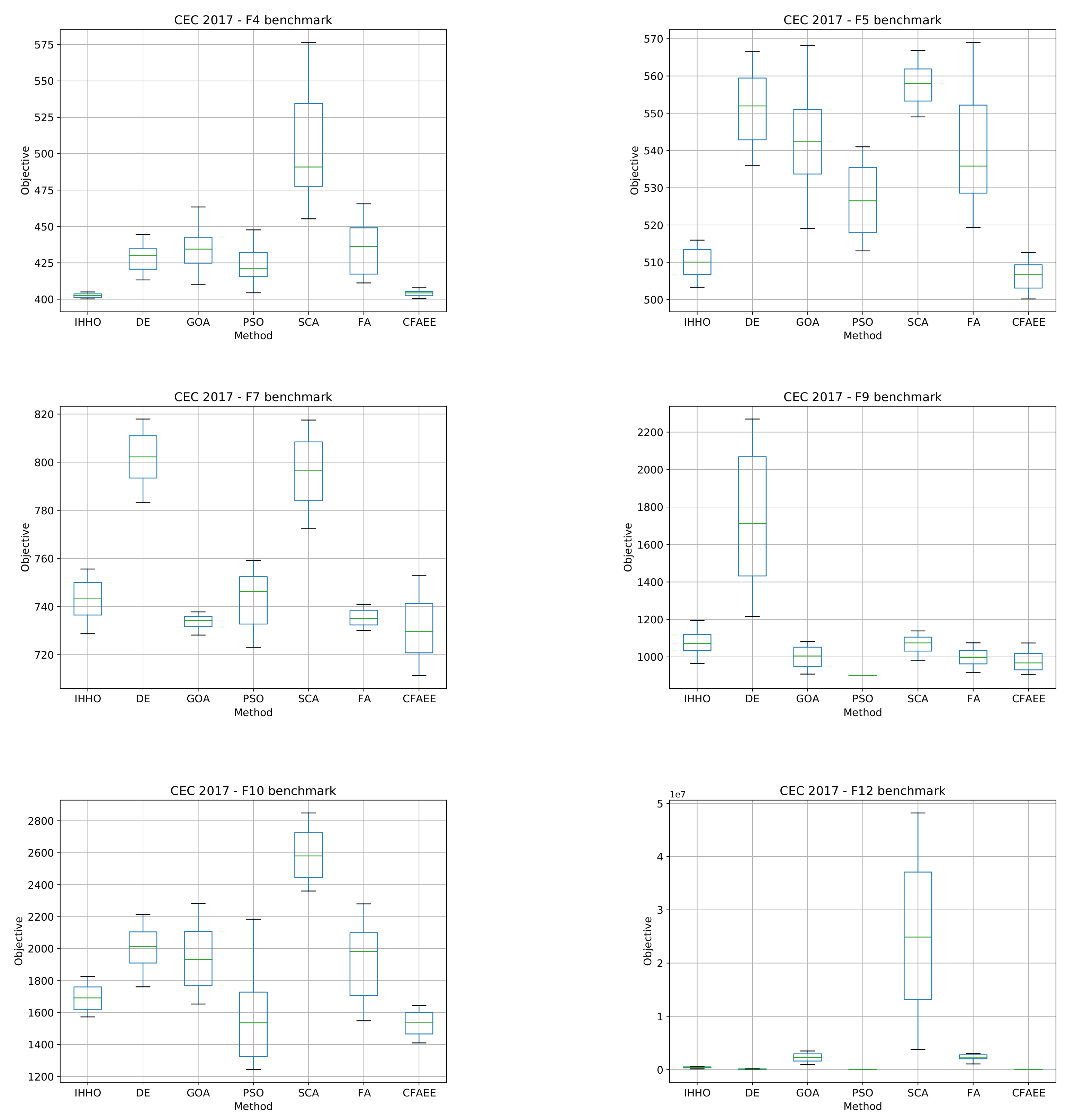
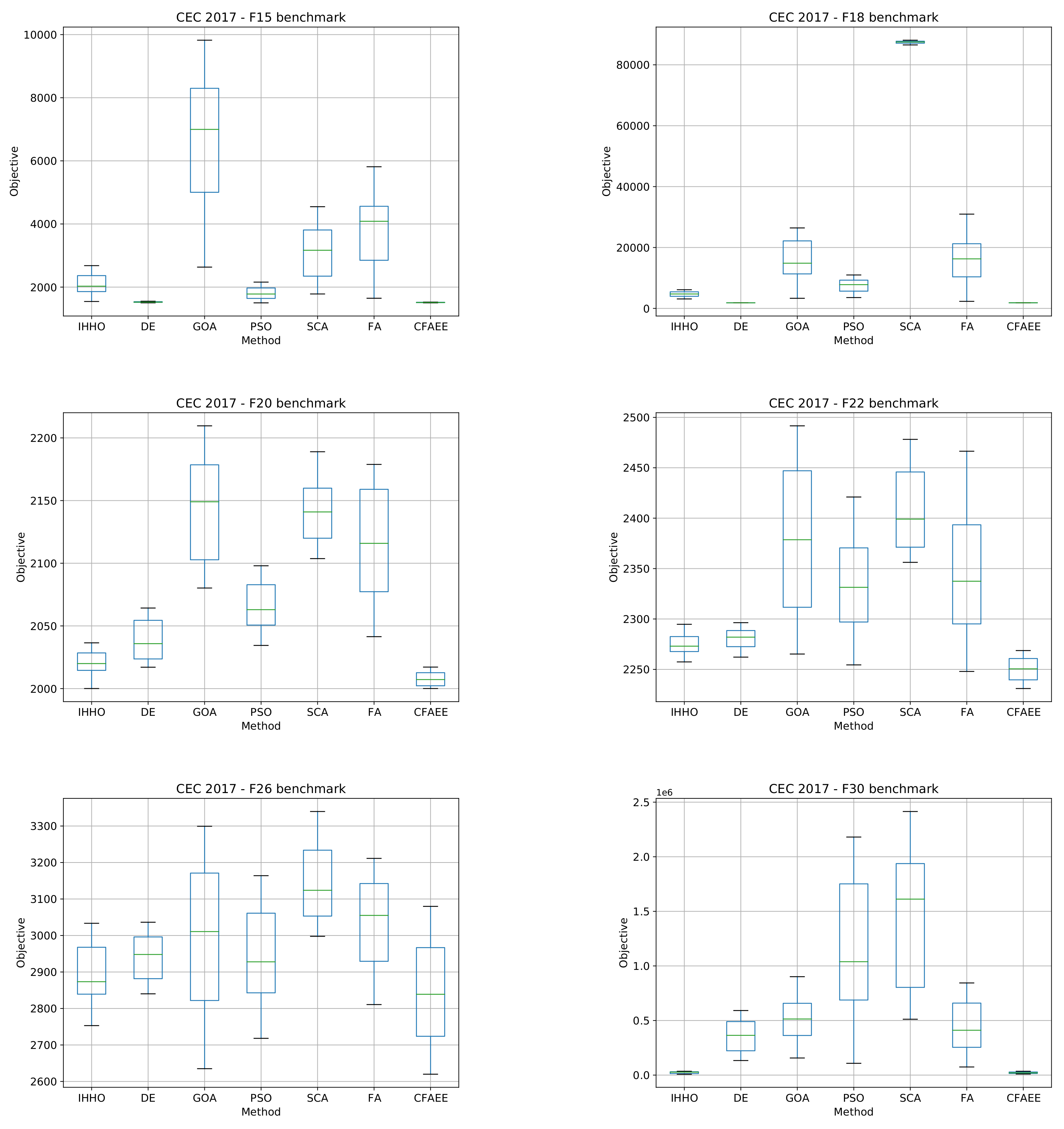
4.3. Benchmark Problem Set 2

The second bound-constrained validation of the proposed CFAEE was conducted on a very challenging CEC 2017 benchmark suite [59]. The suite is composed of 30 benchmarks divided into 4 groups: $F1–F3$ are uni-modal, $F4–F10$ are multi-modal, $F11–F20$ belong to the class of hybrid functions, while tests $F21–F30$ are very challenging composite functions. The last group contains properties of all uni-modal, multi-modal, and hybrid functions; moreover, they are shifted and rotated.

Test instance $F2$ was deleted from the test suite due to unstable behavior [60], and these results are not reported. Basic details of CEC 2017 instances are given in

Table 9. CEC 2017 function details.

ID	Name of the function	Class	Search Range	Optimum
F1	Shifted and Rotated Bent Cigar Function	Unimodal	[−100, 100]	100
F2	Shifted and Rotated Sum of Different Power Function	Unimodal	[−100, 100]	200
F3	Shifted and Rotated Zakharov Function	Unimodal	[−100, 100]	300
F4	Shifted and Rotated Rosenbrock’s Function	Multimodal	[−100, 100]	400
F5	Shifted and Rotated Rastrigin’s Function	Multimodal	[−100, 100]	500
F6	Shifted and Rotated Expanded Scaffer’s Function	Multimodal	[−100, 100]	600
F7	Shifted and Rotated Lunacek Bi-Rastrigin Function	Multimodal	[−100, 100]	700
F8	Shifted and Rotated Non-Continuous Rastrigin’s Function	Multimodal	[−100, 100]	800
F9	Shifted and Rotated Lévy Function	Multimodal	[−100, 100]	900
F10	Shifted and Rotated Schwefel’s Function	Multimodal	[−100, 100]	1000
F11	Hybrid Function 1 (N = 3)	Hybrid	[−100, 100]	1100
F12	Hybrid Function 2 (N = 3)	Hybrid	[−100, 100]	1200
F13	Hybrid Function 3 (N = 3)	Hybrid	[−100, 100]	1300
F14	Hybrid Function 4 (N = 4)	Hybrid	[−100, 100]	1400
F15	Hybrid Function 5 (N = 4)	Hybrid	[−100, 100]	1500
F16	Hybrid Function 6 (N = 4)	Hybrid	[−100, 100]	1600
F17	Hybrid Function 6 (N = 5)	Hybrid	[−100, 100]	1700
F18	Hybrid Function 6 (N = 5)	Hybrid	[−100, 100]	1800
F19	Hybrid Function 6 (N = 5)	Hybrid	[−100, 100]	1900
F20	Hybrid Function 6 (N = 6)	Hybrid	[−100, 100]	2000
F21	Composition Function 1 (N = 3)	Composition	[−100, 100]	2100
F22	Composition Function 2 (N = 3)	Composition	[−100, 100]	2200
F23	Composition Function 3 (N = 4)	Composition	[−100, 100]	2300
F24	Composition Function 4 (N = 4)	Composition	[−100, 100]	2400
F25	Composition Function 5 (N = 5)	Composition	[−100, 100]	2500
F26	Composition Function 6 (N = 5)	Composition	[−100, 100]	2600
F27	Composition Function 7 (N = 6)	Composition	[−100, 100]	2700
F28	Composition Function 8 (N = 6)	Composition	[−100, 100]	2800
F29	Composition Function 9 (N = 3)	Composition	[−100, 100]	2900
F30	Composition Function 10 (N = 3)	Composition	[−100, 100]	3000

.

Simulations are executed with 30-dimensional instances ($D=30$) and mean (average) and standard deviation (std) results for 50 runs are reported. The proposed CFAEE is compared against the basic FA with dynamic $\alpha$, state-of-the-art improved Harris hawks optimization (IHHO) presented in [61], and other well-known efficient nature-inspired metaheuristics: HHO, DE, GOA, GWO, MFO, MVO, PSO, WOA, and SCA.

In this study, the same experimental setup as in [61] was recreated. The study shown in [61] reports results with $N=30$ and $T=500$. However, as in the case of the first unconstrained experiment, since the CFAEE utilizes more $FFE$ in each run, the $maxFFE$ is used as the termination criteria. All approaches included in the comparative analysis employ one $FFE$ per solution in the initialization and update phases, and to conduct an unbiased comparison, $maxFFE$ was set to 15,030 ($N+N·T$). Control parameter adjustments of opponent methods can be retrieved from [61].

Comparative analysis results for the CEC 2017 benchmark suite are reported in

Table 10. CEC 2017 comparative analysis results.

Algorithm	F1		F2		F3		F4		F5
	Mean	STD	Mean	STD	Mean	STD	Mean	STD	Mean	STD
IHHO	$1.86\times {10}^{+2}$	26.921	n/a	n/a	3.02$\times {10}^{+2}$	52.152	4.03$\times {10}^{+2}$	2.607	$5.05\times {10}^{+2}$	3.251
HHO	$1.75\times {10}^{+6}$	$4.29\times {10}^{+5}$	n/a	n/a	$6.71\times {10}^{+2}$	$3.24\times {10}^{+2}$	$4.37\times {10}^{+2}$	53.631	$5.35\times {10}^{+2}$	24.927
DE	$7.54\times {10}^{+7}$	$1.71\times {10}^{+7}$	n/a	n/a	$4.59\times {10}^{+3}$	$1.35\times {10}^{+3}$	$4.29\times {10}^{+2}$	8.530	$5.52\times {10}^{+2}$	6.232
GOA	$1.56\times {10}^{+5}$	$5.24\times {10}^{+4}$	n/a	n/a	$3.05\times {10}^{+2}$	61.300	$4.15\times {10}^{+2}$	19.48	$5.25\times {10}^{+2}$	16.803
GWO	$1.53\times {10}^{+7}$	$4.85\times {10}^{+6}$	n/a	n/a	$3.57\times {10}^{+3}$	$2.77\times {10}^{+3}$	$4.09\times {10}^{+2}$	10.705	$5.19\times {10}^{+2}$	8.543
MFO	$7.17\times {10}^{+6}$	$2.18\times {10}^{+7}$	n/a	n/a	$9.04\times {10}^{+3}$	$9.31\times {10}^{+3}$	$4.20\times {10}^{+2}$	27.727	$5.31\times {10}^{+2}$	12.860
MVO	$1.79\times {10}^{+4}$	$7.99\times {10}^{+3}$	n/a	n/a	$3.05\times {10}^{+2}$	46.451	$4.06\times {10}^{+2}$	1.392	$5.17\times {10}^{+2}$	9.888
PSO	$9.49\times {10}^{+4}$	$8.42\times {10}^{+2}$	n/a	n/a	$3.49\times {10}^{+2}$	65.409	$4.07\times {10}^{+2}$	10.318	$5.26\times {10}^{+2}$	7.305
WOA	$4.27\times {10}^{+7}$	$3.81\times {10}^{+6}$	n/a	n/a	$5.16\times {10}^{+3}$	$4.22\times {10}^{+2}$	$4.61\times {10}^{+2}$	69.033	$5.51\times {10}^{+2}$	17.46
SCA	$1.15\times {10}^{+8}$	$5.91\times {10}^{+7}$	n/a	n/a	$4.03\times {10}^{+3}$	$8.42\times {10}^{+2}$	$4.85\times {10}^{+2}$	47.271	$5.59\times {10}^{+2}$	9.352
FA	$1.61\times {10}^{+5}$	$3.77\times {10}^{+4}$	n/a	n/a	$3.09\times {10}^{+2}$	54.991	$4.17\times {10}^{+2}$	18.858	$5.28\times {10}^{+2}$	19.302
CFAEE	1.31$\times {10}^{+2}$	14.353	n/a	n/a	3.02$\times {10}^{+2}$	28.131	$4.04\times {10}^{+2}$	2.372	5.01$\times {10}^{+2}$	3.285
Algorithm	F6		F7		F8		F9		F10
	Mean	STD	Mean	STD	Mean	STD	Mean	STD	Mean	STD
IHHO	6.00$\times {10}^{+2}$	0.082	$7.49\times {10}^{+2}$	10.041	$8.11\times {10}^{+2}$	6.526	$1.13\times {10}^{+3}$	85.42	$1.69\times {10}^{+3}$	$1.31\times {10}^{+2}$
HHO	$6.38\times {10}^{+2}$	12.320	$7.96\times {10}^{+2}$	18.921	$8.29\times {10}^{+2}$	5.700	$1.44\times {10}^{+3}$	$1.24\times {10}^{+2}$	$2.03\times {10}^{+3}$	$3.42\times {10}^{+2}$
DE	$6.28\times {10}^{+2}$	4.744	$8.01\times {10}^{+2}$	10.373	$8.62\times {10}^{+2}$	6.873	$1.76\times {10}^{+3}$	$1.48\times {10}^{+2}$	$2.09\times {10}^{+3}$	$2.01\times {10}^{+2}$
GOA	$6.08\times {10}^{+2}$	10.295	$7.32\times {10}^{+2}$	11.375	$8.31\times {10}^{+2}$	14.512	$9.97\times {10}^{+2}$	93.212	$1.96\times {10}^{+3}$	$3.17\times {10}^{+2}$
GWO	$6.01\times {10}^{+2}$	1.909	$7.35\times {10}^{+2}$	16.343	$8.16\times {10}^{+2}$	5.053	$9.14\times {10}^{+2}$	12.11	$1.76\times {10}^{+3}$	$3.10\times {10}^{+2}$
MFO	$6.02\times {10}^{+2}$	2.411	$7.46\times {10}^{+2}$	22.655	$8.29\times {10}^{+2}$	13.786	$1.23\times {10}^{+3}$	$2.76\times {10}^{+2}$	$2.02\times {10}^{+3}$	$3.27\times {10}^{+2}$
MVO	$6.03\times {10}^{+2}$	4.365	$7.30\times {10}^{+2}$	11.278	$8.25\times {10}^{+2}$	12.216	9.00$\times {10}^{+2}$	0.012	$1.82\times {10}^{+3}$	$3.60\times {10}^{+2}$
PSO	$6.10\times {10}^{+2}$	3.539	$7.26\times {10}^{+2}$	9.008	$8.19\times {10}^{+2}$	5.982	9.00$\times {10}^{+2}$	0.003	1.50$\times {10}^{+3}$	$2.84\times {10}^{+2}$
WOA	$6.36\times {10}^{+2}$	13.695	$7.82\times {10}^{+2}$	23.692	$8.45\times {10}^{+2}$	17.470	$1.54\times {10}^{+3}$	$3.94\times {10}^{+2}$	$2.19\times {10}^{+3}$	$3.16\times {10}^{+2}$
SCA	$6.24\times {10}^{+2}$	4.105	$7.84\times {10}^{+2}$	13.299	$8.47\times {10}^{+2}$	7.577	$1.03\times {10}^{+3}$	85.98	$2.51\times {10}^{+3}$	$2.18\times {10}^{+2}$
FA	$6.71\times {10}^{+2}$	11.393	$7.35\times {10}^{+2}$	11.55	$8.33\times {10}^{+2}$	13.914	$9.97\times {10}^{+2}$	81.44	$1.93\times {10}^{+3}$	$2.96\times {10}^{+2}$
CFAEE	6.00$\times {10}^{+2}$	0.051	7.23$\times {10}^{+2}$	11.391	8.08$\times {10}^{+2}$	5.422	$9.87\times {10}^{+2}$	42.11	$1.58\times {10}^{+3}$	1.25$\times {10}^{+2}$
Algorithm	F11		F12		F13		F14		F15
	Mean	STD	Mean	STD	Mean	STD	Mean	STD	Mean	STD
IHHO	$1.12\times {10}^{+3}$	13.523	$4.25\times {10}^{+5}$	$3.05\times {10}^{+5}$	$4.42\times {10}^{+3}$	$2.18\times {10}^{+3}$	1.42$\times {10}^{+3}$	1.651	$2.15\times {10}^{+3}$	$5.65\times {10}^{+2}$
HHO	$1.16\times {10}^{+3}$	45.729	$2.56\times {10}^{+6}$	$1.13\times {10}^{+6}$	$1.92\times {10}^{+4}$	$1.16\times {10}^{+4}$	$1.83\times {10}^{+3}$	$2.41\times {10}^{+2}$	$8.63\times {10}^{+3}$	$5.55\times {10}^{+2}$
DE	$1.14\times {10}^{+3}$	36.317	$9.15\times {10}^{+4}$	$6.58\times {10}^{+4}$	1.35$\times {10}^{+3}$	78.355	$1.46\times {10}^{+3}$	11.826	1.51$\times {10}^{+3}$	18.454
GOA	$1.17\times {10}^{+3}$	58.009	$2.24\times {10}^{+6}$	$1.15\times {10}^{+6}$	$1.65\times {10}^{+4}$	$1.13\times {10}^{+4}$	$2.93\times {10}^{+3}$	$1.15\times {10}^{+3}$	$6.48\times {10}^{+3}$	$4.32\times {10}^{+3}$
GWO	$1.34\times {10}^{+3}$	183.524	$1.31\times {10}^{+6}$	$1.54\times {10}^{+6}$	$1.26\times {10}^{+4}$	$7.82\times {10}^{+3}$	$3.19\times {10}^{+3}$	$1.82\times {10}^{+3}$	$5.63\times {10}^{+3}$	$3.16\times {10}^{+3}$
MFO	$1.23\times {10}^{+3}$	107.133	$2.23\times {10}^{+6}$	$4.81\times {10}^{+6}$	$1.61\times {10}^{+4}$	$1.39\times {10}^{+4}$	$8.42\times {10}^{+3}$	$5.42\times {10}^{+3}$	$1.25\times {10}^{+4}$	$1.02\times {10}^{+4}$
MVO	$1.14\times {10}^{+3}$	27.331	$1.52\times {10}^{+6}$	$1.41\times {10}^{+6}$	$9.89\times {10}^{+3}$	$2.55\times {10}^{+3}$	$2.15\times {10}^{+3}$	$1.03\times {10}^{+3}$	$4.05\times {10}^{+3}$	$2.45\times {10}^{+3}$
PSO	1.10$\times {10}^{+3}$	3.727	$4.35\times {10}^{+4}$	$1.26\times {10}^{+4}$	$1.01\times {10}^{+4}$	$7.23\times {10}^{+3}$	$1.49\times {10}^{+3}$	88.291	$1.81\times {10}^{+3}$	$3.75\times {10}^{+2}$
WOA	$1.22\times {10}^{+3}$	82.415	$4.85\times {10}^{+6}$	$5.12\times {10}^{+6}$	$1.57\times {10}^{+4}$	$1.38\times {10}^{+4}$	$3.42\times {10}^{+3}$	$9.82\times {10}^{+2}$	$1.42\times {10}^{+4}$	$9.88\times {10}^{+3}$
SCA	$1.24\times {10}^{+3}$	96.535	$2.41\times {10}^{+7}$	$2.05\times {10}^{+7}$	$6.43\times {10}^{+4}$	$4.69\times {10}^{+4}$	$1.99\times {10}^{+3}$	$4.31\times {10}^{+2}$	$3.21\times {10}^{+3}$	$1.41\times {10}^{+3}$
FA	$1.16\times {10}^{+3}$	39.705	$2.32\times {10}^{+6}$	$1.21\times {10}^{+6}$	$1.21\times {10}^{+4}$	$1.05\times {10}^{+4}$	$1.88\times {10}^{+3}$	$3.21\times {10}^{+2}$	$3.67\times {10}^{+3}$	$2.13\times {10}^{+3}$
CFAEE	1.10$\times {10}^{+3}$	1.503	3.18$\times {10}^{+4}$	2.29$\times {10}^{+4}$	1.35$\times {10}^{+3}$	20.499	$1.43\times {10}^{+3}$	21.350	1.51$\times {10}^{+3}$	10.217
Algorithm	F16		F17		F18		F19		F20
	Mean	STD	Mean	STD	Mean	STD	Mean	STD	Mean	STD
IHHO	$1.73\times {10}^{+3}$	59.44	$1.73\times {10}^{+3}$	7.519	$4.79\times {10}^{+3}$	$1.68\times {10}^{+3}$	1.90$\times {10}^{+3}$	6.993	$2.02\times {10}^{+3}$	19.561
HHO	$1.89\times {10}^{+3}$	$1.47\times {10}^{+2}$	$1.79\times {10}^{+3}$	65.751	$2.02\times {10}^{+4}$	$1.41\times {10}^{+4}$	$1.71\times {10}^{+4}$	$1.21\times {10}^{+4}$	$2.23\times {10}^{+3}$	86.017
DE	$1.69\times {10}^{+3}$	41.15	$1.77\times {10}^{+3}$	19.514	1.84$\times {10}^{+3}$	23.298	$2.75\times {10}^{+3}$	$8.35\times {10}^{+2}$	$2.05\times {10}^{+3}$	23.711
GOA	$1.78\times {10}^{+3}$	$1.76\times {10}^{+2}$	$1.83\times {10}^{+3}$	$1.21\times {10}^{+2}$	$1.63\times {10}^{+4}$	$1.31\times {10}^{+4}$	$3.25\times {10}^{+3}$	$1.95\times {10}^{+3}$	$2.15\times {10}^{+3}$	74.824
GWO	$1.79\times {10}^{+3}$	$1.11\times {10}^{+2}$	$1.77\times {10}^{+3}$	38.759	$2.55\times {10}^{+4}$	$1.84\times {10}^{+4}$	$2.75\times {10}^{+4}$	$2.38\times {10}^{+4}$	$2.09\times {10}^{+3}$	73.994
MFO	$1.85\times {10}^{+3}$	$15.23\times {10}^{+2}$	$1.78\times {10}^{+3}$	65.311	$2.21\times {10}^{+4}$	$1.39\times {10}^{+4}$	$7.81\times {10}^{+3}$	$6.15\times {10}^{+3}$	$2.13\times {10}^{+3}$	72.321
MVO	$1.80\times {10}^{+3}$	$1.44\times {10}^{+2}$	$1.80\times {10}^{+3}$	46.126	$2.03\times {10}^{+4}$	$1.25\times {10}^{+4}$	$4.63\times {10}^{+3}$	$2.62\times {10}^{+3}$	$2.12\times {10}^{+3}$	86.303
PSO	1.65$\times {10}^{+3}$	65.364	$1.72\times {10}^{+3}$	16.123	$7.63\times {10}^{+3}$	$4.46\times {10}^{+3}$	$3.13\times {10}^{+3}$	$2.05\times {10}^{+3}$	$2.06\times {10}^{+3}$	35.410
WOA	$1.96\times {10}^{+3}$	$14.92\times {10}^{+2}$	$1.82\times {10}^{+3}$	73.459	$2.13\times {10}^{+4}$	$1.95\times {10}^{+2}$	$2.07\times {10}^{+5}$	$1.16\times {10}^{+5}$	$2.19\times {10}^{+3}$	$1.11\times {10}^{+2}$
SCA	$1.73\times {10}^{+3}$	95.425	$1.80\times {10}^{+3}$	$25.30\times {10}^3$	$8.77\times {10}^{+4}$	$9.23\times {10}^{+2}$	$1.15\times {10}^{+4}$	$1.44\times {10}^{+3}$	$2.14\times {10}^{+3}$	46.855
FA	$1.79\times {10}^{+3}$	$1.73\times {10}^{+2}$	$1.82\times {10}^{+3}$	$1.15\times {10}^{+2}$	$1.67\times {10}^{+4}$	$1.45\times {10}^{+4}$	$3.18\times {10}^{+3}$	$1.59\times {10}^{+3}$	$2.12\times {10}^{+3}$	71.303
CFAEE	$1.70\times {10}^{+3}$	86.359	1.71$\times {10}^{+3}$	8.442	$1.86\times {10}^{+3}$	21.565	1.90$\times {10}^{+3}$	8.717	2.01$\times {10}^{+3}$	9.443
Algorithm	F21		F22		F23		F24		F25
	Mean	STD	Mean	STD	Mean	STD	Mean	STD	Mean	STD
IHHO	2.20$\times {10}^{+3}$	4.615	$2.28\times {10}^{+3}$	17.820	$2.59\times {10}^{+3}$	14.213	$2.68\times {10}^{+3}$	$1.31\times {10}^{+2}$	$2.87\times {10}^{+3}$	85.338
HHO	$2.35\times {10}^{+3}$	53.711	$2.32\times {10}^{+3}$	25.234	$2.69\times {10}^{+3}$	35.522	$2.82\times {10}^{+3}$	93.623	$2.95\times {10}^{+3}$	49.573
DE	$2.25\times {10}^{+3}$	78.104	$2.29\times {10}^{+3}$	17.513	$2.63\times {10}^{+3}$	15.163	2.66$\times {10}^{+3}$	69.502	$2.91\times {10}^{+3}$	15.543
GOA	$2.30\times {10}^{+3}$	56.877	$2.38\times {10}^{+3}$	$1.08\times {10}^{+2}$	$2.64\times {10}^{+3}$	23.536	$2.73\times {10}^{+3}$	57.833	$2.93\times {10}^{+3}$	32.598
GWO	$2.30\times {10}^{+3}$	32.884	$2.31\times {10}^{+3}$	57.573	$2.62\times {10}^{+3}$	13.862	$2.74\times {10}^{+3}$	25.132	$2.94\times {10}^{+3}$	28.256
MFO	$2.32\times {10}^{+3}$	29.255	$2.35\times {10}^{+3}$	93.557	$2.63\times {10}^{+3}$	11.327	$2.75\times {10}^{+3}$	76.435	$2.96\times {10}^{+3}$	37.776
MVO	$2.32\times {10}^{+3}$	11.839	$2.33\times {10}^{+3}$	$1.11\times {10}^{+2}$	$2.65\times {10}^{+3}$	10.445	$2.74\times {10}^{+3}$	18.246	$2.92\times {10}^{+3}$	84.256
PSO	$2.27\times {10}^{+3}$	49.783	$2.33\times {10}^{+3}$	$1.03\times {10}^{+2}$	$2.60\times {10}^{+3}$	72.300	$2.70\times {10}^{+3}$	76.143	$2.90\times {10}^{+3}$	33.735
WOA	$2.34\times {10}^{+3}$	60.021	$2.48\times {10}^{+3}$	$2.45\times {10}^{+2}$	$2.66\times {10}^{+3}$	29.838	$2.77\times {10}^{+3}$	85.902	$2.98\times {10}^{+3}$	$1.03\times {10}^{+2}$
SCA	$2.29\times {10}^{+3}$	65.229	$2.41\times {10}^{+3}$	66.636	$2.67\times {10}^{+3}$	45.449	$2.78\times {10}^{+3}$	11.548	$2.98\times {10}^{+3}$	37.291
FA	$2.29\times {10}^{+3}$	34.701	$2.36\times {10}^{+3}$	$1.10\times {10}^{+2}$	$2.62\times {10}^{+3}$	17.452	$2.72\times {10}^{+3}$	$1.05\times {10}^{+2}$	$2.93\times {10}^{+3}$	47.019
CFAEE	2.20$\times {10}^{+3}$	48.552	2.26$\times {10}^{+3}$	13.040	2.55$\times {10}^{+3}$	21.929	$2.67\times {10}^{+3}$	$1.72\times {10}^{+2}$	2.81$\times {10}^{+3}$	95.429
Algorithm	F26		F27		F28		F29		F30
	Mean	STD	Mean	STD	Mean	STD	Mean	STD	Mean	STD
IHHO	$2.93\times {10}^{+3}$	$1.66\times {10}^{+2}$	$3.19\times {10}^{+3}$	33.657	$3.30\times {10}^{+3}$	48.694	3.20$\times {10}^{+3}$	28.982	$2.30\times {10}^{+4}$	$1.45\times {10}^{+4}$
HHO	$3.62\times {10}^{+3}$	$5.39\times {10}^{+2}$	$3.18\times {10}^{+3}$	51.306	$3.41\times {10}^{+3}$	$1.02\times {10}^{+2}$	$3.39\times {10}^{+3}$	85.653	$1.43\times {10}^{+6}$	$1.31\times {10}^{+6}$
DE	$2.95\times {10}^{+3}$	95.929	3.07$\times {10}^{+3}$	2.558	$3.28\times {10}^{+3}$	27.035	$3.21\times {10}^{+3}$	35.216	$3.65\times {10}^{+5}$	$2.31\times {10}^{+5}$
GOA	$3.01\times {10}^{+3}$	$3.65\times {10}^{+2}$	$3.11\times {10}^{+3}$	25.326	$3.31\times {10}^{+3}$	$1.53\times {10}^{+2}$	$3.27\times {10}^{+3}$	75.411	$5.29\times {10}^{+5}$	$3.89\times {10}^{+5}$
GWO	$3.36\times {10}^{+3}$	$5.05\times {10}^{+2}$	$3.10\times {10}^{+3}$	13.541	$3.42\times {10}^{+3}$	$1.33\times {10}^{+2}$	$3.22\times {10}^{+3}$	49.822	$6.17\times {10}^{+5}$	$4.88\times {10}^{+5}$
MFO	$3.05\times {10}^{+3}$	$1.13\times {10}^{+2}$	$3.09\times {10}^{+3}$	5.722	$3.21\times {10}^{+3}$	93.459	$3.26\times {10}^{+3}$	55.593	$6.36\times {10}^{+5}$	$5.93\times {10}^{+5}$
MVO	$3.15\times {10}^{+3}$	$2.77\times {10}^{+2}$	$3.10\times {10}^{+3}$	21.875	$3.36\times {10}^{+3}$	$1.23\times {10}^{+2}$	$3.26\times {10}^{+3}$	75.139	$4.62\times {10}^{+5}$	$4.07\times {10}^{+5}$
PSO	$2.95\times {10}^{+3}$	$2.55\times {10}^{+2}$	$3.12\times {10}^{+3}$	31.830	$3.32\times {10}^{+3}$	$1.35\times {10}^{+2}$	$3.21\times {10}^{+3}$	62.374	$1.13\times {10}^{+6}$	$1.09\times {10}^{+6}$
WOA	$3.37\times {10}^{+3}$	$2.92\times {10}^{+2}$	$3.17\times {10}^{+3}$	48.124	$3.46\times {10}^{+3}$	$1.65\times {10}^{+2}$	$3.46\times {10}^{+3}$	$1.21\times {10}^{+2}$	$1.29\times {10}^{+6}$	$7.53\times {10}^{+5}$
SCA	$3.15\times {10}^{+3}$	$1.82\times {10}^{+2}$	$3.13\times {10}^{+3}$	13.152	$3.38\times {10}^{+3}$	89.259	$3.25\times {10}^{+3}$	48.339	$1.49\times {10}^{+6}$	$9.77\times {10}^{+5}$
FA	$3.02\times {10}^{+3}$	$2.03\times {10}^{+2}$	$3.10\times {10}^{+3}$	27.015	$3.32\times {10}^{+3}$	$1.17\times {10}^{+2}$	$3.26\times {10}^{+3}$	31.117	$4.71\times {10}^{+5}$	$4.02\times {10}^{+5}$
CFAEE	2.86$\times {10}^{+3}$	$2.45\times {10}^{+2}$	$3.08\times {10}^{+3}$	48.690	3.13$\times {10}^{+3}$	$2.51\times {10}^{+2}$	3.20$\times {10}^{+3}$	27.914	2.22$\times {10}^{+4}$	1.44$\times {10}^{+4}$

. The best results for each performance indicator and instance are marked bold. Moreover, if two or more algorithms obtained the same performance, which are the best at the same time, these results are also underlined. Very similar results as in [54] are obtained, but with subtle discrepancies due to the stochastic nature metaheuristics.

The Table 10 shows that the CFAEE had the best results over 21 functions; those were F1, F3, F5, F6, F7, F8, F11, F12, F13, F15, F17, F19, F20, F21, F22, F23, F25, F26, F28, F29, and F30. In some cases, these case algorithms had the best results, but they were tied with results from another algorithm. In these cases, both results are in bold. The algorithm outperformed every other algorithm in these cases and the IHHO.

With some functions from the previously mentioned set, the CFAEE had the same results as the IHHO, and in those situations, they were tied as having the best results. Such cases are F3, F6, F19, F21, and F29. These results are underlined and in bold. It can be observed that, not only CFAEE and IHHO were tied with their results, from some functions; these results are also underlined and in bold. For function F9, the two best algorithms were MVO and PSO. The results of CFAEE and PSO were also tied (for function F11) as having the best results. Finally, with functions F13 and F15, the CFAEE was tied with the DE as having the best results.

In the minority of cases, the CFAEE was outperformed by the IHHO and other algorithms. The IHHO algorithm was only better for functions F4 and F14. The alternative best solutions only came from PSO, MVO, and DE. The previously mentioned case of PSO and MVO, being tied as having the best result with function F9, is one of them; two other cases where PSO was best were with functions F10 and F16. The only other algorithm that was better is the DE, in cases of F18, F24, and F27.

It is important to note that, in no case, was the original FA better than the improved version CFAEE. For some functions, the CFAEE achieved vastly improved results, as much as more than 1000 times better, as seen in F1. Large differences can be seen with other functions as well, such as F12, F13, F18, and F30.

Considering all of the mentioned cases, there is no doubt that the proposed solution, CFAEE, is superior to the original solution, FA, but also to every other algorithm tested. Furthermore, the improvement is justified.

The Friedman test [62,63] and the two-way variance analysis, by ranks, were performed for the determination of the difference significance between the novel CFAEE and the alternative methods used for comparison. This was conducted to further establish the statistical significance of enhancements, not only by comparing the results.

Table 11. Friedman test ranks for the compared algorithms over 30 CEC2017 functions.

Function	IHHO	HHO	DE	GOA	GWO	MFO	MVO	PSO	WOA	SCA	FA	CFAEE
F1	2	7	11	5	9	8	3	4	10	12	6	1
F3	1.5	7	10	3.5	8	12	3.5	6	11	9	5	1.5
F4	1	10	9	6	5	8	3	4	11	12	7	2
F5	2	9	11	5	4	8	3	6	10	12	7	1
F6	1.5	11	9	6	3	4	5	7	10	8	12	1.5
F7	8	11	12	4	5.5	7	3	2	9	10	5.5	1
F8	2	6.5	12	8	3	6.5	5	4	10	11	9	1
F9	8	10	12	5.5	3	9	1.5	1.5	11	7	5.5	4
F10	3	9	10	7	4	8	5	1	11	12	6	2
F11	3	6.5	4.5	8	12	10	4.5	1.5	9	11	6.5	1.5
F12	4	10	3	8	5	7	6	2	11	12	9	1
F13	3	11	1.5	10	7	9	4	5	8	12	6	1.5
F14	1	5	3	9	10	12	8	4	11	7	6	2
F15	4	10	1.5	9	8	11	7	3	12	5	6	1.5
F16	5.5	11	3	1	7.5	10	9	2	12	5.5	7.5	4
F17	3	7	4.5	12	4.5	6	8.5	2	10.5	8.5	10.5	1
F18	3	7	1	5	11	10	8	4	9	12	6	2
F19	1.5	10	3	6	11	8	7	4	12	9	5	1.5
F20	2	12	3	10	5	8	6.5	4	11	9	6.5	1
F21	1.5	12	3	7.5	7.5	9.5	9.5	4	11	5.5	5.5	1.5
F22	2	5	3	10	4	8	6.5	6.5	12	11	9	1
F23	2	12	6.5	8	4.5	6.5	9	3	10	11	4.5	1
F24	3	12	1	6	7.5	9	7.5	4	10	11	5	2
F25	2	9	4	6.5	8	10	5	3	11.5	11.5	6.5	1
F26	2	12	3.5	5	10	7	8.5	3.5	11	8.5	6	1
F27	12	11	1	7	5	3	5	8	10	9	5	2
F28	4	10	3	5	11	2	8	6.5	12	9	6.5	1
F29	1.5	11	3.5	10	5	8	8	3.5	12	6	8	1.5
F30	2	11	3	6	7	8	4	9	10	12	5	1
Average Ranking	3.138	9.483	5.362	6.862	6.724	8.017	5.914	4.069	10.621	9.603	6.655	1.552
Rank	2	10	4	8	7	9	5	3	12	11	6	1

and

Table 12. Aligned Friedman test ranks for the compared algorithms over 30 CEC2017 functions.

Function	IHHO	HHO	DE	GOA	GWO	MFO	MVO	PSO	WOA	SCA	FA	CFAEE
F1	2	7	347	5	9	8	3	4	346	348	6	1
F3	56.5	63	327	58.5	323	334	58.5	61	328	326	60	56.5
F4	144	226	211	177	164	192	152	157	255	278	183	146
F5	138	213	242	194	174	206	169	196	241	245	197	135
F6	153.5	235	218	173	158	161	165	180	232	212	270	153.5
F7	193	264	266	145	155.5	184	140	136	244	246	155.5	131
F8	151	198.5	251	204	167	198.5	191	172	229	231	207	143
F9	141	310	318	89.5	80	285	78.5	78.5	313	91	89.5	87
F10	81	293	301	257	88	290	95	74	309	317	216	75
F11	114	159.5	127.5	185	300	271	127.5	103.5	265	280	159.5	103.5
F12	13	19	12	17	14	16	15	11	344	345	18	10
F13	43	331	39.5	324	54	321	45	46	314	337	53	39.5
F14	66	70	68	311	316	333	73	69	320	72	71	67
F15	52	329	48.5	322	303	335	65	51	336	55	62	48.5
F16	291.5	308	276	64	298.5	305	302	233	312	291.5	298.5	282
F17	122	225	181.5	269	181.5	205	239.5	113	262.5	239.5	262.5	107
F18	38	76	35	47	332	325	82	41	319	338	50	36
F19	28.5	44	30	33	330	37	34	31	339	42	32	28.5
F20	98	294	112	260.5	150	237.5	223	121	286	247.5	223	96
F21	99.5	281	129	227.5	227.5	252.5	252.5	162.5	272	209	209	99.5
F22	110	142	118	258	130	217	170.5	170.5	297	283	234	101
F23	126	279	202.5	223	178.5	202.5	237.5	134	247.5	260.5	178.5	102
F24	119.5	288	105	200.5	220	236	220	132.5	259	267.5	175.5	111
F25	117	243	168	214.5	230	256	195	139	274.5	274.5	214.5	93
F26	84	315	85.5	94	306	106	249.5	85.5	307	249.5	97	77
F27	284	277	119.5	175.5	148	132.5	148	200.5	267.5	220	148	125
F28	137	287	124	166	289	92	254	189.5	296	273	189.5	83
F29	108.5	295	115.5	209	123	187	187	115.5	304	162.5	187	108.5
F30	21	342	22	25	26	27	23	340	341	343	24	20
Average Ranking	108.017	221.172	158.621	169.948	188.810	205.259	144.655	122.328	291.724	244.276	147.259	91.931
Rank	2	10	6	7	8	9	4	3	12	11	5	1

present the results achieved by 12 different algorithms over the 30 functions from the CEC2017 set for Friedman test ranks and the aligned Friedman test ranks, respectively.

As seen in Table 11, one could conclude that the proposed method, CFAEE, achieves better performance than the 10 other algorithms, as well as the original FA. The original HHO algorithm had an average ranking of 9.483. The modified version of HHO, the IHHO, had 3.138. The original FA had 6.655. The improved CFAEE was more than twice better than the previous best solution of IHHO with the average ranking of 1.551.

Additionally, the Iman and Davenport test [64] was also performed because the research [65] proves that the test could possibly provide better results in terms of precision than the ${\chi }^2$. Summary of the results from Friedman and Iman and Davenport’s test can be seen in

Table 13. Friedman and Iman–Davenport statistical test results summary ($\alpha =0.05$).

Friedman Value	${\mathit{\chi }}^2$ Critical Value	p-Value	Iman–Davenport Value	F Critical Value
$1.815\times {10}^{+2}$	$1.968\times {10}^{+1}$	$1.110\times {10}^{-16}$	$3.695\times {10}^{+1}$	1.820

.

Upon completion of the calculations, the result of the Iman and Davenport test is $36.95$ and put into comparison against the F-distribution critical value ($F(9,9\times 10)=1.820$) shows that the Iman and Davenport test returns a significantly higher result. This test also rejects $H_0$. Furthermore, the Friedman statistics (${\chi }_r^2=181.50$) are larger than the ${\chi }^2$ critical value with 10 degrees of freedom ($1.82$), while at the significance level of $\alpha =0.05$.

Consequentially, it is possible to reject the null hypothesis ($H_0$); it could be suggested that CFAEE performed vastly better than the rest of the algorithms that were tested.

Since the null hypothesis was rejected by both performed statistical tests, the non-parametric post-hoc procedure, the Holm step-down procedure, was also conducted and presented in

Table 14. Results of the Holm step-down procedure.

Comparison	p_VALUES	Ranking	alpha = 0.05	alpha = 0.1	H1	H2
CFAEE vs. HHO	0	0	0.00455	0.00909	TRUE	TRUE
CFAEE vs. WOA	0	1	0.00500	0.01000	TRUE	TRUE
CFAEE vs. SCA	0	2	0.00556	0.01111	TRUE	TRUE
CFAEE vs. MFO	$4.29\times {10}^{-12}$	3	0.00625	0.01250	TRUE	TRUE
CFAEE vs. GOA	$1.02\times {10}^{-8}$	4	0.00714	0.01429	TRUE	TRUE
CFAEE vs. GWO	$2.35\times {10}^{-8}$	5	0.00833	0.01667	TRUE	TRUE
CFAEE vs. FA	$3.53\times {10}^{-8}$	6	0.01000	0.02000	TRUE	TRUE
CFAEE vs. MVO	$2.04\times {10}^{-6}$	7	0.01250	0.02500	TRUE	TRUE
CFAEE vs. DE	$2.86\times {10}^{-5}$	8	0.01667	0.03333	TRUE	TRUE
CFAEE vs. PSO	$3.92\times {10}^{-3}$	9	0.02500	0.05000	TRUE	TRUE
CFAEE vs. IHHO	$4.69\times {10}^{-2}$	10	0.05000	0.10000	FALSE	FALSE

. By using this procedure, all methods were sorted according to their p value and compared with $\alpha /(k-i)$, where k and i represent the degree of freedom and the algorithm number, respectively. In this study, the $\alpha$ was set to 0.05 and 0.1. Moreover, it should be noted that the p-value results are provided in scientific notation.

The results given in the Table 14 suggest that the proposed algorithm significantly outperformed all opponent algorithms at both significance levels.

Finally, to establish a visual difference between methods included in the comparison, dispersion of results over 50 runs for some benchmark instances, and better performing methods using box and whiskers diagrams, are shown in Figure 2 and Figure 3.

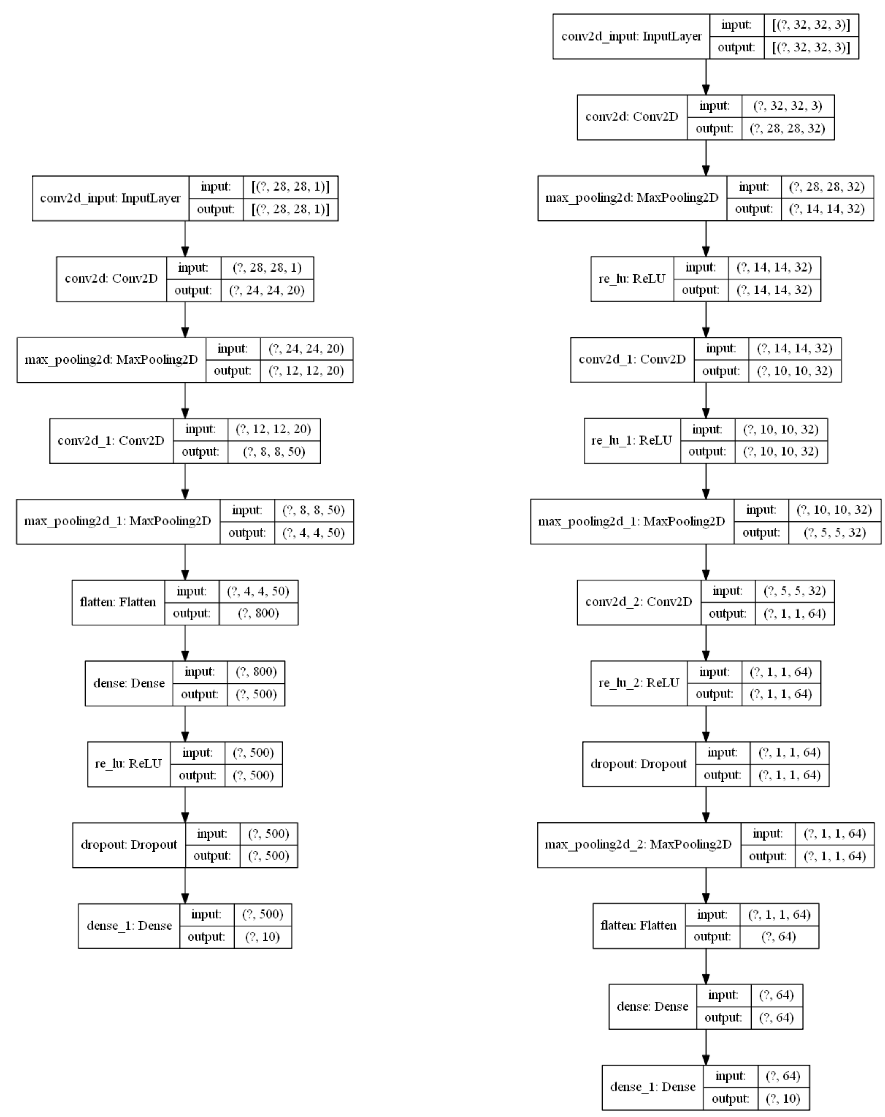
5. Dropout Estimation Simulations

In this section, an empirical study of the proposed CFAEE for a practical problem of dropout regularization in CNN is presented. A basic experimental setup (problem modeling, control parameter setup, and dataset details) is shown first, followed by a presentation of the obtained results, comparative analysis with other metaheuristics-based methods, and a discussion.

For experimental purposes, two CNN structures with default values provided by the Caffe library, which obtained modest performances for employed datasets, were used. The purpose of the experiment was to further investigate the performance of metaheuristics for optimizing dropout probability $dp$. The same experimental conditions as in [5] were utilized.

All metaheuristics, as well as the CNN framework, were developed in Python using its core and data science libraries (scikit-learn, NumPy, SciPy, along with pandas and matplotlib for visualization) and Keras API. Experiments are conducted on Intel^® CoreTM i7-8700K CPU, 64 GB RAM, and Windows 10 OS with 6 × NVIDIA GTX 1080 GPUs.

5.1. Basic Experimental Setup

The study proposed in this manuscript utilizes a similar research setup as shown in [5]. Four parameters that influence the CNN learning process, which were taken into consideration in this study, are: the learning rate $\eta$, L1 regularization (penalty, momentum) $\alpha$, L2 regularization (weight decay) $\lambda$, and the dropout probability $dp$. However, in all experiments, tuple ($\eta$, $\alpha$, $\lambda$) was fixed, while the metaheuristics approaches attempted to optimize only the $dp$ parameter. Therefore, this problem belongs to the group of global optimization challenges, with only one parameter that is being optimized.

In the conducted simulations, two CNN architectures, provided by the well-known Caffe library [66] examples (https://caffe.berkeleyvision.org/, accessed on 10 October 2021), as in [5], were utilized. First, CNN architecture was used for performing classification tasks for MNIST, Fashion-MNIST, Semeion, and USPS datasets, while the second was employed for CIFAR-10 challenge. The only differences in CNN design over the proposed Caffe CNNs are the following: an extra dropout layer was added, and for Semeion and USPS simulations, the kernel size was set to $3\times 3$ instead of $5\times 5$ (as provided in Caffe), due to the lower image resolutions.

Graphical representation of the utilized CNN structures generated by the plot_model Keras function is shown in Figure 4.

Method was tested on five well-known image classification datasets:

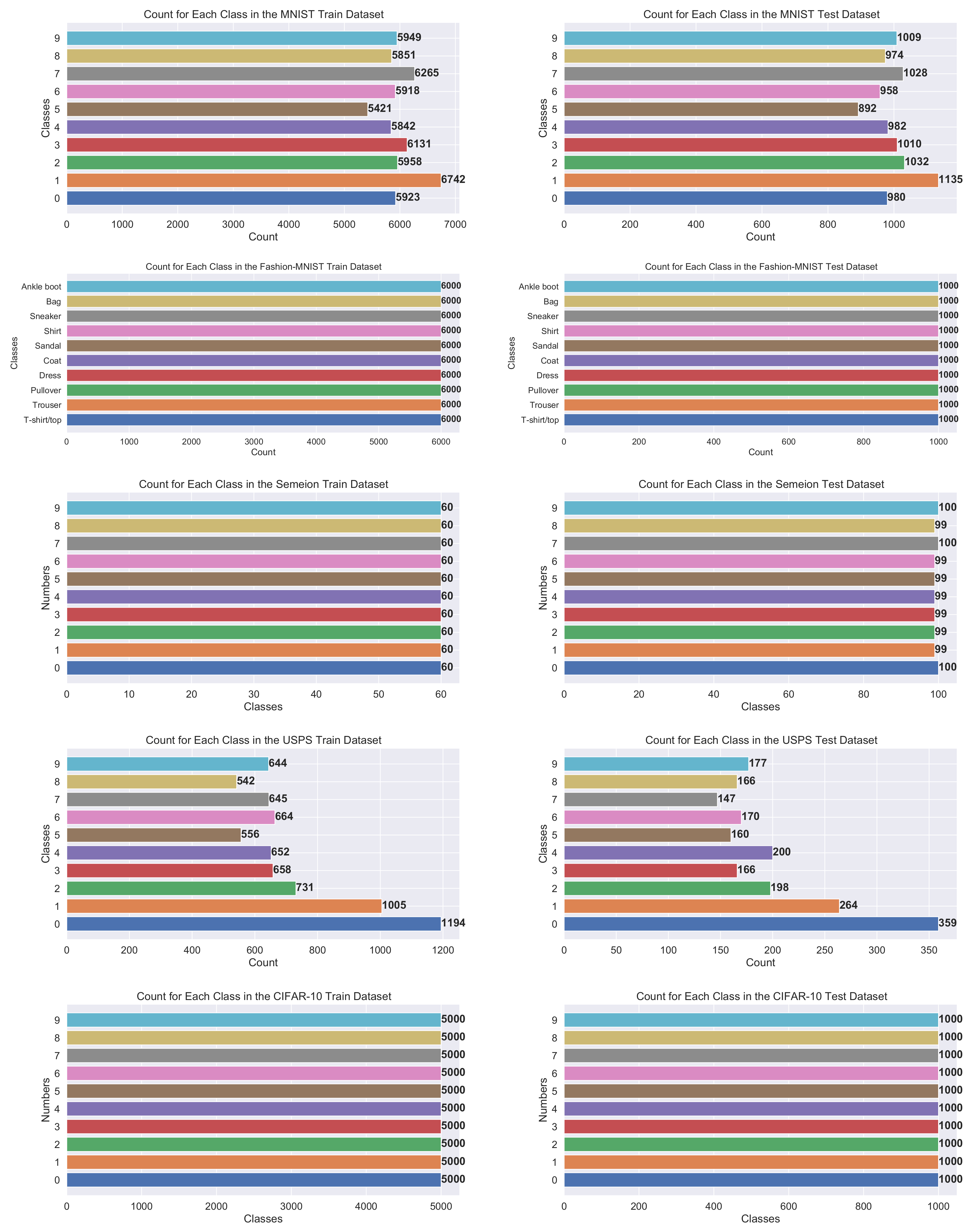
• MNIST—consists of images of handwritten digits “0–9”; it is divided into 60,000 training and 10,000 testing observations; image size $28\times 28$ pixels gray-scale (http://yann.lecun.com/exdb/mnist/, accessed on 10 October 2021);
• Fashion-MNIST—dataset of Zalando’s article images; it is comprised of different clothing images divided into 10 classes; it is split into 60,000 and 10,000 images used for training and testing, respectively; image size $28\times 28$ pixels (https://github.com/zalandoresearch/fashion-mnist, accessed on 10 October 2021);
• Semeion—includes a total of 1593 handwritten digits “0–9” images collected from 80 persons; digits are written accurately (normal way) and inaccurately (fast way); the original dataset is not split into training and testing; image size $16\times 16$ grayscale and each pixel is binarized (https://archive.ics.uci.edu/ml/datasets/Semeion+Handwritten+Digit, accessed on 10 October 2021);
• USPS—contains handwritten digits “0–9” images obtained from the envelopes of the United States Postal Service; dataset is split into 7291 training and 2007 testing images; image size $16\times 16$ gray-scale (http://statweb.stanford.edu/tibs/ElemStatLearn/datasets/zip.info.txt, accessed on 10 October 2021);
• CIFAR-10—consists of various images from 10 classes; subset of 80 million tiny images retrieved and collected by Alex Krizhevsky, Vinod Nair, and Geoffrey Hinton; divided into 50,000 images for training and 10,000 images for testing; image size $32\times 32$ color-scale (http://www.cs.toronto.edu/kriz/cifar.html, accessed on 10 October 2021).

The total number of instances per each class in the training and testing sets, for all datasets employed in the simulations, is shown in Figure 5. Nevertheless, some datasets are unbalanced (does not have the same number of observations for each class) in the original train and test sets; the original split was used in experiments and all metaheuristics were tested under the same experimental conditions. The only dataset that was not originally split into training and testing sets was Semeion; for the purpose of this study, it was manually divided into 400 and 993 observations used for training and testing, respectively, as suggested in [5].

The training set for each database was further divided into train and validation, while the same proportion of the number of instances for each class was maintained. Data preprocessing was not applied. The dataset details, in terms of the split, along with the training batch size (provided in parentheses), are shown in

Table 15. Datasets split into training, validation, and testing, along with the batch size.

Dataset	Train Set	Validation Set	Testing Set
MNIST	20.000 (64)	40.000 (100)	10.000 (100)
Fashion-MNIST	20.000 (64)	40.000 (100)	10.000 (100)
Semeion	200 (2)	400 (400)	993 (993)
USPS	2.406 (32)	4.885 (977)	2.007 (2.007)
CIFAR-10	20.000 (100)	30.000 (100)	10.000 (100)

. The same configuration was employed in [5].

The values for $\eta$, $\alpha$, and $\lambda$ parameters, as well as the number of training epochs, were set to default values, provided by the Caffe library with only an exception for the Semeion dataset. In this case, the $\eta$ was set to 0.001 (not Caffe default) due to fewer images in the dataset. The $dp$, which is subject to optimization, can take any continuous value from the range $[0,1]$. The parameter setup is summarized in

Table 16. Employed CNNs parameters summary.

Dataset	$\mathit{\eta }$	$\mathit{\alpha }$	$\mathit{\lambda }$	$\mathit{d}\mathit{p}$	Epochs
MNIST	0.01	0.9	0.0005	[0, 1]	10.000
Fashion-MNIST	0.01	0.9	0.0005	[0, 1]	10.000
Semeion	0.001	0,9	0.0005	[0, 1]	10.000
USPS	0.01	0.9	0.0005	[0, 1]	10.000
CIFAR-10	0.001	0.9	0.004	[0, 1]	4.000

.

Each solution in the population represents one possible $dp$ value. The fitness of solution is calculated in the following way: the CNN with $dp$ is generated and trained on the training set and validated on the validation set with early stopping conditions (the early stopping is adjusted as 5% of the total number of training epochs); afterwards, trained CNN is evaluated for the test set and classification error rate $E_r$ is return. The fitness is reversed, proportional to the $E_r$:$fit=1/E_r$.

All metaheuristics were tested with a total number of 77 $FFEs$.The sStudy proposed in [5] evaluated methods with $N=7$ and $T=10$, which also yielded a total of 77 $FFEs$ (7 + 7 × 10).

With the goal of visualizing the CNN dropout regularization experiment flow and design, the general CFAEE flowchart and the flowchart for fitness calculation are sown in Figure 6.

5.2. Results, Comparative Analysis, and Discussion

For the purpose of the study proposed in [5], the bat algorithm (BA) [67], cuckoo search (CS) [68], FA [1], and particle swarm optimization (PSO) [69] metaheuristics were implemented and tested. However, to compare the performance of metaheuristics-defined $dp$, results of the standard Caffe CNN with dropout (Dropout Caffe) and without dropout (Caffe) are also provided.

In the study proposed in this paper, all above metaheuristics were also implemented and tested to validate results provided in [5]. Additionally, besides the CFAEE method proposed in this manuscript, the following approaches were also included in the analysis: elephant herding optimization (EHO) [70], whale optimization algorithm (WOA) [53], sine cosine algorithm (SCA) [51], salp swarm algorithm (SSA), grasshopper optimization algorithm (GOA) [52], and biogeography-based optimization (BBO) [71].

The CFAEE was tested with the same control parameter adjustments as in bound-constrained experiments (Table 1). Summary of control parameters for other metaheuristics methods included in the analysis are summarized in

Table 17. Control parameter setup for metaheuristics included in the analysis.

Algorithm	Parameters
BA [67]	$f_{min}=0$, $f_{max}=2$, $A=0.5$, $r=0.5$
CS [68]	$\beta =1.5$, $p=0.25$, $\alpha =0.8$
PSO [69]	$c1=1.7$, $c2=1.7$, $\omega =0.7$
EHO [70]	$n{o}_{c}lan=5$, $\alpha =0.5$, $\beta =0.1$, $n{o}_{e}lite=2$
WOA [53]	$a_1$ linearly decreasing from 2 to 0, $a_2$ linearly decreasing from −1 to −2, b=1
SCA [51]	$a=2$, $r_1$ linearly decreasing from 2 to 0
SSA [72]	$c_1$ non-linearly decreasing from 2 to 0, $c2$ and $c3$ rand from [0, 1]
GOA [52]	c linearly decreasing from 1 to 0
BBO [71]	$hmp=1$, $imp=0.1$, $nbhk=2$
FA [1]	$\alpha =0.2$, ${\beta }_0=1.0$, $\gamma =1.0$

.

All metaheuristics methods were tested in 20 separate runs and the average reported accuracy was used as comparison metrics. Moreover, the mean obtained $dp$ value was also shown in the comparison table. Comparative analysis results are shown in

Table 18. Comparative results between the proposed CFAEE and other metaheuristics in terms of mean classification accuracy.

Method	MNIST		Fashion-MNIST		Semeion		USPS		CIFAR-10
	acc.	$\mathit{d}\mathit{p}$	acc.	$\mathit{d}\mathit{p}$	acc.	$\mathit{d}\mathit{p}$	acc.	$\mathit{d}\mathit{p}$	acc.	$\mathit{d}\mathit{p}$
Caffe	99.07	0	91.71	0	97.62	0	95.80	0	71.47	0
Dropout Caffe	99.18	0.5	92.53	0.5	98.14	0.5	96.21	0.5	72.08	0.5
BA	99.14	0.491	92.56	0.505	98.35	0.692	96.45	0.762	71.49	0.633
CS	99.14	0.489	92.41	0.491	98.21	0.544	96.31	0.715	71.21	0.669
PSO	99.16	0.493	92.38	0.481	97.79	0.371	96.33	0.725	71.51	0.621
EHO	99.13	0.475	92.36	0.470	98.11	0.481	96.24	0.682	71.15	0.705
WOA	99.15	0.489	92.43	0.493	98.23	0.561	96.32	0.722	71.23	0.685
SCA	99.17	0.496	92.53	0.501	98.25	0.580	96.29	0.705	71.54	0.597
SSA	99.19	0.499	92.63	0.527	98.31	0.642	96.41	0.753	71.58	0.529
GOA	99.16	0.492	92.44	0.494	98.15	0.513	96.15	0.481	70.95	0.849
BBO	99.13	0.474	92.35	0.468	98.16	0.515	96.17	0.483	71.08	0.768
FA	99.18	0.495	92.58	0.511	98.29	0.619	96.42	0.758	71.55	0.583
CFAEE	99.26	0.529	92.73	0.570	98.46	0.719	96.88	0.845	72.32	0.388

.

The results from Table 18 clearly indicate superior performance of the proposed CFAEE method regarding the $dp$ value that was subjected to the optimization process. On the MNIST dataset, the proposed CFAEE method obtained superior accuracy of 99.23% with the determined $dp$ value of 0.516. All other metaheuristics approaches obtained the $dp$ value below the standard Dropout Caffe value $dp=0.5$. In this particular case, the results obviously show that the $dp$ value should be slightly greater than 0.5 in order to achieve better accuracy, and the proposed CFAEE method was the only one that was able to achieve it.

A similar conclusion can be derived for the Fashion-MNIST experiment. Most methods included in the analysis generated $dp$, which is lower than 0.5, and worse results than those achieved by the Dropout Caffe were reported. However, BA, SSA SSA, FA, and the proposed CFAEE obtained better accuracy than Dropout Caffe with $dp>0.5$.

In the Semeion dataset, again, the proposed CFAEE obtained the best accuracy result of 98.46%, with the $dp$ value of 0.719. It is clear that the accuracy increases with the values of $dp$, higher than the standard Dropout Caffe value 0.5 in this particular dataset. The second best method was BA, which achieved an accuracy of 98.35% with $dp=0.692$. The simple Caffe that does not employ the dropout ($dp=0$) achieved 97.62% in this dataset, while the Dropout Caffe approach ($dp=0.5$) achieved an accuracy of 98.14%.

A similar pattern can be seen in the USPS dataset as well. The proposed CFAEE again achieved the best accuracy of 96.8% with the obtained $dp$ value of 0.845. Similar to the previous datasets, the increase of $dp$ value leads to better accuracy values. The second best method in this dataset was BA, which achieved 96.45 % with the $dp=0.762$. The improvement of the accuracy over the standard Caffe and Dropout Caffe methods is significant, as the proposed CFAEE achieved accuracy approximately 1% greater than the Caffe, and about 0.6% greater than the Dropout Caffe.

Finally, the results on the CIFAR-10 dataset show a different pattern, as they indicate that, if the $dp$ is larger than the standard Dropout Caffe ($dp=0.5$), the performance start to drop and accuracy decreases. In this particular case, the model drops out neurons, and it is not able to generalize well. At the same time, if the $dp$ is too small, again, the performances will drop (similar to the standard Caffe that utilizes $dp=0$). It can be concluded that, on the CIFAR-10 dataset, the best performances are achieved for the $dp$ values slightly below 0.5. The proposed CFAEE method achieved the best accuracy of 72.32% with the $dp=0.388$, and it was the only method that found the $dp$ value below 0.5, as all other metaheuristics determined the $dp$ values in range $[0.5,1]$.

Finally, the original FA method showed an average performance and the proposed CFAEE in all tests managed to substantially outscore its basic version. Therefore, similar to the case of unconstrained benchmarks, the improvements over the original approach were also validated against the practical challenge of dropout regularization.

Similarly, as it was performed for unconstrained benchmark problem set 1 (Section 4.2), to establish if there were significant result differences between the proposed CFAEE and other methods, a Wilcoxon signed rank-test was conducted. A mean classification error rate generated over 20 independent runs and critical level $\alpha =0.05$ were taken for the test.

Results of the Wilcoxon signed-rank test are shown in

Table 19. Statistical comparison of classification error rate metrics obtained by CFAEE for CNN experiments, with other approaches by Wilcoxon Signed-Rank Test at $\alpha$ = 0.05.

Function	CFAEE	Caffe	DropoutCaffe	BA	CS	PSO	EHO	WOA	SCA	SSA	GOA	BBO	FA
MNIST	0.74	0.9	0.82	0.86	0.86	0.8	0.87	0.85	0.83	0.81	0.84	0.87	0.82
Fashion-MNIST	7.27	8.29	7.47	7.44	7.59	7.62	7.64	7.57	7.47	7.37	7.56	7.65	7.42
Semeion	1.54	2.38	1.86	1.65	1.79	2.21	1.89	1.77	1.75	1.69	1.85	1.84	1.71
USPS	3.12	4.2	3.79	3.55	3.69	3.67	3.76	3.68	3.71	3.59	3.85	3.83	3.58
CIFAR-10	27.68	28.53	27.92	28.51	28.79	28.5	28.85	28.77	28.46	28.42	29.05	28.92	28.45
p-value	3.125$\times {10}^{-2}$	3.125$\times {10}^{-2}$	3.125$\times {10}^{-2}$	3.125$\times {10}^{-2}$	3.125$\times {10}^{-2}$	3.125$\times {10}^{-2}$	3.125$\times {10}^{-2}$	3.125$\times {10}^{-2}$	3.125$\times {10}^{-2}$	3.125$\times {10}^{-2}$	3.125$\times {10}^{-2}$	3.125$\times {10}^{-2}$	3.125$\times {10}^{-2}$

. The calculated p-values in all cases are lesser than critical values $\alpha =0.05$, which implies that the proposed CFAEE, on average, substantially outperformed all other approaches.

6. Conclusions

The proposed manuscript introduced a novel FA approach that further enhanced both exploration and exploitation processes of the original method. The CFAEE incorporates an explicit exploration mechanism and CLS, and in this way, the observed deficiencies of the original FA were suppressed.

Following the recent practices in the optimization process—the introduced CFAEE algorithm was first tested on the recent CEC benchmark functions set, and the obtained results were compared with other modern metaheuristic methods, which were tested under the same experimental environment. Additionally, the statistical tests were executed and delivered the proofs that the enhanced FA algorithm outscored other methods, significantly. Furthermore, the proposed CFAEE outperforms the original FA.

The second part of the experiment focused on applying the proposed CFAEE to the practical CNN problem-optimization of the dropout probability value. Dropout is crucial in overfitting prevention, and it is an important challenge in the machine learning domain. The CFAEE driven CNN was tested on five standard datasets: MNIST, Fashion-MNIST, Semeion, USPS, and CIFAR-10. Furthermore, since the potential of metaheuristics for this type of challenge was not investigated enough, 10 other well-known swarm intelligence approaches were also implemented and tested for this problem. The achieved accuracies on those datasets indicate that the CFAEE has superior performance over other methods, as well as a promising future in this area.

Accordingly, future work will focus on applying the proposed CFAEE method on other machine learning problems. Due to its promising performances, CFAEE will be adapted and used in tackling other NP-hard problems, including challenges in wireless sensor networks and cloud computing. Finally, regularization in CNNs can be further addressed by utilizing CFAEE and fine-tuning $\alpha$ and $\lambda$ parameters, with a goal to obtain even better classification accuracy. Moreover, the variables of the convolutional layers, such as the size and depth of the filters, can be parameterized through the CFAEE, instead of the more classical metaheuristic algorithms [73].

References

1. Yang, X.S. Firefly Algorithms for Multimodal Optimization. In Stochastic Algorithms: Foundations and Applications; Watanabe, O., Zeugmann, T., Eds.; Springer: Berlin/Heidelberg, Germany, 2009; pp. 169–178. [Google Scholar]
2. Bezdan, T.; Cvetnic, D.; Gajic, L.; Zivkovic, M.; Strumberger, I.; Bacanin, N. Feature Selection by Firefly Algorithm with Improved Initialization Strategy. In Proceedings of the 7th Conference on the Engineering of Computer Based Systems, Novi Sad, Serbia, 26–27 May 2021; pp. 1–8. [Google Scholar]
3. Bacanin, N.; Bezdan, T.; Venkatachalam, K.; Al-Turjman, F. Optimized convolutional neural network by firefly algorithm for magnetic resonance image classification of glioma brain tumor grade. J. Real Time Image Process. 2021, 18, 1085–1098. [Google Scholar] [CrossRef]
4. Kumar, V.; Kumar, D. A systematic review on firefly algorithm: Past, present, and future. Arch. Comput. Methods Eng. 2021, 28, 3269–3291. [Google Scholar] [CrossRef]
5. de Rosa, G.; Papa, J.; Yang, X.S. Handling Dropout Probability Estimation in Convolution Neural Networks Using Metaheuristics. Soft Comput. 2018, 22, 6147–6156. [Google Scholar] [CrossRef] [Green Version]
6. Zivkovic, M.; Bacanin, N.; Venkatachalam, K.; Nayyar, A.; Djordjevic, A.; Strumberger, I.; Al-Turjman, F. COVID-19 cases prediction by using hybrid machine learning and beetle antennae search approach. Sustain. Cities Soc. 2021, 66, 102669. [Google Scholar] [CrossRef] [PubMed]
7. Wainer, J.; Fonseca, P. How to tune the RBF SVM hyperparameters? An empirical evaluation of 18 search algorithms. Artif. Intell. Rev. 2021, 54, 4771–4797. [Google Scholar] [CrossRef]
8. Basha, J.; Bacanin, N.; Vukobrat, N.; Zivkovic, M.; Venkatachalam, K.; Hubálovskỳ, S.; Trojovskỳ, P. Chaotic Harris Hawks Optimization with Quasi-Reflection-Based Learning: An Application to Enhance CNN Design. Sensors 2021, 21, 6654. [Google Scholar] [CrossRef]
9. Beni, G. Swarm intelligence. Complex Soc. Behav. Syst. Game Theory Agent Based Model. 2020, 791–818. [Google Scholar] [CrossRef]
10. Abraham, A.; Guo, H.; Liu, H. Swarm intelligence: Foundations, perspectives and applications. In Swarm Intelligent Systems; Springer: Berlin/Heidelberg, Germany, 2006; pp. 3–25. [Google Scholar]
11. Li, M.W.; Wang, Y.T.; Geng, J.; Hong, W.C. Chaos cloud quantum bat hybrid optimization algorithm. Nonlinear Dyn. 2021, 103, 1167–1193. [Google Scholar] [CrossRef]
12. Zivkovic, M.; Bacanin, N.; Tuba, E.; Strumberger, I.; Bezdan, T.; Tuba, M. Wireless Sensor Networks Life Time Optimization Based on the Improved Firefly Algorithm. In Proceedings of the 2020 International Wireless Communications and Mobile Computing (IWCMC), Limassol, Cyprus, 15–19 June 2020; pp. 1176–1181. [Google Scholar]
13. Zivkovic, M.; Bacanin, N.; Zivkovic, T.; Strumberger, I.; Tuba, E.; Tuba, M. Enhanced Grey Wolf Algorithm for Energy Efficient Wireless Sensor Networks. In Proceedings of the 2020 Zooming Innovation in Consumer Technologies Conference (ZINC), Online, 26–27 May 2020; pp. 87–92. [Google Scholar]
14. Bacanin, N.; Tuba, E.; Zivkovic, M.; Strumberger, I.; Tuba, M. Whale Optimization Algorithm with Exploratory Move for Wireless Sensor Networks Localization. In Proceedings of the International Conference on Hybrid Intelligent Systems, Sehore, India, 10–12 December 2019; Springer: Berlin/Heidelberg, Germany, 2019; pp. 328–338. [Google Scholar]
15. Zivkovic, M.; Zivkovic, T.; Venkatachalam, K.; Bacanin, N. Enhanced Dragonfly Algorithm Adapted for Wireless Sensor Network Lifetime Optimization. In Data Intelligence and Cognitive Informatics; Springer: Berlin/Heidelberg, Germany, 2021; pp. 803–817. [Google Scholar]
16. Bacanin, N.; Bezdan, T.; Tuba, E.; Strumberger, I.; Tuba, M.; Zivkovic, M. Task scheduling in cloud computing environment by grey wolf optimizer. In Proceedings of the 2019 27th Telecommunications Forum (TELFOR), Belgrade, Serbia, 26–27 November 2019; pp. 1–4. [Google Scholar]
17. Strumberger, I.; Bacanin, N.; Tuba, M.; Tuba, E. Resource scheduling in cloud computing based on a hybridized whale optimization algorithm. Appl. Sci. 2019, 9, 4893. [Google Scholar] [CrossRef] [Green Version]
18. Bezdan, T.; Zivkovic, M.; Tuba, E.; Strumberger, I.; Bacanin, N.; Tuba, M. Glioma Brain Tumor Grade Classification from MRI Using Convolutional Neural Networks Designed by Modified FA. In Proceedings of the International Conference on Intelligent and Fuzzy Systems, Istanbul, Turkey, 21–23 July 2020; Springer: Berlin/Heidelberg, Germany, 2020; pp. 955–963. [Google Scholar]
19. Bacanin, N.; Bezdan, T.; Tuba, E.; Strumberger, I.; Tuba, M. Monarch butterfly optimization based convolutional neural network design. Mathematics 2020, 8, 936. [Google Scholar] [CrossRef]
20. Zivkovic, M.; Venkatachalam, K.; Bacanin, N.; Djordjevic, A.; Antonijevic, M.; Strumberger, I.; Rashid, T.A. Hybrid Genetic Algorithm and Machine Learning Method for COVID-19 Cases Prediction. In Proceedings of the International Conference on Sustainable Expert Systems: ICSES 2020, Nepal, South Asia, 17–18 September 2020; Springer: Berlin/Heidelberg, Germany, 2021; Volume 176, p. 169. [Google Scholar]
21. Milosevic, S.; Bezdan, T.; Zivkovic, M.; Bacanin, N.; Strumberger, I.; Tuba, M. Feed-Forward Neural Network Training by Hybrid Bat Algorithm. In Proceedings of the Modelling and Development of Intelligent Systems: 7th International Conference, MDIS 2020, Sibiu, Romania, 22–24 October 2020; Revised Selected Papers 7. Springer: Berlin/Heidelberg, Germany, 2021; pp. 52–66. [Google Scholar]
22. Gajic, L.; Cvetnic, D.; Zivkovic, M.; Bezdan, T.; Bacanin, N.; Milosevic, S. Multi-layer Perceptron Training Using Hybridized Bat Algorithm. In Computational Vision and Bio-Inspired Computing; Springer: Berlin/Heidelberg, Germany, 2021; pp. 689–705. [Google Scholar]
23. Hongtao, L.; Qinchuan, Z. Applications of deep convolutional neural network in computer vision. J. Data Acquis. Process. 2016, 31, 1–17. [Google Scholar]
24. Xiao, T.; Xu, Y.; Yang, K.; Zhang, J.; Peng, Y.; Zhang, Z. The application of two-level attention models in deep convolutional neural network for fine-grained image classification. In Proceedings of the IEEE Conference on Computer Vision and Pattern Recognition, Boston, MA, USA, 7–12 June 2015; pp. 842–850. [Google Scholar]
25. Zhang, Y.; Zhao, D.; Sun, J.; Zou, G.; Li, W. Adaptive convolutional neural network and its application in face recognition. Neural Process. Lett. 2016, 43, 389–399. [Google Scholar] [CrossRef]
26. Lawrence, S.; Giles, C.L.; Tsoi, A.C.; Back, A.D. Face recognition: A convolutional neural-network approach. IEEE Trans. Neural Netw. 1997, 8, 98–113. [Google Scholar] [CrossRef] [Green Version]
27. Ranjan, R.; Sankaranarayanan, S.; Castillo, C.D.; Chellappa, R. An all-in-one convolutional neural network for face analysis. In Proceedings of the 2017 12th IEEE International Conference on Automatic Face & Gesture Recognition (FG 2017), Washington, DC, USA, 30 May–3 June 2017; pp. 17–24. [Google Scholar]
28. Matsugu, M.; Mori, K.; Mitari, Y.; Kaneda, Y. Subject independent facial expression recognition with robust face detection using a convolutional neural network. Neural Netw. 2003, 16, 555–559. [Google Scholar] [CrossRef]
29. Ramaiah, N.P.; Ijjina, E.P.; Mohan, C.K. Illumination invariant face recognition using convolutional neural networks. In Proceedings of the 2015 IEEE International Conference on Signal Processing, Informatics, Communication and Energy Systems (SPICES), Kozhikode, India, 19–21 February 2015; pp. 1–4. [Google Scholar]
30. Simard, P.Y.; Steinkraus, D.; Platt, J.C. Best practices for convolutional neural networks applied to visual document analysis. In Proceedings of the ICDAR, Edinburgh, UK, 3–6 August 2003; Volume 3. [Google Scholar]
31. Afzal, M.Z.; Capobianco, S.; Malik, M.I.; Marinai, S.; Breuel, T.M.; Dengel, A.; Liwicki, M. Deepdocclassifier: Document classification with deep convolutional neural network. In Proceedings of the 2015 13th International Conference on Document Analysis and Recognition (ICDAR), Tunis, Tunisia, 23–26 August 2015; pp. 1111–1115. [Google Scholar]
32. Stoean, C.; Lichtblau, D. Author Identification Using Chaos Game Representation and Deep Learning. Mathematics 2020, 8, 1933. [Google Scholar] [CrossRef]
33. Špetlík, R.; Franc, V.; Matas, J. Visual heart rate estimation with convolutional neural network. In Proceedings of the British Machine Vision Conference, Newcastle, UK, 3–6 September 2018; pp. 3–6. [Google Scholar]
34. Li, Q.; Cai, W.; Wang, X.; Zhou, Y.; Feng, D.D.; Chen, M. Medical image classification with convolutional neural network. In Proceedings of the 2014 13th International Conference on Control Automation Robotics & Vision (ICARCV), Singapore, 10–12 December 2014; pp. 844–848. [Google Scholar]
35. Ting, F.F.; Tan, Y.J.; Sim, K.S. Convolutional neural network improvement for breast cancer classification. Expert Syst. Appl. 2019, 120, 103–115. [Google Scholar] [CrossRef]
36. Liu, Y.; Racah, E.; Correa, J.; Khosrowshahi, A.; Lavers, D.; Kunkel, K.; Wehner, M.; Collins, W. Application of deep convolutional neural networks for detecting extreme weather in climate datasets. arXiv 2016, arXiv:1605.01156. [Google Scholar]
37. Chattopadhyay, A.; Hassanzadeh, P.; Pasha, S. Predicting clustered weather patterns: A test case for applications of convolutional neural networks to spatio-temporal climate data. Sci. Rep. 2020, 10, 1317. [Google Scholar] [CrossRef]
38. Yang, X.S.; Xingshi, H. Firefly Algorithm: Recent Advances and Applications. Int. J. Swarm Intell. 2013, 1, 36–50. [Google Scholar] [CrossRef] [Green Version]
39. Strumberger, I.; Tuba, E.; Bacanin, N.; Zivkovic, M.; Beko, M.; Tuba, M. Designing convolutional neural network architecture by the firefly algorithm. In Proceedings of the 2019 International Young Engineers Forum (YEF-ECE), Caparica, Portugal, 10 May 2019; pp. 59–65. [Google Scholar]
40. Strumberger, I.; Bacanin, N.; Tuba, M. Enhanced Firefly Algorithm for Constrained Numerical Optimization, IEEE Congress on Evolutionary Computation. In Proceedings of the IEEE International Congress on Evolutionary Computation (CEC 2017), Donostia, Spain, 5–8 June 2017; pp. 2120–2127. [Google Scholar]
41. Xu, G.H.; Zhang, T.W.; Lai, Q. A new firefly algorithm with mean condition partial attraction. Appl. Intell. 2021, 1–14. [Google Scholar] [CrossRef]
42. Bacanin, N.; Tuba, M. Firefly Algorithm for Cardinality Constrained Mean-Variance Portfolio Optimization Problem with Entropy Diversity Constraint. Sci. World J. Spec. Issue Comput. Intell. Metaheuristic Algorithms Appl. 2014, 2014, 721521. [Google Scholar] [CrossRef] [PubMed]
43. Wang, H.; Zhou, X.; Sun, H.; Yu, X.; Zhao, J.; Zhang, H.; Cui, L. Firefly algorithm with adaptive control parameters. Soft Comput. 2017, 3, 5091–5102. [Google Scholar] [CrossRef]
44. Karaboga, D.; Basturk, B. On the performance of artificial bee colony (ABC) algorithm. Appl. Soft Comput. 2008, 8, 687–697. [Google Scholar] [CrossRef]
45. Moradi, P.; Imanian, N.; Qader, N.N.; Jalili, M. Improving exploration property of velocity-based artificial bee colony algorithm using chaotic systems. Inf. Sci. 2018, 465, 130–143. [Google Scholar] [CrossRef]
46. Alatas, B. Chaotic bee colony algorithms for global numerical optimization. Expert Syst. Appl. 2010, 37, 5682–5687. [Google Scholar] [CrossRef]
47. dos Santos Coelho, L.; Mariani, V.C. Use of chaotic sequences in a biologically inspired algorithm for engineering design optimization. Expert Syst. Appl. 2008, 34, 1905–1913. [Google Scholar] [CrossRef]
48. Li, C.; Zhou, J.; Xiao, J.; Xiao, H. Parameters identification of chaotic system by chaotic gravitational search algorithm. Chaos Solitons Fractals 2012, 45, 539–547. [Google Scholar] [CrossRef]
49. Chen, H.; Xu, Y.; Wang, M.; Zhao, X. A balanced whale optimization algorithm for constrained engineering design problems. Appl. Math. Model. 2019, 71, 45–59. [Google Scholar] [CrossRef]
50. Liang, X.; Cai, Z.; Wang, M.; Zhao, X.; Chen, H.; Li, C. Chaotic oppositional sine–cosine method for solving global optimization problems. Eng. Comput. 2020, 1–17. [Google Scholar] [CrossRef]
51. Mirjalili, S. SCA: A sine cosine algorithm for solving optimization problems. Knowl. Based Syst. 2016, 96, 120–133. [Google Scholar] [CrossRef]
52. Mirjalili, S.Z.; Mirjalili, S.; Saremi, S.; Faris, H.; Aljarah, I. Grasshopper optimization algorithm for multi-objective optimization problems. Appl. Intell. 2018, 48, 805–820. [Google Scholar] [CrossRef]
53. Mirjalili, S.; Lewis, A. The whale optimization algorithm. Adv. Eng. Softw. 2016, 95, 51–67. [Google Scholar] [CrossRef]
54. Liu, J.; Mao, Y.; Liu, X.; Li, Y. A dynamic adaptive firefly algorithm with globally orientation. Math. Comput. Simul. 2020, 174, 76–101. [Google Scholar] [CrossRef]
55. Zhu, Q.; Xiao, Y.; Chen, W.; Ni, C.; Chen, Y. Research on the improved mobile robot localization approach based on firefly algorithm. Chin. J. Sci. Instrum. 2016, 37, 323–329. [Google Scholar]
56. Kaveh, A.; Javadi, S. Chaos-based firefly algorithms for optimization of cyclically large-size braced steel domes with multiple frequency constraints. Comput. Struct. 2019, 214, 28–39. [Google Scholar] [CrossRef]
57. Yang, X.S. Firefly Algorithm, Lévy Flights and Global Optimization. In Research and Development in Intelligent Systems XXVI; Bramer, M., Ellis, R., Petridis, M., Eds.; Springer: London, UK, 2010; pp. 209–218. [Google Scholar]
58. Yu, S.; Zhu, S.; Ma, Y.; Mao, D. A variable step size firefly algorithm for numerical optimization. Appl. Math. Comput. 2015, 263, 214–220. [Google Scholar] [CrossRef]
59. Awad, N.; Ali, M.; Liang, J.; Qu, B.; Suganthan, P.; Definitions, P. Evaluation criteria for the CEC 2017 special session and competition on single objective real-parameter numerical optimization. Technol. Rep. 2016. Available online: http://home.elka.pw.edu.pl/ (accessed on 4 October 2021).
60. Gupta, S.; Deep, K. Improved sine cosine algorithm with crossover scheme for global optimization. Knowl. Based Syst. 2019, 165, 374–406. [Google Scholar] [CrossRef]
61. Hussien, A.G.; Amin, M. A self-adaptive Harris Hawks optimization algorithm with opposition-based learning and chaotic local search strategy for global optimization and feature selection. Int. J. Mach. Learn. Cybern. 2021, 1–28. [Google Scholar] [CrossRef]
62. Friedman, M. The use of ranks to avoid the assumption of normality implicit in the analysis of variance. J. Am. Stat. Assoc. 1937, 32, 675–701. [Google Scholar] [CrossRef]
63. Friedman, M. A comparison of alternative tests of significance for the problem of m rankings. Ann. Math. Stat. 1940, 11, 86–92. [Google Scholar] [CrossRef]
64. Iman, R.L.; Davenport, J.M. Approximations of the critical region of the fbietkan statistic. Commun. Stat. Theory Methods 1980, 9, 571–595. [Google Scholar] [CrossRef]
65. Sheskin, D.J. Handbook of Parametric and Nonparametric Statistical Procedures; Chapman and Hall/CRC: Boca Raton, FL, USA, 2020. [Google Scholar]
66. Jia, Y.; Shelhamer, E.; Donahue, J.; Karayev, S.; Long, J.; Girshick, R.; Guadarrama, S.; Darrell, T. Caffe: Convolutional architecture for fast feature embedding. In Proceedings of the 22nd ACM International Conference on Multimedia, Orlando, FL, USA, 3–7 November 2014; pp. 675–678. [Google Scholar]
67. Yang, X.S.; Hossein Gandomi, A. Bat algorithm: A novel approach for global engineering optimization. Eng. Comput. 2012, 29, 464–483. [Google Scholar] [CrossRef] [Green Version]
68. Gandomi, A.H.; Yang, X.S.; Alavi, A.H. Cuckoo search algorithm: A metaheuristic approach to solve structural optimization problems. Eng. Comput. 2013, 29, 17–35. [Google Scholar] [CrossRef]
69. Kennedy, J.; Eberhart, R. Particle swarm optimization. In Proceedings of the ICNN’95-International Conference on Neural Networks, Perth, Australia, 27 November–1 December 1995; Volume 4, pp. 1942–1948. [Google Scholar]
70. Wang, G.G.; Deb, S.; Gao, X.Z.; Coelho, L.D.S. A new metaheuristic optimisation algorithm motivated by elephant herding behaviour. Int. J. Bio-Inspired Comput. 2016, 8, 394–409. [Google Scholar] [CrossRef]
71. Simon, D. Biogeography-based optimization. IEEE Trans. Evol. Comput. 2008, 12, 702–713. [Google Scholar] [CrossRef] [Green Version]
72. Mirjalili, S.; Gandomi, A.H.; Mirjalili, S.Z.; Saremi, S.; Faris, H.; Mirjalili, S.M. Salp Swarm Algorithm: A bio-inspired optimizer for engineering design problems. Adv. Eng. Softw. 2017, 114, 163–191. [Google Scholar] [CrossRef]
73. Stoean, R. Analysis on the potential of an EA–surrogate modelling tandem for deep learning parametrization: An example for cancer classification from medical images. Neural Comput. Appl. 2018, 32, 313–322. [Google Scholar] [CrossRef]
Figure 1. Mean convergence speed graphs for some benchmark instances (Benchmark set 1).
Mathematics 09 02705 g001
Figure 2. Dispersion of best results over runs for functions F4, F5, F7, F9, F10, F12 (Benchmark set 2).
Mathematics 09 02705 g002
Figure 3. Dispersion of best results over runs for functions F15, F18, F20, F22, F26, F30 (Benchmark set 2).
Mathematics 09 02705 g003
Figure 4. Example instance of MNIST/Fashion-MNIST/Semeion/USPS models (left) and example instance of CIFAR-10 model (right).
Mathematics 09 02705 g004
Figure 5. Number of instances per each class in the training and testing sets for MNIST, Fashion-MNIST, Semeion, USPS, and CIFAR-10 datasets.
Mathematics 09 02705 g005
Figure 6. (a) General CFAEE flowchart (left); (b) flowchart for fitness calculation (right).
Mathematics 09 02705 g006