Reinforcement Learning Approaches to Optimal Market Making

Abstract

Market making is the process whereby a market participant, called a market maker, simultaneously and repeatedly posts limit orders on both sides of the limit order book of a security in order to both provide liquidity and generate profit. Optimal market making entails dynamic adjustment of bid and ask prices in response to the market maker’s current inventory level and market conditions with the goal of maximizing a risk-adjusted return measure. This problem is naturally framed as a Markov decision process, a discrete-time stochastic (inventory) control process. Reinforcement learning, a class of techniques based on learning from observations and used for solving Markov decision processes, lends itself particularly well to it. Recent years have seen a very strong uptick in the popularity of such techniques in the field, fueled in part by a series of successes of deep reinforcement learning in other domains. The primary goal of this paper is to provide a comprehensive and up-to-date overview of the current state-of-the-art applications of (deep) reinforcement learning focused on optimal market making. The analysis indicated that reinforcement learning techniques provide superior performance in terms of the risk-adjusted return over more standard market making strategies, typically derived from analytical models.

1. Introduction

Modern financial markets are increasingly order-driven and electronic, with the electronic limit order book (LOB) becoming the dominant trading form for multiple asset classes. This electronification of financial markets has led to the increased importance of certain (algorithmic) trading strategies, in particular market making strategies.

Market making (MM) is the process whereby a market participant simultaneously and repeatedly posts limit orders on both sides of the limit order book of a given security, with the goal of capturing the difference between their prices, known as the quoted spread. A limit order book (LOB) is simply a collection of outstanding offers to buy or sell (limit orders). Traders that rely on MM strategies are simply referred to as market makers. A market maker might, for example, post a buy limit order at USD 99 and a sell limit order at USD 101. If both orders become executed (i.e., if both a counterparty willing to sell at USD 99 and a counterparty willing to buy at USD 101 emerge), the market maker will capture the spread, i.e., earn USD 2, all while providing the market with liquidity. However, if only one of the limit orders becomes executed, the market maker will not only fail to capture the spread, but also obtain a nonzero inventory and consequently take on the inventory risk that stems from fluctuations in the market value of the held asset. A risk-averse market maker hence adjusts its quotes to increase the probability of selling when its inventory is strictly positive, and vice versa, in order to dispose of the inventory and mitigate the associated risk.

Market makers act to maximize their risk-adjusted returns while at the same time playing a key role in the market by providing it with liquidity. Optimal MM entails dynamic adjustment of bid and ask prices in response to the market maker’s current inventory level, current market conditions, and potentially additional variables. It is a salient and well-studied problem in the field of quantitative finance, as well as a topic of immense interest to both institutional (banks, large-scale companies) and individual investors (such as private stock or cryptocurrency traders). Due to engaging in the MM mechanism, market makers are exposed to multiple risks, including not only the inventory and execution, but also adverse selection, latency, and model uncertainty risks. Most of the research in the field focuses on the inventory risk and, to a somewhat lesser extent, the adverse selection risk. Due to the need for inventory control, MM is naturally framed as a Markov decision process (MDP), a discrete-time stochastic control process. Under such a formulation, the market maker acts at discrete time steps by selecting prices at which to post limit orders, and this selection constitutes a control mechanism.

Analytical approaches to MM abound in the literature. Arguably the most prominent such approach was provided by Avellaneda and Stoikov [1], who introduced a novel analytical MM model, the Avellaneda–Stoikov (AS) model, and used the underlying Hamilton–Jacobi–Bellman (HJB) equations to derive closed-form approximations to the optimal quotes of a market maker. Most analytical approaches follow a similar recipe, deriving (near-)optimal strategies via the use of a system of differential equations underpinning the assumed model. However, such models (1) are typically predicated upon a set of strong, naive assumptions, (2) employ multiple parameters that need to be laboriously calibrated on historical market data, and (3) fail to properly take into account the market microstructure dynamics, especially by assuming inconsistent limit order book models [2]. For example, the AS model assumes that the reference price follows a driftless diffusion process, that the intensities at which the market maker’s limit orders become filled only depend on the distance from the reference price, and that the order arrivals and the reference price are completely independent, all of which are proven not to be reliable assumptions. Despite differing with respect to many facets, such as the choice of the objective function and other modeling details, approaches belonging to this category tend to be ill-suited for real-world MM modeling. Hence, there is a glaring need for novel, more robust, data-driven approaches, ideally even capable of learning directly from data in a model-free fashion.

Reinforcement learning (RL) is a class of machine learning techniques for direct adaptive control. It comprises various data-driven approaches for efficiently solving MDPs from observations and, as such, lends itself particularly well to the problem of optimal MM. Lately, the popularity of deep reinforcement learning (DRL), the combination of RL and deep learning (DL) in which deep neural networks (DNNs) are used as function approximators for the RL state–action value function and/or policy, has grown immensely due to a series of outstanding successes in various complex sequential decision-making tasks, including the game of Go [3], continuous robotic control [4], and autonomous driving [5].

Partly fueled by this, recent years (especially from 2018 onwards) have witnessed a very strong uptick in the popularity of RL, and especially DRL approaches in the field. This surge of interest is far from being confined to the topic of optimal MM. Au contraire, (D)RL applications in finance are numerous and include, for example, portfolio optimization [6], options pricing [7], and optimal execution [8], a research area intimately related to optimal MM, with multiple researchers working across both areas. Whereas numerous reviews on the applications of (D)RL in finance and economics [9,10] exist, to the authors’ knowledge, no review studies have been published on the topic of optimal market making. Therefore, our goal is to provide a comprehensive and up-to-date overview of the current state-of-the-art applications of (D)RL directly focused on optimal MM. Our analysis indicates that (D)RL approaches provide superior performance in terms of the risk-adjusted return over more standard MM strategies, mostly derived from analytical models based on simple heuristics. Furthermore, we provide a convenient categorization of such approaches, analyze multiple facets of RL frameworks proposed therein, and finally, shed some light on what we identify as viable future research directions.

This paper is organized as follows: Section 2 gives an overview of the MDP, a mathematical framework for modeling sequential decision-making problems. Furthermore, it delves into various classes of RL algorithms, particularly covering dynamic programming, temporal difference, policy gradient, and actor–critic methods. Section 3 provides a categorized overview of the current state-of-the-art applications of RL in optimal MM and expounds on their characteristics, advantages, and disadvantages, while Section 4 provides a thorough statistical analysis of the literature, covering multiple aspects, including the state and action space representation, the reward function formulation, and the use of function approximation. Lastly, Section 5 wraps up the paper by considering some potentially promising future research directions.

2. Overview of Reinforcement Learning

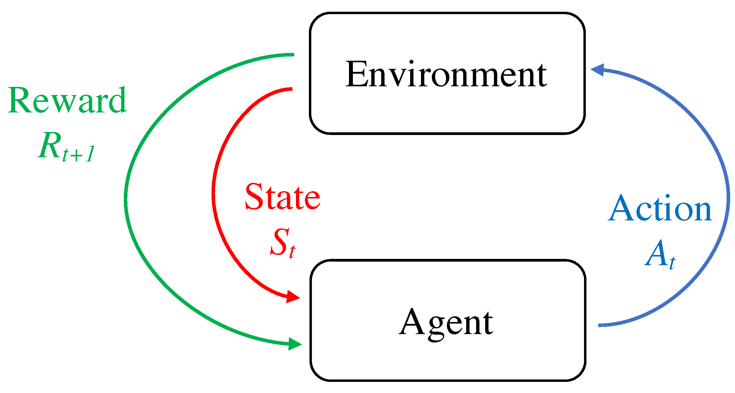
2.1. Markov Decision Process

A Markov decision process (MDP) is a stochastic control process, usually considered in discrete time, as shown in Figure 1. Formally [11], an MDP is a tuple $(\mathcal{S},\mathcal{A},\mathcal{P},\mathcal{R},\gamma )$ with:

• $\mathcal{S}$— a set of states;
• $\mathcal{A}$—a set of actions;
• $\mathcal{P}:\mathcal{S}\times \mathcal{A}\times \mathcal{S}\mapsto [0,1]$—a transition probability function (often expressed as a three-dimensional matrix);
• $\mathcal{R}:\mathcal{S}\times \mathcal{A}\mapsto \mathbb{R}$—a reward function;
• $\gamma \in [0,1]$—a discount factor, capturing a possible preference for earlier rewards.

At each discrete time t, the decision-maker, referred to as the agent, observes the current state of the environment $S_t$ and uses this information to select the action $A_t$, which then affects the next state of the environment $S_{t+1}$ and the reward $R_{t+1}$. This process is then iterated, and a (possibly infinite) sequence of states, actions, and rewards $(S_0,A_0,R_1,\dots ,S_t,A_t,R_{t+1},\dots )$ is obtained. The environment is typically defined as everything outside the agent’s direct control. Note that the action $A_t$ generally does not uniquely determine $S_{t+1}$: the transition matrix can be stochastic. Remarkably, the next state $S_{t+1}$ depends only on $S_t$ and $A_t$ and is therefore conditionally independent of past states and actions, given the current state–action. Therefore, the state transitions of an MDP meet the Markov property [12], thus warranting its name.

The agent’s selection of actions, i.e., its strategy is modeled as a function called a policy. A policy can be either stochastic or deterministic. A stochastic policy $\pi :\mathcal{A}\times \mathcal{S}\to [0,1]$ gives the probability of choosing action $A_t=a$ given state $S_t=s$. A deterministic policy $\pi :\mathcal{S}\to \mathcal{A}$ directly maps states into actions.

The goal of the agent is to maximize the expected discounted cumulative rewards (also called the return), formally given by the following expression:

$$G_t=R_{t+1}+\gamma R_{t+2}+\dots =\sum _{k=0}^{\infty }{\gamma }^k{R}_{t+k+1}.$$

(1)

In order to ensure convergence, the discount factor $\gamma$ is usually set to be < 1. To put it another way, the agent’s goal is to find a policy that maximizes the expected return:

$$\underset{\pi }{max}{\mathbb{E}}_{\pi }\left[G_t\right].$$

(2)

It should be noted that, instead of discounted cumulative rewards, the average reward (reward per unit time) is sometimes used. A policy that maximizes the expected return is called an optimal policy and is denoted by ${\pi }^{\ast }$. An optimal policy always exists, but is not necessarily unique. Formally:

$${\pi }^{\ast }\left(s\right)=\underset{\pi }{arg\; max}{\mathbb{E}}_{\pi }\left[G_t\right].$$

(3)

The concept of a value function of a policy is pivotal in RL. For a given policy $\pi$ and a state s, the state value function is defined as:

$$v_{\pi }\left(s\right)={\mathbb{E}}_{\pi }[G_t\mid S_t=s].$$

(4)

It gives the expected return if starting in some state s and then following policy $\pi$. Similarly, for a given policy $\pi$, the action value function is defined as:

$$q_{\pi }(s,a)={\mathbb{E}}_{\pi }[G_t\mid S_t=s,A_t=a].$$

(5)

Analogously, it provides the expected return if starting from some state s, taking action a, and then, following policy $\pi$. Finally, the advantage function is defined as:

$$a_{\pi }(s,a)=q_{\pi }(s,a)-v_{\pi }\left(s\right).$$

(6)

The advantage function indicates how good or bad an action is, relative to other available actions, given a certain state. It is now possible to define a partial ordering over policies. Policy $\pi$ is said to be at least as good as policy ${\pi }^{\prime }$ if and only if for all states s:

$$v_{\pi }\left(s\right)\ge v_{{\pi }^{\prime }}\left(s\right).$$

(7)

All optimal policies achieve the same (optimal) state value function:

$$v_{\ast }\left(s\right)=\underset{\pi }{max}{v}_{\pi }\left(s\right),$$

(8)

as well as the same (optimal) action value function:

$$q_{\ast }(s,a)=\underset{\pi }{max}{q}_{\pi }(s,a),$$

(9)

for all s and a. Note that the following holds true:

$${\pi }^{\ast }\left(s\right)=\underset{a}{argmax}{q}_{\ast }(s,a)$$

(10)

It is now clear that the value function is used as an auxiliary tool for finding an optimal policy.

2.2. Reinforcement Learning

Reinforcement learning comprises a class of algorithms for efficiently solving problems framed as MDPs. For MDPs with high-dimensional (or even continuous) action or state spaces, the use of exact tabular methods that estimate the action value function for each state–action pair is impractical since the classical exploration of the complete state–action space is unfeasibly costly. Hence, approximate methods are needed. For this reason, RL is combined with function approximators based on neural networks (NNs), instance-based methods, or decision trees, resulting in the field of DRL as introduced earlier. However, it should be noted that the use of such approximative methods results in the loss of guarantees of convergence to corresponding state–action value functions that otherwise hold. Multiple RL taxonomies from various perspectives exist, including model-free and model-based methods, policy-based, value-based, and actor–critic methods, tabular and approximative methods, and finally, deep and nondeep methods.

It is also important to mention the exploration–exploitation tradeoff dilemma, which is one of the fundamental problems in RL. Considering that the exhaustive search of all policies is prohibitive, the RL agent has to constantly balance between testing new actions (exploration) and selecting actions known to produce large rewards (exploitation).

2.2.1. Dynamic Programming

Although formally not considered an RL technique, dynamical programming (DP) [13] algorithms are of great theoretical importance for any RL approach and are hence included here. DP methods are used for directly solving MDPs with known underlying dynamics (transition probability functions and reward functions). First note that the state value function can be written recursively via the Bellman equation:

$$v_{\pi }\left(s\right)={\mathbb{E}}_{\pi }[R_{t+1}+\gamma v_{\pi }\left(S_{t+1}\right)\mid S_t=s]$$

(11)

The Bellman equation for the optimal value function is referred to as the Bellman optimality equation and is given by:

$$v_{\ast }\left(s\right)=\mathbb{E}[R_{t+1}+\gamma v_{\ast }\left(S_{t+1}\right)]\mid S_t=s,A_t=a]$$

(12)

Generally, DP methods simply turn Bellman equations into update operators, hence recursively reducing a complex problem into a set of tractable subproblems. Value iteration [11] is one of the best-studied DP algorithms. Along with policy iteration, it belongs to a family of generalized policy iteration (GPI) approaches. Starting with arbitrary policy values, it performs recursive backward updates of the values based on the Bellman optimality equation until convergence takes place. Fortunately, convergence takes place under the very same conditions that are needed to ensure the existence of $v_{\ast }$.

However, DP methods are of extremely limited (if any) utility in practice, not only because the perfect knowledge of the model is rare, but also because of their prohibitive computational cost when dealing with large state spaces. Regardless of this, DP is of utmost theoretical importance as most RL methods amount to approximately solving the Bellman optimality equation in absence of the knowledge of the underlying process dynamics, by relying solely on data obtained via sampling.

2.2.2. Value-Based Methods

Value-based methods indirectly search for the optimal policy ${\pi }^{\ast }$ by approximating the optimal state–action value function $q_{\ast }(s,a)$ and particularly include temporal-difference (TD) methods. TD methods learn by bootstrapping from the current estimate of the value function. However, unlike DP methods, TD methods are based on sampling from the environment. Perhaps the most important TD control algorithm is Q-learning [14]. Arguably its most common variant, the one-step Q-learning, is defined by the following update:

$$q(S_t,A_t)\leftarrow q(S_t,A_t)+\alpha [R_{t+1}+\gamma \underset{a}{max}q(S_{t+1},a)-q(S_t,A_t)]$$

(13)

where $\alpha$ denotes the learning rate (step size). At each update, the weighted average of the old and new values is used. Given enough iterations, this will converge to the optimal Q-values. While a greedy policy is used to update Q-values, the behavior policy is not necessarily greedy. Hence, Q-learning is considered an off-policy TD control algorithm.

For MDPs with very large or continuous state spaces, function approximation is used, and learning amounts to minimizing a sequence of loss functions given by:

$$L_j\left({\theta }_j\right)=\mathbb{E}{[r+\gamma \underset{a^{\prime }}{max}q(s^{\prime },a^{\prime };{\theta }_{j-1})-q(s,a;{\theta }_j)]}^2$$

(14)

where $\theta$ denotes the set of parameters of the function approximator. When DNNs are used to approximate the q function, the terms deep Q-network (DQN) is used [15]. In such DQN approaches, even small updates to q can significantly change the policy and the data distribution due to correlation in subsequent observations, yielding instability in the learning process. To alleviate this, a biologically inspired technique called the experience replay is used. Instead of using the most recent action, experience replay relies on randomly sampling prior actions from the replay buffer, resulting in decorrelation and better convergence behavior. On top of that, reward clipping is also used to enhance the performance of the DQN approach. Generally, value-based methods are computationally intractable when the action space is continuous, which is often addressed by discretization. Nevertheless, such methods still strongly suffer from Bellman’s curse of dimensionality [16].

2.2.3. Policy-Based Methods

Policy-based methods directly parametrize the policy ${\pi }_{\theta }$ with a parameter $\theta$. Formally:

$${\pi }_{\theta }(s,a)=\mathbb{P}[a\mid s,\theta ]$$

The parametrized policy is then learned directly instead of indirectly by greedifying the action-value function. This is commonly done by using various policy-gradient-based algorithms.

Let us denote a differentiable objective function of a parametrized policy ${\pi }_{\theta }$ by $J\left(\theta \right)$. Policy gradient (PG) methods [17] search for a maximum of $J\left(\theta \right)$ by employing gradient ascent. (Alternatively, gradient-free approaches such as hill climbing or genetic algorithms, might be used). The average reward per time step is often used for the objective function $J\left(\theta \right)$:

$$J_{av}\left(\theta \right)=\sum _s{d}^{{\pi }_{\theta }}\left(s\right)\sum _a{\pi }_{\theta }(s,a){\mathcal{R}}_s^a$$

(15)

where $d^{{\pi }_{\theta }}\left(s\right)$ is the stationary distribution of the Markov chain (on-policy state distribution) under ${\pi }_{\theta }$ and ${\mathcal{R}}_s^a=\mathbb{E}\left[R_{t+1}\mid S_t=s,A_t=a\right]$. After using the likelihood ratio trick, which states that:

$${\nabla }_{\theta }{\pi }_{\theta }(s,a)={\pi }_{\theta }(s,a)\frac{{\nabla }_{\theta }{\pi }_{\theta }(s,a)}{{\pi }_{\theta }(s,a)}={\pi }_{\theta }(s,a){\nabla }_{\theta }log{\pi }_{\theta }(s,a)$$

(16)

it follows that (for one-step MDPs):

$${\nabla }_{\theta }J\left(\theta \right)=\sum _{s\in \mathcal{S}}d\left(s\right)\sum _{a\in \mathcal{A}}{\pi }_{\theta }(s,a){\nabla }_{\theta }log{\pi }_{\theta }(s,a){\mathcal{R}}_s^a$$

(17)

or equivalently:

$${\nabla }_{\theta }J\left(\theta \right)={\mathbb{E}}_{{\pi }_{\theta }}[{\nabla }_{\theta }log{\pi }_{\theta }(s,a)r]$$

(18)

where $r={\mathcal{R}}_s^a$. Conveniently, due to the policy gradient theorem, it is possible to generalize this result to multi-step MDPs by simply replacing r with $q_{\pi }(s,a)$. The policy gradient is hence:

$${\nabla }_{\theta }J\left(\theta \right)={\mathbb{E}}_{{\pi }_{\theta }}[{\nabla }_{\theta }log{\pi }_{\theta }(s,a)q_{{\pi }_{\theta }}(s,a)]$$

(19)

for a differentiable policy ${\pi }_{\theta }(s,a)$ and a policy objective function $J\left(\theta \right)$. Finally, the gradient ascent update equation is given by:

$$\theta \leftarrow \theta +\alpha {\nabla }_{\theta }log{\pi }_{\theta }(s,a)q_{{\pi }_{\theta }}(s,a)$$

(20)

If $v_t$ is used as an unbiased sample of $q_{{\pi }_{\theta }}$, the resulting algorithm is called REINFORCE [18] or Monte Carlo policy gradient (MCPG). Unfortunately, REINFORCE is characterized by high variance (noisy gradients) and consequently results in unstable learning. To tackle this, a baseline function $B\left(s\right)$ that does not depend on action a (for example, $v_{{\pi }_{\theta }}\left(s\right)$) can be subtracted from the policy gradient, in order to reduce variance without changing expectation. Additionally, “vanilla” PG algorithms (such as REINFORCE) do not lend themselves well to the credit assignment problem, which refers to the fact that, since rewards in RL are often temporally delayed, it is difficult to decipher precisely which actions from a possibly long sequence of selected actions contributed to the observed reward.

2.2.4. Actor–Critic Methods

Actor–critic (AC) methods combine the advantages of both actor-only (policy-based) and critic-only (value-based) methods. They learn both a parametrized policy ${\pi }_{\theta }$ and an estimate of the value function $q_w(s,a)$ and consist of two components: the critic, which updates the value function parameters w, and the actor, which updates the policy parameter $\theta$ in the direction recommended by the critic. The critic is hence used to provide the actor with low-variance knowledge of the actor’s performance. The motivation behind AC methods is clear: reduction of the high variance that plagues policy-based methods by the introduction of baselines (e.g., the advantage function). The AC methods follow an approximate policy gradient given by the following expression:

$$\theta \leftarrow \theta +\alpha {\nabla }_{\theta }log{\pi }_{\theta }(s,a)q_w(s,a)$$

(21)

Various stochastic and deterministic possibilities for the choice of the critic and the actor exist, including proximal policy and trust region policy methods. Typically, TD learning is used to update the critic parameters. Although powerful, AC methods tend to be prone to instability due to the constant interaction between the actor and the critic. Estimation errors made by one affect the other, which causes a feedback loop, resulting in destabilization of the learning process. This problem becomes especially thorny when function approximation by nonlinear approximators, such as DNNs, is used.

Proximal policy optimization (PPO) algorithms [19] introduce surrogate objectives to ensure monotonic policy improvement and increase stability. In PPO, the original objective function of the REINFORCE algorithm is replaced by a surrogate objective function, which can either be clipped or based on an adaptive Kullback–Leibler penalty [20]. The main advantages of PPO include computational inexpensiveness and simplicity in comparison to more general trust region policy optimization (TRPO) [21] algorithms.

The deterministic policy gradient (DPG) [22] directly learns a deterministic policy given a state s. The deterministic policy gradient is given by:

$${\nabla }_{\theta }J\left(\theta \right)={\mathbb{E}}_{s\sim {\rho }^{\mu }}\left[{\nabla }_a{q}^{\mu }(s,a){\nabla }_{\theta }{\mu }_{\theta }\left(s\right){|}_{a={\mu }_{\theta }\left(s\right)}\right]$$

(22)

where ${\mu }_{\theta }$ is a deterministic action function, $q^{\mu }$ the corresponding action-value function, and ${\rho }_{\mu }$ the state distribution. Due to this simple form, it is possible to estimate the gradient more efficiently than is the case with the stochastic policy gradient.

Perhaps the most commonly used actor–critic method in portfolio optimization is the deep deterministic policy gradient (DDPG) [23]. The DDPG is a state-of-the-art actor–critic algorithm that uses a stochastic policy for behavior and a deterministic policy for evaluation. It deals with the bias–variance trade-off by introducing bias (which stems from the DQN) in order to reduce variance (which stems from the basic deterministic policy gradient (DPG)). Therefore, it is an off-policy algorithm that combines DQN with DPG. Somewhat similar to DQN, it uses a number of techniques in order to stabilize learning, including a replay buffer, slowly updated target networks, and batch normalization layers. To instigate exploration, the stochastic policy is obtained by adding noise to the actor policy:

$$\mu \left(s\right)={\mu }_{\theta }\left(s\right)+ϵ$$

(23)

where $ϵ$ denotes temporally correlated Ornstein–Uhlenbeck noise or, alternatively, uncorrelated zero-mean Gaussian noise, in which case $ϵ\sim \mathcal{N}(0,\sigma )$. In order to prevent sudden changes in the target network values, DDPG uses conservative policy iteration to update parameters “softly”. One of the main advantages of DDPG is its efficiency in high-dimensional spaces since it requires integration over the state space and not the action space. Furthermore, being an off-policy algorithm, DDPG treats exploration and learning independently. However, its exploration is still somewhat limited due to the very nature of the algorithm.

Generally, compared to value-based methods, policy-based methods have better convergence properties and can easily tackle high-dimensional (or continuous) action spaces. However, the policy evaluation part tends to be inefficient and plagued by high variance, in part due to the use of stochastic policies. Furthermore, they are particularly sensitive to the choice of hyperparameter values.

3. Literature Review

3.1. Introduction

In order to collect pertinent publications, an exhaustive search was conducted on Elsevier Scopus, Google Scholar, and Thomson Reuters Web-of-Science, using the keywords “market making” and “reinforcement learning” combined with the Boolean operator AND. After removing duplicates and eliminating irrelevant references, the search yielded a total of 23 relevant references, including grey literature (a doctoral thesis [24] and multiple currently unpublished papers, mainly available on http://www.arxiv.com, accessed on 2 September 2021). Generally, Master’s theses [25,26,27] were considered, but not included. Reference [28] was included due to its theoretical significance, despite it not offering a fully fledged RL approach. (However, it is nevertheless omitted from Section 3). Figure 2 shows the recent surge in the number of publications per year.

The references cover the period from 2001 to 2021, with the overwhelming majority (20/23 or 87%) from 2018 onwards. They include 50 authors from 9 countries, including the U.K. (18/50 or 36%), the USA (14/50 or 28%), and France (6/50 or 12%), as depicted in Figure 3. As shown in Figure 4, old, seminal papers from the MIT AI Lab by Chan et al. [29] and Kim et al. [30] are still among the most frequently cited, with 74 and 23 citations to date. Among more modern papers, the most widely recognized seem to be [31,32,33], with 34, 20, and 11 citations, respectively. Furthermore, the paper by Spooner et al. [32] from 2018 already proved to be quite significant in the field, having influenced subsequent research [34,35,36].

3.2. Categorization

RL applications in optimal MM can be divided following any of the general taxonomies outlined in Section 2.2. Furthermore, they can be categorized according to which of the main strands of research the underlying MM model belongs. This results in three classes of approaches: (1) inventory-based, focusing on the inventory risk and rooted in the seminal paper by Ho and Stoll [37], (2) information-based, concerned primarily with the adverse selection risk and inspired by yet another seminal paper (Glostein and Milgrom [38]), and (3) model-uncertainty-based, emphasizing the model risk and centered on the paper by Cartea [39]. (The third class is particularly small. Yet, we still mention it for the sake of completeness). However, for reasons of convenience, in this paper, we adhere to a combined categorization into four categories: (1) information-based approaches, (2) approaches stemming from analytical models, (3) nondeep approaches, and (4) deep approaches. It should be emphasized that this categorization is not mutually exclusive, but is collectively exhaustive.

3.3. Information-Based Approaches

In these approaches, information asymmetry plays a pivotal role, with the market maker being at an informational disadvantage compared to a fraction of traders. Chan and Shelton [29] provided arguably the first model-free RL-based approach to optimal MM, in which the agent sets bid/ask prices in response to its own inventory level and measures of order imbalance and market quality. It is predicated upon the Glosten–Milgrom information-based model and, as such, considers three types of market participants: a monopolistic market maker, informed traders, and uninformed traders. By setting bid/ask prices, the market maker implicitly tracks the stochastic process representing the true value of the underlying stock that is not available to it. Kim and Shelton [30] later improved upon this work by combining the order flow, modeled as an input–output hidden Markov model, with the dynamics of the order book to build a more complex, albeit noninformation-based model. Finally, they ran an RL algorithm based on likelihood ratios on the resulting partially observable environment. Despite the relative simplicity of the proposed models, these early attempts paved the way for further applications of DRL in MM more than 15 y later, both in inventory- and information-based MM.

Mani and Phelps [40] generalized [29] by introducing a risk-sensitive RL approach, based on Mihatsch–Neuneier one-step temporal difference learning algorithms [41]. The authors concluded that the use of a Boltzmann softmax action-selection rule is key to successful risk-averse MM as it results in large profits while maintaining low inventory levels. Finally, in a somewhat similar vein, Ganesh et al. [31] took yet another information-based approach and studied the behavior of an RL MM agent trained by a multiagent simulator of a dealer market with M market makers and N investors. The results indicated that the trained agent was capable of learning about its competitor’s pricing strategy and exploiting market price drifts by skewing prices and building inventory. Additionally, they utilized various reward function formulations in order to create a risk-averse RL MM agent.

3.4. Approaches Stemming from Analytical Models

This group comprises approaches employing or modifying the analytical MM models, primarily the original AS model [1]. Selser et al. [42] applied RL algorithms to the AS model and concluded that the DQN agent manages to outperform the analytical AS approximations in terms of the Sharpe ratio and constant absolute risk aversion (CARA) utility estimate. Similarly, Zhang and Chen [36] proposed a novel RL algorithm, the Hamiltonian-guided value function approximation algorithm, to solve the generalized variant of the AS model that includes the rebate. The authors thoroughly studied the effect of the rebate on the MM agent’s quoted spread and market quality and concluded that the RL approach offers results that are not only both accurate and robust, but also in line with the analytical AS approximations. However, both [36,42] failed to take into account the existence of the Guéant–Lehalle–Fernandez-Tapia (GLFT) approximations derived in [33], which would provide a stronger benchmark.

Lastly, Spooner and Savani [43] formulated the AS model as a discrete-time zero-sum game between an MM agent and an adversary, representing all the other market participants, in a paper with a strong game-theoretical flavor. They applied adversarial reinforcement learning (ARL) techniques to produce MM agents with improved performance and robustness to model uncertainty. Interestingly, the authors also showed that, in certain special cases, the obtained MM strategies correspond to Nash equilibria of the corresponding game with a single stage.

3.5. Nondeep Approaches

Approaches that use tabular RL (most commonly Q-learning) and nondeep approaches, as opposed to complex DRL approaches, are listed here. In what they claim to be “the first practical application of RL to optimal MM”, Lim and Gorse [44] proposed a simple tabular Q-learning-based approach utilizing the constant absolute risk aversion (CARA) utility. The authors studied the influence of the CARA utility and finally demonstrated that the RL approach outperforms the analytical AS approximations, as well as the zero tick offset benchmark with respect to the cumulative profit and inventory metrics. Furthermore, in one of the most influential papers of this type, Spooner et al. [32] developed an MM agent using temporal-difference RL. In this paper, the authors experimented with different state representations and reward function formulations and coalesced the best performing components into a single agent exhibiting superior risk-adjusted performance. Intriguingly, the best-performing solution used a linear combination of tile codings as a value function approximator and an asymmetrically dampened profit and loss (PnL) function as a reward function.

Haider et al. [34] followed up on this approach by incorporating market spread into the reward function to obtain a stabler and more consistent performance, as well as by [35] by introducing Gaussian-distribution-based nonlinear function approximators. On a related note, Zhong et al. [45] used Q-learning coupled with state aggregation in order to derive an MM strategy implemented via a simple lookup table. Further nondeep approaches include additional features such as latency effects [24], state space representation consisting of technical indicators [46], and echo state networks (ESNs) [47].

3.6. DRL Approaches

This group contains approaches that use NNs with at least two hidden layers, either for the actor or the critic network or both. Sadighian [48,49] provided (and later enhanced) an end-to-end MM framework based on a state space comprising raw LOB data and additional trade and order flow imbalance features. Multiple goal-, risk-, and PnL-based reward functions were considered, and two state-of-the-art policy gradient-based algorithms, namely proximal policy optimization (PPO) and advantage actor–critic (A2C), were used to train the MM agent. The author finally demonstrated the effectiveness of the approach for MM on cryptocurrencies. Patel [50] proposed a two-agent DRL framework in which the macro-agent decides whether to buy, sell, or hold an asset based on minute tick data, whereas the micro-agent uses LOB data to optimally place limit orders. The approach was shown to lead to a stable trading strategy with low volatility and linear growth in profit.

Kumar [51] designed an MM agent based on a modified deep recurrent Q network (DRQN), trained it on a highly realistic simulator of the LOB, and showed that the agent successfully beats the benchmark from [32]. Gašperov and Kostanjčar [52] presented a novel DRL framework for MM with signals, inspired by both ideas from ARL and neuroevolution, with a focus on the interpretability of the learned controls. The resulting DRL agent showed superior performance over multiple benchmark strategies, including the approximations from [33].

Lastly, we mention two quite unique yet promising approaches also falling under this umbrella. Gueant and Manziuk [53] addressed multi-asset MM in over-the-counter (OTC) markets and proposed a model-based actor–critic-like algorithm for approximating optimal bid/ask quotes over a large set of bonds in an AS-like multi-asset model. The authors succeeded in demonstrating that the approach overcomes the “curse of dimensionality”, i.e., is scalable to portfolios consisting of a few dozens of bonds. Somewhat similarly, Baldacci et al. [54] considered an MM trader simultaneously trading in the dark and lit pools of an exchange. This somewhat different problem is naturally formulated as a high-dimensional partial differential equation (PDE), and the authors turned to DRL for the design of algorithms that enable efficient approximation of the optimal controls of the MM agent.

4. Discussion

4.1. Advantages

There are numerous benefits to using (D)RL approaches for the problem of optimal MM, including in particular:

• Sequentiality: First and foremost, RL methods can easily address the sequentiality (delayed evaluative feedback, sometimes referred to as intertemporality) inherent to the problem of optimal MM. RL methods enable us to take into account not only immediate, but also long-term consequences of actions. Note that this is not the case with other supervised-learning-based approaches where feedback is instant. For illustration, consider, for example, a market maker holding a positive inventory of the traded asset. In the short-run, it might be best to ignore this fact and simply focus on capturing the spread. However, in reality, it might be better to get rid of the inventory (perhaps even instantly, with a market order) and thereby sacrifice short-term profits to avert long-term potential losses. Such long-term considerations are directly built into the notion of RL return;
• Single-step framework: Converting predictive signals (such as trend and volatility forecasts) into actual trading positions is far from a trivial task, not only in optimal MM, but also generally in the field of portfolio optimization. It is normally a two-step process that involves first making predictions based on financial data and then using the predictions to somehow construct trading positions. Given that RL policies map states (signals) into actions (quotes), the use of RL allows for merging of the two steps into one, hence simplifying the process;
• Model-freeness: In model-free RL methods, learning is performed directly from data, without any explicit modeling of the underlying MDP’s transition or reward function or any kind of prior knowledge. In such methods, the agent neither has access to nor is trying to learn the model of the environment. Consequently, it exclusively relies on sampling from the environment and does not generate predictions of the next state or reward. This is particularly desirable in the context of optimal MM, since (1) the true model of the environment is unavailable to the market maker and (2) the existing (analytical) models of the market maker’s environment tend to be predicated on naive, unrealistic assumptions and hence not fully warranted;
• Use of the reward function: Various market frictions, such as transaction fees, slippages, or costs due to the bid–ask spread, as well as risk penalty terms (e.g., running or terminal inventory penalties, inventory PnL variance penalties) can easily and elegantly be incorporated into the RL reward function, thereby obviating the need for their additional consideration;
• Use of DNNs: DRL methods use DNNs, universal function approximators [55], to represent RL policies and value functions. (A neural network is considered “deep” if it has at least two hidden layers). DNNs are characterized by the ability to handle both nonlinear patterns and tackle low signal-to-noise ratios, both of which are associated with financial data. Moreover, they are capable of yielding highly complex nonlinear optimal (or near-optimal) policies and suitable for representation learning, which is particularly convenient when learning from the raw data. Finally, DRL methods are generally capable of tackling large (or even continuous) state and, in some cases, action spaces.

A comparative overview of the characteristics of various (D)RL approaches in the field is given by

Table 1. Overview of the characteristics of different (D)RL approaches in the field.

Ref.	DRL	Data	State Space	Action Space (dim.)	Rewards	Function Approximator	Algorithm	Benchmarks	Multi-Agent RL	Fees	Strand	Model-Free	Evaluation Metrics
Chan and Shelton [29]	N	Simulated (agent-based model)	Inventory, order imbalance, market quality measures	Bid/ask price changes (<$\infty$)	PnL with an inventory and quality penalty	-	Monte Carlo, SARSA, actor–critic	-	N	N	Inf	Y	Inventory, PnL, spread, price deviation
Kim et al. [30]	N	Simulated (fitted on historical data)	Difference between the agent’s bid/ask price and the best bid/ask price, spread, bid (ask) size, inventory, total volume of sell (buy) orders of price less (greater) than or equal to the agent’s ask price	Bid/ask price and size changes (81)	PnL	FFNN	Algorithm from [56]	-	N	N	-	Y	PnL
Spooner et al. [32]	N	Historical	Agent and market state variables	Bid/ask quote pairs and a market order (9)	Custom PnL with a running inventory penalty	Linear combination of tile codings	Q-learning, SARSA, and R-learning variants	Fixed offset and the online learning approach from [57]	N	N	Inv	Y	Normalized PnL, MAP, mean reward
Lim and Gorse [44]	N	Simulated (LOB model from [58])	Inventory, time	Bid/ask quote pairs (9)	Custom PnL with a running inventory penalty and a CARA-based terminal utility	-	Q-learning	Fixed (zero-tick) offset, AS approximations, random strategy	N	Partly	Inv	Y	PnL, inventory
Patel [50]	Y	Historical	1. Agent: historical prices, market indicator features, and current assets list. 2. Agent: time, quantity remaining and market variables	1. Agent: buy, sell or hold (3). 2. Agent: quote (101)	1. Agent: custom PnL-based (clipped). 2. Agent: custom PnL based	1. Agent: DQN. 2. Agent: DDQN.	1. Agent: DQN. 2. Agent: DDQN.	Momentum investing, buy and hold investing	Y	N	-	Y	PnL
Mani et al. [40]	N	Simulated (agent-based model)	Volume imbalance, the MM agent’s quoted spread	Changes in quotes (9)	PnL with a running inventory and spread penalty	-	Risk (in)sensitive (double) SARSA	Different RL algorithms	N	N	Inf	Y	Inventory, PnL, spread, price deviation
Wang [24]	N	Simulated (fitted on historical data)	Bid/ask spread, order volume at the best bid/ask price, inventory, relative price, and queue positions	Canceling or posting orders, doing nothing, using market orders (16)	PnL	-	GPI based	Heuristic polices taking limit order imbalance at the best price into account	N	Y	Inv	Y	PnL
Haider et al. [34]	N	Historical	Inventory, bid/ask level, book imbalance, strength volatility index, market sentiment	Bid/ask quote pairs (6)	Custom PnL with a running inventory (and market spread and volatility) penalty	Tile coding	SARSA	Benchmark from Spooner et al. [32], variant with market vol.	N	N	Inv	Y	PnL
Gueant and Manziuk [53]	Y	Simulated (fitted on historical data)	Inventories	Bid/ask quotes (∞)	PnL with a running inventory penalty	FFNN	Actor–critic-like	-	N	N	Inv	N	Mean reward
Ganesh et al. [31]	Y	Simulated (fitted on historical data)	Trades previously executed, inventory, midprice, and spread curves, market share	Spreads to stream, fraction of the inventory to buy/sell (∞)	PnL with an inventory PnL variance penalty	FFNN	PPO with clipped objective	Random, persistent, and adaptive MM agent	N	Y	Inv	Y	PnL, total reward, inventory, hedge cost
Sadighian [48]	Y	Historical	LOB, TFI, and OFI snapshots, handcrafted risk/position indicators, latest action	Bid/ask quote pairs, a market order, no action (17)	Custom PnL-based (positional PnL and trade completion)	FFNN	A2C, PPO	-	N	Y	-	Y	PnL, inventory
Baldacci et al. [54]	Y	Simulated	Principal incentives, inventory	Volumes on the bid/ask side (∞)	CARA-based	FFNN	Actor–critic-like	-	N	Y	Inv	Y	-
Lokhacheva et al. [46]	N	Historical	Exponential moving average, relative strength index, ?	Buy/sell, ? (2)	PnL	-	Q-learning	-	N	N	-	Y	Mean reward
Sadighian [49]	Y	Historical	LOB, TFI and OFI snapshots, handcrafted risk/position indicators, latest action	Bid/ask quote pairs, a market order, no action (17)	Custom PnL-based, risk-based, and goal-based	FFNN	A2C, PPO	-	N	Y	-	Y	PnL, inventory
Kumar [51]	Y	Simulated (agent-based model)	Agent and market state variables	Buy, sell, hold, cancel (4)	PnL	DRQN (with LSTM)	DRQN with double Q-learning and prioritized experience replay	DQN, benchmark from Spooner et al. [32]	N	Y	Inf	Y	Normalized PnL, MAP, mean reward
Zhang and Chen [36]	Y	Simulated (AS model)	Inventory, time	Bid/ask quotes (∞)	CARA terminal utility	FFNN	Hamiltonian-guided value function approximation algorithm (HVA)	AS approximations	N	Y	Inv	N	PnL, rebate analysis
Spooner and Savani [43]	N	Simulated (AS model)	Inventory, time	Bid/ask quotes relative to the midprice (∞)	PnL with a running and terminal inventory penalty	Radial basis function networks [11], linear function approximators using 3rd-order polynomial bases	NAC-S($\lambda$)	RL agents trained against random and fixed adversaries	Y	N	Mod	Y	PnL, Sharpe ratio, terminal inventory, mean spread
Zhong et al. [45]	N	Historical	Inventory sign, cumulative PnL, sell- and buy-heaviness, midprice change magnitude and direction	Adding or canceling orders or doing nothing (2–4)	PnL	-	Q-learning	Random strategy, firm’s strategy, fixed (zero-tick) offset	N	N	Inv	Y	PnL, Sharpe ratio
Hart et al. [47]	N	Simulated	Inventory	Movement of bid/ask quotes (∞)	PnL with a running inventory penalty	ESN	RL algorithm supported by an ESN	-	N	Y	Inv	Y	-
Selser et al. [42]	Y	Simulated (AS model)	Price, inventory, time	Bid/ask quote pairs, ? (21)	PnL with a PnL variance penalty	DQN	DQN, Q-learning	Symmetric strategy, AS approximations, Q-learning agent	N	N	-	Y	PnL, Sharpe ratio, mean reward, utility
Gašperov and Kostanjčar [52]	Y	Historical	Inventory, trend and realized price range forecasts	Bid/ask quotes relative to the best bid/ask (∞)	Custom PnL with a running inventory penalty	FFNN	Neuroevolution	Fixed offset with inv. constraints, GLFT approximations	Y	N	Inv	Y	Ep. return, PnL, MAP, MDD, rolling PnL-to-MAP
Haider et al. [35]	N	Historical	Volatility, relative strength index, book imbalance, inventory, bid/ask level	Bid/ask quote pairs, a market order (8)	Custom PnL with a running inventory penalty	Gaussian-based nonlinear function approximator (GBNLFA)	GBNLFA (TD-based)	DQN and tile codings	N	N	Inv	Y	Quoted spread, PnL, cumulative reward

.

4.2. Deep vs. Nondeep

Out of 22 considered papers, 10 (45%) presented DRL approaches. The vast majority of DRL approaches use relatively shallow architectures with only two hidden layers, with all studies seemingly using architectures with five or more hidden layers. Such simpler, relatively shallow NN designs are more common in RL (as opposed to supervised learning), with the classical DQN architecture, for example, comprising only three convolutional layers followed by two fully connected layers [59]. This is in accordance with the observation that the lion’s share of studies in the field relies on handcrafted feature engineering instead of offering end-to-end automated solutions directly using raw (LOB) data, which would be expected to require comparatively deeper NN designs.

4.3. Multi-Asset vs. Single-Asset

Among all considered references, only [53] covered the practically important topic of multi-asset optimal MM [60,61], by considering cases with 2, 8, and even 20 assets. It was emphasized in [53] that classical finite-difference methods are inviable for cases with >6 assets, and hence, a DRL-based approach is preferred. Still, note that the size of the MM agent’s action space in a multi-asset environment increases exponentially with the number of considered assets if the actions are discrete. For this reason, policy-based or AC methods seem to be a superior choice over value-based alternatives, as they can tackle very large or even continuous action spaces. We expect future work to address this problem in more detail, possibly combining the framework from [53] with more sophisticated state space modeling.

4.4. Data

It could be argued that, due to the sample inefficiency of RL methods, the use of complex, high-fidelity market data simulators capable of producing an arbitrary number of samples (episodes) is advisable. Such simulators can either be interactive-agent-based (IABS), in which case an interplay of multiple market participants gives rise to the market dynamics or single-agent where the dynamics are modeled (by stochastic processes) as exogenous. (For an example of an IABS simulator, see the ABIDES [62] environment). There were 13/22 (59%) of the considered papers that employed simulators, primarily based on analytical MM models. Among them, 3/22 (14%) were based on agent-based models and 3/22 (14%) on the AS model. Only 4/13 (31%) papers employed simulators calibrated with historical data.

However, the question of whether simulator-based approaches can replicate stylized empirical facts present in a real market arises [63]. Furthermore, serious calibration issues tend to appear, especially in the absence of large datasets. As an alternative to simulations, straightforward single-agent market replay [64] of historical data was utilized in 9/22 (41%) papers. In such approaches, a single realized random path produced by a certain process is directly used to train the RL agent. Unfortunately, this can easily result in overfitting, i.e., the inability of the RL agent to generalize out-of-time. Some authors [52] proposed ARL-based techniques to ameliorate this problem and ensure better generalization properties. Additionally, it should be emphasized that publicly available datasets suitable for market making applications are quite rare, especially considering that both quotes and trades data are needed. (For a publicly available benchmark LOB dataset covering a few thousand stocks, see Reference [65]).

In our view, interactive agent-based simulation (IABS) approaches seem to be underutilized, especially given the fact that they can take into account the reaction of other market participants to the RL agent. Furthermore, more attention should be paid to the issue of online learning, which has very seldom been tackled [28].

4.5. State Space Design

Inventory-based state space features are, unsurprisingly, most widely represented, appearing in 20/22 (91%) of the considered references. Further commonly encountered features are bid/ask spread (8/22 or 36%), queue imbalance (6/22 or 27%), volatility, (6/22 or 27%), and RSI (6/22 or 27%) based. They are followed by volume imbalance and active quoting distances, which both appeared in 5/22 (23%) papers, as well as time. This feature was included predominantly in papers based on the analytical AS model, which includes the terminal time T denoting the end of the trading day or session. Few papers [48,49] offered end-to-end solutions in which raw inputs such as LOB data are directly mapped to actions, i.e., MM agent’s quotes. Additionally, we note that [48,49,50] included lag features (i.e., lookback windows). Figure 5 summarizes the most commonly appearing state space features.

It should be emphasized that an adequate state space representation, both rich enough to contain all the meaningful information and sparse enough to enable quick learning, is crucial to facilitating learning and improving the efficiency of RL algorithms. As explained above, most current works use arbitrarily selected state space representations consisting of inventory-based and bid/ask spread-based features and numerous other arbitrary handcrafted features, such as technical indicators. On a related note, the current research on the state space representations (which might be based, for example, on deep autoencoder networks or slow-feature analysis) in the context of financial applications, including the problem of optimal MM, is quite scarce. Among rare examples of this type in portfolio optimization is the work of Dempster and Romahi [66], in which the authors used genetic algorithms to identify the best-performing combination from the set of eight technical indicators, which was then used as a state space representation for the RL algorithm. We remark that more focus should be given to such and similar approaches in optimal MM in order to render the choice of the state space representation less arbitrary than is the case with current works.

4.6. Action Space

Discrete action spaces are used in a great majority of papers (15/22 or 68%). Among papers employing discrete action spaces, 11/15 (73%) exhibited very small action spaces with less than 20 available actions. Continuous action spaces are commonly (3/7 or 43%) used in conjunction with the AC algorithms. Actions are predominantly represented as offsets from the midprice (or the best bid and best ask) or predetermined bid/ask pairs. In a smaller number of papers [24,32,48,49], additional actions representing market orders, which are used to clear or reduce the inventory, are allowed. This is in line with analytical MM models [67] in which the market maker interacts with the LOB by posting both market and limit orders.

4.7. Rewards

All considered papers employed PnL-based rewards, either with (11/22 or 50%) or without (11/22 or 50%) some form of inventory penalization, mostly running (9/11 or 82%). Market spread, volatility, quality, and (inventory) PnL variance-based penalties were also used. There were 3/22 (14%) papers relying on the CARA utility, mostly as a terminal reward. The differential Sharpe ratio was used as a reward function only in [49], which considered and analyzed a broad spectrum of reward functions. Generally, dense rewards seem to be preferred, which is hardly surprising given the fact that they ameliorate the learning process, especially compared to much more challenging sparse rewards.

A relatively large number of papers completely disregarded risk aversion and somewhat naively assumed risk-neutral market makers, and in some papers, the risk was managed purely by means of the fixed inventory constraints. Whereas the majority of considered approaches did consider some form of risk management, this was typically done only for a single value of the risk aversion parameter. Missing from the literature were MM frameworks yielding the mapping between the market maker’s risk preferences and optimal quotes. For an example of such an approach in the area of optimal execution, see [68].

4.8. Function Approximation

Function approximation was used in 16/22 (73%) papers, whereas 6/22 (27%) employed only tabular approaches. The vast majority of function approximators (12/16 or 75%) were represented by NNs. Other used approximators included (a linear combination of) tile codings, radial basis function networks, linear function approximators using third-order polynomial bases, and Gaussian-based nonlinear approximators. Within papers using NNs, FFNNs were most widely represented (7/12 or 58%), followed by more sophisticated architectures, namely DQNs (2/12 or 17%), DDQNs, DRQNs, and ESNs (each 1/12 or 8%). Observe that FFNNs were mostly used in conjunction with AC and PG algorithms, whereas value-based approaches rely primarily on DQN and its derivatives. This predominance of FFNNs is partly due to the use of mainly handcrafted features in lieu of the raw data, which would require more sophisticated designs (such as LSTMs and CNNs) capable of extracting temporal, spatial, and other features.

4.9. Algorithm

The most commonly used tabular RL methods are Q-learning (5/22 or 23%) and various SARSA variants (4/22 or 18%), whereas DRL methods extensively employ DQN variants (4/22 or 18%), PPO (3/22 or 14%), and general actor–critic (3/22 or 14%) approaches. We note the tendency to use general-purpose, out-of-the-box RL algorithms instead of special-purpose algorithms tailored specifically to the domain. (See [69] for a specialized algorithm in the area of optimal execution). We found only a single paper [40] employing techniques from risk-sensitive RL.

4.10. Benchmarks and Performance Metrics

The selection of proper performance metrics and benchmarks is paramount in validating RL approaches to optimal MM. Fixed-offset strategies (4/22 or 18%) and AS/GLFT approximations (4/22 or 18%) represent the most frequent benchmarks for comparison against the proposed RL methods. They are followed by random strategies and the benchmark from [32] (both 2/22 or 9%). PnL- (18/22 or 82%) and inventory- (10/22 or 45%) based performance metrics are most commonly reported. Other frequently reported performance metrics include the mean absolute position (3/22 or 14%) and the Sharpe ratio (3/22 or 14%). Promisingly, all 22 references reported positive results. However, due to the vast diversity of used datasets, experimental setups, and implementation details, side-to-side performancewise comparison of the existing approaches remains a daunting task. All of this is further exacerbated by the crisis of reproducibility [70] in DRL. Hence, it is far from surprising that there is no consensus on what types of classes are most fruitful, let alone on which individual methods are superior to others.

4.11. Model-Free vs. Model-Based

It is evident that the research field is dominated by model-free approaches (20/22 or 91%), leveraging the power of model-free RL capable of learning tabula rasa. Although this is partly due to the reasons outlined in Section 4.1, we note that model-free RL is generally more popular than model-based RL across different domains.

4.12. Remaining Aspects

Most papers (14/22 or 64%) belong to the inventory-based MM strand, which is also the case with analytical approaches. Although agent-based MM models were considered in several papers [29,40,51], they do not constitute multi-agent reinforcement learning (MARL) on their own. MARL approaches seem to be rare and either include adversaries [43] or MM frameworks comprised of several subagents [50]. Finally, we emphasize that the majority of current works (13/22 or 59%) completely neglect trading fees and other market frictions, diminishing the practical importance of such approaches to a certain degree.

5. Conclusions

Reinforcement learning methods provide a natural way of tackling the problem of optimal MM. In this paper, we provided a thorough review of the current state-of-the-art in the field and considered various aspects of the existing frameworks. Although there seems to be an almost clear consensus among researchers on the superiority of the (D)RL methods over more standard MM strategies, the field is still in a nascent stage of development, and many challenges are to be addressed before it becomes a de facto standard for optimal MM. Moreover, even when employing state-of-the-art frameworks and DRL algorithms, the majority of approaches still somewhat rely on simplified market microstructure models and use unrealistic assumptions such as the absence of trading costs and other market frictions. Furthermore, although promising, the current results do not match those achieved in some other domains, primarily games such as Atari and AlphaGo [3,15]. In what follows, we list some of the key considerations that we believe should be taken into account in developing novel (D)RL-based solutions:

• To properly incorporate risk management into MM frameworks, one should turn to risk-sensitive, safe, and distributional RL, branches that are currently severely underutilized in the field. Distributional RL [71] (a) provides a natural framework that enables easier incorporation of the domain knowledge, (b) is easily combined with risk-sensitive considerations, and (c) improves performance in leptokurtic environments, such as financial markets;
• Regardless of the choice of the algorithm, effective state representations are pivotal in alleviating the problem of sample inefficiency. This is a burning issue in RL. According to Böhmer [72], a good state space representation should be (a) Markovian, (b) capable of representing the (true) value of the current policy well enough for policy improvement, (c) capable of generalizing the learned value-function to unseen states with similar futures, and (d) low-dimensional. More systematic approaches to state space construction, based on state representation learning (SRL) algorithms [73] such as autoencoders should be given further attention. Such algorithms extract meaningful low-dimensional representations from high-dimensional data and thereby provide efficient state representations;
• Despite the prevailing focus on model-free models, model-based RL should not be disregarded, due to its numerous benefits, including better sample efficiency and stability, safe exploration, and explainability [74];
• Virtually all current approaches assume stationarity, i.e., that the dynamics of the underlying environment do not change over time. Therefore, the issue of the nonstationarity of financial markets still goes unaddressed. A possible way to tackle this issue could be through the development of adaptive RL agents capable of adapting to dynamic and noisy environments by continuously learning new and gradually forgetting old dynamics, perhaps via evolutionary computation methods. The technique of nowcasting [75] or “predicting the present”, applied to, for example, order or trade flow imbalance, provides a promising option as well and should be considered, especially during state space design, to account for different market regimes. Finally, on a somewhat related note, it would be interesting to consider online learning approaches in the spirit of [57] based on (D)RL;
• As acknowledged by [76], the outstanding advancements and potential benefits of data-driven complex machine learning approaches in finance emerged within the so-called second wave of artificial intelligence (AI). However, in order to foster their further applications in various domains, especially in finance, there is an emerging need for both transparent approaches behind the behavior of deep learning-based AI solutions and understandable interpretations for specific algorithmic behavior and outcomes. Even though deep learning models have managed to significantly outperform traditional methods and achieve performance that equals or even supersedes humans in some respects, ongoing research in finance should enhance its focus on explainable artificial intelligence in order for humans to fully trust and accept new advancements of AI solutions in practice. Consequently, special attention should be given to the development of contextual explanatory models to push even further the transparency and explainability of black-box algorithms. In this way, the performance and accountability of sophisticated AI-based algorithms and methods could be continuously improved and controlled. In particular, in the context of MM and DRL, more focus should be put on the explainability of the obtained RL policies (i.e., MM controls), an area that has so far been poorly explored, despite the explainability requirements [68] of financial regulators.

In any case, and regardless of the choice of algorithm, market makers will need to keep making sequential decisions based on imperfect information. In spite of the numerous challenges lying ahead, we see great potential for the future development of novel DRL-based approaches to optimal MM.

References

1. Avellaneda, M.; Stoikov, S. High-frequency trading in a limit order book. Quant. Financ. 2008, 8, 217–224. [Google Scholar] [CrossRef]
2. Law, B.; Viens, F. Market making under a weakly consistent limit order book model. High Freq. 2019, 2, 215–238. [Google Scholar] [CrossRef]
3. Silver, D.; Schrittwieser, J.; Simonyan, K.; Antonoglou, I.; Huang, A.; Guez, A.; Hubert, T.; Baker, L.; Lai, M.; Bolton, A.; et al. Mastering the game of go without human knowledge. Nature 2017, 550, 354–359. [Google Scholar] [CrossRef]
4. Duan, Y.; Chen, X.; Houthooft, R.; Schulman, J.; Abbeel, P. Benchmarking deep reinforcement learning for continuous control. In Proceedings of the International Conference on Machine Learning, New York, NY, USA, 19–24 June 2016. [Google Scholar]
5. Dai, X.; Li, C.K.; Rad, A.B. An approach to tune fuzzy controllers based on reinforcement learning for autonomous vehicle control. IEEE Trans. Intell. Transp. Syst. 2005, 6, 285–293. [Google Scholar] [CrossRef]
6. Aboussalah, A.M.; Lee, C.G. Continuous control with stacked deep dynamic recurrent reinforcement learning for portfolio optimization. Expert Syst. Appl. 2020, 140, 112891. [Google Scholar] [CrossRef]
7. Kolm, P.N.; Ritter, G. Dynamic replication and hedging: A reinforcement learning approach. J. Financ. Data Sci. 2019, 1, 159–171. [Google Scholar] [CrossRef]
8. Hendricks, D.; Wilcox, D. A reinforcement learning extension to the Almgren-Chriss framework for optimal trade execution. In Proceedings of the 2014 IEEE Conference on Computational Intelligence for Financial Engineering & Economics (CIFEr), London, UK, 27–28 March 2014. [Google Scholar]
9. Mosavi, A.; Faghan, Y.; Ghamisi, P.; Duan, P.; Ardabili, S.F.; Salwana, E.; Band, S.S. Comprehensive review of deep reinforcement learning methods and applications in economics. Mathematics 2020, 8, 1640. [Google Scholar] [CrossRef]
10. Charpentier, A.; Elie, R.; Remlinger, C. Reinforcement learning in economics and finance. Comput. Econ. 2021, 1–38. [Google Scholar] [CrossRef]
11. Sutton, R.S.; Barto, A.G. Reinforcement Learning: An Introduction; MIT Press: Cambridge, MA, USA, 2018. [Google Scholar]
12. Rao, C.R.; Rao, C.R.; Govindaraju, V. (Eds.) Handbook of Statistics; Elsevier: Amsterdam, The Netherlands, 2006; Volume 17. [Google Scholar]
13. Bellman, R. Dynamic programming. Science 1966, 153, 34–37. [Google Scholar] [CrossRef]
14. Watkins, C.J.C.H. Learning from Delayed Rewards. Ph.D. Thesis, King’s College, London, UK, 1989. [Google Scholar]
15. Mnih, V.; Kavukcuoglu, K.; Silver, D.; Rusu, A.A.; Veness, J.; Bellemare, M.G.; Graves, A.; Riedmiller, M.; Fidjeland, A.K.; Ostrovski, G.; et al. Human-level control through deep reinforcement learning. Nature 2015, 518, 529–533. [Google Scholar] [CrossRef]
16. Sammut, C.; Webb, G.I. (Eds.) Encyclopedia of Machine Learning; Springer Science & Business Media: Boston, MA, USA, 2011. [Google Scholar]
17. Sutton, R.S.; McAllester, D.A.; Singh, S.P.; Mansour, Y. Policy gradient methods for reinforcement learning with function approximation. In Advances in Neural Information Processing Systems; MIT Press: Cambridge, MA, USA, 2000; pp. 1057–1063. [Google Scholar]
18. Williams, R.J. Simple statistical gradient-following algorithms for connectionist reinforcement learning. Mach. Learn. 1992, 8, 229–256. [Google Scholar] [CrossRef] [Green Version]
19. Schulman, J.; Wolski, F.; Dhariwal, P.; Radford, A.; Klimov, O. Proximal policy optimization algorithms. arXiv 2017, arXiv:1707.06347. [Google Scholar]
20. Graesser, L.; Keng, W.L. Foundations of Deep Reinforcement Learning: Theory and Practice in Python; Addison-Wesley Professional: Boston, MA, USA, 2019. [Google Scholar]
21. Schulman, J.; Levine, S.; Abbeel, P.; Jordan, M.; Moritz, P. Trust region policy optimization. In Proceedings of the International Conference on Machine Learning, PMLR, Lille, France, 7–9 July 2015. [Google Scholar]
22. Silver, D.; Lever, G.; Heess, N.; Degris, T.; Wierstra, D.; Riedmiller, M. Deterministic policy gradient algorithms. In Proceedings of the International Conference on Machine Learning, Beijing, China, 21–26 June 2014. [Google Scholar]
23. Lillicrap, T.P.; Hunt, J.J.; Pritzel, A.; Heess, N.; Erez, T.; Tassa, Y. Continuous control with deep reinforcement learning. arXiv 2015, arXiv:1509.02971. [Google Scholar]
24. Wang, Y. Electronic Market Making on Large Tick Assets. Ph.D. Thesis, The Chinese University of Hong Kong, Hong Kong, China, 2019. [Google Scholar]
25. Liu, C. Deep Reinforcement Learning and Electronic Market Making. Master’s Thesis, Imperial College London, London, UK, 2020. [Google Scholar]
26. Xu, Z.S. Reinforcement Learning in the Market with Adverse Selection. Master’s Thesis, Massachusetts Institute of Technology, Cambridge, MA, USA, 2020. [Google Scholar]
27. Marcus, E. Simulating Market Maker Behaviour Using Deep Reinforcement Learning to Understand Market Microstructure. Master’s Thesis, KTH Royal Institute of Technology, Stockholm, Sweden, 2018. [Google Scholar]
28. Fernandez-Tapia, J. High-Frequency Trading Meets Reinforcement Learning: Exploiting the Iterative Nature of Trading Algorithms. 2015. Available online: https://ssrn.com/abstract=2594477 (accessed on 2 September 2021).
29. Chan, N.T.; Shelton, C. An Electronic Market-Maker; Massachusetts Institute of Technology: Cambridge, MA, USA, 2001. [Google Scholar]
30. Kim, A.J.; Shelton, C.R.; Poggio, T. Modeling Stock Order Flows and Learning Market-Making from Data; Massachusetts Institute of Technology: Cambridge, MA, USA, 2002. [Google Scholar]
31. Ganesh, S.; Vadori, N.; Xu, M.; Zheng, H.; Reddy, P.; Veloso, M. Reinforcement learning for market making in a multi-agent dealer market. arXiv 2019, arXiv:1911.05892. [Google Scholar]
32. Spooner, T.; Fearnley, J.; Savani, R.; Koukorinis, A. Market making via reinforcement learning. arXiv 2018, arXiv:1804.04216. [Google Scholar]
33. Guéant, O.; Lehalle, C.A.; Fernandez-Tapia, J. Dealing with the inventory risk: A solution to the market making problem. Math. Financ. Econ. 2013, 7, 477–507. [Google Scholar] [CrossRef] [Green Version]
34. Haider, A.; Hawe, G.; Wang, H.; Scotney, B. Effect of Market Spread Over Reinforcement Learning Based Market Maker. In Proceedings of the International Conference on Machine Learning, Optimization, and Data Science, Siena, Italy, 10–13 September 2019; Springer: Cham, Switzerland, 2019. [Google Scholar]
35. Haider, A.; Hawe, G.; Wang, H.; Scotney, B. Gaussian Based Non-linear Function Approximation for Reinforcement Learning. SN Comput. Sci. 2021, 2, 1–12. [Google Scholar] [CrossRef]
36. Zhang, G.; Chen, Y. Reinforcement Learning for Optimal Market Making with the Presence of Rebate. 2020. Available online: https://ssrn.com/abstract=3646753 (accessed on 2 September 2021).
37. Ho, T.; Stoll, H.R. Optimal dealer pricing under transactions and return uncertainty. J. Financ. Econ. 1981, 9, 47–73. [Google Scholar] [CrossRef]
38. Glosten, L.R.; Milgrom, P.R. Milgrom. Bid, ask and transaction prices in a specialist market with heterogeneously informed traders. J. Financ. Econ. 1985, 14, 71–100. [Google Scholar] [CrossRef] [Green Version]
39. Cartea, Á.; Donnelly, R.; Jaimungal, S. Algorithmic trading with model uncertainty. SIAM J. Financ. Math. 2017, 8, 635–671. [Google Scholar] [CrossRef] [Green Version]
40. Mani, M.; Phelps, S.; Parsons, S. Applications of Reinforcement Learning in Automated Market-Making. In Proceedings of the GAIW: Games, Agents and Incentives Workshops, Montreal, Canada, 13–14 May 2019. [Google Scholar]
41. Mihatsch, O.; Neuneier, R. Risk-sensitive reinforcement learning. Mach. Learn. 2002, 49, 267–290. [Google Scholar] [CrossRef] [Green Version]
42. Selser, M.; Kreiner, J.; Maurette, M. Optimal Market Making by Reinforcement Learning. arXiv 2021, arXiv:2104.04036. [Google Scholar]
43. Spooner, T.; Savani, R. Robust market making via adversarial reinforcement learning. arXiv 2020, arXiv:2003.01820. [Google Scholar]
44. Lim, Y.S.; Gorse, D. Reinforcement Learning for High-Frequency Market Making. In Proceedings of the ESANN 2018, Bruges, Belgium, 25–27 April 2018. [Google Scholar]
45. Zhong, Y.; Bergstrom, Y.; Ward, A. Data-Driven Market-Making via Model-Free Learning. In Proceedings of the Twenty-Ninth International Joint Conference on Artificial Intelligence, Yokohama, Japan, 11–17 July 2020. [Google Scholar]
46. Lokhacheva, K.A.; Parfenov, D.I.; Bolodurina, I.P. Reinforcement Learning Approach for Market-Maker Problem Solution. In International Session on Factors of Regional Extensive Development (FRED 2019); Atlantis Press: Dordrecht, The Netherlands, 2020. [Google Scholar]
47. Hart, A.G.; Olding, K.R.; Cox, A.M.G.; Isupova, O.; Dawes, J.H.P. Echo State Networks for Reinforcement Learning. arXiv 2021, arXiv:2102.06258. [Google Scholar]
48. Sadighian, J. Deep Reinforcement Learning in Cryptocurrency Market Making. arXiv 2019, arXiv:1911.08647. [Google Scholar]
49. Sadighian, J. Extending Deep Reinforcement Learning Frameworks in Cryptocurrency Market Making. arXiv 2020, arXiv:2004.06985. [Google Scholar]
50. Patel, Y. Optimizing market making using multi-agent reinforcement learning. arXiv 2018, arXiv:1812.10252. [Google Scholar]
51. Kumar, P. Deep Reinforcement Learning for Market Making. In Proceedings of the 19th International Conference on Autonomous Agents and MultiAgent Systems, Auckland, New Zealand, 9–13 May 2020. [Google Scholar]
52. Gašperov, B.; Kostanjčar, Z. Market Making with Signals Through Deep Reinforcement Learning. IEEE Access 2021, 9, 61611–61622. [Google Scholar] [CrossRef]
53. Guéant, O.; Manziuk, I. Deep reinforcement learning for market making in corporate bonds: Beating the curse of dimensionality. Appl. Math. Financ. 2019, 26, 387–452. [Google Scholar] [CrossRef] [Green Version]
54. Baldacci, B.; Manziuk, I.; Mastrolia, T.; Rosenbaum, M. Market making and incentives design in the presence of a dark pool: A deep reinforcement learning approach. arXiv 2019, arXiv:1912.01129. [Google Scholar]
55. Hornik, K.; Stinchcombe, M.; White, H. Multilayer feedforward networks are universal approximators. Neural Netw. 1989, 2, 359–366. [Google Scholar] [CrossRef]
56. Shelton, C.R. Policy improvement for POMDPs using normalized importance sampling. arXiv 2013, arXiv:1301.2310. [Google Scholar]
57. Abernethy, J.D.; Kale, S. Adaptive Market Making via Online Learning. In Proceedings of the NIPS, 2013, Harrahs and Harveys, Lake Tahoe, NV, USA, 5–10 December 2013; pp. 2058–2066. [Google Scholar]
58. Cont, R.; Stoikov, S.; Talreja, R. A stochastic model for order book dynamics. Oper. Res. 2010, 58, 549–563. [Google Scholar] [CrossRef] [Green Version]
59. Levine, N.; Zahavy, T.; Mankowitz, D.J.; Tamar, A.; Mannor, S. Shallow updates for deep reinforcement learning. arXiv 2017, arXiv:1705.07461. [Google Scholar]
60. Bergault, P.; Evangelista, D.; Guéant, O.; Vieira, D. Closed-form approximations in multi-asset market making. arXiv 2018, arXiv:1810.04383. [Google Scholar]
61. Guéant, O. Optimal market making. Appl. Math. Financ. 2017, 24, 112–154. [Google Scholar] [CrossRef]
62. Byrd, D.; Hybinette, M.; Balch, T.H. Abides: Towards high-fidelity market simulation for ai research. arXiv 2019, arXiv:1904.12066. [Google Scholar]
63. Vyetrenko, S.; Byrd, D.; Petosa, N.; Mahfouz, M.; Dervovic, D.; Veloso, M.; Balch, T. Get Real: Realism Metrics for Robust Limit Order Book Market Simulations. arXiv 2019, arXiv:1912.04941. [Google Scholar]
64. Balch, T.H.; Mahfouz, M.; Lockhart, J.; Hybinette, M.; Byrd, D. How to Evaluate Trading Strategies: Single Agent Market Replay or Multiple Agent Interactive Simulation? arXiv 2019, arXiv:1906.12010. [Google Scholar]
65. Huang, C.; Ge, W.; Chou, H.; Du, X. Benchmark Dataset for Short-Term Market Prediction of Limit Order Book in China Markets. J. Financ. Data Sci. 2021. [Google Scholar] [CrossRef]
66. Dempster, M.A.H.; Romahi, Y.S. Intraday FX trading: An evolutionary reinforcement learning approach. In Proceedings of the International Conference on Intelligent Data Engineering and Automated Learning, Manchester, UK, 12–14 August 2002; Springer: Berlin/Heidelberg, Germany, 2002. [Google Scholar]
67. Guilbaud, F.; Pham, H. Optimal high-frequency trading with limit and market orders. Quant. Financ. 2013, 13, 79–94. [Google Scholar] [CrossRef]
68. Leal, L.; Laurière, M.; Lehalle, C.A. Learning a functional control for high-frequency finance. arXiv 2020, arXiv:2006.09611. [Google Scholar]
69. Nevmyvaka, Y.; Feng, Y.; Kearns, M. Reinforcement learning for optimized trade execution. In Proceedings of the 23rd International Conference on Machine Learning, Pittsburgh, PA, USA, 25–29 June 2006. [Google Scholar]
70. Henderson, P.; Islam, R.; Bachman, P.; Pineau, J.; Precup, D.; Meger, D. Deep reinforcement learning that matters. In Proceedings of the AAAI Conference on Artificial Intelligence, New Orleans, LA, USA, 2–7 February 2018; Volume 32. [Google Scholar]
71. Bellemare, M.G.; Dabney, W.; Munos, R. A distributional perspective on reinforcement learning. In Proceedings of the International Conference on Machine Learning, Sydney, NSW, Australia, 6–11 August 2017. [Google Scholar]
72. Böhmer, W.; Springenberg, J.T.; Boedecker, J.; Riedmiller, M.; Obermayer, K. Autonomous learning of state representations for control. KI-Künstliche Intell. 2015, 29, 1–10. [Google Scholar] [CrossRef]
73. Lesort, T.; Díaz-Rodríguez, N.; Goudou, J.F.; Filliat, D. State representation learning for control: An overview. Neural Netw. 2018, 108, 379–392. [Google Scholar] [CrossRef] [Green Version]
74. Moerland, T.M.; Broekens, J.; Jonker, C. M Model-based reinforcement learning: A survey. arXiv 2020, arXiv:2006.16712. [Google Scholar]
75. Lipton, A.; Lopez de Prado, M. Three Quant Lessons from COVID-19. Risk Magazine, 30 April 2020; 1–6. [Google Scholar] [CrossRef]
76. Horvatić, D.; Lipic, T. Human-Centric AI: The Symbiosis of Human and Artificial Intelligence. Entropy 2021, 23, 332. [Google Scholar] [CrossRef] [PubMed]
Figure 1. A diagram of the MDP model.
Mathematics 09 02689 g001
Figure 2. Number of considered publications obtained via Elsevier Scopus, Google Scholar, and Thomson Reuters Web-of-Sciences searches (plus the grey literature) on the applications of (D)RL in optimal MM by year in the 2015–2020 period.
Mathematics 09 02689 g002
Figure 3. Number of authors by country.
Mathematics 09 02689 g003
Figure 4. Number of citations by paper.
Mathematics 09 02689 g004
Figure 5. Overview of the most commonly used state space variables.
Mathematics 09 02689 g005