Lie-Group Modeling and Numerical Simulation of a Helicopter

Abstract

Helicopters are extraordinarily complex mechanisms. Such complexity makes it difficult to model, simulate and pilot a helicopter. The present paper proposes a mathematical model of a fantail helicopter type based on Lie-group theory. The present paper first recalls the Lagrange–d’Alembert–Pontryagin principle to describe the dynamics of a multi-part object, and subsequently applies such principle to describe the motion of a helicopter in space. A good part of the paper is devoted to the numerical simulation of the motion of a helicopter, which was obtained through a dedicated numerical method. Numerical simulation was based on a series of values for the many parameters involved in the mathematical model carefully inferred from the available technical literature.

1. Introduction

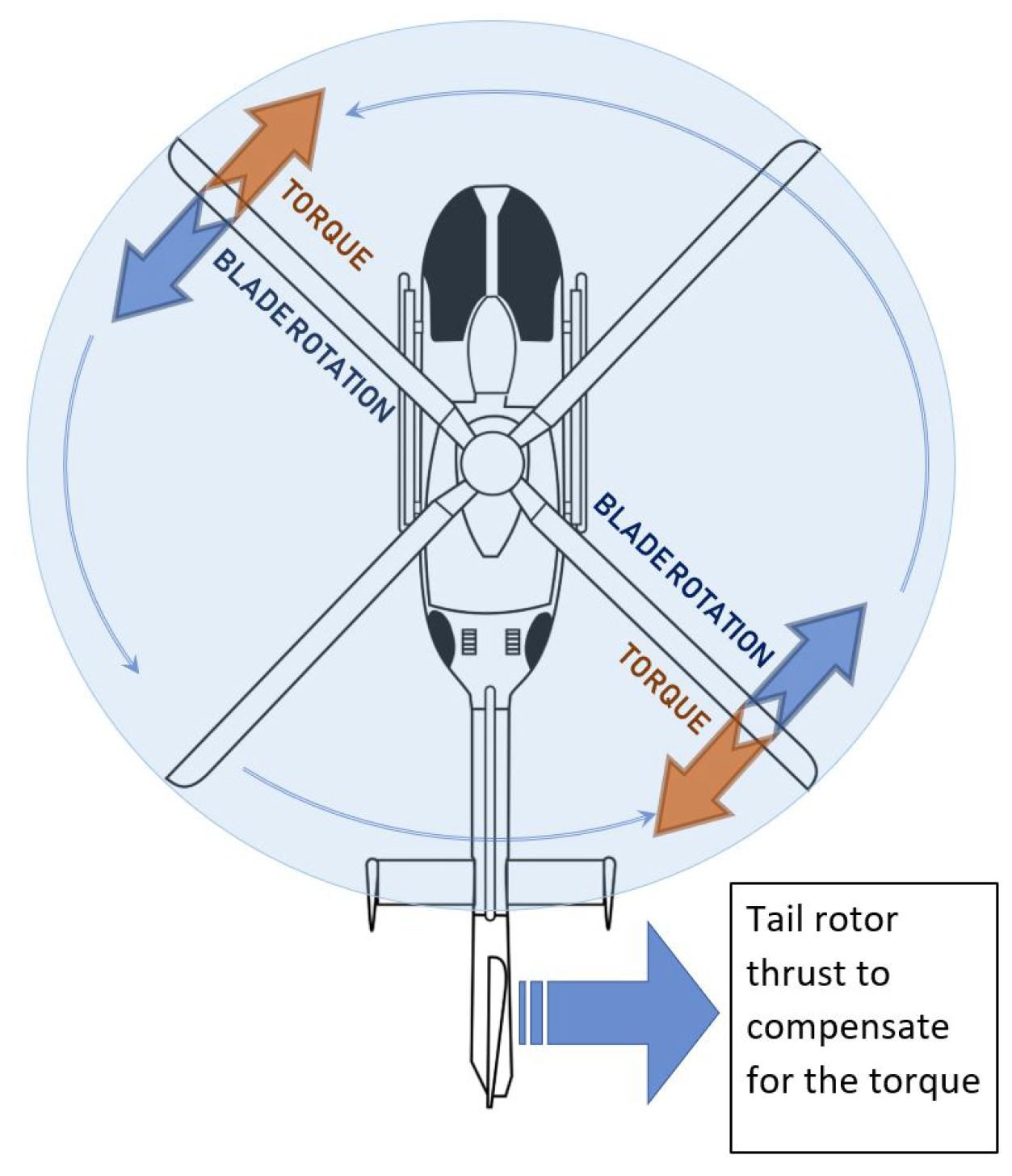
Conventional helicopters are built with two propellers that can be arranged as two coplanar rotors both providing upward thrust, but spinning in opposite directions in order to balance the torques exerted upon the body of the helicopter, or as one main rotor providing thrust and a smaller side rotor oriented laterally and counteracting the torque produced by the main rotor, as shown in the Figure 1. Helicopters with no tail rotors (‘notar’) use a jet of compressed air to compensate for the unwanted yawing of the fuselage.

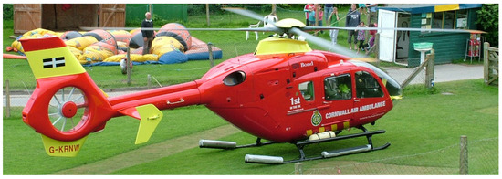
Figure 1. Eurocopter EC 135, with a fantail assembly tail rotor (reproduced from https://en.wikipedia.org/wiki/Tail_rotor accessed on 21 April 2021).

Controls on a helicopter are numerous. Considering a rigid rotor system, the attitude and the position of a helicopter are mainly controlled through two systems, called the collective control system and cyclic control system. The power exerted by the rotors is usually constant, in fact, the blades are designed to operate at a specific rotational speed. However, it is possible to slightly vary the engine power using the throttle control, whereas the direction the aircraft nose points, the yaw angle, could be changed using the pedals control. A summary of helicopter controls is given in the following.

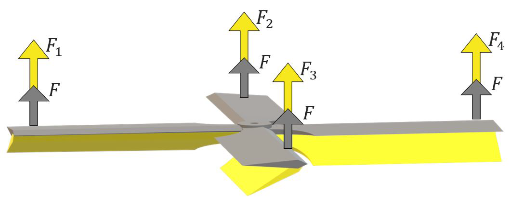
Collective control: The collective control is used to increase or decrease the total thrust generated by the rotors. This technique is adopted in the main rotor and in the tail rotor. To grow (to reduce) the thrust it is necessary to increase (to decrease) the angle of attack ${\alpha }_{\mathrm{c}}$ of all blades. This angle is in each instant the same for all the blades. An example of the usage of the collective control is illustrated in Figure 2.

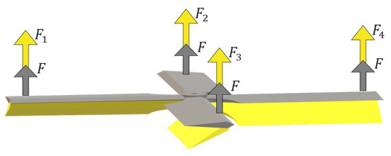
Figure 2. Collective control changes the angle of attack of all blades at the same time. The main rotor is in the grey position, horizontal to the ground, if not actuated. A maneuver of the collective control brings the blades to rotate independently to the yellow configuration. The force generated by each propeller is represented by F in the standard configuration and by $F_1=F_2=F_3=F_4$ in the collective controlled case.

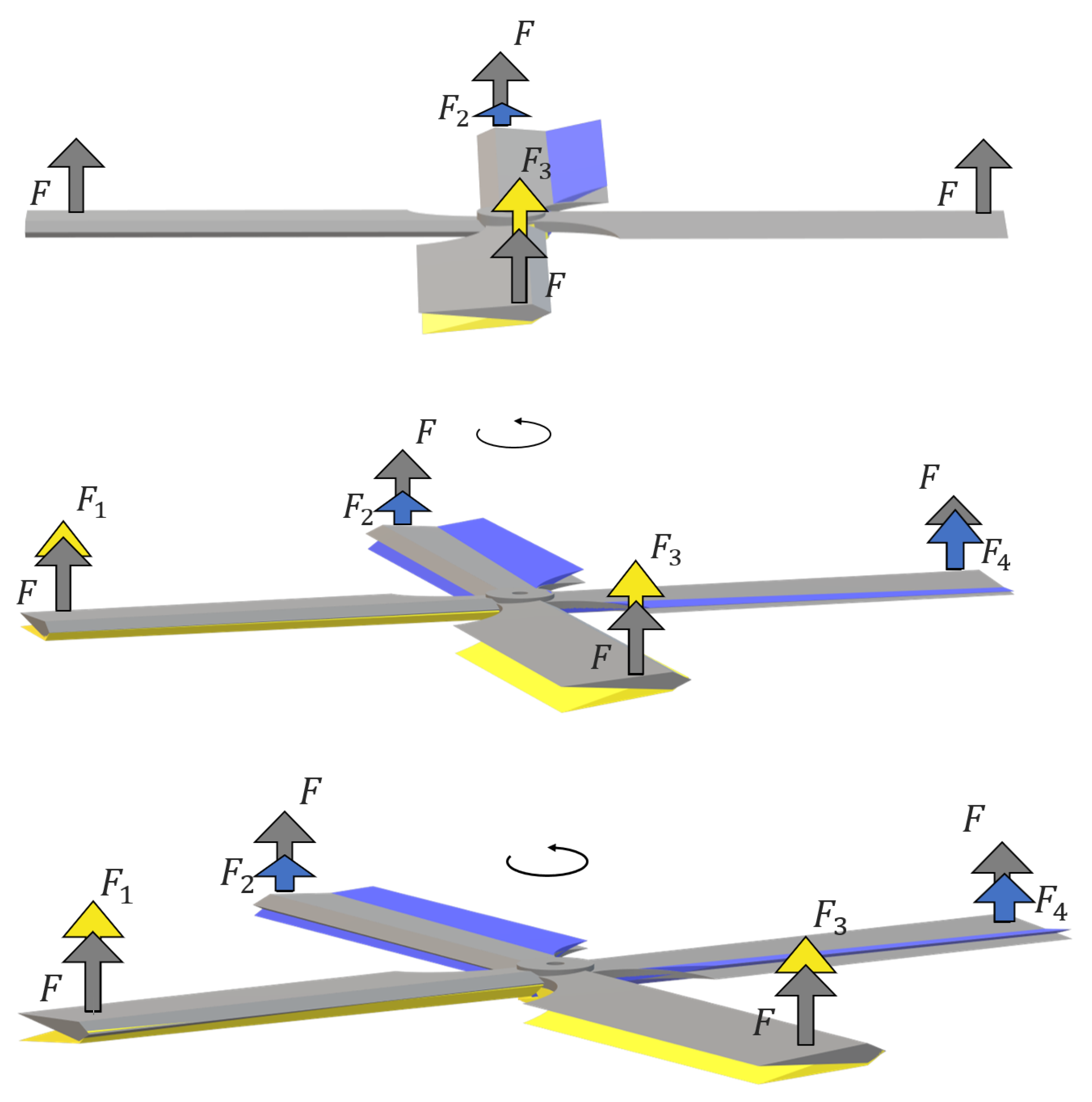
Cyclic control: The cyclic control is distinctive of the main rotor. To tilt the body of a helicopter forward and backwards (pitch) or sideways (roll), a pilot must alter the angle of attack of the main rotor blades cyclically during rotation, as illustrated in Figure 3. In particular, controlling the angle of attack of the blades in such a way that the forward half of the rotor disk exerts more (less) thrust than the backward half makes the helicopter pitch upward (downward). Generally, to vary the attitude of a helicopter it is necessary to modify the angle of the thrust exerted by the main rotor, which is generated by the rotation of the blades, hence it is necessary to create different amounts of thrust at different points in the cycle. Where a greater (smaller) amount of thrust is necessary the blade increases (decrease) its angle. Two angles, namely ${\alpha }_{\mathrm{p}}$ and ${\alpha }_{\mathrm{r}}$, are used to indicate the direction of the thrust vector generated by the main rotor.

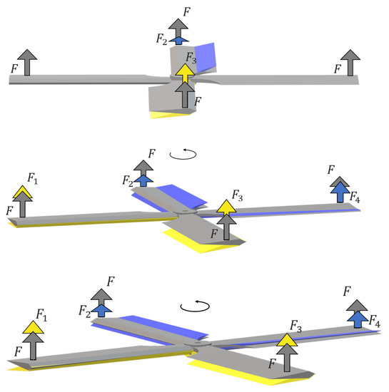
Figure 3. Series of frames representing the rotation of the main rotor actuated by the Cyclic control. The artwork shows the forces exerted by each blade during a rotation. The grey arrow denotes the force F produced when the blade is horizontal, whereas the yellow (blue) arrows denote the forces produced when the angle taken by the blade is such that the thrust is stronger (weaker) than F.

Pedals control: Because of momentum conservation, the rotation of the main rotor causes a rotation of the body of the helicopter in the opposite direction: as the engine turns the main rotor system in a counterclockwise direction, the helicopter fuselage turns clockwise. The amount of torque is directly related to the amount of engine power being used to turn the main rotor system. The unwanted yawing of the fuselage may be balanced by controlling the thrust of the tail rotor, as illustrated in Figure 4. The anti-torque pedals change the tail rotor collective angle of attack ${\alpha }_{\mathrm{c}}^{\mathrm{T}}$. The yaw angle variation depends upon variations of the tail rotor thrust or variations on the main rotor thrust. The pedals control is used for heading changes while hovering, but also to maintain the actual helicopter nose direction.

Figure 4. Anti-torque effect of the tail rotor.

Actuators: The mentioned pilot control systems are actuated through a series of devices that are briefly described in the following:

• The cyclic control and the collective control of the main rotor work through a complex mechanical system called ‘swash-plate’, whose functioning is illustrated, e.g., at page 272 of the manual [1]. The swash-plate is composed of two parts, one that is tight with the rotor mast and one that can rotate with the main rotor. Each blade is strictly connected with the swash-plate revolving part using a rod. This causes a variation of the angle of attack of the blade when the swash-plate changes position. The swash-plate manages the cyclic and collective angles and sets up constraints in their ranges. The collective control causes a movement upward or downward of the swash-plate on the rotor mast, therefore all the blades increase or decrease their angle of attack simultaneously. The cyclic control changes the attitude of the swash-plate. This causes a changing of the angle of attack that is different in every part of the rotation cycle.
• The tail rotor actuator is called a “pitch change spider” and, similarly to the swash-plate, it is used to vary all the angles of attack of the blades simultaneously. A figure at page 272 of the manual [1] illustrates the functioning of the pitch change spider. Helicopters, usually, possess a stabilizer that reduces the noise of the wind, providing an easier use of the yaw pedals. The pitch change spider also sets up the constraints for the range of variation of its angle of attack ${\alpha }_{\mathrm{c}}^{\mathrm{T}}$.

Throttle: The throttle controls the power of the engine which is connected to both rotors by the transmission. The throttle setting must maintain enough engine power to keep the rotor speed within the limits where the rotor produces enough lift for flight. The throttle changes the blades’ angular velocity in a range of few values percentage. Helicopters possess only a gear to drive both the main rotor and tail rotor, hence increasing the speed of the main rotor causes an increase in the tail rotor speed. More throttle means more speed and hence a larger value of thrust. The angular velocity of the rotors is usually reported in percentage for a more intuitive perception, the value of $100\%$ is the typical one under standard conditions.

A helicopter is an extraordinarily complicated machine, whose functioning is based on a number of mechanical devices whose actions interact intricately to one another. Such complex design make its modeling and control by a pilot a fascinating challenge. The main challenge encountered during the present research work was to design a mathematical model that, on one hand, is able to capture the essential features of a helicopter, hence being sufficiently accurate to predict its behavior and, on the other hand, to be simple enough for the result to be mathematically tractable.

In the present paper, we derive, through the Euler–Poincaré formalism, the mathematical model of a simplified helicopter. The model concerns a helicopter with a principal rotor and a tail rotor. More accurate (and mathematically complicated) aircraft models are available in the specialized literature [2,3,4]. The structure of the present paper may be outlined as follows:

• Section 2 presents a summary of definitions and properties regarding Lie groups, such as the tools used in this research to formalize the mathematical model of a helicopter, i.e., tangent bundle, Lie algebra and exponential map. Moreover, this section introduces a system of differential equations that are used to describe the motion of a helicopter.
• Section 3 introduces the structure of the helicopter, a reference system and the structure of forces used to complete the mathematical model, as the thrust of the rotors. In addition, this section outlines a derivation of the equations of motion starting from a Lagrangian function.
• Section 4 presents a numerical scheme to simulate on a computing platform the system of equations determined in Section 3 using a forward Euler (fEul) method tailored to the Lie group of rotations.
• Section 5 introduces a helicopter type and shows the values of the parameters required to perform simulation analysis. These values are presented in tables and figures and have been gathered (and calculated) from data-sheets.
• Section 6 illustrates eight simulation results. Each simulation is particularly focused on a specific response, i.e., pitch response and roll response.
• Section 7 concludes this paper with a recapitulation of the obtained results and an overview of the key points of the performed analysis.

We would like to mention that the scientific literature about system modeling (including mechanical system modeling) is rich in inventions. A few alternative techniques to the more traditional equation-based modeling and control are bond graph modeling utilized, e.g., in [5] to design a Kalman filter observer for an industrial back-support exoskeleton; closed loop identification and frequency domain analysis, utilized in [6] to determine a dynamic model of a quadrotor prototype; deep neural networks, used in [7] to predict the remaining useful life (RUL) of aircraft gas turbine engines. The present authors are not familiar enough with the mentioned techniques to judge their advantages or disadvantages in relation to the proposed modeling method, which arises as a more elaborated version of the familiar Euler–Lagrange formalism (except for the neural-network modeling approach that provides an approximated, data-derived model in contrast to exact models).

2. The Lagrange–d’Alembert–Pontryagin Principle and the Forced Euler–Poincaré Equation

In this paper, we consider non-conservative non-linear dynamical systems whose state space $\mathbb{G}$ possesses the mathematical structure of a Lie group.

2.1. Definition and Properties

Let us recapitulate the following definitions and properties [8,9] (see also [10,11] for a non-strictly mathematical viewpoint):

Matrix Lie group: A smooth matrix manifold $\mathbb{G}$ that is also an algebraic group is termed a matrix Lie group. A matrix group is a matrix set endowed with an associative binary operation, termed group multiplication which, for any two elements $g,h\in \mathbb{G}$, is denoted by $gh$, endowed with the property of closure, an identity element with respect to the multiplication, denoted by e, such that $eg=ge=g$ for any $g\in \mathbb{G}$, and an inversion operation, denoted by $g^{-1}$, with respect to multiplication, such that $g^{-1}g=g{g}^{-1}=e$ for any $g\in \mathbb{G}$. A left translation $L:\mathbb{G}\times \mathbb{G}\to \mathbb{G}$ is defined as $L_g(h):=g^{-1}h$. An instance of matrix Lie group is $\mathrm{SO}(3):=\{R\in {\mathbb{R}}^{3\times 3}\mid R^{\top }R=R{R}^{\top }=I_3,det(R)=+1\}$, where the symbol ${}^{\top }$ denotes matrix transposition and the quantity $I_3$ represents a $3\times 3$ identity matrix.

Tangent bundle and its metrization: Given a point $g\in \mathbb{G}$, the tangent space to $\mathbb{G}$ at g will be denoted as $T_g\mathbb{G}$. The tangent bundle associated with a manifold-group $\mathbb{G}$ is denoted by $T\mathbb{G}$ and plays the role of phase-space for a dynamical system whose state-space is $\mathbb{G}$. The inner product of two tangent vectors $\xi ,\eta \in T_g\mathbb{G}$ is denoted by ${⟨\xi ,\eta ⟩}_g$. A smooth function $F:\mathbb{G}\to \mathbb{G}$ induces a linear map $\mathrm{d}{F}_g:T_g\mathbb{G}\to T_{F(g)}\mathbb{G}$ termed pushforward map. For a matrix Lie group, the pushforward map $\mathrm{d}{(L_g)}_h:T_h\mathbb{G}\to T_{L_g(h)}\mathbb{G}$ associated with a left translation is $\mathrm{d}{(L_g)}_h(\eta ):=g^{-1}\eta$, with $\eta \in T_h\mathbb{G}$.

Lie algebra: The tangent space $\mathfrak{g}:=T_e\mathbb{G}$ to a Lie group at the identity is termed Lie algebra. The Lie algebra is endowed with Lie brackets, denoted as $[·,·]:\mathfrak{g}\times \mathfrak{g}\to \mathfrak{g}$, and an adjoint endomorphism ${\mathrm{ad}}_{\xi }\eta :=[\xi ,\eta ]$. The Lie algebra associated with the group $\mathrm{SO}(3)$ is $\mathfrak{so}(3):=\{\xi \in {\mathbb{R}}^{3\times 3}\mid \xi +{\xi }^{\top }=0\}$. On a matrix Lie algebra, the Lie brackets coincide with matrix commutator, namely $[\xi ,\eta ]:=\xi \eta -\eta \xi$. The matrix commutator in $\mathfrak{so}(3)$ is an anti-symmetric bilinear form, namely $[\xi ,\eta ]+[\eta ,\xi ]=0$. A pushforward map $\mathrm{d}{(L_g)}_g:T_g\mathbb{G}\to \mathfrak{g}$ is denoted as $\mathrm{d}{L}_g$ for brevity. Given a smooth function $\ell :\mathfrak{g}\to \mathbb{R}$, for a matrix Lie group one may define the fiber derivative of ℓ, $\frac{\partial \ell }{\partial \xi }\in \mathfrak{g}$, at $\xi \in \mathfrak{g}$ as the unique algebra element such that ${⟨\frac{\partial \ell }{\partial \xi },\eta ⟩}_e=\mathrm{tr}({({\mathbf{J}}_{\xi }\ell )}^{\top }\eta )$ for any $\eta \in \mathfrak{g}$, where ${\mathbf{J}}_{\xi }\ell$ denotes the Jacobian matrix of the function ℓ with respect to the matrix $\xi$. (Notice that ${\mathbf{J}}_{\xi }\ell$ is a formal Jacobian, namely a matrix of partial derivatives with respect to each entry of the matrix $\xi$ without any regard of the internal structure of the matrix $\xi$ itself.)

Exponential map: Given a point $g\in \mathbb{G}$ and a tangent vector $v\in T_g\mathbb{G}$, the exponential maps g to a point ${exp}_g(v)$, namely, it flows the point g along a geodesic line departing from g with initial direction v. On a matrix Lie group endowed with the Euclidean metric, it holds that ${exp}_g(v)=g\mathrm{Exp}(g^{-1}v)$, where ‘$\mathrm{Exp}$’ denotes a matrix exponential.

2.2. The Euler–Poincaré Equations

The Lagrange–d’Alembert–Pontryagin (LDAP) principle is one of the fundamental concepts in mathematical physics to describe the time-evolution of the state of a physical system and to handle non-conservative external forces. The state-variables of the system are subjected to holonomic constraints, which are embodied in the structure of the state Lie group $\mathbb{G}$. These external forces often arise as control actions designed with the aim of driving the physical system into a predefined state [12]. Let $\mathsf{\Lambda }:T\mathbb{G}\to \mathbb{R}$ denote a Lagrangian function and $F:T\mathbb{G}\to T\mathbb{G}$ a generalized force field. (A generalized force field is generally taken as a smooth map from $T\mathbb{G}$ to its dual $T^{\star }\mathbb{G}$ or, for left-invariant force fields, from an algebra $\mathfrak{g}$ to its dual ${\mathfrak{g}}^{\star }$. We adopt a non-standard definition because it eases the notation and is more easily translated into implementation). The LDAP principle affirms that a dynamical system follows a trajectory $g:[a,b]\to \mathbb{G}$ such that:

$$\delta {\int }_a^b\mathsf{\Lambda }(g(t),\dot{g}(t))\mathrm{d}t+{\int }_a^b{⟨F(g(t),\dot{g}(t)),\delta g(t)⟩}_{g(t)}\mathrm{d}t=0,$$

(1)

The leftmost integral is called action and the symbol $\delta$ denotes variation, namely the change of the action value from a trajectory g to a trajectory that is infinitely close to g, whose point-by-point change is denoted as $\delta g$. The variation vanishes at endpoints and is elsewhere arbitrary. In the above expression, an over-dot (as in $\dot{g}$) denotes derivation with respect to the parameter t. The vanishing of the first term alone is called principle of stationary action. The rightmost integral represents the total work achieved by the force field F due to the variation.

A variational formulation is based on a smooth family of curves $g:U\subset {\mathbb{R}}^2\to \mathbb{G}$, where each element is denoted as $g(t,\epsilon )$. The index $\epsilon$ selects a curve in the family, and the index t individuates a point over this curve. All the curves in the family depart from the same initial point and arrive at the same endpoint, namely, $g(a,\epsilon )$ and $g(b,\epsilon )$ are constant with respect to $\epsilon$. The variations in (1) are defined as

$$\begin{array}{c}\hfill \delta {\int }_a^b\mathsf{\Lambda }(g,\dot{g})\mathrm{d}t:={\left.{\int }_a^b\frac{\partial }{\partial \epsilon }\mathsf{\Lambda }(g(t,\epsilon ),\dot{g}(t,\epsilon ))\mathrm{d}t\right|}_{\epsilon =0},\delta g(t):={\left.\frac{\partial g(t,\epsilon )}{\partial \epsilon }\right|}_{\epsilon =0}.\end{array}$$

(2)

The following result, enunciated directly for matrix Lie groups, is of prime importance, as it relates a variation of velocity to velocity of variation.

Lemma 1

([13]). Given a smooth function $g:U\subset {\mathbb{R}}^2\to \mathbb{G}$ on a matrix Lie group, define:

$$\begin{array}{c}\hfill \xi (t,\epsilon ):=g^{-1}(t,\epsilon )\frac{\partial g(t,\epsilon )}{\partial t},\eta (t,\epsilon ):=g^{-1}(t,\epsilon )\frac{\partial g(t,\epsilon )}{\partial \epsilon }.\end{array}$$

(3)

A variation of a trajectory induces a variation of its velocity field given by

$$\frac{\partial \xi }{\partial \epsilon }=\dot{\eta }+{\mathrm{ad}}_{\xi }\eta .$$

(4)

Assuming that the Lagrangian as well as the generalized force field F are left invariant, we may write $\mathsf{\Lambda }(g,\dot{g})=\ell (g^{-1}\dot{g})$ and $g^{-1}F(g,\dot{g})=f(g^{-1}\dot{g})$, where $\ell :\mathfrak{g}\to \mathbb{R}$ and $f:\mathfrak{g}\to \mathfrak{g}$ denote a reduced Lagrangian and a reduced force field, respectively. In addition, if the inner product is left-invariant, it holds that

$${⟨F(g,\dot{g}),\delta g⟩}_g={⟨f(g^{-1}\dot{g}),g^{-1}\delta g⟩}_e.$$

(5)

Therefore, the LDAP principle (1) reduces to

$$\delta {\int }_a^b\ell (g^{-1}\dot{g})\mathrm{d}t+{\int }_a^b{⟨f(g^{-1}\dot{g}),g^{-1}\delta g⟩}_e\mathrm{d}t=0,$$

(6)

where it is legitimate to replace $g^{-1}\dot{g}$ with $\xi$ and $g^{-1}\delta g$ with $\eta$ and then set $\epsilon$ to 0.

By means of the Lemma 1, the variational formulation of the reduced LDAP principle may be recast in a differential form.

Theorem 1

([13]). Let $\xi :=g^{-1}\dot{g}$ and $\eta :=g^{-1}\delta g$. The solution of the integral Lagrange–d’Alembert equation (6) under perturbations of the form $\frac{\partial \xi }{\partial \epsilon }=\dot{\eta }+{\mathrm{ad}}_{\xi }\eta$, which vanishes at endpoints, satisfies the Euler–Poincaré equation

$$\frac{\mathrm{d}}{\mathrm{d}t}\frac{\partial \ell }{\partial \xi }={\mathrm{ad}}_{\xi }^{\star }\left(\frac{\partial \ell }{\partial \xi }\right)+f,$$

(7)

where ${\mathrm{ad}}^{\star }$ denotes the adjoint (The adjoint ${\omega }^{\star }$ of an operator $\omega :\mathfrak{g}\to \mathfrak{g}$ with respect to an inner product $⟨·,·⟩$ satisfies $⟨\omega (\xi ),\eta ⟩=⟨\xi ,{\omega }^{\star }(\eta )⟩$.) of the operator $\mathrm{ad}$ with respect to the inner product of $\mathfrak{g}$.

The complete system of differential equations then read

$$\left\{\begin{array}{ccc}\dot{g}\hfill & =& g\xi ,\hfill \\ \frac{\mathrm{d}}{\mathrm{d}t}\frac{\partial \ell }{\partial \xi }\hfill & =& {\mathrm{ad}}_{\xi }^{\star }\left(\frac{\partial \ell }{\partial \xi }\right)+f.\hfill \end{array}\right.$$

(8)

The above equations may be used to describe the rotational component of motion of a flying object such as a helicopter or a drone. The forcing term takes into account several external driving phenomena, such as:

Energy dissipation: Energy dissipation is due, e.g., to friction with air particles. For instance, a linear dissipation term represents aerodynamic drag.

Control actions: Other than dissipation (which is often neglected in simplistic models), the forcing term depends on the problem under investigation. It might serve to incorporate into the equations control terms aimed, for instance, at stabilizing the motion or to drive a dynamical system [14].

2.3. Particular Case: Euclidean Space

In order to clarify the physical meaning of the Euler–Poincaré equations, let us recall the classical version of these equations for the space ${\mathbb{R}}^n$, which is also instrumental in describing the translational component of motion of a flying device. The principle (1) on ${\mathbb{R}}^n$, endowed with the Euclidean inner product, reads:

$$\delta {\int }_a^b\mathsf{\Lambda }(p(t),\dot{p}(t))\mathrm{d}t+{\int }_a^{b}f{(p(t),\dot{p}(t))}^{\top }\delta p(t)\mathrm{d}t=0,$$

(9)

where $\mathsf{\Lambda }:{\mathbb{R}}^n\times {\mathbb{R}}^n\to \mathbb{R}$ denotes a Lagrangian function, $p=p(t)$ a trajectory in ${\mathbb{R}}^n$ and $f:{\mathbb{R}}^n\times {\mathbb{R}}^n\to {\mathbb{R}}^n$ a non-conservative force field. Upon computing the variation, we obtain

$${\int }_a^b\left({\left(\frac{\partial \mathsf{\Lambda }}{\partial p}\right)}^{\top }\delta p+{\left(\frac{\partial \mathsf{\Lambda }}{\partial \dot{p}}\right)}^{\top }\delta \dot{p}+f^{\top }\delta p\right)\mathrm{d}t=0.$$

(10)

Integrating by parts the second term and recalling that the variations vanish at the endpoints, we obtain

$${\int }_a^b{\left(\frac{\partial \mathsf{\Lambda }}{\partial p}-\frac{\mathrm{d}}{\mathrm{d}t}\frac{\partial \mathsf{\Lambda }}{\partial \dot{p}}+f\right)}^{\top }\delta p\mathrm{d}t=0.$$

(11)

Since the variation $\delta p$ is arbitrary, the dynamics of the variable p is governed by the Euler–Lagrange equation

$$\frac{\mathrm{d}}{\mathrm{d}t}\frac{\partial \mathsf{\Lambda }}{\partial \dot{p}}=\frac{\partial \mathsf{\Lambda }}{\partial p}+f$$

(12)

where the quantity $q:=\frac{\partial \mathsf{\Lambda }}{\partial \dot{p}}$ is usually termed linear momentum.

3. Mathematical Model of a Helicopter

This section introduces a helicopter model based on the Lie group $\mathbb{G}:=\mathrm{SO}(3)$ of the 3-dimensional rotations R.

Since, in the state space $\mathbb{G}:=\mathrm{SO}(3)$, it holds that ${(\mathrm{d}{L}_R)}^{-1}(\xi )=R\xi$ and ${\mathrm{ad}}_{\xi }^{\star }\eta =-{\mathrm{ad}}_{\xi }\eta$ [13], the Euler–Poincaré equations read

$$\left\{\begin{array}{c}\dot{R}=R\xi ,\hfill \\ \frac{\mathrm{d}}{\mathrm{d}t}\frac{\partial \ell }{\partial \xi }=-{\mathrm{ad}}_{\xi }\left(\frac{\partial \ell }{\partial \xi }\right)+\tau ,\hfill \end{array}\right.$$

(13)

where $\tau$ denotes the resultant of all external mechanical torques. In this context, the state variable $R\in \mathrm{SO}(3)$ denotes the attitude of a rigid body (i.e., its orientation with respect to a earth-fixed reference frame) and the state-variable $\xi \in \mathfrak{so}(3)$ denotes its instantaneous angular velocity. Moreover, the quantity $\mu :=\frac{\partial \ell }{\partial \xi }$ represents an angular momentum and the second Euler–Poincaré equation reads $\dot{\mu }=[\mu ,\xi ]+\tau$, which is a generalization of the well-known angular momentum theorem, where the term $[\mu ,\xi ]$ represents the inertial torque due to the internal mass unbalance of a body.

It is convenient to define the operator $〚·〛:{\mathbb{R}}^3\to \mathfrak{g}$ as:

$$x:=\left[\begin{array}{c}{x}_1\\ x_2\\ x_3\end{array}\right]\mapsto 〚x〛:=\left[\begin{array}{ccc}0& -x_3& x_2\\ x_3& 0& -x_1\\ -x_2& x_1& 0\end{array}\right].$$

(14)

Since any skew-symmetric matrix in $\mathfrak{so}(3)$ may be written as in (14), it is convenient to define a basis of $\mathfrak{so}(3)=\mathrm{span}({\xi }_x,{\xi }_y,{\xi }_z)$ as follows:

$${\xi }_x:=\left[\begin{array}{ccc}0& 0& 0\\ 0& 0& -1\\ 0& 1& 0\end{array}\right],{\xi }_y:=\left[\begin{array}{ccc}0& 0& 1\\ 0& 0& 0\\ -1& 0& 0\end{array}\right],{\xi }_z:=\left[\begin{array}{ccc}0& -1& 0\\ 1& 0& 0\\ 0& 0& 0\end{array}\right].$$

(15)

In order to shorten some relations, it is also convenient to introduce the matrix anti-commutator $\{A,B\}:=AB+BA$. Moreover, some relations take advantage of the skew-symmetric projection $\left\{\{·\}\right\}:{\mathbb{R}}^{3\times 3}\to \mathfrak{so}(3)$, defined as $\left\{\left\{A\right\}\right\}:=\frac{1}{2}(A-A^{\top })$. It also pays to define the ‘diag’ operator as $\mathrm{diag}(a,b,c):=\left[\begin{array}{ccc}a& 0& 0\\ 0& b& 0\\ 0& 0& c\end{array}\right]$.

In the present setting, we equip the algebra $\mathfrak{so}(3)$ with the canonical metric ${⟨\xi ,\eta ⟩}_e:=\mathrm{tr}({\xi }^{\top }\eta )$. With this choice, the fiber derivative of a scalar function $\ell :\mathfrak{so}(3)\to \mathbb{R}$ takes a special form.

Lemma 2

([15]). The fiber derivative of a scalar function $\ell :\mathfrak{so}(3)\to \mathbb{R}$ under the canonical metric takes the form

$$\frac{\partial \ell }{\partial \xi }=\frac{1}{2}({\mathbf{J}}_{\xi }\ell -{\mathbf{J}}_{\xi }^{\top }\ell )\in \mathfrak{so}(3).$$

(16)

It is immediate to verify that the fiber derivative corresponds to the orthogonal projection of the Jacobian into the algebra $\mathfrak{g}$, namely $\frac{\partial \ell }{\partial \xi }=\left\{\{{\mathbf{J}}_{\xi }\ell \}\right\}$. Moreover, it is convenient to recall a property of the matrix ‘trace’ operator, namely the cyclic permutation property $\mathrm{tr}(ABC)=\mathrm{tr}(BCA)=\mathrm{tr}(CAB)$ for any square conformable matrices $A,B,C$.

Modeling a complex object to obtain the differential equations that describe its rotational and translational dynamics consists essentially in:

• Defining a Lagrangian function ℓ on the basis of the kinetic and potential energy of its components, which accounts for the geometrical and mechanical features of each component;
• Computing the total mechanical torque $\tau$ exerted by the moving parts on the body of the complex object.

These descriptors, for a helicopter, are evaluated in the next subsections.

3.1. Model of a Helicopter with a Single Principal Rotor and a Tail Rotor

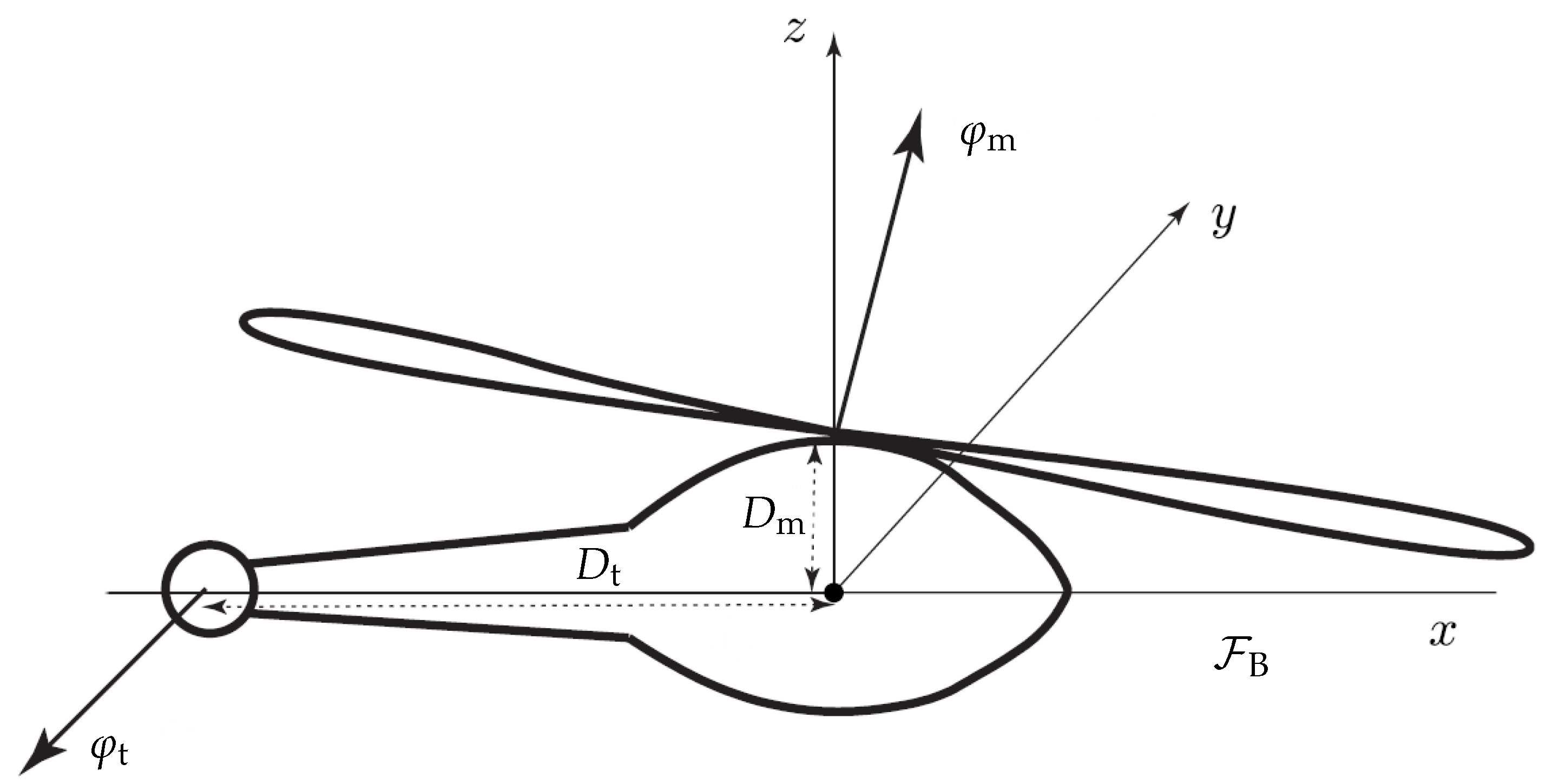
In order to formalize the behavior of a helicopter into a mathematical model, let us fix an inertial (earth) reference frame ${\mathcal{F}}_{\mathrm{E}}$. Further, it is necessary to establish a body-fixed reference frame ${\mathcal{F}}_{\mathrm{B}}$, as shown in Figure 5: the origin of the reference frame ${\mathcal{F}}_{\mathrm{B}}$ is located at the center of gravity of the helicopter and the three axes coincide with its principal inertia axes. The thrust ${\phi }_{\mathrm{m}}$ exerted by the principal rotor appears at the tip of the helicopter’s body, which is located along the z-axis at a distance $D_{\mathrm{m}}$ from the center of gravity, whereas the thrust ${\phi }_{\mathrm{t}}$ exerted by the tail rotor appears at the tail of the helicopter’s body, which is located along the $-x$ axis at a distance $D_{\mathrm{t}}$ from the center of gravity.

Figure 5. Schematic of a helicopter with a principal rotor and a tail rotor (adapted from [12]). (The principal rotor to center of mass distance $D_{\mathrm{m}}$ and the tail rotor to center of mass distance $D_{\mathrm{t}}$ are expressed in meters (m).)

Furthermore, the term $\frac{1}{2}{u}_{\mathrm{m}}$ represents the intensity of the thrust exerted by the main rotor, while $\frac{1}{2}{u}_{\mathrm{t}}$ denotes the thrust exerted by the tail rotor, both expressed in Newtons (N). Considering the total thrust $\phi :={\phi }_{\mathrm{t}}+{\phi }_{\mathrm{m}}$ as a vector, a collective control management of the main rotor results in a change of the thrust intensity exerted, namely a change in $u_{\mathrm{m}}$, whereas a cyclic control management changes the direction of the lift exerted, therefore the pitch angle ${\alpha }_{\mathrm{p}}$ (in radians (rad)) and the sideways roll angle ${\alpha }_{\mathrm{r}}$ (in radians). The expressions of the thrusts (from [12]) and of their moment arms in the helicopter’s body-fixed frame ${\mathcal{F}}_{\mathrm{B}}$ are given by

$${\phi }_{\mathrm{m}}:=\frac{1}{2}{u}_{\mathrm{m}}\left[\begin{array}{c}sin{\alpha }_{\mathrm{p}}cos{\alpha }_{\mathrm{r}}\\ -sin{\alpha }_{\mathrm{r}}\\ cos{\alpha }_{\mathrm{p}}cos{\alpha }_{\mathrm{r}}\end{array}\right],b_{\mathrm{m}}:=\left[\begin{array}{c}0\\ 0\\ D_{\mathrm{m}}\end{array}\right],$$

(17)

$${\phi }_{\mathrm{t}}:=\frac{1}{2}{u}_{\mathrm{t}}\left[\begin{array}{c}0\\ -1\\ 0\end{array}\right],b_{\mathrm{t}}:=\left[\begin{array}{c}-D_{\mathrm{t}}\\ 0\\ 0\end{array}\right].$$

(18)

The vector $\frac{2{\phi }_{\mathrm{m}}}{u_{\mathrm{m}}}$ may be regarded as the unit normal to the rotor disk [2]. A further forcing term to account for the resistance of the air during forward vertical motion is described in Section 3.4. Concerning the thrust generated by the principal rotor, we may notice what follows:

• Whenever ${\alpha }_{\mathrm{r}}={\alpha }_{\mathrm{p}}=0$, the thrust takes the expression $\frac{1}{2}{u}_{\mathrm{m}}\left[\begin{array}{c}0\\ 0\\ 1\end{array}\right]$, namely, only the z-component is non-null and the thrust is vertical;
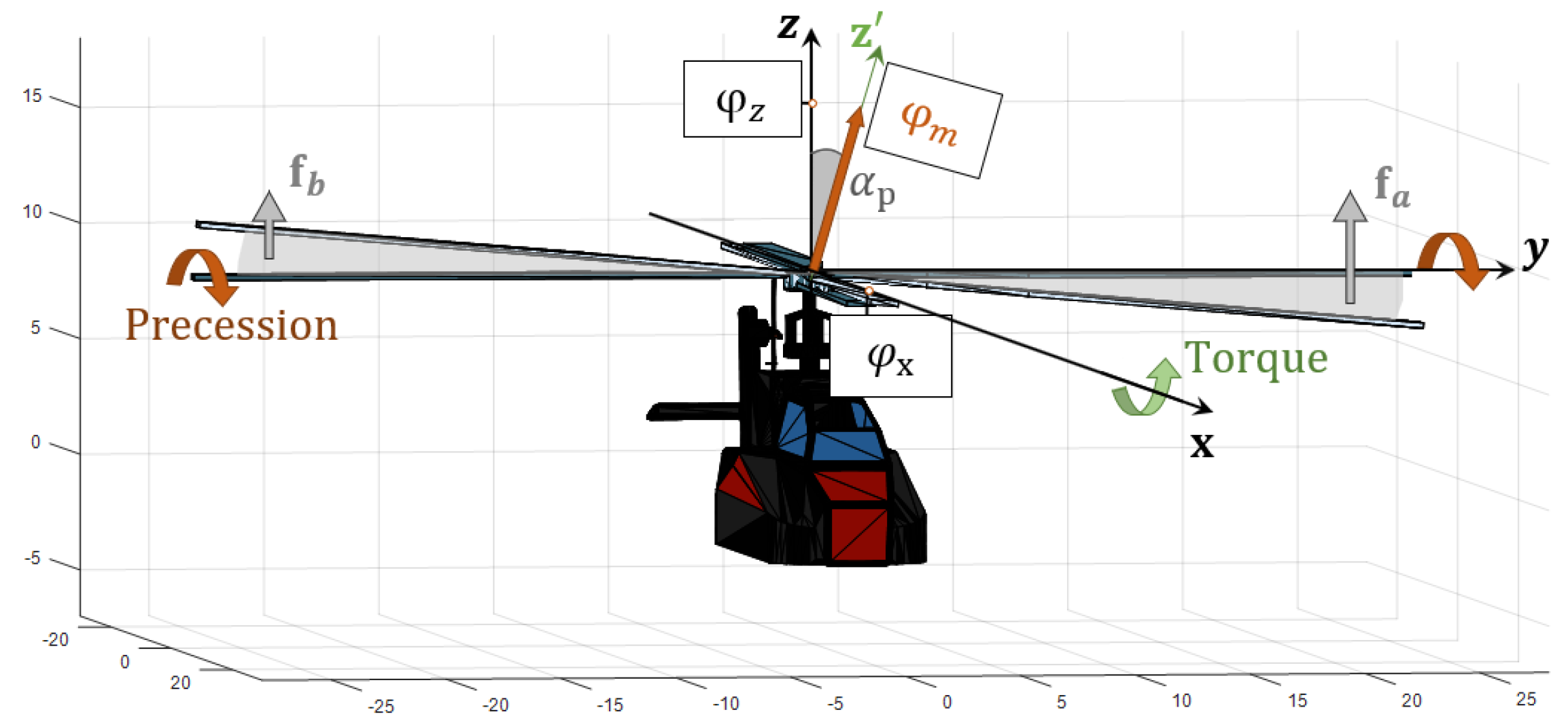
• Whenever ${\alpha }_p=0$ and ${\alpha }_{\mathrm{r}}\ne 0$, the thrust takes the expression $\frac{1}{2}{u}_{\mathrm{m}}\left[\begin{array}{c}0\\ -sin{\alpha }_{\mathrm{r}}\\ cos{\alpha }_{\mathrm{r}}\end{array}\right]$, namely, the x-component is null and the thrust belongs to the y–z plane, as shown in Figure 6, hence it may only produce a rotation along the x-axis, which corresponds to pure rolling. (Remark: The right-hand law defines the positive angle variation.)
  

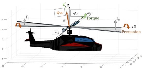  Figure 6. Illustration of a positive variation of the angle of attack along the x-axis, where ${\phi }_y=-\frac{1}{2}{u}_{\mathrm{m}}sin{\alpha }_{\mathrm{r}}$ and ${\phi }_z=\frac{1}{2}{u}_{\mathrm{m}}cos{\alpha }_{\mathrm{r}}$ are the projections of the thrust vector ${\phi }_{\mathrm{m}}$ along the y- and z-axis, respectively. The maneuver to control rolling assigns to the blades an angle such that a greater amount of force is produced in the positive x-axis, namely $f_a$, with respect to the force in the negative x-axis, namely $f_b$. Those two vector forces produce a torque and a precession rotation due to the gyroscopic effect.
• whenever ${\alpha }_r=0$ and ${\alpha }_p\ne 0$, the thrust takes the expression $\frac{1}{2}{u}_{\mathrm{m}}\left[\begin{array}{c}sin{\alpha }_{\mathrm{p}}\\ 0\\ cos{\alpha }_{\mathrm{p}}\end{array}\right]$, namely, the y-component is null and the thrust belongs to the x–z plane, as shown in Figure 7, hence it may only produce a rotation along the y-axis, which corresponds to pure pitching.
  

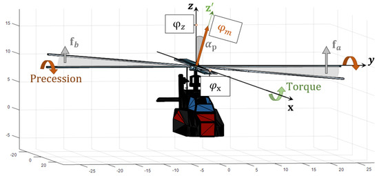  Figure 7. Illustration of a positive variation of the angle of attack along the y-axis, where ${\phi }_x=\frac{1}{2}{u}_{\mathrm{m}}sin{\alpha }_{\mathrm{p}}$ and ${\phi }_z=\frac{1}{2}{u}_{\mathrm{m}}cos{\alpha }_{\mathrm{p}}$ are the projections of the main rotor thrust ${\phi }_{\mathrm{m}}$ to the x- and z-axis, respectively. The maneuver to control the pitching assigns to the blades an angle such that a larger amount of force is produced in the positive y-axis, namely $f_a$, with respect to the force along the negative y-axis, namely $f_b$. Those two vector forces produce a mechanical torque and a precession of the fuselage.

Notice that the inclination of the blades influences the thrust and the torque acting on the fuselage, but does not influence directly the roll and the pitch attitude of the helicopter. Further, notice that the thrust $\frac{1}{2}{u}_{\mathrm{m}}$ does not distribute equally across the three directions of space and, in particular, that a change in the angles of attack of the blades weakens the vertical component of the thrust: when a helicopter tilts, it tends to fall, unless the thrust is compensated by the pilot. It is also worth noticing that the total thrust $\phi$ acting on the fuselage has a y component that depends on the tail rotor thrust. This component causes the translation of the helicopter in the direction of ${\phi }_{\mathrm{t}}$: this is called drift effect (or translation tendency). The mechanical torque exerted by the two rotors on the helicopter’s fuselage, expressed in N·m, is termed active torque and is given by

$$\begin{array}{ccc}\hfill {\tau }_{\mathcal{A}}& :=& \frac{1}{2}\left({\phi }_{\mathrm{m}}{b}_{\mathrm{m}}^{\top }-b_{\mathrm{m}}{\phi }_{\mathrm{m}}^{\top }+{\phi }_{\mathrm{t}}{b}_{\mathrm{t}}^{\top }-b_{\mathrm{t}}{\phi }_{\mathrm{t}}^{\top }\right)\hfill \\ & =& \frac{1}{2}\left[\begin{array}{ccc}0& -D_{\mathrm{t}}{u}_{\mathrm{t}}& D_{\mathrm{m}}{u}_{\mathrm{m}}sin{\alpha }_{\mathrm{p}}cos{\alpha }_{\mathrm{r}}\\ D_{\mathrm{t}}{u}_{\mathrm{t}}& 0& -D_{\mathrm{m}}{u}_{\mathrm{m}}sin{\alpha }_{\mathrm{r}}\\ -D_{\mathrm{m}}{u}_{\mathrm{m}}sin{\alpha }_{\mathrm{p}}cos{\alpha }_{\mathrm{r}}& D_{\mathrm{m}}{u}_{\mathrm{m}}sin{\alpha }_{\mathrm{r}}& 0\end{array}\right].\hfill \end{array}$$

(19)

The mechanical torque due to the drag of the principal rotor, namely the resultant of the torque that tends to make the helicopter spin as a counter-reaction to the spinning of the rotor, expressed in N·m, may be quantify by

$${\tau }_{\mathcal{D}}:=-\frac{1}{2}\gamma u_{\mathrm{m}}{\xi }_z,$$

(20)

where $\gamma >0$ is termed air drag coefficient (whose measurement unit is meters) and represents the efficacy with which the air surrounding the helicopter pushes the rotor as a reaction of its spinning. According to the canonical basis (15), the total mechanical torque $\tau :={\tau }_{\mathcal{A}}+{\tau }_{\mathcal{D}}$ may be decomposed as $\tau ={\tau }_x{\xi }_x+{\tau }_y{\xi }_y+{\tau }_z{\xi }_z$, with

$$\left\{\begin{array}{c}{\tau }_x=\frac{1}{2}{D}_{\mathrm{m}}{u}_{\mathrm{m}}sin{\alpha }_{\mathrm{r}},\hfill \\ {\tau }_y=\frac{1}{2}{D}_{\mathrm{m}}{u}_{\mathrm{m}}sin{\alpha }_{\mathrm{p}}cos{\alpha }_{\mathrm{r}},\hfill \\ {\tau }_z=\frac{1}{2}{D}_{\mathrm{t}}{u}_{\mathrm{t}}-\frac{1}{2}\gamma u_{\mathrm{m}}.\hfill \end{array}\right.$$

(21)

The component ${\tau }_x$ is responsible for the rolling of the helicopter (plane y–z), the component ${\tau }_y$ is responsible for the pitching of the helicopter (plane x–z). The component ${\tau }_z$ is responsible for the control of the yawing of the helicopter (plane x–y): to prevent the spinning of the aircraft, it is necessary to control the thrust $u_{\mathrm{t}}$ of the tail rotor in such a way that $D_{\mathrm{t}}{u}_{\mathrm{t}}-\gamma u_{\mathrm{m}}\approx 0$. During hovering, the vertical component of the total thrust needs to balance the weight force of the helicopter. A further torque component is introduced in Section 3.3 to account for friction-type resistance during fast yawing. According to the specialized literature (see, e.g., [16]), the maximum value of the thrust $u_{\mathrm{m}}$ of the main rotor (in Newtons) may be computed by the expression

$$u_{\mathrm{m}}:=\frac{1}{2}{C}_{\mathrm{u}}\rho A{(l_{\mathcal{R}}{\mathsf{\Omega }}_{\mathrm{m}})}^2,$$

(22)

where $C_{\mathrm{u}}$ is a (dimensionless) thrust coefficient that represents the efficiency of the rotor, $\rho$ represents the density of the air at a given temperature and altitude in kg·m${}^{-3}$, A denotes the area of the rotor disk, in ${\mathrm{m}}^2$, which contributes to generating the thrust, $l_{\mathcal{R}}$ represents the radius of the rotor disk (namely, the length of each blade) in meters and ${\mathsf{\Omega }}_{\mathrm{m}}$ denotes the angular velocity of the rotor in rad·s${}^{-1}$. In fact, the product $l_{\mathcal{R}}{\mathsf{\Omega }}_{\mathrm{m}}$ denotes the tip velocity of a blade. Such thrust may be expressed compactly as a quadratic function of the rotor speed as $u_{\mathrm{m}}={\beta }_{\mathrm{u}}{\mathsf{\Omega }}_{\mathrm{m}}^2$. Further, the mechanical power (in Watts) that the engine transfers to the rotor is given by

$$w:=\frac{1}{2}{C}_{\mathrm{w}}\rho A{(l_{\mathcal{R}}{\mathsf{\Omega }}_{\mathrm{m}})}^2{\mathsf{\Omega }}_{\mathrm{m}},$$

(23)

where $C_{\mathrm{w}}$ denotes a (dimensionless) power coefficient. Such power may be expressed as a cubic function of the rotor speed, namely $w={\beta }_{\mathrm{w}}{\mathsf{\Omega }}_{\mathrm{m}}^3$. The main rotor disk area A changes its value thanks to collective control and consequently to ${\alpha }_{\mathrm{c}}$. In fact, such value is related to the portion of each blade that pushes the helicopter, for instance, upward. In order to describe correctly the area of the disk that contributes to generating thrust, it is assumed that $A=\pi l_{\mathcal{R}}^{2}sin{\alpha }_{\mathrm{c}}$; therefore, if the blades are considered with no thickness, no built-in twists and to be perfectly horizontal, namely in the earth inertial reference’s x–y plane, then when ${\alpha }_{\mathrm{c}}=0$ the helicopter has no thrust. Instead, when all blades take an angle of attack ${\alpha }_{\mathrm{c}}>0$ the thrust is no longer null and the turning of the blades produces a vertical thrust that tends to counteract the helicopter’s weight force. The Equation (22) becomes:

$$u_{\mathrm{m}}:=\frac{1}{2}{C}_{\mathrm{u}}\rho \pi l_{\mathcal{R}}^4{\mathsf{\Omega }}_{\mathrm{m}}^{2}sin{\alpha }_{\mathrm{c}},$$

(24)

with ${\alpha }_{\mathrm{c}}\in [{\alpha }_{\mathrm{c},\min },{\alpha }_{\mathrm{c},\max }]$. The minimum and the maximum value of the thrust depend on the range of the angle of attack of the principal rotors blades, whereas the range of the angle of attack is related to the shape and the built-in twist of the blades, besides the swash-plate rods mobility. The power coefficient $C_{\mathrm{w}}$ is related to the thrust coefficient $C_{\mathrm{u}}$ by the relationship

$$C_{\mathrm{w}}=\frac{C_{\mathrm{u}}^{3/2}}{\sqrt{2}}.$$

(25)

The mechanical power w absorbed by the helicopter’s engine at the reference speed of $100\%$ is usually provided by data-sheets. Considering w as known, it is possible to calculate the power and the thrust coefficients, that otherwise would have to be measured through experiments. The value of the first coefficient, following the Equation (23), is

$$C_{\mathrm{w}}=\frac{2w}{\rho A{(l_{\mathcal{R}}{\mathsf{\Omega }}_{\mathrm{m}})}^2{\mathsf{\Omega }}_{\mathrm{m}}}$$

(26)

Consequently it is possible to find the value of $C_{\mathrm{u}}$ using the Equation (25). The expression (24) holds for the main rotor, while a similar expression may describe the thrust exerted by the tail rotor. The equation below is based on tail rotor characteristics:

$$u_{\mathrm{t}}:=\frac{1}{2}{C}_{\mathrm{u}}^{\mathrm{T}}\rho \pi l_{\mathcal{T}}^4{\mathsf{\Omega }}_{\mathrm{t}}^{2}sin{\alpha }_{\mathrm{c}}^{\mathrm{T}},$$

(27)

where $C_{\mathrm{u}}^{\mathrm{T}}$ denotes the thrust coefficient of the tail rotor and $l_{\mathcal{T}}$ denotes the length of the tail rotor’s blades. The drag coefficient is generally unknown, but it is possible to estimate its value by assuming that the helicopter hovering and that the mechanical torque of the tail rotor balances the undesired drag torque, which would tend to make the helicopter yaw. Indeed, in hovering condition, with the tail rotor’s blades collective angle at a value set to a half of its interval range, namely ${\alpha }_{\mathrm{c},\mathrm{mid}}^{\mathrm{T}}:=\frac{{\alpha }_{\mathrm{c},\min }^{\mathrm{T}}+{\alpha }_{\mathrm{c},\max }^{\mathrm{T}}}{2}$ (see Table 1), and at 100% of the tail rotor speed, the helicopter should have no yawing. The drag coefficient could hence be determined by imposing the condition $e_{\mathrm{z}}^{\top }\tau =0$, where $e_{\mathrm{z}}:={\left[001\right]}^{\top }$, which leads to the expression

$$\gamma =D_{\mathrm{t}}\frac{C_{\mathrm{u}}{l}_{\mathcal{R}}^4{\mathsf{\Omega }}_{\mathrm{m}}^{2}sin{\alpha }_{\mathrm{c}}}{C_{\mathrm{u}}^{\mathrm{T}}{l}_{\mathcal{T}}^4{\mathsf{\Omega }}_{\mathrm{t}}^{2}sin{\alpha }_{\mathrm{c},\mathrm{mid}}^{\mathrm{T}}}.$$

(28)

Table 1. Tail rotor collective angle range, tail and main rotors weight, speed ([1], pages 303, 254 and 157), tail rotor speed ([17], page 3) and cycling angle range ([18], page 11).

	Weight	Speed 100%	Collective Angle	Cyclic Angle
	[kg]	[RPM]	min ÷ max [deg]	Longitudinal [deg]	Lateral [deg]
Main rotor	277.2 ${}^1$	395	11 ÷ 31 ${}^2$	−21.8 ÷ 21.8	−15 ÷ 15
Tail rotor	8.2	3584	−16.8 ÷ 34.2	−	−

${}^1$ The main rotor weight is the result of the addition of various components that compose the entire main rotor. These values have been taken from [19] (page 3) which is the technical data-sheet of the helicopter AS350B3 also known as H125, that is the lower level helicopter by the same manufacturer. The values taken have not been modified because the model is supposed to be similar. The final weight is calculated by the sum of: anti-vibration device $(28.4\mathrm{kg})$, main rotor mast $(55.7\mathrm{kg})$, rotor hub $(57.5\mathrm{kg})$ and four blades $(4\times 33.9\mathrm{kg}=135.6\mathrm{kg})$. ${}^2$ As stated in [20] (page 57) the value of the collective angle could vary in the range $-5÷15$ degrees and the negative angle could be necessary to achieve zero lift if blades have a built-in axial twist. From Reference [1] (page 200), we know that the EC135 P2+ helicopter has a positive twist of 16 degrees in the region where the pitch control cuff joins the airfoil section. This provides the airfoil section with a corresponding preset pitch angle. Using the Equation (24), the collective angles range becomes $11÷31$ degrees, the minimum angle and the maximum angle to modify the intensity of the thrust generated, respectively.

The numerical values of these (as well as others) parameters will be specified in Section 5.

3.2. Lagrangian Function Associated to the Helicopter Model

To complete the present description of a helicopter motion dynamics, it is necessary to write explicitly the Lagrangian function of a helicopter, which coincides with its kinetic energy minus its potential energy, both expressed in the inertial reference frame ${\mathcal{F}}_{\mathrm{E}}$.

Kinetic energy of the fuselage: The position of the center of gravity of the helicopter in the inertial reference frame ${\mathcal{F}}_{\mathrm{E}}$ at time t is denoted as $p(t)$. The position of each infinitesimal volume of the body (fuselage) in the body-fixed frame ${\mathcal{F}}_{\mathrm{B}}$ is denoted by s. Since the helicopter’s fuselage is rigid, the position of each volume element, at time t, is $p(t)+R(t)s$, where $R(t)\in \mathrm{SO}(3)$ denotes a rotation matrix that takes the body-fixed frame ${\mathcal{F}}_{\mathrm{B}}$ to coincide with ${\mathcal{F}}_{\mathrm{E}}$. The kinetic energy of the helicopter’s body $\mathcal{B}$ with respect to the inertial reference frame ${\mathcal{F}}_{\mathrm{E}}$ may be written as

$${\ell }_{\mathcal{B}}:=\frac{1}{2}\underset{\mathcal{B}}{\int }{∥\frac{\mathrm{d}(p+Rs)}{\mathrm{d}t}∥}^2\mathrm{d}m=\frac{1}{2}\underset{\mathcal{B}}{\int }{\parallel \dot{p}+\dot{R}s\parallel }^2\mathrm{d}m,$$

(29)

where $\mathrm{d}m$ denotes the mass content of each infinitesimal volume. Recalling that $\dot{R}=R\xi$, with $\xi \in \mathfrak{so}(3)$, we get:

$$\begin{array}{ccc}\hfill {\ell }_{\mathcal{B}}& =& \frac{1}{2}\underset{\mathcal{B}}{\int }\mathrm{tr}((\dot{p}+\dot{R}s){(\dot{p}+\dot{R}s)}^{\top })\mathrm{d}m=\frac{1}{2}\underset{\mathcal{B}}{\int }\mathrm{tr}(\dot{p}{\dot{p}}^{\top }+R\xi s{s}^{\top }{\xi }^{\top }{R}^{\top }+2\dot{p}{s}^{\top }\dot{R})\mathrm{d}m\hfill \\ & =& \frac{1}{2}{M}_{\mathcal{B}}{\parallel \dot{p}\parallel }^2+\frac{1}{2}\mathrm{tr}(\cancel{R}\xi {\widehat{J}}_{\mathcal{B}}{\xi }^{\top }\cancel{R^{\top }})+M_{\mathcal{B}}\mathrm{tr}(\dot{p}{c}_{\mathcal{B}}^{\top }\dot{R}),\hfill \end{array}$$

(30)

where the cancellation is due to the cyclic permutation property of the trace operator and to the defining property of rotations ($R^{\top }R=I_3$). The constant quantities that appear in the expression (30) are defined as follows

$$M_{\mathcal{B}}:=\underset{\mathcal{B}}{\int }\mathrm{d}m>0,c_{\mathcal{B}}:=\frac{1}{M_{\mathcal{B}}}\underset{\mathcal{B}}{\int }s\mathrm{d}m\in {\mathbb{R}}^3,{\widehat{J}}_{\mathcal{B}}:=\underset{\mathcal{B}}{\int }s{s}^{\top }\mathrm{d}m\in {\mathbb{R}}^{3\times 3}.$$

(31)

The quantity $M_{\mathcal{B}}$ denotes the total mass of the helicopter’s fuselage. The matrix ${\widehat{J}}_{\mathcal{B}}$ denotes a non-standard inertia tensor [21]. The standard inertia tensor of the helicopter’s body is defined as

$$J_{\mathcal{B}}:=\underset{\mathcal{B}}{\int }〚s〛〚s{〛}^{\top }\mathrm{d}m.$$

(32)

(Refer to (14) for this notation.) These inertia tensors are related by the following result:

Lemma 3

([21]). The non-standard moment of inertia $\widehat{J}$ of a body is related to its standard moment of inertia J by the relationship $\widehat{J}=\frac{1}{2}\mathrm{tr}(J)I_3-J$.

The standard and non-standard moment of inertia constitute two different ways of quantifying the inertia of a rigid body and differ only by their trace. Their difference is particularly evident in bodies with symmetries, as the ones treated within the present exposition.

Assuming that the shape of the fuselage may be assimilated to an ellipsoid, its standard inertial tensor takes the form:

$$J_{\mathcal{B}}=\left[\begin{array}{ccc}\frac{M_{\mathcal{B}}(b^2+c^2)}{5}& 0& 0\\ 0& \frac{M_{\mathcal{B}}(a^2+c^2)}{5}& 0\\ 0& 0& \frac{M_{\mathcal{B}}(a^2+b^2)}{5}\end{array}\right],$$

(33)

where $a,b,c$ denote the semi-axes lengths (a refers to the x-axis, b refers to the y-axis and c refers to the z-axis). The non-standard inertial tensor of the fuselage reads

$${\widehat{J}}_{\mathcal{B}}=\left[\begin{array}{ccc}\frac{M_{\mathcal{B}}{a}^2}{5}& 0& 0\\ 0& \frac{M_{\mathcal{B}}{b}^2}{5}& 0\\ 0& 0& \frac{M_{\mathcal{B}}{c}^2}{5}\end{array}\right].$$

(34)

Since the origin of the reference frame ${\mathcal{F}}_{\mathcal{B}}$ coincides with the center of gravity of the aircraft, not of the fuselage alone, in general it holds that the center of mass of the fuselage $c_{\mathcal{B}}\ne 0$, therefore

$${\ell }_{\mathcal{B}}=\frac{1}{2}{M}_{\mathcal{B}}{\parallel \dot{p}\parallel }^2+\frac{1}{2}\mathrm{tr}(\xi {\widehat{J}}_{\mathcal{B}}{\xi }^{\top })+M_{\mathcal{B}}\mathrm{tr}(\dot{p}{c}_{\mathcal{B}}^{\top }{\xi }^{\top }{R}^{\top }).$$

(35)

Kinetic energy of the principal rotor: The position of the center of gravity of the principal rotor with respect to the reference frame ${\mathcal{F}}_{\mathrm{B}}$ is individuated by the vector $b_{\mathrm{m}}$ defined in (17). A reference frame ${\mathcal{F}}_{\mathrm{R}}$ whose z-axis coincides with the z-axis of the reference frame ${\mathcal{F}}_{\mathrm{B}}$ is associated with the rotor. Hence the position of each volume element in the principal rotor $\mathcal{R}$ at time t in the inertial reference frame ${\mathcal{F}}_{\mathrm{E}}$ takes the expression $p(t)+R(t)(b_{\mathrm{m}}+R_{\mathrm{m}}(t)s)$, where $R_{\mathrm{m}}\in \mathrm{SO}(3)$ denotes the instantaneous orientation matrix of the principal rotor (a rotation that aligns the rotor-fixed reference frame ${\mathcal{F}}_{\mathrm{R}}$ to the body-fixed reference frame ${\mathcal{F}}_{\mathrm{B}}$) and s denotes the position of a point of the rotor in a rotor-fixed reference frame. The matrix $R_{\mathrm{m}}$ represents a rotation about the z-axis of the reference frame ${\mathcal{F}}_{\mathrm{R}}$, hence it takes the form $\left[\begin{array}{ccc}cos{\theta }_{\mathrm{m}}& -sin{\theta }_{\mathrm{m}}& 0\\ sin{\theta }_{\mathrm{m}}& cos{\theta }_{\mathrm{m}}& 0\\ 0& 0& 1\end{array}\right]$, therefore ${\dot{R}}_{\mathrm{m}}={\xi }_{\mathrm{m}}{R}_{\mathrm{m}}$, where ${\xi }_{\mathrm{m}}={\mathsf{\Omega }}_{\mathrm{m}}{\xi }_z$ and ${\theta }_{\mathrm{m}}$ indicates the rotation angle of the main rotor. The time-derivative of the position of each volume element is

$$\frac{\mathrm{d}}{\mathrm{d}t}[p+R(b_{\mathrm{m}}+R_{\mathrm{m}}s)]=\dot{p}+\dot{R}(b_{\mathrm{m}}+R_{\mathrm{m}}s)+R{\dot{R}}_{\mathrm{m}}s=\dot{p}+R\xi b_{\mathrm{m}}+R(\xi +{\xi }_{\mathrm{m}})R_{\mathrm{m}}s.$$

(36)

The angular velocity matrix ${\xi }_{\mathrm{m}}\in \mathfrak{so}(3)$ of the principal rotor is controlled by the pilot and is hence a known quantity (although, as already underlined, most helicopters are designed to keep a fixed rotor speed). The kinetic energy per mass element $\mathrm{d}m$ of the principal rotor $\mathcal{R}$ may be written as

$$\begin{array}{ccc}\hfill & & \frac{1}{2}\mathrm{tr}([\dot{p}+\dot{R}{b}_{\mathrm{m}}+R(\xi +{\xi }_{\mathrm{m}})R_{\mathrm{m}}s]{[\dot{p}+\dot{R}{b}_{\mathrm{m}}+R(\xi +{\xi }_{\mathrm{m}})R_{\mathrm{m}}s]}^{\top })=\hfill \\ \hfill & & \frac{1}{2}{\parallel \dot{p}\parallel }^2+\frac{1}{2}\mathrm{tr}(\cancel{R}\xi b_{\mathrm{m}}{b}_{\mathrm{m}}^{\top }{\xi }^{\top }\cancel{R^{\top }})+\frac{1}{2}\mathrm{tr}(\cancel{R}(\xi +{\xi }_{\mathrm{m}})R_{\mathrm{m}}s{s}^{\top }{R}_{\mathrm{m}}^{\top }{(\xi +{\xi }_{\mathrm{m}})}^{\top }\cancel{R^{\top }})+\hfill \\ & & \mathrm{tr}(\dot{p}{b}_{\mathrm{m}}^{\top }{\xi }^{\top }{R}^{\top })+\mathrm{tr}(\dot{p}{s}^{\top }{R}_{\mathrm{m}}^{\top }(\xi +{\xi }_{\mathrm{m}})R^{\top })+\mathrm{tr}(\cancel{R}\xi b_{\mathrm{m}}{s}^{\top }{R}_{\mathrm{m}}^{\top }{(\xi +{\xi }_{\mathrm{m}})}^{\top }\cancel{R^{\top }}).\hfill \end{array}$$

(37)

The kinetic energy of the principal rotor $\mathcal{R}$ in the earth frame ${\mathcal{F}}_{\mathrm{E}}$ may thus be written as

$$\begin{array}{ccc}\hfill {\ell }_{\mathcal{R}}& =& \frac{1}{2}{M}_{\mathcal{R}}{\parallel \dot{p}\parallel }^2+\frac{1}{2}{M}_{\mathcal{R}}\mathrm{tr}(\xi b_{\mathrm{m}}{b}_{\mathrm{m}}^{\top }{\xi }^{\top })+\frac{1}{2}\mathrm{tr}((\xi +{\xi }_{\mathrm{m}})R_{\mathrm{m}}{\widehat{J}}_{\mathcal{R}}{R}_{\mathrm{m}}^{\top }{(\xi +{\xi }_{\mathrm{m}})}^{\top })+\hfill \\ & & M_{\mathcal{R}}\mathrm{tr}(\dot{p}{b}_{\mathrm{m}}^{\top }{\xi }^{\top }{R}^{\top })+M_{\mathcal{R}}\mathrm{tr}(\dot{p}{c}_{\mathcal{R}}^{\top }{R}_{\mathrm{m}}^{\top }(\xi +{\xi }_{\mathrm{m}})R^{\top })+M_{\mathcal{R}}\mathrm{tr}(\xi b_{\mathrm{m}}{c}_{\mathcal{R}}^{\top }{R}_{\mathrm{m}}^{\top }{(\xi +{\xi }_{\mathrm{m}})}^{\top }),\hfill \end{array}$$

(38)

where

$$M_{\mathcal{R}}:=\underset{\mathcal{R}}{\int }\mathrm{d}m>0,{\widehat{J}}_{\mathcal{R}}:=\underset{\mathcal{R}}{\int }s{s}^{\top }\mathrm{d}m\in {\mathbb{R}}^{3\times 3} \mathrm{and} c_{\mathcal{R}}:=\frac{1}{M_{\mathcal{R}}}\underset{\mathcal{R}}{\int }s\mathrm{d}m\in {\mathbb{R}}^3.$$

(39)

In order to simplify the expression (38), we may assume that the principal rotor is perfectly symmetric about its center of mass, which implies that $c_{\mathcal{R}}=0$. Moreover, we may assume that the principal rotor may be schematized as two rods of mass $\frac{1}{2}{M}_{\mathcal{R}}$ each and length $2l_{\mathcal{R}}$, one along the x axis and one along the y-axis, spinning around the z-axis, therefore:

$$J_{\mathcal{R}}=\left[\begin{array}{ccc}{j}_{\mathcal{R}}& 0& 0\\ 0& j_{\mathcal{R}}& 0\\ 0& 0& 2j_{\mathcal{R}}\end{array}\right]\mathrm{that} \mathrm{is}{\widehat{J}}_{\mathcal{R}}=j_{\mathcal{R}}\mathrm{diag}(1,1,0),$$

(40)

by Lemma 3, with $j_{\mathcal{R}}:=\frac{1}{12}\frac{M_{\mathcal{R}}}{2}{(2l_{\mathcal{R}})}^2=\frac{1}{6}{M}_{\mathcal{R}}{l}_{\mathcal{R}}^2$. (Refer to the beginning of the present section for the notation used.) A consequence is that the expression $R_{\mathrm{m}}{\widehat{J}}_{\mathcal{R}}{R}_{\mathrm{m}}^{\top }$ simplifies to ${\widehat{J}}_{\mathcal{R}}$; therefore, the kinetic energy of the principal rotor is given by

$$\begin{array}{ccc}\hfill {\ell }_{\mathcal{R}}& =& \frac{1}{2}{M}_{\mathcal{R}}{\parallel \dot{p}\parallel }^2+\frac{1}{2}{M}_{\mathcal{R}}\mathrm{tr}(\xi b_{\mathrm{m}}{b}_{\mathrm{m}}^{\top }{\xi }^{\top })+\frac{1}{2}\mathrm{tr}((\xi +{\xi }_{\mathrm{m}}){\widehat{J}}_{\mathcal{R}}{(\xi +{\xi }_{\mathrm{m}})}^{\top })+M_{\mathcal{R}}\mathrm{tr}(\dot{p}{b}_{\mathrm{m}}^{\top }{\xi }^{\top }{R}^{\top }).\hfill \end{array}$$

(41)

Rearranging these terms shows that the kinetic energy of the principal rotor may be written equivalently as the quadratic form

$${\ell }_{\mathcal{R}}=\frac{1}{2}{M}_{\mathcal{R}}{\parallel \dot{p}+R\xi b_{\mathrm{m}}\parallel }^2+\frac{1}{2}\mathrm{tr}((\xi +{\xi }_{\mathrm{m}}){\widehat{J}}_{\mathcal{R}}{(\xi +{\xi }_{\mathrm{m}})}^{\top }),$$

(42)

where the first term represents the translational kinetic energy of the center of mass of the principal rotor in the reference system ${\mathcal{F}}_{\mathrm{E}}$, whereas the second term represents the rotational kinetic energy of the principal rotor in the reference system ${\mathcal{F}}_{\mathrm{E}}$.

Kinetic energy of the tail rotor: The position of the tail rotor with respect to the reference frame ${\mathcal{F}}_{\mathrm{B}}$ is individuated by the vector $b_{\mathrm{t}}$ defined in (18), hence the position of each point in the tail rotor $\mathcal{T}$ at time t is given by $p(t)+R(t)(b_{\mathrm{t}}+R_{\mathrm{t}}(t)s)$, where $R_{\mathrm{t}}\in \mathrm{SO}(3)$ denotes the instantaneous orientation matrix of the tail rotor with respect to a body-fixed reference frame ${\mathcal{F}}_{\mathrm{B}}$ and s denotes the position of a point of the tail rotor in a rotor-fixed reference frame. In this case, it holds that

$$\frac{\mathrm{d}}{\mathrm{d}t}[p+R(b_{\mathrm{t}}+R_{\mathrm{t}}s)]=\dot{p}+\dot{R}(b_{\mathrm{t}}+R_{\mathrm{t}}s)+R{\dot{R}}_{\mathrm{t}}s=\dot{p}+R\xi b_{\mathrm{t}}+R(\xi +{\xi }_{\mathrm{t}})R_{\mathrm{t}}s,$$

(43)

where ${\dot{R}}_{\mathrm{t}}={\xi }_{\mathrm{t}}{R}_{\mathrm{t}}$. The angular velocity matrix ${\xi }_{\mathrm{t}}\in \mathfrak{so}(3)$ of the principal rotor is controlled by the pilot and is hence to be held as a known quantity. Since the instantaneous axis of rotation of the tail rotor is fixed and coincides to the $-y$ axis, the angular matrix ${\xi }_{\mathrm{t}}$ takes the explicit expression

$${\xi }_{\mathrm{t}}:=-{\mathsf{\Omega }}_{\mathrm{t}}{\xi }_y=\left[\begin{array}{ccc}0& 0& -{\mathsf{\Omega }}_{\mathrm{t}}\\ 0& 0& 0\\ {\mathsf{\Omega }}_{\mathrm{t}}& 0& 0\end{array}\right],$$

(44)

where ${\mathsf{\Omega }}_{\mathrm{t}}$ denotes the instantaneous rotation speed of the tail rotor.

The kinetic energy of the tail rotor $\mathcal{T}$ in the earth frame ${\mathcal{F}}_{\mathrm{E}}$ has an expression which is derived in a similar manner to (38) and may be written as

$$\begin{array}{ccc}\hfill {\ell }_{\mathcal{T}}& =& \frac{1}{2}{M}_{\mathcal{T}}{\parallel \dot{p}\parallel }^2+\frac{1}{2}{M}_{\mathcal{T}}\mathrm{tr}(\xi b_{\mathrm{t}}{b}_{\mathrm{t}}^{\top }{\xi }^{\top })+\frac{1}{2}\mathrm{tr}((\xi +{\xi }_{\mathrm{t}})R_{\mathrm{t}}{\widehat{J}}_{\mathcal{T}}{R}_{\mathrm{t}}^{\top }{(\xi +{\xi }_{\mathrm{t}})}^{\top })+\hfill \\ & & M_{\mathcal{T}}\mathrm{tr}(\dot{p}{b}_{\mathrm{t}}^{\top }{\xi }^{\top }{R}^{\top })+M_{\mathcal{T}}\mathrm{tr}(\dot{p}{c}_{\mathcal{T}}^{\top }{R}_{\mathrm{t}}^{\top }(\xi +{\xi }_{\mathrm{t}})R^{\top })+M_{\mathcal{T}}\mathrm{tr}(\xi b_{\mathrm{t}}{c}_{\mathcal{T}}^{\top }{R}_{\mathrm{t}}^{\top }{(\xi +{\xi }_{\mathrm{t}})}^{\top }),\hfill \end{array}$$

(45)

where

$$M_{\mathcal{T}}:={\int }_{\mathcal{T}}\mathrm{d}m>0,{\widehat{J}}_{\mathcal{T}}:={\int }_{\mathcal{T}}s{s}^{\top }\mathrm{d}m\in {\mathbb{R}}^{3\times 3} \mathrm{and} c_{\mathcal{T}}:=\frac{1}{M_{\mathcal{T}}}{\int }_{\mathcal{T}}s\mathrm{d}m\in {\mathbb{R}}^3.$$

(46)

In order to simplify the expression (45), we may assume that the tail rotor is perfectly symmetric about its own center of mass $c_{\mathcal{T}}$, which implies that $c_{\mathcal{T}}=0$. Moreover, we assume that the tail rotor may be schematized as a full disk of mass $M_{\mathcal{T}}$ and radius $l_{\mathcal{T}}$, laying over the x–z plane, spinning around the y-axis, namely that

$$J_{\mathcal{T}}=\left[\begin{array}{ccc}{j}_{\mathcal{T}}& 0& 0\\ 0& 2j_{\mathcal{T}}& 0\\ 0& 0& j_{\mathcal{T}}\end{array}\right], \mathrm{that} \mathrm{is},{\widehat{J}}_{\mathcal{T}}=j_{\mathcal{T}}\mathrm{diag}(1,0,1),$$

(47)

by Lemma 3, with $j_{\mathcal{T}}:=\frac{1}{4}{M}_{\mathcal{T}}{l}_{\mathcal{T}}^2$. Since

$$R_{\mathrm{t}}=\left[\begin{array}{ccc}cos{\theta }_{\mathrm{t}}& 0& -sin{\theta }_{\mathrm{t}}\\ 0& 1& 0\\ sin{\theta }_{\mathrm{t}}& 0& cos{\theta }_{\mathrm{t}}\end{array}\right],$$

(48)

direct calculations show that $R_{\mathrm{t}}{\widehat{J}}_{\mathcal{T}}{R}_{\mathrm{t}}^{\top }={\widehat{J}}_{\mathcal{T}}$; therefore, the kinetic energy of the tail rotor is given by

$$\begin{array}{ccc}\hfill {\ell }_{\mathcal{T}}& =& \frac{1}{2}{M}_{\mathcal{T}}{\parallel \dot{p}\parallel }^2+\frac{1}{2}{M}_{\mathcal{T}}\mathrm{tr}(\xi b_{\mathrm{t}}{b}_{\mathrm{t}}^{\top }{\xi }^{\top })+\frac{1}{2}\mathrm{tr}((\xi +{\xi }_{\mathrm{t}}){\widehat{J}}_{\mathcal{T}}{(\xi +{\xi }_{\mathrm{t}})}^{\top })+M_{\mathcal{T}}\mathrm{tr}(\dot{p}{b}_{\mathrm{t}}^{\top }{\xi }^{\top }{R}^{\top }).\hfill \end{array}$$

(49)

Rearranging terms shows that the kinetic energy of the tail rotor may be written equivalently as

$${\ell }_{\mathcal{T}}=\frac{1}{2}{M}_{\mathcal{T}}{\parallel \dot{p}+R\xi b_{\mathrm{t}}\parallel }^2+\frac{1}{2}\mathrm{tr}((\xi +{\xi }_{\mathrm{t}}){\widehat{J}}_{\mathcal{T}}{(\xi +{\xi }_{\mathrm{t}})}^{\top }),$$

(50)

where the first term represents the translational kinetic energy of the center of mass of the tail rotor and the second term represents the rotational kinetic energy of the tail rotor, both expressed in the reference frame ${\mathcal{F}}_{\mathrm{E}}$.

Potential energy associated with a helicopter model: The potential energy associated with the helicopter is $(M_{\mathcal{B}}+M_{\mathcal{R}}+M_{\mathcal{T}})\overline{g}{e}_{\mathrm{z}}^{\top }p$, where the scalar $\overline{g}$ denotes gravitational acceleration.

Lagrangian function associated with a helicopter model: The Lagrangian function associated with a helicopter model is hence obtained by gathering the kinetic energies (35), (41), (49) and the potential energy and defining the total Lagrangian as

$$\begin{array}{ccc}\hfill {\ell }_{\mathcal{H}}& :=& {\ell }_{\mathcal{B}}+{\ell }_{\mathcal{R}}+{\ell }_{\mathcal{T}}-(M_{\mathcal{B}}+M_{\mathcal{R}}+M_{\mathcal{T}})\overline{g}{e}_{\mathrm{z}}^{\top }p\hfill \\ & =& \frac{1}{2}{M}_{\mathcal{B}}{\parallel \dot{p}\parallel }^2+\frac{1}{2}\mathrm{tr}(\xi {\widehat{J}}_{\mathcal{B}}{\xi }^{\top })+M_{\mathcal{B}}\mathrm{tr}(\dot{p}{c}_{\mathcal{B}}^{\top }{\xi }^{\top }{R}^{\top })+\hfill \\ & & \frac{1}{2}{M}_{\mathcal{R}}{\parallel \dot{p}\parallel }^2+\frac{1}{2}{M}_{\mathcal{R}}\mathrm{tr}(\xi b_{\mathrm{m}}{b}_{\mathrm{m}}^{\top }{\xi }^{\top })+\frac{1}{2}\mathrm{tr}((\xi +{\xi }_{\mathrm{m}}){\widehat{J}}_{\mathcal{R}}{(\xi +{\xi }_{\mathrm{m}})}^{\top })+M_{\mathcal{R}}\mathrm{tr}(\dot{p}{b}_{\mathrm{m}}^{\top }{\xi }^{\top }{R}^{\top })+\hfill \\ & & \frac{1}{2}{M}_{\mathcal{T}}{\parallel \dot{p}\parallel }^2+\frac{1}{2}{M}_{\mathcal{T}}\mathrm{tr}(\xi b_{\mathrm{t}}{b}_{\mathrm{t}}^{\top }{\xi }^{\top })+\frac{1}{2}\mathrm{tr}((\xi +{\xi }_{\mathrm{t}}){\widehat{J}}_{\mathcal{T}}{(\xi +{\xi }_{\mathrm{t}})}^{\top })+M_{\mathcal{T}}\mathrm{tr}(\dot{p}{b}_{\mathrm{t}}^{\top }{\xi }^{\top }{R}^{\top })-\hfill \\ & & (M_{\mathcal{B}}+M_{\mathcal{R}}+M_{\mathcal{T}})\overline{g}{e}_{\mathrm{z}}^{\top }p.\hfill \end{array}$$

The expression of the Lagrangian ${\ell }_{\mathcal{H}}$ contains several similar terms and may be rewritten compactly as

$$\begin{array}{ccc}\hfill {\ell }_{\mathcal{H}}& =& \frac{1}{2}{M}_{\mathcal{H}}{\parallel \dot{p}\parallel }^2+\frac{1}{2}\mathrm{tr}(\xi {\widehat{J}}_{\mathcal{H}}{\xi }^{\top })+M_{\mathcal{H}}\mathrm{tr}(\dot{p}{c}_{\mathcal{H}}^{\top }{\xi }^{\top }{R}^{\top })+\hfill \\ & & \frac{1}{2}\mathrm{tr}((\xi +{\xi }_{\mathrm{m}}){\widehat{J}}_{\mathcal{R}}{(\xi +{\xi }_{\mathrm{m}})}^{\top })+\frac{1}{2}\mathrm{tr}((\xi +{\xi }_{\mathrm{t}}){\widehat{J}}_{\mathcal{T}}{(\xi +{\xi }_{\mathrm{t}})}^{\top })-M_{\mathcal{H}}\overline{g}{e}_{\mathrm{z}}^{\top }p,\hfill \end{array}$$

(51)

where the following placeholders have been made use of

$$M_{\mathcal{H}}:=M_{\mathcal{B}}+M_{\mathcal{R}}+M_{\mathcal{T}},{\widehat{J}}_{\mathcal{H}}:={\widehat{J}}_{\mathcal{B}}+M_{\mathcal{R}}{b}_{\mathrm{m}}{b}_{\mathrm{m}}^{\top }+M_{\mathcal{T}}{b}_{\mathrm{t}}{b}_{\mathrm{t}}^{\top },c_{\mathcal{H}}:=\frac{1}{M_{\mathcal{H}}}(M_{\mathcal{B}}{c}_{\mathcal{B}}+M_{\mathcal{R}}{b}_{\mathrm{m}}+M_{\mathcal{T}}{b}_{\mathrm{t}}).$$

(52)

Since the origin of the body-fixed reference frame was taken at the center of gravity of the helicopter, it holds that $c_{\mathcal{H}}=0$, therefore the helicopter’s Lagrangian takes the final expression

$$\begin{array}{ccc}\hfill {\ell }_{\mathcal{H}}(\dot{p},\xi ,p)& =& \frac{1}{2}{M}_{\mathcal{H}}{\parallel \dot{p}\parallel }^2-\frac{1}{2}\mathrm{tr}({\widehat{J}}_{\mathcal{H}}{\xi }^2)-\frac{1}{2}\mathrm{tr}({\widehat{J}}_{\mathcal{R}}{(\xi +{\xi }_{\mathrm{m}})}^2)-\frac{1}{2}\mathrm{tr}({\widehat{J}}_{\mathcal{T}}{(\xi +{\xi }_{\mathrm{t}})}^2)-M_{\mathcal{H}}\overline{g}{e}_{\mathrm{z}}^{\top }p,\hfill \end{array}$$

(53)

where we have used the Lie-algebra property that ${\xi }^{\top }=-\xi$ and the cyclic permutation property of the trace operator. The Lagrangian (53) is a function of the variables $\dot{p}$, $\xi$ and p.

3.3. Rotational Component of Motion

The rotational component of motion, which governs the evolution of the Lie-algebra variable $\xi$, is described by the Euler–Poincaré equations (13) applied to the Lagrangian function (53) and to the rotors-generated mechanical torque (19).

As a first step in the determination of a Lie-group differential description of the rotational component of motion, it is necessary to compute the fiber derivative of the Lagrangian ${\ell }_{\mathcal{H}}$. The Jacobian of the Lagrangian at a point $\xi$ may be computed easily by the property:

$${\ell }_{\mathcal{H}}(\xi +\Delta \xi )-{\ell }_{\mathcal{H}}(\xi )=\mathrm{tr}(\Delta {\xi }^{\top }{\mathbf{J}}_{\xi }{\ell }_{\mathcal{H}})+ \mathrm{higher}-\mathrm{order} \mathrm{terms} \mathrm{in} \Delta \xi ,$$

(54)

where $\Delta \xi$ denotes an arbitrary perturbation. It is essential to recall that, while evaluating the Jacobian, the matrix $\xi$ is to be considered as unconstrained (namely, not an element of $\mathfrak{g}$). Straightforward calculations yield

$${\mathbf{J}}_{\xi }{\ell }_{\mathcal{H}}=-\frac{1}{2}\left({\{\xi ,{\widehat{J}}_{\mathcal{H}}\}}^{\top }+{\{\xi +{\xi }_{\mathrm{m}},{\widehat{J}}_{\mathcal{R}}\}}^{\top }+{\{\xi +{\xi }_{\mathrm{t}},{\widehat{J}}_{\mathcal{T}}\}}^{\top }\right).$$

(55)

Plugging the above expression into the relation (16) and recalling that inertia tensors are symmetric matrices, one gets the angular momentum

$$\frac{\partial {\ell }_{\mathcal{H}}}{\partial \xi }=\{\{{\mathbf{J}}_{\xi }{\ell }_{\mathcal{H}}\}\}=\frac{1}{2}(\{\xi ,{\widehat{J}}_{\mathcal{H}}\}+\{\xi +{\xi }_{\mathrm{m}},{\widehat{J}}_{\mathcal{R}}\}+\{\xi +{\xi }_{\mathrm{t}},{\widehat{J}}_{\mathcal{T}}\}).$$

(56)

It pays to recall that the anti-commutator is a bilinear form, hence, upon defining

$${\widehat{J}}_{\mathcal{H}}^{\star }:={\widehat{J}}_{\mathcal{H}}+{\widehat{J}}_{\mathcal{R}}+{\widehat{J}}_{\mathcal{T}},$$

(57)

the angular momentum (56) may be simplified to

$$\mu :=\frac{\partial {\ell }_{\mathcal{H}}}{\partial \xi }=\frac{1}{2}(\{\xi ,{\widehat{J}}_{\mathcal{H}}^{\star }\}+\{{\xi }_{\mathrm{m}},{\widehat{J}}_{\mathcal{R}}\}+\{{\xi }_{\mathrm{t}},{\widehat{J}}_{\mathcal{T}}\}).$$

(58)

The angular momentum $\mu$ represents the ‘quantity of rotational motion’ of the helicopter as it is proportional to the inertia and to the rotational speed of its components. The time-derivative of the angular momentum may be rewritten as

$$\dot{\mu }=\frac{\mathrm{d}}{\mathrm{d}t}\frac{\partial {\ell }_{\mathcal{H}}}{\partial \xi }=\frac{1}{2}(\{\dot{\xi },{\widehat{J}}_{\mathcal{H}}^{\star }\}+\{{\dot{\xi }}_{\mathrm{m}},{\widehat{J}}_{\mathcal{R}}\}+\{{\dot{\xi }}_{\mathrm{t}},{\widehat{J}}_{\mathcal{T}}\}),$$

(59)

and direct calculations lead to

$$-{\mathrm{ad}}_{\xi }\left(\frac{\partial {\ell }_{\mathcal{H}}}{\partial \xi }\right)=\left[\frac{\partial {\ell }_{\mathcal{H}}}{\partial \xi },\xi \right]=\frac{1}{2}[{\widehat{J}}_{\mathcal{H}}^{\star },{\xi }^2]+\frac{1}{2}[\{{\xi }_{\mathrm{m}},{\widehat{J}}_{\mathcal{R}}\}+\{{\xi }_{\mathrm{t}},{\widehat{J}}_{\mathcal{T}}\},\xi ].$$

(60)

The term $\dot{\mu }$ represents the rate of change of the angular momentum that is to be equated to the total torque acting on the helicopter.

To take into account energy dissipation due to friction between the helicopter and the air molecules during rotation of the helicopter along the vertical direction, which tends to brake the motion of the helicopter, the equation governing the rotational motion may be completed by introducing a non-conservative force proportional to the helicopter rotation speed along the z-axis. The resulting Euler–Poincaré equation for the helicopter model reads

$$\{\dot{\xi },{\widehat{J}}_{\mathcal{H}}^{\star }\}=[{\widehat{J}}_{\mathcal{H}}^{\star },{\xi }^2]+[\{{\xi }_{\mathrm{m}},{\widehat{J}}_{\mathcal{R}}\}+\{{\xi }_{\mathrm{t}},{\widehat{J}}_{\mathcal{T}}\},\xi ]-\{{\dot{\xi }}_{\mathrm{m}},{\widehat{J}}_{\mathcal{R}}\}-\{{\dot{\xi }}_{\mathrm{t}},{\widehat{J}}_{\mathcal{T}}\}+2\tau -{\beta }_{\mathrm{r}}⟨\xi ,{\xi }_z⟩{\xi }_z,$$

(61)

where ${\beta }_{\mathrm{r}}\ge 0$ is a coefficient that quantifies the braking action of the air around the helicopter during fast yawing.

3.4. Translational Component of Motion

The translational component of motion obeys the Euler–Lagrange equation (12) written in the inertial (earth) reference frame ${\mathcal{F}}_{\mathrm{E}}$. In this case, the non-conservative force field is given by the total thrust ${\phi }_{\mathrm{m}}+{\phi }_{\mathrm{t}}$ rotated of a quantity R to express it in the earth frame ${\mathcal{F}}_{\mathrm{E}}$, therefore, the Euler–Lagrange equation reads:

$$\frac{\mathrm{d}}{\mathrm{d}t}\frac{\partial {\ell }_{\mathcal{H}}}{\partial \dot{p}}=\frac{\partial {\ell }_{\mathcal{H}}}{\partial p}+R({\phi }_{\mathrm{m}}+{\phi }_{\mathrm{t}}).$$

(62)

Notice that

$$\frac{\mathrm{d}}{\mathrm{d}t}\frac{\partial {\ell }_{\mathcal{H}}}{\partial \dot{p}}=M_{\mathcal{H}}\ddot{p},\frac{\partial {\ell }_{\mathcal{H}}}{\partial p}=-M_{\mathcal{H}}\overline{g}{e}_{\mathrm{z}}.$$

(63)

To take into account energy dissipation due to friction between the helicopter and the air molecules, that tends to brake the motion of the helicopter, the equation governing the translational motion may be completed by introducing a non-conservative force proportional to the helicopter speed. Ultimately, the equation that describes the translational motion of a helicopter may be written as follows:

$$M_{\mathcal{H}}\ddot{p}=R({\phi }_{\mathrm{m}}+{\phi }_{\mathrm{t}})-M_{\mathcal{H}}\overline{g}{e}_{\mathrm{z}}-B\dot{p},$$

(64)

where $B:=\mathrm{diag}({\beta }_{\mathrm{h}},0,{\beta }_{\mathrm{v}})$. The non-negative coefficients ${\beta }_{\mathrm{h}}$ and ${\beta }_{\mathrm{v}}$ quantify the braking action on the helicopter, which is more pronounced along the vertical direction than horizontally, due to the helicopter’s shape. Focusing on the Equation (64), it is clear that when the helicopter fuselage is horizontal, namely $R=I_3$, the tail rotor influences the horizontal component of the second derivative of the position p. The tail rotor term when the helicopter is tilted $(R\ne I_3)$ causes an additional difficulty in controlling the position of the helicopter.

3.5. Explicit State-Space Form of the Equations of Motion

In order to write the equations of motion in an explicit form, we start off with a few important simplifications.

• The terms related to the principal rotors may be rewritten explicitly as follows. The term $\{{\mathsf{\Omega }}_{\mathrm{m}}{\xi }_z,{\widehat{J}}_{\mathcal{R}}\}=j_{\mathcal{R}}{\mathsf{\Omega }}_{\mathrm{m}}\{{\xi }_z,\mathrm{diag}(1,1,0)\}=2j_{\mathcal{R}}{\mathsf{\Omega }}_{\mathrm{m}}{\xi }_z$. Likewise, the term $\{{\dot{\mathsf{\Omega }}}_{\mathrm{m}}{\xi }_z,{\widehat{J}}_{\mathcal{R}}\}=2j_{\mathcal{R}}{\dot{\mathsf{\Omega }}}_{\mathrm{m}}{\xi }_z$.
• The terms related to the tail rotors may be rewritten explicitly by noticing that the term $\{-{\mathsf{\Omega }}_{\mathrm{t}}{\xi }_y,{\widehat{J}}_{\mathcal{T}}\}=-j_{\mathcal{T}}{\mathsf{\Omega }}_{\mathrm{t}}\{{\xi }_y,\mathrm{diag}(1,0,1)\}=-2j_{\mathcal{T}}{\mathsf{\Omega }}_{\mathrm{t}}{\xi }_y$. Likewise, the term $\{-{\dot{\mathsf{\Omega }}}_{\mathrm{t}}{\xi }_y,{\widehat{J}}_{\mathcal{T}}\}=-2j_{\mathcal{T}}{\dot{\mathsf{\Omega }}}_{\mathrm{t}}{\xi }_y$.
• The constant ${\widehat{J}}_{\mathcal{H}}^{\star }={\widehat{J}}_{\mathcal{B}}+M_{\mathcal{R}}{b}_{\mathrm{m}}{b}_{\mathrm{m}}^{\top }+M_{\mathcal{T}}{b}_{\mathrm{t}}b{\mathrm{t}}^{\top }+{\widehat{J}}_{\mathcal{R}}+{\widehat{J}}_{\mathcal{T}}$. Notice that $b_{\mathrm{m}}{b}_{\mathrm{m}}^{\top }=D_{\mathrm{m}}^2$$\mathrm{diag}(0,0,1)$ and $b_{\mathrm{t}}{b}_{\mathrm{t}}^{\top }=D_{\mathrm{t}}^2\mathrm{diag}(1,0,0)$. In addition, recall that the reference frame ${\mathcal{F}}_{\mathrm{B}}$ has been chosen with the orthogonal axes coincident with the principal axes of inertia of the fuselage itself, hence the tensor ${\widehat{J}}_{\mathcal{B}}$ is diagonal. As a consequence, the total helicopter’s non-standard inertia tensor is diagonal, namely ${\widehat{J}}_{\mathcal{H}}^{\star }=\mathrm{diag}(j_x,j_y,j_z)$.
• As a last observation, the quantity $\{\dot{\xi },{\widehat{J}}_{\mathcal{H}}^{\star }\}$ may be written equivalently as $S\dot{\xi }S$, where $S:=\mathrm{diag}(s_x,s_y,s_z)$, with

  $$s_x:=\sqrt{\frac{(j_x+j_y)(j_x+j_z)}{j_y+j_z}},s_y:=\sqrt{\frac{(j_y+j_x)(j_y+j_z)}{j_x+j_z}},s_z:=\sqrt{\frac{(j_z+j_x)(j_z+j_y)}{j_x+j_y}}.$$

  (65)

The equations of motion of the helicopter model taken into consideration in the present paper may be written explicitly as

$$\left\{\begin{array}{c}\dot{R}=R\xi ,\hfill \\ \dot{\xi }=S^{-1}\left([{\widehat{J}}_{\mathcal{H}}^{\star },{\xi }^2]+2[j_{\mathcal{R}}{\dot{\mathsf{\Omega }}}_{\mathrm{m}}{\xi }_z-j_{\mathcal{T}}{\dot{\mathsf{\Omega }}}_{\mathrm{t}}{\xi }_y,\xi ]-2j_{\mathcal{R}}{\dot{\mathsf{\Omega }}}_{\mathrm{m}}{\xi }_z+2j_{\mathcal{T}}{\dot{\mathsf{\Omega }}}_{\mathrm{t}}{\xi }_y+2\tau -{\beta }_{\mathrm{r}}⟨\xi ,{\xi }_z⟩{\xi }_z\right)S^{-1},\hfill \\ \tau :=\frac{1}{2}{D}_{\mathrm{m}}{u}_{\mathrm{m}}sin{\alpha }_{\mathrm{r}}{\xi }_x+\frac{1}{2}{D}_{\mathrm{m}}{u}_{\mathrm{m}}sin{\alpha }_{p}cos{\alpha }_{\mathrm{r}}{\xi }_y+\frac{1}{2}(D_{\mathrm{t}}{u}_{\mathrm{t}}-\gamma u_{\mathrm{m}}){\xi }_z,\hfill \\ \ddot{p}=\frac{1}{M_{\mathcal{H}}}R\phi -\overline{g}{e}_{\mathrm{z}}-\frac{1}{M_{\mathcal{H}}}B\dot{p},\hfill \\ \phi :=\left[\begin{array}{c}\frac{1}{2}{u}_{\mathrm{m}}sin{\alpha }_{\mathrm{p}}cos{\alpha }_{\mathrm{r}}\\ -\frac{1}{2}{u}_{\mathrm{m}}sin{\alpha }_{\mathrm{r}}-\frac{1}{2}{u}_{\mathrm{t}}\\ \frac{1}{2}{u}_{\mathrm{m}}cos{\alpha }_{\mathrm{p}}cos{\alpha }_{\mathrm{r}}\end{array}\right].\hfill \end{array}\right.$$

(66)

It is interesting to consider a few special cases of motion and how the model (66) would simplify in these special instances.

Free fall: Let us assume that both rotors are blocked (${\xi }_{\mathrm{m}}={\xi }_{\mathrm{t}}=0$) and that they are isolated from the pilot control ($u_{\mathrm{m}}=u_{\mathrm{t}}=0$). In this case, the external torque $\tau$ (19) is null. The rotational component of motion is hence described by $\{\dot{\xi },{\widehat{J}}_{\mathcal{B}}+M_{\mathcal{R}}{b}_{\mathrm{m}}{b}_{\mathrm{m}}^{\top }+M_{\mathcal{T}}{b}_{\mathrm{t}}{b}_{\mathrm{t}}^{\top }+{\widehat{J}}_{\mathcal{R}}+{\widehat{J}}_{\mathcal{T}}\}=[{\widehat{J}}_{\mathcal{B}}+M_{\mathcal{R}}{b}_{\mathrm{m}}{b}_{\mathrm{m}}^{\top }+M_{\mathcal{T}}{b}_{\mathrm{t}}{b}_{\mathrm{t}}^{\top }+{\widehat{J}}_{\mathcal{R}}+{\widehat{J}}_{\mathcal{T}},{\xi }^2]$, which represents the classical equation of a rigid body rotating freely in space under inertial forces (generally known as Euler’s equation of a free rigid body).

Constant rotor speed and negligible rotational inertia: Assuming constant rotation speed for the principal and the tail rotors (namely, ${\dot{\xi }}_{\mathrm{m}}={\dot{\xi }}_{\mathrm{t}}=0$) and assuming that the angular momentum of the tail rotor and of the principal rotor are negligible with respect to the angular momentum of the helicopter, we obtain the simplified model $\frac{1}{2}\{\dot{\xi },{\widehat{J}}_{\mathcal{B}}+M_{\mathcal{R}}{b}_{\mathrm{m}}{b}_{\mathrm{m}}^{\top }+M_{\mathcal{T}}{b}_{\mathrm{t}}{b}_{\mathrm{t}}^{\top }\}=\frac{1}{2}[{\widehat{J}}_{\mathcal{B}}+M_{\mathcal{R}}{b}_{\mathrm{m}}{b}_{\mathrm{m}}^{\top }+M_{\mathcal{T}}{b}_{\mathrm{t}}{b}_{\mathrm{t}}^{\top },{\xi }^2]+\tau$, that is the helicopter model studied in [12].

Hovering: Using as reference ${\mathcal{F}}_{\mathrm{E}}$, hovering happens when the weight $M_{\mathcal{H}}\overline{g}$ balances the z-component of the thrust. In this situation the helicopter may only translate sideways in the x–y plane. Recalling that

$$\phi ={\phi }_{\mathrm{m}}+{\phi }_{\mathrm{t}}=\left[\begin{array}{c}\frac{1}{2}{u}_{\mathrm{m}}sin{\alpha }_{\mathrm{p}}cos{\alpha }_{\mathrm{r}}\\ -\frac{1}{2}{u}_{\mathrm{m}}sin{\alpha }_{\mathrm{r}}-\frac{1}{2}{u}_{\mathrm{t}}\\ \frac{1}{2}{u}_{\mathrm{m}}cos{\alpha }_{\mathrm{p}}cos{\alpha }_{\mathrm{r}}\end{array}\right],$$

defining:

$${\phi }_{\mathrm{w}}:=e_{\mathrm{z}}^{\top }\left[\begin{array}{c}0\\ 0\\ -M_{\mathcal{H}}\overline{g}\end{array}\right] \mathrm{and} {\phi }_{\mathrm{z}}:=e_{\mathrm{z}}^{\top }(R\phi )e_{\mathrm{z}},$$

(67)

the hovering condition reads

$${\phi }_{\mathrm{z}}+{\phi }_{\mathrm{w}}=0.$$

(68)

In fact, the scalar ${\phi }_{\mathrm{w}}$ denotes the (negative) intensity of gravitational pull, while the scalar term ${\phi }_{\mathrm{z}}$ denotes the (positive) lift thrust of the main rotor. Assuming a helicopter to be horizontal (namely, with ${\mathcal{F}}_{\mathrm{B}}$ and ${\mathcal{F}}_{\mathrm{E}}$’s z-axes aligned), the Equation (68) becomes $2M_{\mathcal{H}}\overline{g}=u_{m}cos{\alpha }_{\mathrm{p}}cos{\alpha }_{\mathrm{r}}$. As a special case, we could for simplicity consider ${\alpha }_{\mathrm{p}}={\alpha }_{\mathrm{r}}=0$. Then, by the main rotor thrust Formula (24), the hovering condition could be read as $4M_{\mathcal{H}}\overline{g}=C_{\mathrm{u}}\rho \pi l_R^4{\mathsf{\Omega }}_{\mathrm{m}}^{2}sin{\alpha }_{\mathrm{c}}$. Hence, the value of the collective angle needed to maintain hovering, resulting from the hovering condition, takes the form

$${\alpha }_{\mathrm{c},\mathrm{hover}}=\arcsin \left(\frac{4M_{\mathcal{H}}\overline{g}}{\rho \pi C_{\mathrm{u}}{l}_R^4{\mathsf{\Omega }}_{\mathrm{m}}^2}\right).$$

(69)

In general, changing the angle ${\alpha }_{\mathrm{p}}$ or ${\alpha }_{\mathrm{r}}$ causes a decrease in the z-axis thrust intensity, hence every time the cyclic control is operated the helicopter tends to fall. The equation below gives the value of the right collective angle with respect to ${\alpha }_{\mathrm{r}}\mathrm{and}{\alpha }_{\mathrm{p}}$ in order to prevent a fall condition:

$${\alpha }_{\mathrm{c},\mathrm{hover}}=\arcsin \left(\frac{2M_{\mathcal{H}}\overline{g}}{u_{\mathrm{m}}cos{\alpha }_{\mathrm{p}}cos{\alpha }_{\mathrm{r}}}\right),$$

(70)

where the thrust $u_{\mathrm{m}}$ comes from Equation (24).

The maximum linear velocity along the x-axis could be reached provided two hypothesis are met: the first is the hovering condition, in order to balance the weight force and not to decrease the helicopter height, and the second is that the horizontal component of the thrust is purely directed along the x-axis, namely ${\alpha }_{\mathrm{r}}=0$. From (68), the formula to find the corresponding pitch angle is:

$${\alpha }_{\mathrm{p},\mathrm{maxSpeed}}=\arccos \left(2\frac{M_{\mathcal{H}}\overline{g}}{{\overline{u}}_{\mathrm{m}}}\right),$$

(71)

where ${\overline{u}}_{\mathrm{m}}$ is a value of the thrust larger than the weight force of the helicopter. (Remark: As the collective control changes the torque exerted by the main rotor, this procedure implies a number of concurrent actions. In fact, consider the pilot wants to change the attitude of the helicopter using the cyclic control while keeping hovering: the cyclic control causes the need to boost the main rotor thrust by using the collective control, and the collective control causes an increase in the main rotor torque and hence a yaw effect that requires the pedals control to be managed.)

No yawing: The condition of no yawing is achieved when the quantity $⟨\xi ,{\xi }_z⟩$ stays constant to 0. Namely, the helicopter does not turn around the z-axis. In this case, the friction due to rotation, ${\beta }_{\mathrm{r}}⟨\xi ,{\xi }_z⟩$, is 0. Assuming $\xi =0$ at some time, it is necessary to make sure that the first derivative of the angular velocity equals zero to ensure that no yaw is present, hence $⟨\dot{\xi },{\xi }_z⟩=0$. From (66), it follows that

$$S^{-1}\left(-2j_{\mathcal{R}}{\dot{\mathsf{\Omega }}}_{\mathrm{m}}{\xi }_z+(D_{\mathrm{t}}{u}_{\mathrm{t}}-\gamma u_{\mathrm{m}}){\xi }_z\right)S^{-1}=0.$$

(72)

As it was already underlined while discussing equations (21), in the case of constant main rotor speed ${\mathsf{\Omega }}_{\mathrm{m}}$, the condition (72) will become $S^{-1}\left((D_{\mathrm{t}}{u}_{\mathrm{t}}-\gamma u_{\mathrm{m}}){\xi }_z\right)S^{-1}=0$ that could be reduced to $D_{\mathrm{t}}{u}_{\mathrm{t}}=\gamma u_{\mathrm{m}}$.

No drifting: The tail thrust causes the helicopter to drift along the y-axis. This side effect may be compensated by choosing appropriately the roll angle ${\alpha }_{\mathrm{r}}$ of the main rotor thrust. The equilibrium of forces along the y-axis is reached when ${\phi }^{\top }{e}_{\mathrm{y}}=0$ (where $e_{\mathrm{y}}:={\left[010\right]}^{\top }$). Since ${\phi }^{\top }{e}_{\mathrm{y}}=-\frac{1}{2}{u}_{\mathrm{m}}sin{\alpha }_{\mathrm{r}}-\frac{1}{2}{u}_{\mathrm{t}}$, in order not to have longitudinal forces the roll angle has to be set to:

$${\alpha }_{\mathrm{r},\mathrm{noDrift}}=-\arcsin \left(\frac{u_{\mathrm{t}}}{u_{\mathrm{m}}}\right).$$

(73)

With this value, the net drift force along the y-axis will drop to zero, meaning that no acceleration along the y-axis will be detected, although any pre-existing motions along the y-axis will not cease. Moreover, setting the angle ${\alpha }_{\mathrm{r}}$ to this value will cause the fuselage to roll.

4. Numerical Methods to Simulate the Motion of a Helicopter

The principal aim of developing a mathematical model is to be able to carry out numerical simulations of a physical system through a computing platform. From this perspective, the system of differential equations (66) needs to be discretized in time in order to be implemented on a computing platform. While the equation describing the translational component of motion may be solved through a standard numerical method, the equation describing the rotational component of motion needs a specific numerical method.

An ordinary differential equation, in which the initial value is known, could be resolved numerically using the forward Euler method fEul. The first derivative of a function could be approximated numerically as:

$${\dot{f}}_{k-1}=\frac{f_k-f_{k-1}}{h}$$

(74)

whereas the second derivative of a function could be approximated numerically iterating the fEul method as follows

$${\ddot{f}}_{k-1}=\frac{\dot{f_k}-{\dot{f}}_{k-1}}{h}$$

(75)

where $k\ge 1$ denotes a discrete-time counter and $h>0$ represents the step of resolution of the numerical method. Developing the Equations (74) and (75), the second derivative equation of a function may be approximated by ${\ddot{f}}_{k-2}=\frac{f_k-2f_{k-1}+f_{k-2}}{h^2}$ with $k\ge 2$.

Using the result in Equation (66), it is possible to set up an iteration to determine numerically the trajectory of the center of mass of the helicopter, namely:

$$\frac{1}{M_{\mathcal{H}}}{R}_{k-2}{\phi }_{k-2}-\overline{g}{e}_{\mathrm{z}}-\frac{1}{M_{\mathcal{H}}}B\left(\frac{p_{k-1}-p_{k-2}}{h}\right)=\frac{p_k-2p_{k-1}+p_{k-2}}{h^2},$$

which may be rewritten in explicit form as:

$$p_k=\frac{h^2}{M_{\mathcal{H}}}{R}_{k-2}{\phi }_{k-2}-h^2\overline{g}{e}_{\mathrm{z}}-\frac{h}{M_{\mathcal{H}}}B\left(p_{k-1}-p_{k-2}\right)+2p_{k-1}-p_{k-2}.$$

(76)

The equation $\dot{R}=R\xi$ describes the first-order derivative of helicopter attitude. The attitude matrix R belongs to the special orthogonal group $\mathrm{SO}(3)$. On manifolds it is not possible to perform linear operations and, as a consequence, to use directly the fEul method. In this case, it is necessary to use exponential map, thus:

$$R_k={exp}_{R_{k-1}}(h{R}_{k-1}{\xi }_{k-1}).$$

(77)

Using the expression of exponential map tailored to the manifold $\mathrm{SO}(3)$ leads to the iteration

$$R_k=R_{k-1}\mathrm{Exp}(h{\xi }_{k-1}).$$

(78)

Since the second equation in (66) describes dynamics over the Lie algebra $\mathfrak{so}(3)$, such equation may be time-descritized through the classical Euler’s method: ${\xi }_k={\xi }_{k-1}+h{\dot{\xi }}_{k-1}$. In particular, ${\dot{\xi }}_{k-1}$ represents the angular acceleration at the step $k-1$. The resulting iteration reads:

$$\begin{array}{cc}\hfill {\xi }_k=& {\xi }_{k-1}+h·S^{-1}\left([{\widehat{J}}_{\mathcal{H}}^{\star },{\xi }_k^2]+2[j_{\mathcal{R}}{\dot{\mathsf{\Omega }}}_{\mathrm{m},k}{\xi }_z-j_{\mathcal{T}}{\dot{\mathsf{\Omega }}}_{\mathrm{t},k}{\xi }_y,{\xi }_k]\right.\hfill \\ \hfill & \left.-2j_{\mathcal{R}}{\dot{\mathsf{\Omega }}}_{\mathrm{m},k}{\xi }_z+2j_{\mathcal{T}}{\dot{\mathsf{\Omega }}}_{\mathrm{t},k}{\xi }_y+2{\tau }_k-{\beta }_{\mathrm{r}}⟨{\xi }_k,{\xi }_z⟩{\xi }_z\right)S^{-1}.\hfill \end{array}$$

(79)

In summary, the complete set of iterations reads:

$$\left\{\begin{array}{cc}{p}_k=\frac{h^2}{M_{\mathcal{H}}}{R}_{k-2}{\phi }_{k-2}-h^2\overline{g}{e}_{\mathrm{z}}-\frac{h}{M_{\mathcal{H}}}B\left(p_{k-1}-p_{k-2}\right)+2p_{k-1}-p_{k-2},\hfill & k\ge 2\hfill \\ R_k=R_{k-1}\mathrm{Exp}(h{\xi }_{k-1}),\hfill & k\ge 1\hfill \\ {\xi }_k={\xi }_{k-1}+h·S^{-1}([{\widehat{J}}_{\mathcal{H}}^{\star },{\xi }_k^2]+2[j_{\mathcal{R}}{\dot{\mathsf{\Omega }}}_{\mathrm{m},k}{\xi }_z-j_{\mathcal{T}}{\dot{\mathsf{\Omega }}}_{\mathrm{t},k}{\xi }_y,{\xi }_k]+\hfill \\ -2j_{\mathcal{R}}{\dot{\mathsf{\Omega }}}_{\mathrm{m},k}{\xi }_z+2j_{\mathcal{T}}{\dot{\mathsf{\Omega }}}_{\mathrm{t},k}{\xi }_y+2{\tau }_k-{\beta }_{\mathrm{r}}⟨{\xi }_k,{\xi }_z⟩{\xi }_z)S^{-1},\hfill & k\ge 1\hfill \\ {\dot{\mathsf{\Omega }}}_{\mathrm{m},k}=\left({\mathsf{\Omega }}_{\mathrm{m},k}-{\mathsf{\Omega }}_{\mathrm{m},k-1}\right)/h,\hfill & k\ge 1\hfill \\ {\dot{\mathsf{\Omega }}}_{\mathrm{t},k}=\left({\mathsf{\Omega }}_{\mathrm{t},k}-{\mathsf{\Omega }}_{\mathrm{t},k-1}\right)/h,\hfill & k\ge 1\hfill \\ {\dot{p}}_0=0_{3\times 1},p_0=0_{3\times 1},p_1=0_{3\times 1},\hfill \\ R_0=I_3,{\xi }_0=0_3,\hfill \end{array}\right.$$

where $k=0$ denotes the starting time and where initial conditions have been indicated as well. The quantities whose dynamics is not prescribed are either constants or externally controlled (by the pilot).

The numerical method used in the present implementation is the simplest one among the plethora of numerical methods available in the scientific literature. The Euler methods are easy to implement on a computing platform, but are the least precise ones. An analysis of the precision of the Euler method on the special orthogonal group was covered in a previous publication of the second author [22]. The precision of the numerical scheme to simulate the dynamics of a flying body be increased by accessing higher-order numerical methods such as those in the Runge–Kutta class.

5. Helicopter Type and Value of the Parameters

To implement the mathematical model studied, it is necessary to choose a specific helicopter model and gather values from certification sheets and data sheets. The helicopter type chosen for this study is the EC135 P2+ (also known as H135 P2+) manufactured by Airbus^TM Corporate Helicopters. Not all parameters that appear in the equations are directly specified in the technical documentation, hence a careful usage of the equations to infer those parameters values not directly available will be illustrated. The data have been gathered from the manufacturer’s flight manual [23], and other manuals [1,17,18,19,20,24,25,26].

The EC135 P2+ helicopter is equipped with a 4-blades bearingless main rotor and a 10-blades tail rotor and is characterized by the following features:

Main rotor and Tail rotor: The main characteristics of the tail rotor and of the main rotor are collected in Table 1. In particular, such table contains information about the rotors collective and cyclic angle range, rotors weight and nominal spinning velocity.

Sizes: For the principal dimension values, readers are referred to the manual [23]. The relevant values have been collected in Table 2, which consist in linear dimensions and weights. From the sizes of the fuselage, it is readily observed that the chosen helicopter type is relatively small, compared to larger helicopters from the army industry.

Table 2. Dimensions are taken from [23], page 7, and the weight of the main rotor blade from [19], page 3.

	Dimensions			Weight
	[m]			[kg]
Main rotor blade	5.1			33.9 ${}^1$
Tail rotor blade	0.5			−
Reference axis	x	y	z	−
Fuselage	5.87	1.56	2.20	1134.6 ${}^2$

${}^1$ The value of the height is not mentioned in any of the sources found, therefore it has been calculated from the available technical drawings. ${}^2$ The fuselage weight was computed as the weight of the empty helicopter, that is 1420 kg, removing the weight of the main rotor and of the tail rotor. The helicopter weight value was drawn from [18], page 2.

Center of mass: To calculate the center of mass of the helicopter it is necessary to split the helicopter’s structure in three major parts, as in the development of its mathematical model:

• The fuselage or body;
• The main rotor;
• The tail rotor.

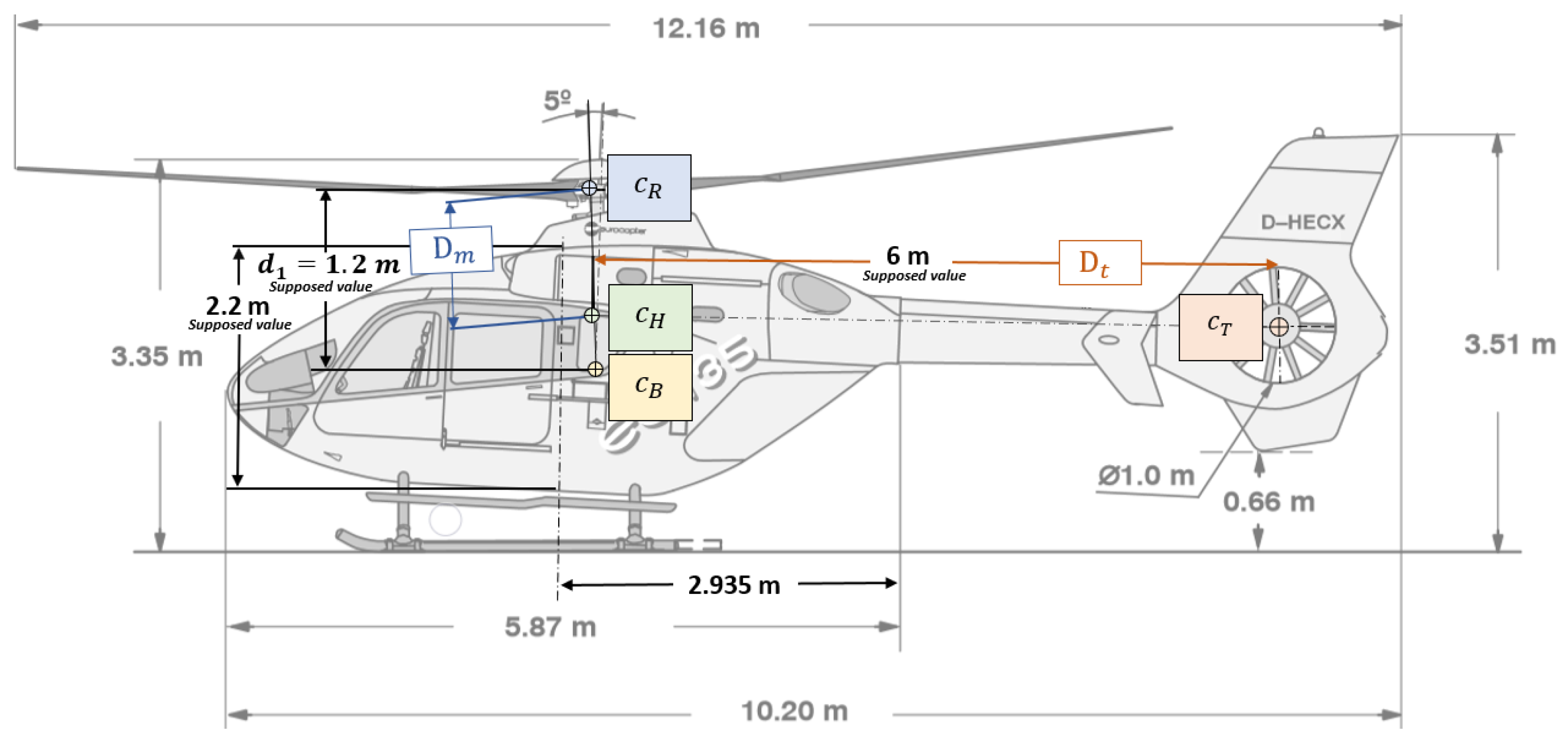
It is necessary to make some assumptions to calculate the center of mass of the helicopter and to determine the values $D_{\mathrm{m}}$ and $D_{\mathrm{t}}$. These assumptions refer to the Figure 8. It is assumed that the center of mass of the body $c_{\mathcal{B}}$ lies on the axis passing through the main rotor and perpendicular to the base. Furthermore, it is assumed that the center of mass of the main rotor $c_{\mathcal{R}}$ locates on an axis tilted 5 degrees from the vertical one. In addition, the main rotor and the body may be thought of as two objects composing the system $Body-MainRotor\left({}_{\mathcal{B},\mathcal{R}}\right)$, and the reference system for the calculation may be thought of as having the origin located in the point $c_{\mathcal{B}}$ and one axis that matches the axis tilted 5 degrees toward the point $c_{\mathcal{R}}$. We can determine the value of $c_{\mathcal{B},\mathcal{R}}$ by the equation

$$c_{\mathcal{B},\mathcal{R}}=\frac{Weigh{t}_{MainRotor}}{Weigh{t}_{MainRotor}+Weigh{t}_{Body}}·d_1.$$

(80)

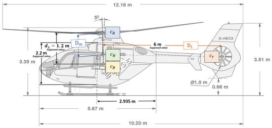
Figure 8. Values used to calculate the center of mass. (Figure adapted from [23], page 7.)

Now, assuming $d_1=1.2$ m as the distance between $c_{\mathcal{B}}$ and $c_{\mathcal{R}}$, the above equation gives

$$c_{\mathcal{B},\mathcal{R}}=\frac{277.2}{277.2+1134.6}·1.2\approx 0.235614\mathrm{m}.$$

(81)

Moreover, it is supposed that the contribution of the point $c_{\mathcal{T}}$ could be disregarded since the weight of the tail rotor is negligible compared to the fuselage weight and the main rotor weight; therefore, the tail rotor does not contribute to the calculations of the helicopter center of mass, hence it results $c_{\mathcal{B},\mathcal{R}}\approx c_{\mathcal{H}}$. The value of $D_{\mathrm{t}}\approx 6$ m has been inferred from the available data-sheets information and the structure drawings, and $D_{\mathrm{m}}$, that is the distance between the center of gravity of the helicopter and the main rotor, is $D_{\mathrm{m}}=d_1-c_{\mathcal{H}}\approx 0.964386$ m.

Features of the engines: The EC135 P2+ helicopter type is equipped with two PW206B2 engines from Pratt and Whitney Canada Corp^TM. To start engines there are two possibilities: manual control or automatic control. Manual control is not certificated and is normally deactivated. The automatic control is managed by the FADEC (Full Authority Digital Engine Control) that governs the starting procedure, the fuel flow and the RPMs automatically. At the start of the engines, the FADEC turns on the engines one by one until the RPMs reach the value of 98% ([1], page 437). When either the collective control or a manual switch are operated by the pilot, the FADEC increases the RPMs to 100% and the flight mode is engaged. When the altitude is higher than 4000 ft the speed is automatically increased to 104%, because the air density decreases. Moreover, to avoid loss of thrust when the collective angle is varied, in the main rotor (pitch) or in the tail rotor (yaw), the FADEC fixes the engine power to maintain the desired speed. The characteristics of the engines are summarized in Table 3.

Table 3. Values are taken from [25], pages 8 and 12. The helicopter state AEO denotes ‘all engine operative’, whereas the state OEI stands for ‘one engine inoperative’. Typically, two possible working mode could be selected: TOP (take-off power) that has a time-limit constraint, and MCP (maximum continuous power).

Engine Mode	Power	Maximum Torque
	[ kW ]	[ N · m ]
AEO TOP (max. 5 min)	2 × 333	2 × 519
AEO MCP	2 × 321	2 × 500
OEI (max. 30 s)	547	851
OEI (max. 2 min)	534	831
OEI MCP	404	629

Gear box: The gear box is a complex part that transmits power, usually reducing angular velocity and increasing torque. Both helicopter engines drive the gear box that, in turn, drives the main rotor shaft and the tail rotor shaft.

Main rotor thrust: The Equation (26) was used to calculate the power coefficient of the main rotor, that is $C_{\mathrm{w}}\approx 0.006968$, and its thrust coefficient $C_{\mathrm{u}}\approx 0.045965$. It is also possible to determine the maximum thrust $u_{\mathrm{m},\max }$ generated by the main rotor using the Equation (24), setting the throttle at 100% and the collective angle at its maximum. The obtained result is $u_{\mathrm{m},\max }\approx \mathrm{52,729}\frac{\mathrm{kg}·\mathrm{m}·{\mathrm{rad}}^2}{{\mathrm{s}}^2}.$ Such numerical result was obtained by setting ${\mathsf{\Omega }}_{\mathrm{m},max}\approx 41.364303$ rad/s, ${\alpha }_{\mathrm{c},\max }=0.541052$ rad, $\rho =1.225$ kg/m${}^3$ (which denotes, respectively, the maximum angular speed, the maximum collective angle and the air density at 15 Celsius degrees and 1 atm, from Table 1).

Tail rotor thrust: In the same way, it is possible to determine the power coefficient and the thrust coefficient for the tail rotor which are respectively $C_{\mathrm{w}}^{\mathrm{T}}\approx 0.100974$ and $C_{\mathrm{u}}^{\mathrm{T}}\approx 0.273201$. The maximum thrust generated by the tail rotor is $u_{\mathrm{t},\max }\approx 2601\mathrm{kg}·\mathrm{m}·{\mathrm{rad}}^2/{\mathrm{s}}^2$, whose value is calculated using the throttle at 100%, the angular velocity ${\mathsf{\Omega }}_{\mathrm{t},max}\approx 375.315601$ rad/s and the maximum collective angle for the tail rotor ${\alpha }_{\mathrm{c},\max }^{\mathrm{T}}\approx 0.596903$ rad, from Table 1.

Drag term: According to Equation (28), the value of the drag term is $\gamma \approx 0.154546$$\mathrm{m}$. Such numerical result was obtained by setting the middle value of the interval of the tail rotor collective angle to ${\alpha }_{\mathrm{c},\mathrm{mid}}^{\mathrm{T}}\approx 0.151844$ rad, and the collective angle of the main rotor consistent with hovering to ${\alpha }_{\mathrm{c},\mathrm{hover}}\approx 0.268693$ rad, from Equation (69).

Friction terms: Let us collect the tip velocity of the helicopter along each axis in the vector ${\dot{p}}_{\max }$. Given the maximum velocity of the helicopter, we know that, once reached that particular value, the acceleration of the helicopter along that axis will drop to 0, because of the existence of a friction force in the opposite direction. This situation can be described as:

$$\begin{array}{c}0=R({\phi }_{\mathrm{m}}+{\phi }_{\mathrm{t}})-M_{\mathcal{H}}\overline{g}{e}_{\mathrm{z}}-B{\dot{p}}_{\max }.\hfill \end{array}$$

(82)

Looking closely at the term $R({\phi }_{\mathrm{m}}+{\phi }_{\mathrm{t}})$, namely the propelling force of the helicopter, it is readily observed how it takes a special configuration when the tip speed is reached, in fact:

• To reach the tip speed along the z-axis, it is necessary that the z-axes of the inertial reference frame ${\mathcal{F}}_E$ and of the body-fixed reference ${\mathcal{F}}_B$ are aligned;
• To reach the tip speed along the x-axis, we consider a motion at maximum speed due to a total thrust directed along the x-axis while in a horizontal attitude ($R=I_3$). In this case, the thrust takes its maximum value (compatibly with the need to keep the helicopter hovering).

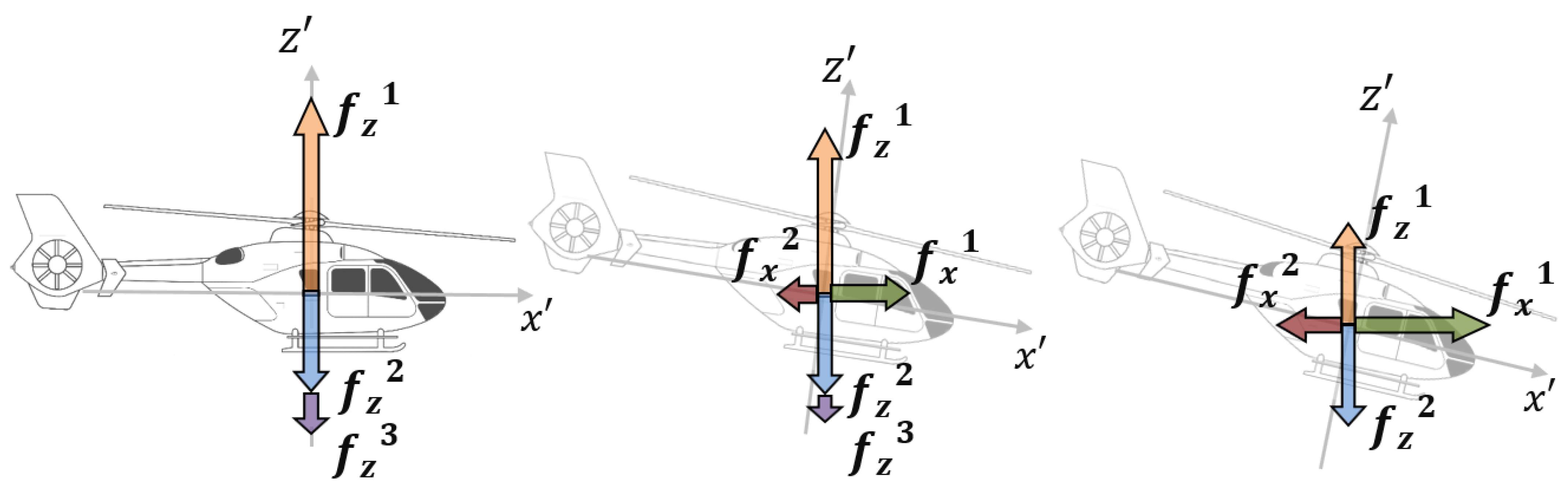
The Figure 9 shows the force components present in some particular helicopter attitudes. In the frame on the left-hand side of the figure, the helicopter is horizontal, namely $R=I_3$, and all the forces are directed along the z-axis, disregarding the force exerted by the tail rotor. In the frame on the right-hand side, the helicopter is in a hovering condition, therefore, the friction force $F_{\mathrm{z}}^3=0$, while the friction force $F_{\mathrm{x}}^2$ along the x-axis is maximum.

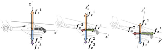
Figure 9. Friction terms encountered by a flying helicopter in correspondence of an increasing horizontal speed. The variables are defined as $f_{\mathrm{z}}^1=e_{\mathrm{z}}^{\top }\phi ,f_{\mathrm{z}}^2=M_{\mathcal{H}}\overline{g},f_{\mathrm{z}}^3=e_{\mathrm{z}}^{\top }\dot{p}{\beta }_{\mathrm{v}},f_{\mathrm{x}}^1=e_{\mathrm{x}}^{\top }\phi ,f_{\mathrm{x}}^2=e_{\mathrm{x}}^{\top }\dot{p}{\beta }_{\mathrm{h}}$.

The friction terms were calculated upon determining the tip speed of the helicopter. For the EC135 P2+ helicopter, the found values are summarized in Table 4. Since we only know the maximum linear speed along the x-axis, we consider as null the friction force along the y-axis.

Table 4. Airspeed value ([24], page 23). Hover turning velocity and throttle range ([23], pages 43 and 35). Rate of climbing (page 60 in [26]).

Limit Values				Condition
	[$\mathbf{m}/\mathbf{s}$]	[$\mathbf{rad}/\mathbf{s}$]	$\mathbf{min}÷\mathbf{max}$ [%]
Airspeed	79.7	−	−	Sea level, +20 Celsius degrees, gross mass up to 2300 kg, TOP mode
Rate of climbing	8.9	−	−
Hover turning	−	1.047	−
Throttle range	−	−	97 ÷ 104

Using the Equation (82) and the speed limit values, it is possible to infer the values of the coefficients ${\beta }_{\mathrm{h}}$ and ${\beta }_{\mathrm{v}}$, namely the friction term along the x-axis and the z-axis, respectively. The vector of the maximum speed reads ${\dot{p}}_{\max }={[79.7?8.9]}^{\top }$, referring to the Table 4. In addition, we considered the result from (71) and we end up with an equation depending on the unknown coefficient ${\beta }_{\mathrm{h}}$, where the other terms are known:

$$2{\beta }_{\mathrm{h}}{e}_{\mathrm{x}}^{\top }{\dot{p}}_{\max }=u_{\mathrm{m},\max }sin\left(\arccos \left(\frac{2M_{\mathcal{H}}\overline{g}}{u_{\mathrm{m},\max }}\right)\right),$$

(83)

where $e_{\mathrm{x}}:={\left[100\right]}^{\top }$. The Equation (83) allows to infer the value of the friction term.

The term $\arccos \left(\frac{2M_{\mathcal{H}}\overline{g}}{u_{\mathrm{m},\max }}\right)\approx 58$ deg describes the angle with respect to the x-axis of the inertial reference frame ${\mathcal{F}}_E$ that the total thrust $\phi$ must take for the helicopter to reach the maximum velocity. The orientation of the thrust $\phi$ can be managed by the pilot by operating the cyclic control, which varies the angles ${\alpha }_{\mathrm{p}}$ and ${\alpha }_{\mathrm{r}}$, and by controlling the helicopter’s overall attitude R.

To determine friction coefficients, the hover condition is preserved and rolling and pitching are not involved. The friction term ${\beta }_{\mathrm{v}}$ can be determined by fixing ${\alpha }_{\mathrm{p}}=0$, ${\alpha }_{\mathrm{r}}=0$ and $R=\mathrm{diag}(1,1,1)$, which are the conditions to reach the maximum velocity along the z-axis. From the Equation (82), we thus obtain

$${\beta }_{\mathrm{v}}{e}_{\mathrm{z}}^{\top }{\dot{p}}_{\max }=\frac{1}{2}{u}_{\mathrm{m},\max }-M_{\mathcal{H}}\overline{g}.$$

(84)

Instantiating equations (83) and (84) with known values, the friction coefficients can be easily computed. It has been found that ${\beta }_{\mathrm{h}}\approx 281$ kg·s${}^{-1}$ and ${\beta }_{\mathrm{v}}\approx 1398$ kg·s${}^{-1}$.

Using the same method, it is possible to estimate the value of ${\beta }_{\mathrm{r}}$, the friction term linked to the yaw velocity. Let us assume the helicopter to be in the hovering condition, with ${\dot{\xi }}_{\mathrm{m}}={\dot{\xi }}_{\mathrm{t}}=0$. At the maximum yaw speed the angular acceleration will be null. Since we consider a hovering condition with ${\alpha }_{\mathrm{r}}={\alpha }_{\mathrm{p}}=0$, the total torque $\tau$ is equal to $\frac{1}{2}(D_{\mathrm{t}}{u}_{\mathrm{t},\max }-\gamma u_{\mathrm{m},\mathrm{hover}}){\xi }_z$; therefore, from the second equation in (66) we obtain $0=S^{-1}([{\widehat{J}}_{\mathcal{H}}^{\star },{\xi }_{\max }^2]+\left(D_{\mathrm{t}}{u}_{\mathrm{t},\max }-2\gamma M_{\mathcal{H}}\overline{g}-{\beta }_{\mathrm{r}}⟨{\xi }_{\max },{\xi }_z⟩\right){\xi }_z)S^{-1}$, where ${\xi }_{\max }$ denotes the maximal yawing speed that, from the Table 4, is known to be ${\xi }_{\max }=1.047·{\xi }_z$ (rad/s). Thus, isolating the friction term, this equation becomes:

$${\beta }_{\mathrm{r}}⟨{\xi }_{\max },{\xi }_z⟩{\xi }_z=[{\widehat{J}}_{\mathcal{H}}^{\star },{\xi }_{\max }^2]+\left(D_{\mathrm{t}}{u}_{\mathrm{t},\max }-2\gamma M_{\mathcal{H}}\overline{g}\right){\xi }_z.$$

(85)

To determine the correct value of the friction term it is necessary to fill the Equation (85), namely the tip thrust of the tail rotor $u_{\mathrm{t},\max }$, the structural values, and the drag coefficient found. The computed result for this parameter is ${\beta }_{\mathrm{r}}\approx 10797$ N·m·s·rad${}^{-1}$.

6. Numerical Experiments and Results

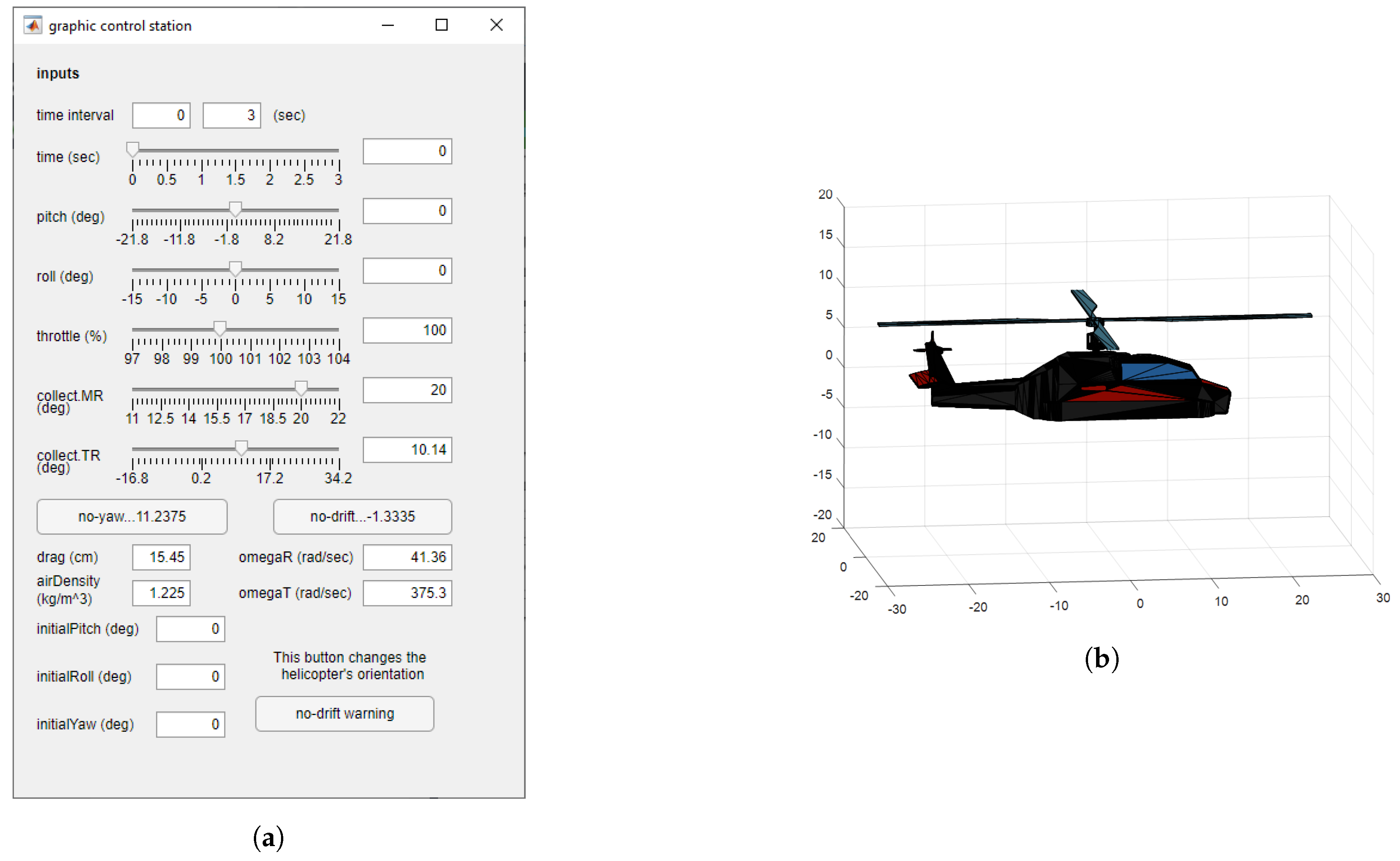
A series of tests of the mathematical model were carried out by means of a MATLAB^® implementation of the numerical methods explained in Section 4. In order to clarify what can be tested, and how, it could be useful to introduce the graphic control panel shown in Figure 10.

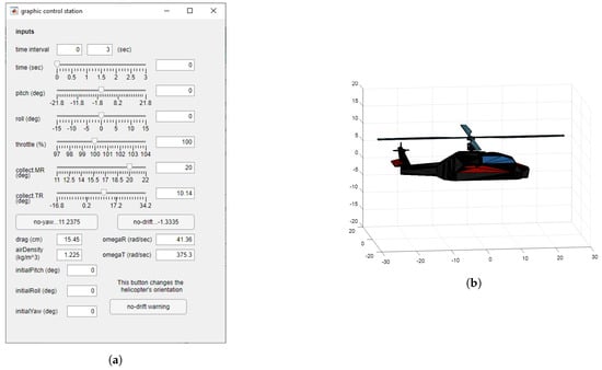
Figure 10. Graphic input interface: (a) graphic interface used to test the model; (b) graphic window to show the initial attitude of the helicopter, which is linked to the value of the matrix R selected.

The cell time interval allows to set the time range for new experiments. The interface gives the possibility to perform series of test, therefore, the initial value of time interval could not be set at an instant of time $t_1$ until another experiment, which ended at $t_1$, has been completed. The slider named Time shows the selected instant of time in a pop-up animation window. Every slider is linked to an editable cell, hence, any value belonging to the correct range could be directly set. The five sliders pitch, roll, throttle, collect.MR, collect.TR are the interface to manage the value of the variables ${\alpha }_{\mathrm{p}},{\alpha }_{\mathrm{r}},{\mathsf{\Omega }}_{\mathrm{m}},{\alpha }_{\mathrm{c}},{\alpha }_{\mathrm{c}}^{\mathrm{T}}$, respectively. The no-yaw button sets the angle ${\alpha }_{\mathrm{c}}^{\mathrm{T}}$ for a no-yawing condition, from Equation (72), whereas the button no-drift manages the value of the angle ${\alpha }_{\mathrm{r}}$ to achieve a no-drifting condition using the Equation (73). The two editable cells drag and air density allow to input the values of the coefficients $\gamma$ and $\rho$, respectively. The three cells initial roll, initial pitch, initial yaw interface with the matrix R forcing a value of attitude of the helicopter along the three axes $x,y,z$. The button no-drift warning changes the initial roll value in order to achieve a stationary no-drifting condition (a technique introduced in the third test).

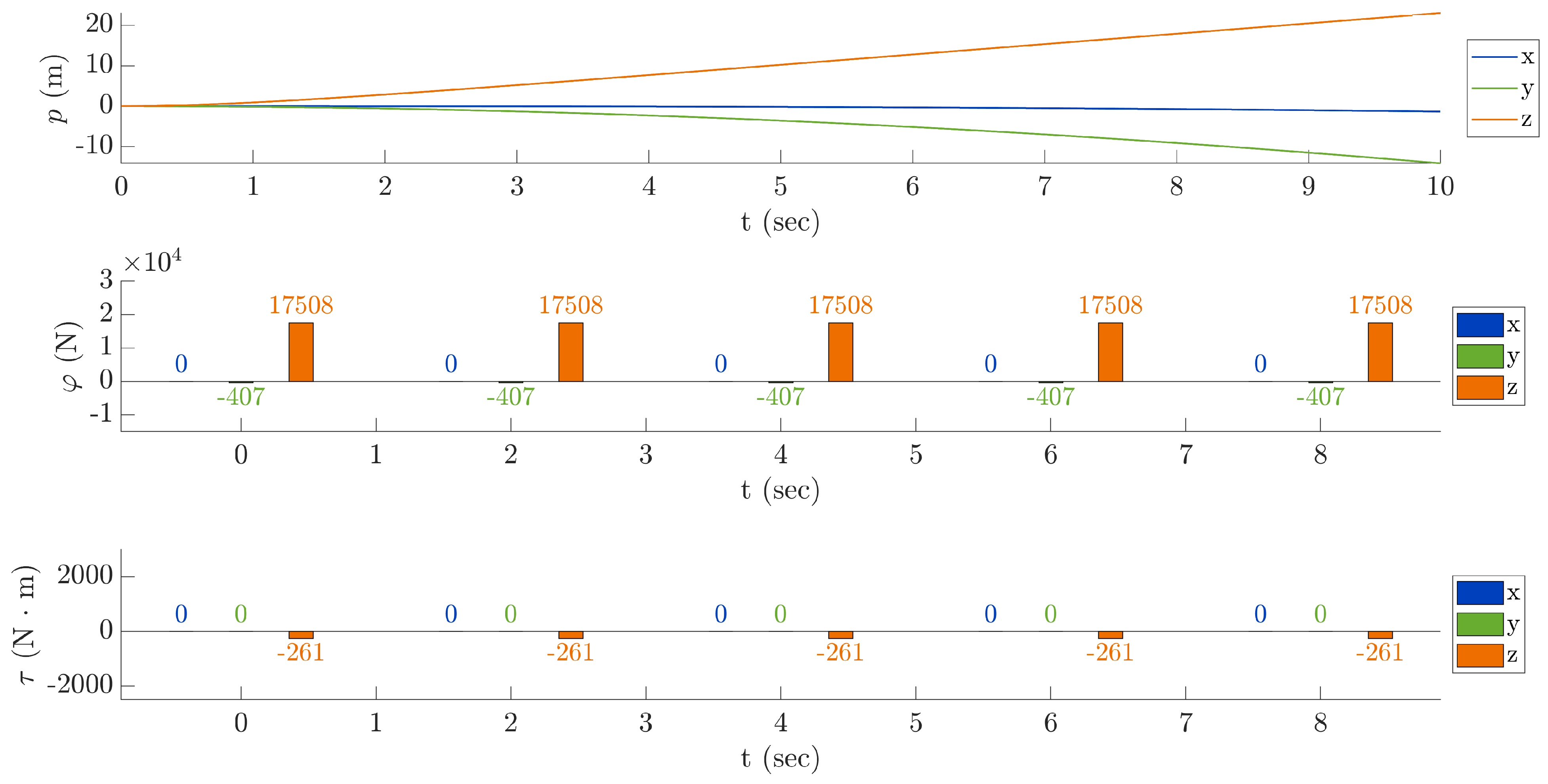
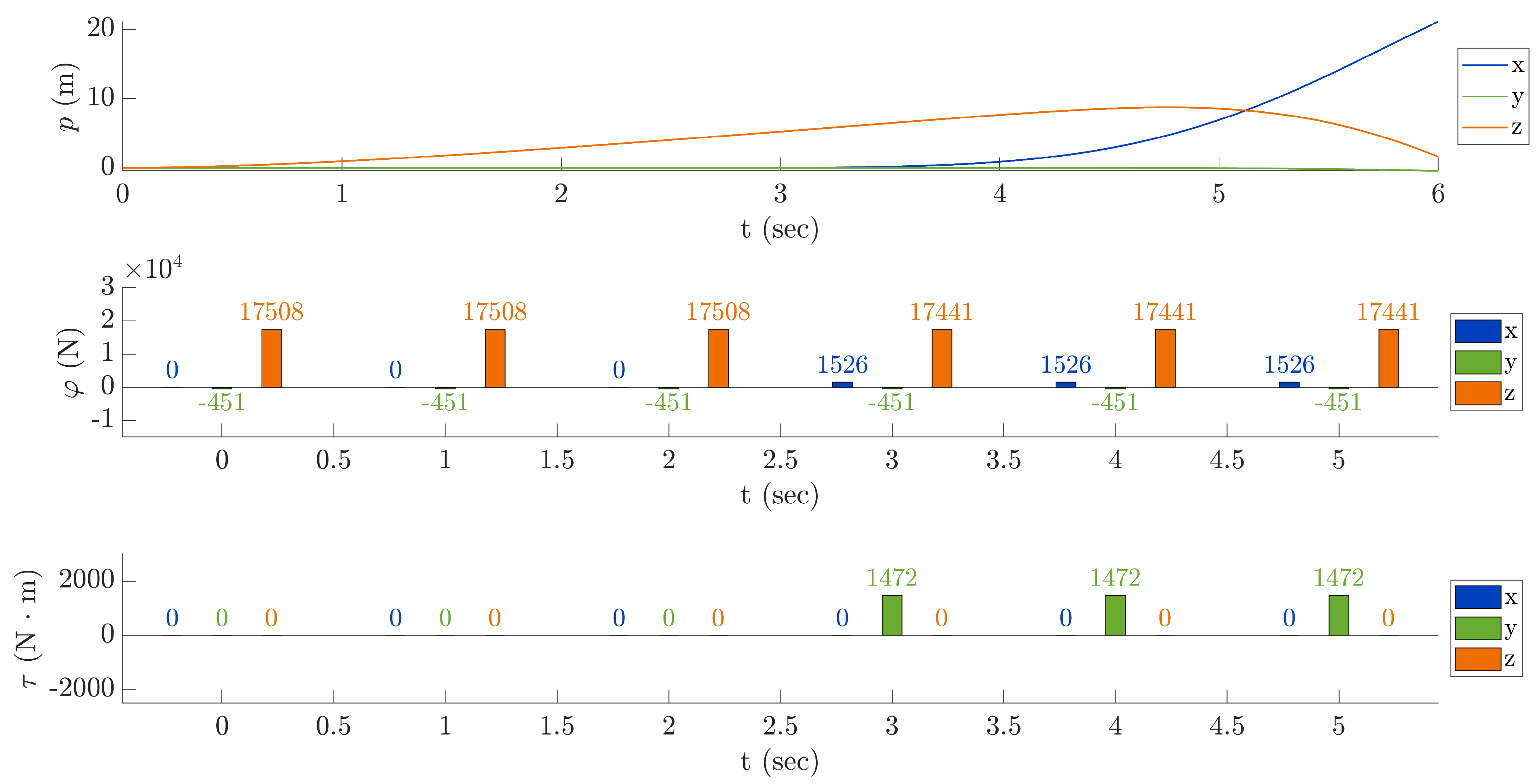
First test—lift response: The first test lasts 10 s and does not involve pitch and roll angles (${\alpha }_{\mathrm{p}}=0$, ${\alpha }_{\mathrm{r}}=0$), moreover the throttle is set at $100\%$ and the tail rotor collective angle at ${\alpha }_{\mathrm{c},\mathrm{mid}}^{\mathrm{T}}$. About the main rotor collective angle, it has been chosen in order to produce lift along z-axis: the value chosen is 20 degrees. Figure 11 shows the result of this simulation. The position along x-axis is constant, which could seem reasonable because pitch angle is not involved. On the other hand, there is a clear decrease in the y-component of the positional variable p due to drift effect. Notice that the direction of the tail rotor thrust is opposite to y-axis, as Figure 5 shows. The z component of the torque $\tau$ is negative, and this is the cause of clockwise yawing. Looking closely at the entries of the position vector p, along the x-axis it can be observed a little decrease due to the combined action of the helicopter yawing and tail rotor drift. In fact, when the helicopter nose turns, the drift effect causes a slight decrease in the positional x-coordinate. Note that the drift force exerted by the tail rotor coincides with the y component of the total thrust $\phi$, which is $e_{\mathrm{y}}^{\top }\phi$. The last remarkable observation from the first test is that the z component of the thrust $\phi$ has the value of $\mathrm{16,191}$ N, which is more than the helicopter-weight force, that could be determined from Table 2 as $1420·\overline{g}\approx \mathrm{13,925}$ N. The resulting force along the z-axis is positive and, as described by the graph of the z-coordinate of the center of gravity, the helicopter lifts up.

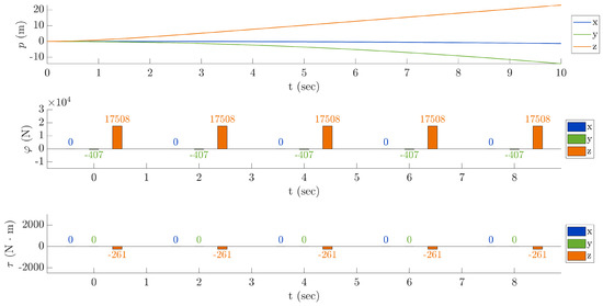
Figure 11. First test—lift response. Top panel: components of the position of $c_{\mathcal{H}}$. Middle panel: components of the thrust. Bottom panel: components of the active torque generated by rotors.

Remark: The x, y and z components in the torque graph have been extracted from the Equation (14) following the construction of $\tau$, namely they are calculated by $e_{\mathrm{z}}^{\top }\tau e_{\mathrm{y}}$, $e_{\mathrm{x}}^{\top }\tau e_{\mathrm{z}}$ and $e_{\mathrm{y}}^{\top }\tau e_{\mathrm{x}}$.

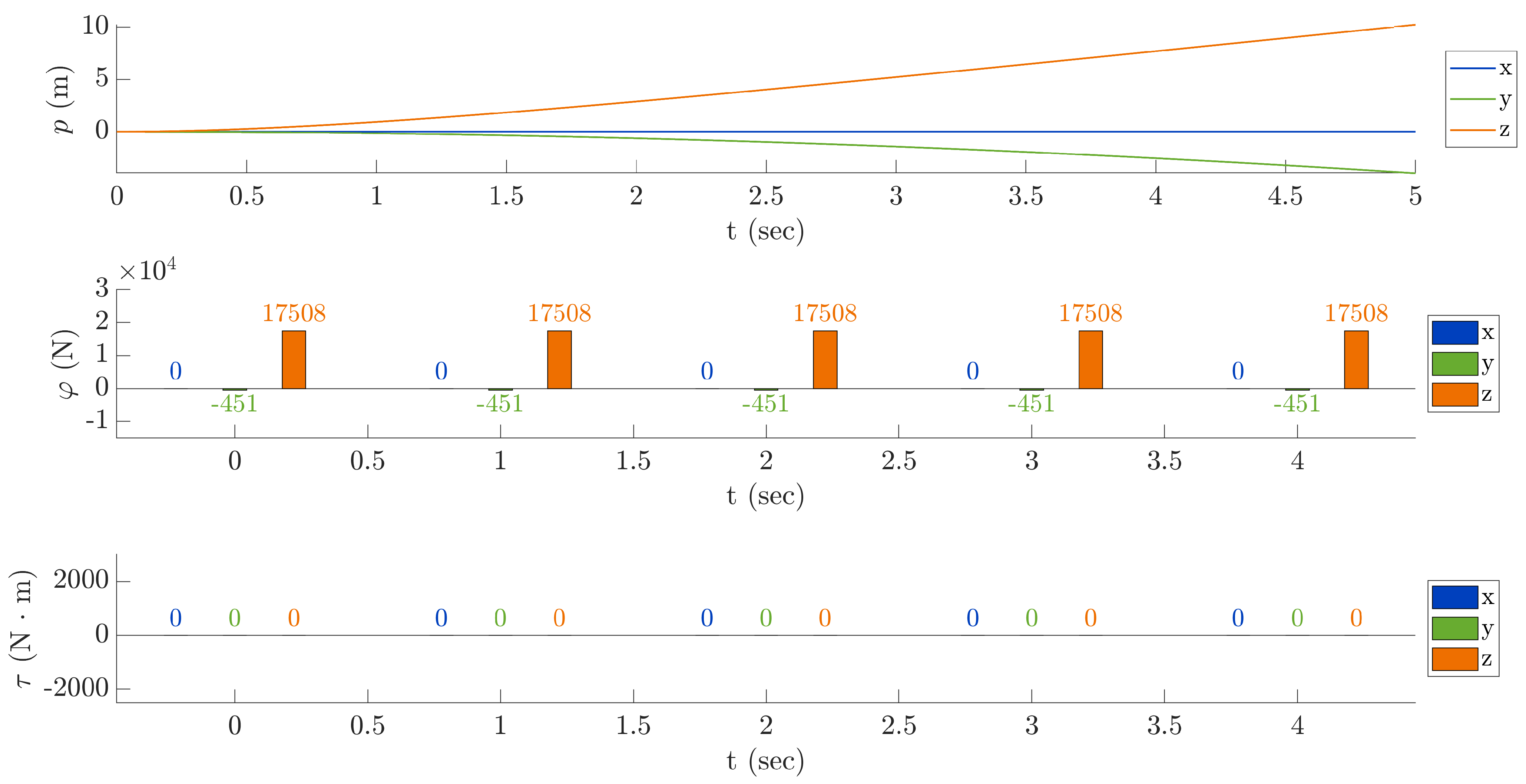
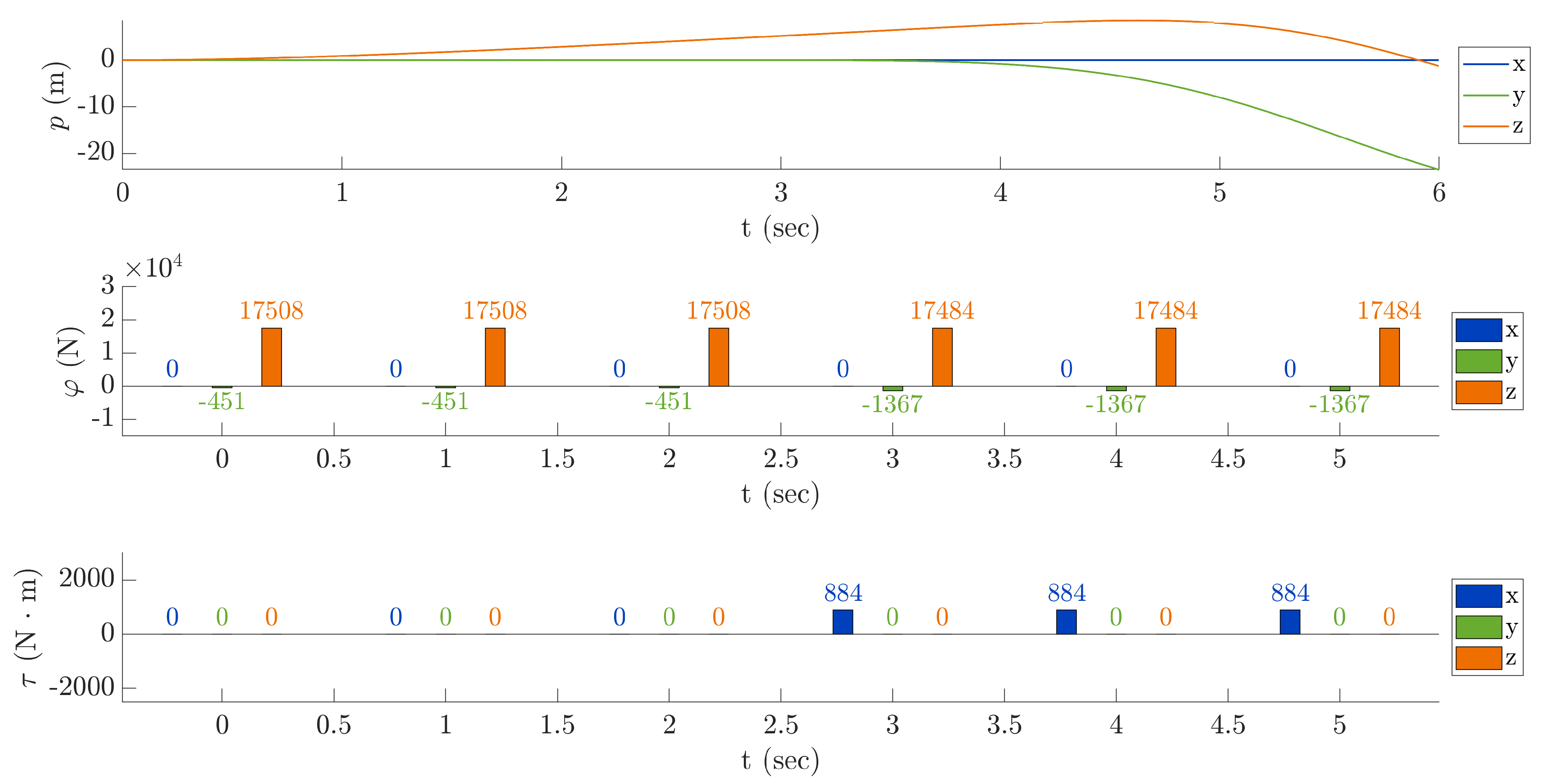
Second test—no yaw: This simulation lasts 5 s and illustrates how to select the tail rotor collective angle using the Equation (72) to achieve a no-yawing condition. From the graph of the torque $\tau$ it is clear that the torque exerted on the helicopter becomes null. Consequently, the slight decrease in the position along the x-axis, which was a side effect of the yawing, is no more present. The result is presented in Figure 12.

Figure 12. Second test—no yaw.

Third test—neither yaw nor drift: The third test illustrates the suppression of the drift effect due to the tail rotor. In this case, the y coordinate of the center of gravity of the helicopter does not vary, since the helicopter’s attitude is modified by using the no-drift warning button in the control graphic panel. Such function does not cause a change in the angle of attack of the blades as in the previous test, but in the initial roll angle and, as a consequence, in the matrix R. In fact, the helicopter’s attitude is set according to the Equation (73) along the x-axis, and such rotation produces an equilibrium among the drift effect and the thrust along the y-axis. The equilibrium among the forces causes the y-coordinate to stay constant, as wanted. The no-drift attitude is computed through the relation

$$R^{\star }:=\left[\begin{array}{ccc}1& 0& 0\\ 0& cos({\alpha }_{\mathrm{noDrift}})& -sin({\alpha }_{\mathrm{noDrift}})\\ 0& sin({\alpha }_{\mathrm{noDrift}})& cos({\alpha }_{\mathrm{noDrift}})\end{array}\right].$$

The result of this experiment is shown in Figure 13. As expected, only the z coordinate of the helicopter varies over time.

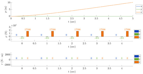
Figure 13. Third test—neither yaw nor drift.

The following tests were performed starting from the result of the third test, namely from a no yaw/no drift condition; therefore, the first 3 s of the results of each tests will be common to every execution.

Fourth test—pitch response: The fourth test is about pitch response. The pitch angle has been set to 5 degrees (constant) starting from the third second of the simulation to the end. In the result, illustrated in Figure 14, it can be seen an increase in the y-component of the total mechanical torque $\tau$. It is also possible to notice, as Figure 9 shows, that the change in the angle ${\alpha }_{\mathrm{p}}$ causes a variation in the $\phi$ components. Indeed, the x component of the total thrust $\phi$, that is $e_{\mathrm{x}}^{\top }\phi =\frac{1}{2}{u}_{\mathrm{m}}sin{\alpha }_{\mathrm{p}}cos{\alpha }_{\mathrm{r}}$, increases as ${\alpha }_{\mathrm{p}}$ increases, whereas the z component of $\phi$, that is $e_{\mathrm{z}}^{\top }\phi =\frac{1}{2}{u}_{\mathrm{m}}cos{\alpha }_{\mathrm{p}}cos{\alpha }_{\mathrm{r}}$, decreases as ${\alpha }_{\mathrm{p}}$ increases.

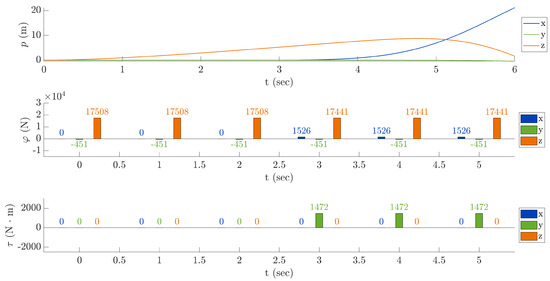
Figure 14. Fourth test—pitch response.

Fifth test—positive roll response: In this test, we set the angle ${\alpha }_{\mathrm{r}}$ from the third second to the sixth second to 3 degrees. The obtained result is presented in Figure 15 and shows an increase in the x component of the mechanical torque $\tau$. This behavior follows the Equation (66), where ${\alpha }_{\mathrm{r}}$ is linked to the x component of the mechanical torque $\tau$. In addition, using the same equation it is immediate to see that the y component of $\tau$ is zero because ${\alpha }_{\mathrm{p}}=0$. Let us remark that instead the z component of $\tau$ is zero because of the no-yaw condition.

Figure 15. Fifth test—positive roll response.

As in the previous example, a change of the angle ${\alpha }_{\mathrm{r}}$ causes the z component of the thrust vector $\phi$ to decrease. Moreover, the magnitude of the y component of the vector $\phi$ increases and adds up to the drifting effect of the tail rotor. It is important to point out, from the graph of the components of the positional vector p, that rolling causes a falling situation, as well as a shift along the y-axis.

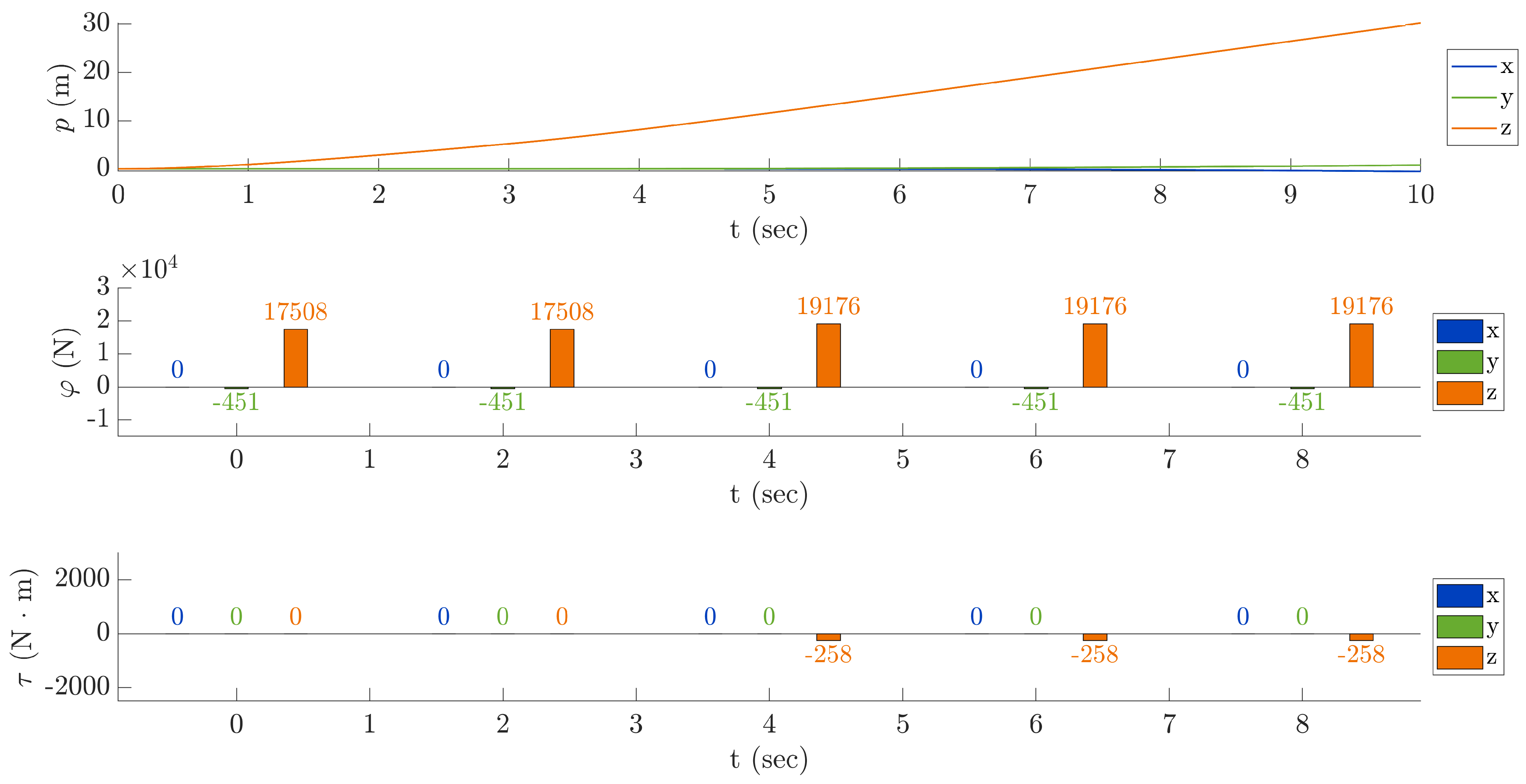
Sixth test—main rotor collective response: The collective control is amply used for managing the acceleration of the helicopter. The test of this specific control system has been made increasing up to 22 degrees the main rotor collective angle starting from the third second to the tenth second. The increase in the main rotor collective angle causes a thrust boost, which increases the lifting of the helicopter. The result is shown in Figure 16. As remarked, every time collective control is operated the helicopter pilot also has to adjust the tail rotor collective angle, since the no-yaw flight mode depends on $u_{\mathrm{m}}$, which is a function of ${\alpha }_{\mathrm{c}}$. This side effect could be observed from the values of the z component of the mechanical torque $\tau$ whose magnitude changes and needs to be adjusted through the pedals control.

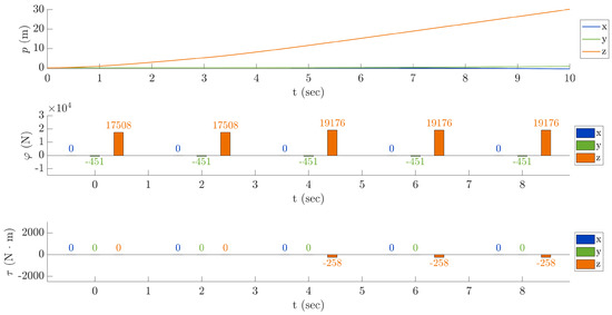
Figure 16. Sixth test—Main rotor collective response.

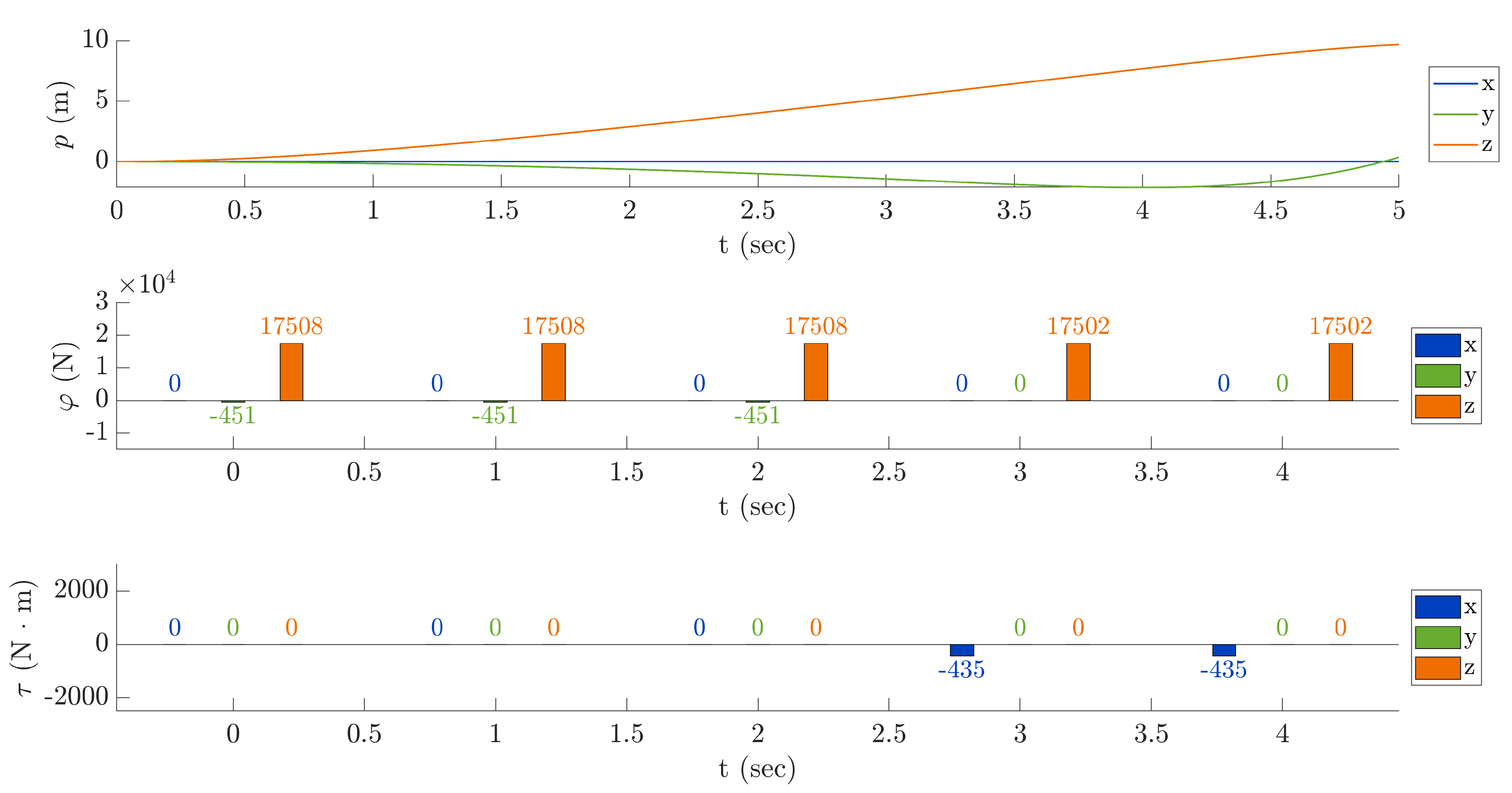
Seventh test—negative roll response: The Figure 17 shows results of a test in which it has been tried to remove the drift effect using the cyclic control. It has already been remarked that a force control is not sufficient to remove the drift effect, since a combined helicopter’s attitude control is needed. The no-drift flight mode could be achieved, for example, using a PID control on the helicopter’s attitude.

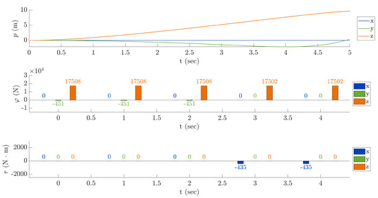
Figure 17. Seventh test—negative roll response.

This test was carried out using as initial setting the same setting as for the second test, whereas the last 2 s were simulated using the Equation (73) to change ${\alpha }_{\mathrm{r}}$. Notice that an attitude controller would ensure no drifting. Ideally, a PID controller should reduce the value of the cyclic control as the roll angle of the helicopter approaches the value determined by the Equation (73).

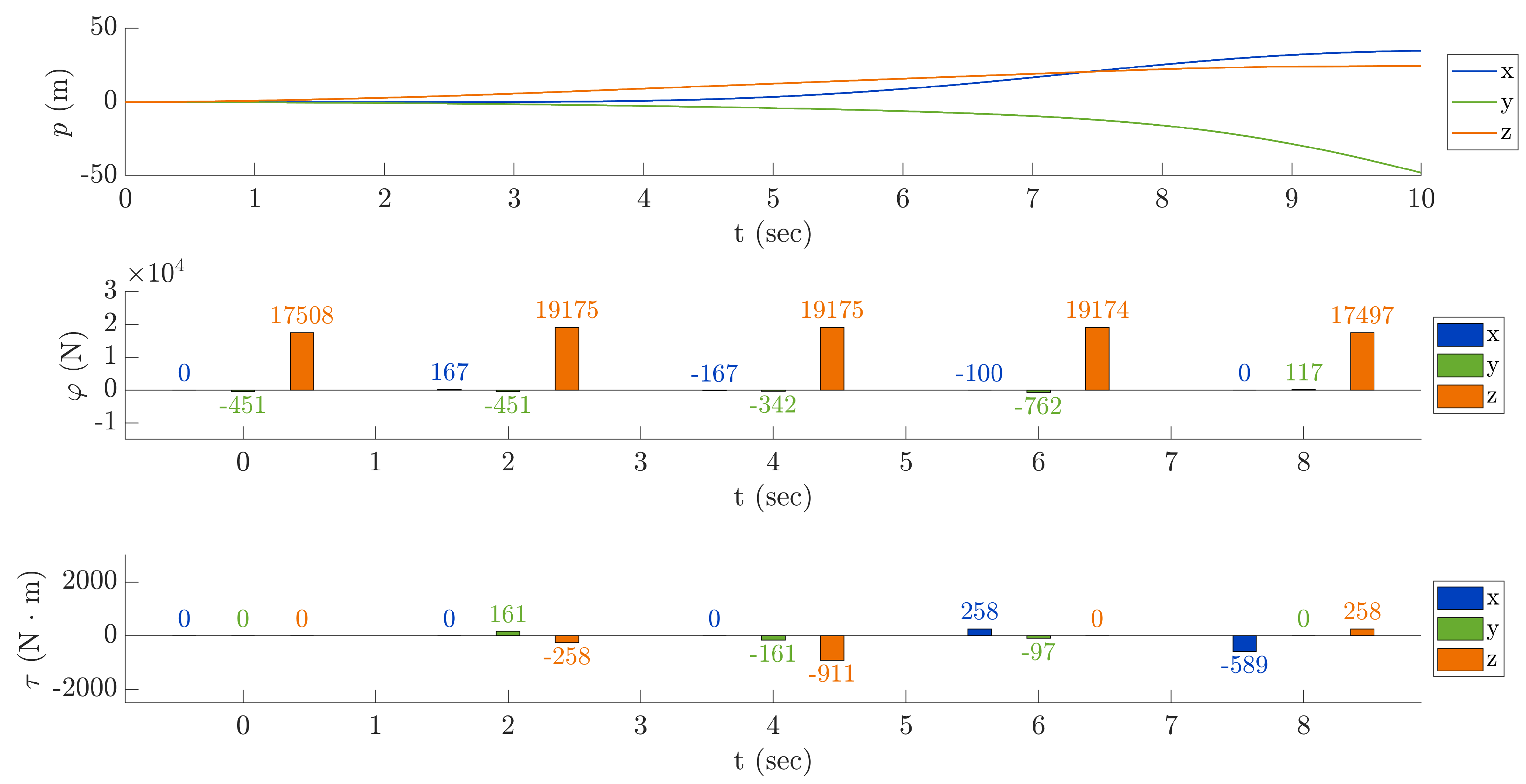
Eight test—free flight: This last test consists in a simulation of a free flight achieved by setting multiple inputs for the cyclic control and the collective control. The obtained result is shown in Figure 18, while Table 5 presents the time line of the controls used. The throttle during the test keeps constant to 100%. The results of this simulation is exemplified by a video attached to the present paper as a supplemental material.

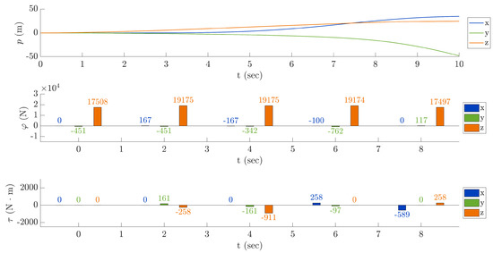
Figure 18. Eighth test—free flight.

Table 5. Eighth test—free flight. The orange-colored values indicate that the no-yaw flight mode has been activated in that time window.

Time Line of Controls
Time Interval	(s)	[0–2)	[2–4)	[4–6)	[6–8)	[8–10]
${\alpha }_{\mathrm{p}}$	(deg)	0	0.5	$-0.5$	$-0.3$	0
${\alpha }_{\mathrm{r}}$	(deg)	0	0	0	0.8	$-2$
${\alpha }_{\mathrm{c}}$	(deg)	20	22	22	22	20
${\alpha }_{\mathrm{c}}^{\mathrm{T}}$	(deg)	11.24	11.24	8.5	12.32	12.32

A visual animation of the flight trajectory obtained in this test is available.

7. Conclusions

The aim of this paper was to devise a mathematical model of a fantail helicopter in the framework of Lie-group theory. The main theoretical instrument, besides of Lie-group theory itself, is the Lagrange–d’Alembert–Pontryagin principle, which generalizes the Lagrangian formulation of dynamics to curved manifolds and to dissipative systems.

The modeling endeavor resulted in a series of differential equations, two of which describe the rotational dynamics of the helicopter body and two describe its translational dynamics. The terms in the equation have been analyzed to link the abstract mathematical notation with the physics of the real-world system under examination. In addition, a number of specific equations to calculate thrusts and power factors have been presented and merged to the Lie-group equations.

A specific section of the paper dealt with the numerical simulation of the flight of a helicopter and explained a specific numerical method to solve Lie-group-type differential equations approximately yet keeping up with the intrinsic nature of the base Lie-group (namely, the space of three-dimensional rotations).

The equations that compose the devised helicopter model include a number of parameters whose values are necessary to perform actual numerical simulations. Since most of such values are not directly available in the literature, a careful work of identification of the parameters through the devised equations has been carried out.

Numerical results have been illustrated and commented in order to elucidate some aspects of the model that were deemed of particular interest, from simple flight modes to free flight. The devised model, as the large majority of mathematical models of real-world physical phenomena, is of potential use to control engineers (who may use such mathematical model to design a state observer and an automatic control system to assist the pilot), to mechanical engineers (who may use the devised model to test a helicopter structure under stress conditions) and by pilots instructing facilities (who might use the devised model as a prototypical flight simulator).