Reliability Simulation of Two Component Warm-Standby System with Repair, Switching, and Back-Switching Failures under Three Aging Assumptions

Abstract

We analyze the influence of repair on a two-component warm-standby system with switching and back-switching failures. The repair of the primary component follows a minimal process, i.e., it experiences full aging during the repair. The backup component operates only while the primary component is being repaired, but it can also fail in standby, in which case there will be no repair for the backup component (as there is no indication of the failure). Four types of system failures are investigated: both components fail to operate in a different order or one of two types of switching failures occur. The reliability behavior of the system is investigated under three different aging assumptions for the backup component during warm-standby: full aging, no aging, and partial aging. Four failure and repair distributions determine the reliability behavior of the system. We analyzed two cases—in the First Case, we utilized constant failure rate distributions. In the Second Case, we applied the more realistic time-dependent failure rates. We used three methods to identify the reliability characteristics of the system: analytical, numerical, and simulational. The analytical approach is limited and only viable for constant failure rate distributions i.e., the First Case. The numerical method integrates simultaneous Algebraic Differential Equations. It produces a solution in the First Case under any type of aging, and in the Second Case but only under the assumption of full aging in warm-standby. On the other hand, the developed simulation algorithms produce solutions for any set of distributions (i.e., the First Case and the Second Case) under any of the three aging assumptions for the backup component in standby. The simulation solution is quantitively verified by comparison with the other two methods, and qualitatively verified by comparing the solutions under the three aging assumptions. It is numerically proven that the full aging and no aging solutions could serve as bounds of the partial aging case even when the precise mechanism of partial aging is unknown.

1. Introduction

Assessing the reliability of a system is a key engineering task that has economic and safety implications. Having a better understanding of failure/repair rates of system components is a tool to design highly reliable systems and conduct repair operations at adequate cost levels while complying with adequate and reasonable maintenance schedules. A common approach for improving the reliability is to provide redundancy for excessively failing components. The redundant components may operate simultaneously in a sense that the system will never fail if at least one of the parallel components operates [1]. Another possibility is to design a “k out of n” configuration where all n components are in operation and the system is not failing if at least k of them operate properly [2]. However, the standby arrangement is the simplest, cheapest and the most utilized one; the system operates with some of its components (called primary) whereas the redundant components (called backup components) are in standby, but when a primary component fails, they take its place [3]. In this paper, we will focus on a two-component system with a standby arrangement where the backup components may fail either while in standby, or during operation after some imperfect switching mechanism has put those online. The switching mechanism can be continuous type when it actively monitors the primary component and makes its own decisions, but it can malfunction at any time [4]. However, in this paper, we will treat exclusively the widespread mechanisms that can fail only on demand when the switching is needed [5]. According to the failure intensities of the backup component, such systems are classified as cold-standby, warm-standby, and hot-standby [6]. In the hot-standby system, the intensity of failures of the backup component is the same during standby and operation, whereas in the cold-standby, there is no failure in standby. We will concentrate on the two-component warm-standby systems where there are failures of the backup component in standby, but with smaller intensity compared to its operational mode.

Additionally, the reliability of a system with backup components depends on the way of aging of the backup components while in standby. Previous works have identified three types of aging of the backup component during warm-standby: full aging, no aging and partial aging [7]. The full aging assumption means that the component changes its failure/repair rate during standby as if it is operational. Under the no aging assumption, the component does not change its failure/repair rate during standby. The partial aging assumption models the intermediate situation where the backup component experiences some wear during standby, but at a slower rate than if operational.

If some components of the system are deemed repairable, the system can be brought to its full operational capacity by replacing parts or by making adjustments [8]. In most works, the focus is on single-component repairable systems under various repair activities. A detailed discussion on how such tasks can be approached with modern statistical tools is offered in [9]. There are different types of repairs that can be adopted depending on objectives. The first possibility is the so-called perfect repair (a.k.a. as-good-as-new (AGAN) repair), where the primary component fails and it is replaced or restored to its original or good-as-new condition [10]. Minimal repair restores the device to the condition it was in immediately before the failure [11] (pp. 226–227). There may also be intermediate types of repairs (e.g., the partial perfect repair procedures mentioned in [8]). In the current work, the focus is on the case of minimal repair of the special type worse-than-old (WTO) [12]. The assumption is that during this repair, the non-repaired elements of the primary unit age as if the latter was operational.

In this paper, we will investigate the effects that adding repair and back-switching failures to a two-component warm-standby system with switching mechanism has on the reliability of the system. Our goal is to analyze how this affects the system reliability under different aging assumptions in standby. In such a system, the primary component begins operation, and when it fails, the system will try to activate the backup component, but a switching failure is possible. When the backup component is operational, the primary component undergoes minimal repair. If the latter finishes before the backup component fails, the system will try to activate back the primary component, but again a back-switching failure is possible. However, it is possible that the backup component will fail in standby. In that case, there will be no repair for the backup component since there will be no indication of the failure. The system is considered to have failed when either both components fail to operate at any given time, or when, after primary component failure, the switching mechanism fails on demand to switch the system operation to the secondary component (switching failure), or when, after a successful repair, the switching mechanism fails on demand to switch the system operation back to the primary component (back-switching failure). The primary component undergoes minimal repair, i.e., the primary component experiences full aging during the repair. The reliability behavior of the system will be investigated under three different aging assumptions for the backup component during standby: full aging, no aging and partial aging. Only mechanical aging of the components will be considered, which excludes any influence by some software aging (for discussion of the latter topic see [13,14]).

The focus of our investigation would be a two-component warm-standby system with repair, switching, and back-switching failures, denoted as 2SBRSBF. Our study concentrates on the characteristics of the uptime of the 2SBRSBF. We only consider repairs of the failed primary component of a working system. The repair of the failed system, which relates to downtime, is an important component of system availability, but it is outside of the scope of our paper (for elaborate case study of data center availability using Markovian modeling, see [14]). In [15], the causes of system and component failures were classified as technological failures, natural disaster failures, and man-made disasters (e.g., terrorism). In our study, we will consider only the technological failure of 2SBRSBF since the other two types tend to cause dependent component failures, which is outside of the scope of our study. Here, the standby mode of the 2SBRSBF is defined as a situation, where the primary component is working properly, and the backup component is fully operational, but its failure will not affect the normal operation of the system at this moment (in [16] such component configuration is classified as “active/cold-standby”).

The reliability behavior of the 2SBRSBF depends on four distributions: the failure and the repair distributions of the primary component, the failure distributions of the backup component in operation and in standby. We will analyze two cases for those distributions. In the First Case, all distributions will be with constant failure/repair rates. In the Second Case, the more realistic time-dependent failure/repair rates will be applied.

We will use three methods to identify the reliability characteristics of the 2SBRSBF: analytical, numerical, and simulational. The analytical approach is applicable for the First Case distributions. We will develop novel analytical solutions for the state probability functions in the case of exponential distributions. The numerical method creates and integrates simultaneous Ordinary Differential Equations (ODEs) for 2SBRSBF. This method is applicable for any set of First Case distributions and for Second Case distributions under the assumption of full aging in standby. However, there are no simultaneous ODEs that describe the behavior of 2SBRSBF with time-dependent distributions (i.e., Second Case) under no aging or partial aging assumptions in standby. To facilitate the simulational solution, we will introduce a novel method to generate failure times of the backup component in standby under the assumptions of full aging, no aging, or partial aging. Using this method, we will modify and generalize the algorithm from [17] to simulate the behavior of 2SBRSBF and to calculate its most important reliability characteristics. That algorithm will produce a novel simulation solution for any set of distributions (i.e., the First Case and the Second Case) under any of the three aging assumptions for the backup component in standby. The proposed algorithm will be validated quantitively by comparing with the analytical and with the numerical solutions (if those exist) as well as quantitatively by comparing with the full aging results.

In what follows, Section 2 summarizes the state-of-the-art in the field and outlines the contributions of our paper. Section 3 will setup the problem for reliability characteristics assessment of a 2SBRSBF function. In Section 4, we present a novel analytical solution of the formulated problem in the case of distributions with constant failure/repair rate. A numerical solution will be identified in Section 5 where a system of four simultaneous deferential algebraic equations will model the 2SBRSBF in the case of full aging of the backup component during standby. In Section 6, the same problem will be solved with simulation which can be used with any distributions under three different assumptions about the aging mechanism of the backup component. Section 7 contains the results of three numerical examples, where we validate the proposed simulational algorithm quantitatively (by comparing with the analytical and the numerical solutions when those exist) and qualitatively (by checking whether the effects of no aging and partial aging correspond to the logically expected ones). Section 8 concludes the paper.

2. Related Works and Contributions of the Paper

Although the publications about warm-backup system reliability are growing recently, they are rare in comparison with reliability studies of cold-backup and hot-backup system, since the realistic models of the former tend to be more elaborate [18]. In [19] (pp. 113–115), the analytical solution for two-component warm-standby system with switching failure (2SBSF) was developed. The switching mechanism fails on demand. The failure distributions were considered exponential. Hence, no aging effect was taken into account. Explicit formulae were derived for the reliability of the system and for all state probability functions. In [20] (pp. 167–170), a model of a two-component warm-standby system (2SB) with arbitrary failure distributions was proposed. Although no particular simulation algorithm was developed, general advice was given on how to acquire the reliability function and the state probability functions using Monte Carlo simulation and how to deal with different aging assumptions. In [21], a model of a 2SB system was proposed under general standby, which generalizes the three special cases of warm-, cold- and hot-standby. The failure distributions can be arbitrary. The aging effects are accounted for using a pre-specified virtual aging function. An integral equation, connecting the failure rates and the virtual aging function with the reliability of the system was proposed. In [6], these results from [21] were generalized to solve the problem of allocation of redundancy that includes two independent and one generalized standby component. The reliability and the state probability functions of a generic two-component standby system under full aging, no aging, and partial aging were identified with a simulation algorithm in [22] using arbitrary failure distributions. That solution is verified with analytical and numerical special cases. The results from this work were expanded in [17] to model the 2SBSF, but some numerical problems connected with random variate generation and arbitrary failure rate calculations were resolved.

The majority of the above models consider aging effects, but none of them has repairs.

A 14-states model of two dissimilar warm-standby subsystems in series with repair were discussed in [23]. The failure distributions are exponential, and the system is with constant repair rates. The type of repair is AGAN. The problem of aging is not considered. Some analytical steady-state characteristics of the system are provided using Laplace transforms. Those characteristics for two-component warm-standby system with repair (2SBR) can be obtained as special cases from the results in the paper. The work [4] performs reliability analysis for a two-component warm-standby system with repair and switching failures (2SBRSF). The failure and repair rates are constant. The switching mechanism is of continuous type and has its own failure distribution. This leads to a possibility of repairing the failed backup unit while the primary component operates. All failure and repair distributions are exponential. Any failure of the switch leads to system failure. The repairs are AGAN and no aging is considered. The system has 10 states. The reliability and the state probability functions of the system were identified with a numerical algorithm as a solution of an ODE system. Another interesting two-identical-component standby system is given in [24]. The type of standby is difficult to determine since the failure in standby mode is deterministic and happens after surpassing a pre-specified time. The failure distribution of the operating unit is exponential, but the repair rate is arbitrary. There is no switching failure, but the switching mechanism inspects the failed standby unit and decides whether to replace it or to repair it. No aging is considered in this model. Some steady-state measures of reliability are obtained using semi-Markov models. In [25], the authors propose a system with m identical components working in parallel with s components in warm-standby. The system includes a service station that can also fail and be repaired. There are no switching failures, and all failure and repair distributions of the components are exponential. The failure and repair distributions of the service station are also exponential. The repairs are AGAN, and no aging is considered. The reliability and the state probability functions of the system were approximated using symbolic computer software. The work [18] presents a system of n components in series with one component in warm-standby. There are neither switching failures nor aging considerations. The failure distributions are exponential, but the repair distributions are arbitrary. The system is also subjected to non-repairable failures. Some reliability and availability steady-state characteristics of the system are derived using Laplace transforms. In [26], the authors discuss a three identical component warm-standby system. Initially, the primary component is working, and the other two are in standby. The failure of the operating unit and the repairs are with random distributions, however in standby there is constant failure rate. The repairs are AGAN, there are no switching failures, and no aging is considered. An integral equation, connecting the failure rates with the reliability of the system is proposed.

The models with repair discussed above do not consider any aging effects.

In

Table 1. Overview of the state-of-the-art publications in the warm-standby area.

Reference	Arbitrary Failure Distribution	Arbitrary Repair Distribution	Switching Failure	Aging	Repair	Repair Type	Dynamic Solution
[19]	no	N/A	yes	no	no	N/A	yes
[20] (pp. 167–170)	yes	N/A	no	yes	no	N/A	yes
[21]	yes	N/A	no	yes	no	N/A	yes
[6]	yes	N/A	no	yes	no	N/A	yes
[22]	yes	N/A	no	yes	no	N/A	yes
[17]	yes	N/A	yes	yes	no	N/A	yes
[23]	no	no	no	no	yes	AGAN	no
[4]	no	no	yes	no	yes	AGAN	yes
[24]	no	yes	no	no	yes	AGAN	no
[25]	no	no	no	no	yes	AGAN	yes
[18]	no	yes	no	no	yes	AGAN	no
[26]	yes	yes	no	no	yes	AGAN	yes
Current study	yes	yes	yes	yes	yes	WTO	yes

, we summarized seven characteristics for each of the above-discussed 12 papers plus the current work. The information in Table 1 highlights the novelty of our work against the discussed state-of-the-art studies in the literature. The contributions of our study can be outlined as follows:

• We shall formulate a novel model of 2SBRSBF containing three operational states and four system failure substates. The switching mechanism will fail on demand and the repair of the primary unit will be WTO. This warm-standby system will utilize arbitrary failure and repair distributions and will have three types of aging modes of the backup component in warm-standby—no aging, full aging, and partial aging.
• We shall create a novel six-attribute procedure, which gives numerically stable estimates of the equivalent age of the backup unit under any of the three aging assumptions.
• We shall formulate 11 properties of the event chain (EC) describing the 2SBRSBF that can happen during the normal exploitation of the system.
• We shall develop a novel algorithm to generate a random EC for the 2SBRSBF, which satisfies the EC properties in step 3 above.
• We shall propose a simulation algorithm to calculate the state probability functions and the rest of the reliability characteristics of a 2SBRSBF in their dynamics.
• We shall develop a novel analytical solution of the 2SBRSBF when the failure and the repair rates are constant. We will prove that the solution is real for any constant failure/repair rates and switching mechanism failure probabilities.
• We shall develop a numerical solution of the 2SBRSBF under the assumption of full aging of the backup component in warm-standby. The procedure will use a semi-explicit system of four simultaneous differential algebraic equations (DAEs) with differential index 1, singular constant mass matrix, and Jacobian matrix depending only on the time. The main novelty is the calculation of stable approximations of the failure/repair rates at any moment of time.
• We shall verify quantitatively the results from the simulation procedure using analytical and numerical solutions in special cases of the 2SBRSBF. The solutions in the three aging modes will serve as qualitative validation of the simulation solution.

3. States, Transition Rates, and Distributions

The dynamics of a 2SBRSBF system can be determined by its transition between several possible states [27]. The 2SBRSBF has four major states, but State 4 (where the 2SBRSBF system is not operational) is subdivided into 4 substates, called types.

In State 1, the primary component operates, the backup component is fully operational but is in standby. Sooner or later, one of the two components will fail:

(A)

If the primary component fails, the system will attempt a transit to State 2, where the backup component operates and the primary component is under repair. However, if the switching device fails to operate properly, we observe the so-called switching failure on demand resulting in transition to State 4, where the 2SBRSBF system is not operational (type a system failure).

(B)

If the backup component fails in standby, the system will transit to State 3 where the primary component operates but the backup component is not operational. There will be no indication whether the system is in State 1 or in State 3, so no maintenance decision will be made in those two states.

In State 2 sooner or later either the primary component will be repaired, or the backup component will fail. Then one of the following two events will occur:

(A)

If the primary component is repaired, the system will try a transit to State 1. However, if the switching device fails to operate properly, we observe the so-called back-switching failure resulting in transition to State 4, where the 2SBRSBF system is not operational (type b system failure).

(B)

If the backup component fails in operation, the system will transit to State 4 where the 2SBRSBF system is not operational (type c system failure).

In State 3, sooner or later, the primary component will fail and there will be no operational backup component to take over. The system will transit to State 4 where the 2SBRSBF system is not operational (type d system failure).

The State 4, where the 2SBRSBF system is not operational, is irreversible in our model regardless of the type of the system failure.

The described system is partially observable since we will not know whether the system is in State 1 or in State 3, but State 4 and State 2 are observable. At the same time, 2SBRSBF is controllable by three trivial event-driven decisions: (a) when the primary component fails, attempt to move to State 2, by switching to the backup unit; (b) when the backup unit is in operation, start repairing the primary component; (c) when the primary component is repaired, attempt to move to State 1, by back-switching to the primary unit.

The state function P_g(t) (for g = 1,2,3,4) measures the probability of the 2SBRSBF to be in State g at time t (for t ≥ 0). Since the system will be in one state and in one state only at any non-negative time moment t, then:

$$P_1\left(t\right)+P_2\left(t\right)+P_3\left(t\right)+P_4\left(t\right)=1, \mathrm{for} t\in \left[0,\infty \right)$$

(1)

The 2SBRSBF system starts in fully operational mode so initially it will be in State 1:

$$P_1\left(0\right)=1 \mathrm{and} P_2\left(0\right)=P_3\left(0\right)=P_4\left(0\right)=0$$

(2)

If the four state functions are identified, then the 2SBRSBF system is quantitatively described and we can calculate all its reliability characteristics. The reliability of the system is the sum of the first three state probabilities (i.e., the probability not to be in State 4):

$$R_{sys}\left(t\right)=P_1\left(t\right)+P_2\left(t\right)+P_3\left(t\right)=1-P_4\left(t\right), \mathrm{for} t\in \left[0,\infty \right)$$

(3)

The mean time to failure (MTTF) of the 2SBRSBF system can be calculated as:

$$MTT{F}_{sys}={\displaystyle \underset{0}{\overset{\infty }{\int }}{R}_{sys}\left(t\right)}dt$$

(4)

The time for which the reliability of the system will be α is known as α-design life (t_des,α). It can be identified as the unique solution of Equation (5) in the domain $t_{des,\alpha }\in \left(0,\infty \right)$:

$$R_{sys}\left(t_{des,\alpha }\right)=\alpha , \mathrm{for} \alpha \in \left(0,1\right)$$

(5)

The median (Median_sys), the B1 life (B1_life), the B10-life (B10_life), and the interquartile range (IQR_sys) of the 2SBRSBF system reliability can be easily estimated using Equation (5) respectively as $t_{des,0.5},t_{des,0.99}, t_{des,0.9}, \mathrm{and} t_{des,0.25}-t_{des,0.75}$ [20] (pp. 87–88).

To identify the four required state functions of the 2SBRSBF system, we need to know:

• The probability, p_f, for switching failure on demand.
• The probability, p_r, for back-switching failure on demand.
• The probability density function (PDF), f₁(t), of the failure distribution for the primary component in operation.
• The PDF, f₂(t), of the failure distribution for the standby component in operation.
• The PDF, f₃(t), of the failure distribution for the standby component in standby.
• The PDF, f₄(t), of the repair distribution for the primary component.

Each of the four PDFs, f_k(t), (for k = 1, 2, 3, 4) can be transformed into four alternative forms: a cumulative distribution function (CDF), F_k(t), a failure/repair rate, λ_k(t) (as shown in [28]), a complementary CDF, or R_k(t), and an inverse CDF, i.e., $F_k^{-1}\left(p\right)$. The five forms f_k(t), F_k(t), λ_k(t), R_k(t), and $F_k^{-1}\left(p\right)$ contain the same information and are equivalent. In the ideal world the domain of the first four functions and the range of the last one will be $t\in \left[0,\infty \right)$ where t can be interpreted as time. However, this is not always the case—those failure and repair distributions are based on information about the behavior of the components. The first step is to summarize the available information in several nodes of the CDF. If the reliability information is in the form of fully observed or multiply sensor data, then we can produce an empirical distribution, using either the Kaplan-Meier product limit estimator method [29] (see the function ecdf.m in [30], which embodies the method) or the invertible ECDF estimator with maximum count of nodes [31], or any other modern method. If the information is in the form of expert knowledge, then we can extract subjective quantiles using the triple bisection method [32] as described in [33]. The second step is to fit a parametric distribution of some type to the nodes of the CDF identified in the first step. The work [20] (p. 399) gives several reasons to use parametric distributions rather than empirical ones, with the most important one being that empirical distributions can only be trusted at the beginning of the failure/repair process. Regardless of the method utilized to identify the parameters in the second step (least square, maximum likelihood estimation, Bayesian estimation, etc.), it is quite possible that some of the derived parametric distributions would have substantial support for negative values of the argument t. For purely pragmatic reasons, we assume that for each k, we are given only procedures to calculate f_k(t), F_k(t), and $F_k^{-1}\left(p\right)$. Such numerical procedures exist in almost any software package. For example, the Statistics and Machine Learning Toolbox in MATLAB contains the pdf.m, cdf.m, and icdf.m which calculate the PDF, the CDF, and the inverse CDF values for any distribution object created by the makedist.m [30]. The latter can choose a wide variety of parametrical 1D distributions with arbitrary specified parameters. Unluckily, some of those parametrical distributions are defined over the whole real axis (e.g., the normal distribution, or the extreme value distribution). Traditionally, no numerical procedures are given for estimating the values of λ_k(t) and R_k(t), which have to be approximated using f_k(t), F_k(t), $F_k^{-1}\left(p\right)$. In this paper, any of the procedures f_k(t), F_k(t), R_k(t), λ_k(t), $F_k^{-1}\left(p\right)$ will be called the kth original distribution since the five of them describe in alternative form the uncertainty of a real continuous variable:

$$\left\{\begin{array}{l}\left(\mathrm{a}\right)\hspace{1em}{f}_k\left(t\right), \mathrm{for} k=1,2,3,4 \mathrm{with} \mathrm{Domain} t\in \left(-\infty ,+\infty \right)\hfill \\ \left(\mathrm{b}\right)\hspace{1em}{F}_k\left(t\right)={\displaystyle \underset{-\infty }{\overset{t}{\int }}{f}_k\left(t\right)}dt, \mathrm{for} k=1,2,3,4 \mathrm{with} \mathrm{Domain} t\in \left(-\infty ,+\infty \right)\hfill \\ \left(\mathrm{c}\right)\hspace{1em}{\lambda }_k\left(t\right)=f_k\left(t\right)/\left[1-F_k\left(t\right)\right], \mathrm{for} k=1,2,3,4 \mathrm{with} \mathrm{Domain} t\in \left(-\infty ,+\infty \right)\hfill \\ \left(\mathrm{d}\right)\hspace{1em}{R}_k\left(t\right)=1-F_k\left(t\right), \mathrm{for} k=1,2,3,4 \mathrm{with} \mathrm{Domain} t\in \left(-\infty ,+\infty \right)\hfill \\ \left(\mathrm{e}\right)\hspace{1em}{F}_k^{-1}\left(p\right), \mathrm{for} k=1,2,3,4 \mathrm{with} \mathrm{Domain} p\in \left[0,1\right]\hfill \end{array}\right.$$

(6)

Here, R_k,(t) from Equation (6) a is aka original reliability/repair function when the real argument t is non-negative and can be interpreted as time. In our problem, the argument t would be most often the time (or other suitable non-negative variable, e.g., mileage), so we will use the original distribution in Equation (6) a–e to approximate their truncated versions which take the form of conditional distributions provided that the failure/repair has not happened till time 0:

$$\left\{\begin{array}{c}\left(\mathrm{a}\right)f_{k,trun}\left(t\right)=f_k\left(t|0\right)=f_k\left(t\right)/R_k\left(0\right),\mathrm{for}k=1,2,3,4\mathrm{with}\mathrm{Domain}t\in \left[0,+\infty \right)\hfill \\ \left(\mathrm{b}\right)F_{k,trun}\left(t\right)=F_k\left(t|0\right)=1-R_k\left(t\right)/R_k\left(0\right),\mathrm{for}k=1,2,3,4\mathrm{with}\mathrm{Domain}t\in \left[0,+\infty \right)\hfill \\ \left(\mathrm{c}\right){\lambda }_{k,trun}\left(t\right)={\lambda }_k\left(t|0\right)=f_{k,trun}\left(t\right)/\left[1-F_{k,trun}\left(t\right)\right],\mathrm{for}k=1,2,3,4\mathrm{with}\mathrm{Domain}t\in \left[0,+\infty \right)\hfill \\ \left(\mathrm{d}\right)R_{k,trun}\left(t\right)=R_k\left(t|0\right)=1-F_{k,trun}\left(t\right),\mathrm{for}k=1,2,3,4\mathrm{with}\mathrm{Domain}t\in \left[0,+\infty \right)\hfill \\ \left(\mathrm{e}\right)F_{k,trun}^{-1}\left(p\right)=F_k^{-1}\left(p|0\right),\mathrm{for}k=1,2,3,4\mathrm{with}\mathrm{Domain}p\in \left[0,1\right]\hfill \end{array}\right.$$

(7)

In this paper, any of the functions f_k,trun(t), F_k,trun(t), R_k,trun(t), λ_k,trun(t), $F_{k,trun}^{-1}\left(p\right)$ will be called the kth truncated distribution, since the five of them describe in alternative forms the uncertainty of a real non-negative continuous variable which can be interpreted as time. The R_k,trun(t) from Equation (7) d is aka truncated reliability/repair function. Let us concentrate on the 2SBRSBF system at time t:

• The rate for transitioning between State 1 and State 2 will depend on P₁(t), on p_f, and on the conditional failure distribution f₁(τ|t) (failure density of the primary component in operation, given that it has not failed till time t). The reason is that any possible previous repairs of the primary component were from minimal type which equates to the full aging assumption for the primary component during repair and any failure will behave like a first failure at time t.
• The rate for transitioning between State 1 and State 4 (type a system failure) will depend on P₁(t) and on the conditional failure distribution f₁(τ|t) since the same arguments made for the State 1–State 2 transition apply.
• The rate for transitioning between State 3 and State 4 (type d system failure) will depend on P₃(t), on p_f, and on the conditional failure distribution f₁(τ|t) since the same arguments made in the State 1–State 2 transition apply.
• The rate for transitioning between State 2 and State 1 will depend on P₂(t), on p_r, and on the conditional repair distribution f₄(τ|t) (repair density of the primary component, given that the repair starts at time t). The reason is that any possible previous repairs of the primary component were from minimal type, which equates to the full aging assumption for the primary component during operation and any repair will look like a first repair at time t.
• The rate for transitioning between State 2 and State 4 (type b system failure) will depend on P₂(t), on p_r, and on the conditional repair distribution f₄(τ|t) since the same arguments made in the State 2–State 1 transition apply.
• The rate for transitioning between State 1 and State 3 will depend on P₁(t) and on the conditional failure distribution f₃(τ|t) (failure density of the backup component in standby, given that it has not failed till time t). The backup component is never repaired until there is a system failure, which suggests that the failure rate in standby should depend only on the time the system operates but not on the backup component history of utilization (alternating between operational and standby modes).
• The rate for transitioning between State 2 and State 4 (type c system failure) will depend on P₂(t) and on the conditional failure distribution f₂(τ|t_age) (failure density of the backup component in operation, given that it has not failed till time t_age). Here t_age is the equivalent aging of the backup component in operation. It depends on the type of aging and possibly on the backup component history of utilization (alternating between operational and standby modes).

The four state functions of 2SBRSBF system can be identified using computer simulation in the above setup for any set of distributions and aging assumptions during standby. However, for verification purposes, two alternative solution methods can be developed for some special cases of the 2SBRSBF system. This approach was successfully applied in [34] for verification of a novel simulation-based optimization algorithm used in redundancy allocati on problems using Markovian models as special cases.

If we have a set of First Case distributions, then all state transitions will depend on the absolute densities, rather than from conditional ones. The reason is that the exponential distributions have no memory, and hence any aging assumptions are irrelevant. Then the probabilities for transitioning between the states depend only on the current state of the system, but not on the history describing how the system turns out to be in the current state. This means that the 2SBRSBF system with First Case distributions degenerates to a Markov model [27] (more precisely to a partially observable Markov decision process [35]). Such Markov model can be conveniently visualized with the Rate Diagram (RD) [20] (pp. 155–170) shown in Figure 1a. Using that RD, we will derive an analytical solution for the four state probability functions of the 2SBRSBF system with First Case distributions.

If we have a system with full aging assumption during standby, then the equivalent aging of the backup component in operation rate t_age, described above in the transitioning between State 2 and State 4 (type c system failure) will be simply the current time t. The reason is that the backup component is assumed to age during standby in the same fashion as in operation, which shows that any failure of the backup component during operation will behave like a first failure at time t. This means that the 2SBRSBF system with full aging assumption degenerates to a semi-Markov model where the transition probabilities depend not only on the current state but also on the current time [36]. The semi-Markov model can be conveniently visualized with the Generalized Rate Diagram (GRD) shown in Figure 1b [37] (pp. 521–526). Using the GRD, we can describe the 2SBRSBF system with simultaneous ODEs. This is possible because the failure/repair rate of any distribution, F(t), at time t* coincides with the failure/repair rate of the conditional distribution F(τ|T) at the same time t*, if T ≤ t*. This trivial fact is proven in Appendix A. The derived Cauchi problem can be solved numerically. Obviously, such solution exists also for the First Case distribution, which will allow the comparison of the analytical and the numerical solutions.

Neither the analytical, nor the numerical solutions can be derived for the cases of the Second Case distribution under the assumptions of no aging and partial aging since general aging effects cannot be described by any Markovian or semi-Markovian model and there is no system of ODE which fully quantifies the reliability behavior of 2SBRSBF unless when the primary component is subjected to full aging in standby (see [14,36]).

4. Analytical Solution

This solution is applicable only for First Case distributions, where the failure/repair rates are constant. The rate diagram in Figure 1a can be represented as a system of three ODEs from Equation (8) about the first three state probability functions [38]:

$$\left\{\begin{array}{l}\frac{d{P}_1}{dt}\left(t\right)=-\left({\lambda }_1+{\lambda }_3\right)P_1\left(t\right)+\left(1-p_r\right){\lambda }_4{P}_2\left(t\right)\\ \frac{d{P}_2}{dt}\left(t\right)=\left(1-p_f\right){\lambda }_1{P}_1\left(t\right)-\left({\lambda }_4+{\lambda }_2\right)P_2\left(t\right)\\ \frac{d{P}_3}{dt}\left(t\right)={\lambda }_3{P}_1\left(t\right)-{\lambda }_1{P}_3\left(t\right)\end{array}\right.$$

(8)

The initial conditions are given in Equation (2). After solving Equation (8), the last probability function, P₄(t), can be estimated from Equation (3) as the complement to 1 of the other state probability functions. The analytical solution of 2SBRSBF with First Case distributions can be described as: “set the constants from Equation (9) and form the state probability functions from Equation (10)” (see Appendix B for the proof).

$$\begin{array}{cc}\hfill & K=\left({\lambda }_1+{\lambda }_2+{\lambda }_3+{\lambda }_4\right)/2;C=\left({\lambda }_1+{\lambda }_3\right)\left({\lambda }_2+{\lambda }_4\right)-\left(1-p_f\right)\left(1-p_r\right){\lambda }_1{\lambda }_4\hfill \\ \hfill & s_1=-K+\sqrt{K^2-C};s_2=-K-\sqrt{K^2-C}\hfill \\ \hfill & A_1=\frac{s_1+{\lambda }_2+{\lambda }_4}{s_1-s_2};B_1=\frac{s_2+{\lambda }_2+{\lambda }_4}{s_2-s_1};A_2=\frac{\left(1-p_f\right){\lambda }_1}{s_1-s_2};B_2=\frac{\left(1-p_f\right){\lambda }_1}{s_2-s_1}\hfill \\ \hfill & A_3=\frac{{\lambda }_3\left(s_1+{\lambda }_2+{\lambda }_4\right)}{\left(s_1-s_2\right)\left({\lambda }_1+s_1\right)};B_3=\frac{{\lambda }_3\left(s_2+{\lambda }_2+{\lambda }_4\right)}{\left(s_2-s_1\right)\left({\lambda }_1+s_2\right)};C_3=\frac{{\lambda }_3\left({\lambda }_1+{\lambda }_2+{\lambda }_4\right)}{\left({\lambda }_1-s_1\right)\left({\lambda }_1-s_2\right)}\hfill \\ \hfill & \end{array}$$

(9)

$$\begin{array}{c} \mathrm{Domain}: t\in \left[0,\infty \right)\\ \left\{\begin{array}{l}{P}_1\left(t\right)=A_1{e}^{s_{1}t}-B_1{e}^{s_{2}t}\\ P_2\left(t\right)=A_2{e}^{s_{1}t}-B_2{e}^{s_{2}t}\\ P_3\left(t\right)=A_3{e}^{s_{1}t}-B_3{e}^{s_{2}t}+C_3{e}^{-{\lambda }_{1}t}\\ P_4\left(t\right)=1-\left(A_1+A_2+A_3\right)e^{s_{1}t}+\left(B_1+B_2+B_3\right)e^{s_{2}t}-C_3{e}^{-{\lambda }_{1}t}\end{array}\right.\end{array}$$

(10)

The reliability of the system from Equation (11) and its MTTF from Equation (12) are derived as special cases of Equations (3) and (4):

$$R_{sys}\left(t\right)=\left(A_1+A_2+A_3\right)e^{s_{1}t}-\left(B_1+B_2+B_3\right)e^{s_{2}t}+C_3{e}^{-{\lambda }_{1}t}, \mathrm{for} t\in \left[0,\infty \right)$$

(11)

$$MTT{F}_{sys}=-\left(A_1+A_2+A_3\right)/s_1+\left(B_1+B_2+B_3\right)/s_2+C_3/{\lambda }_1$$

(12)

5. Numerical Solution

This solution is applicable for any Second Case distribution with full aging of the backup component in standby and for any First Case distribution. The GRD in Figure 1b can be represented as a system of four simultaneous DAEs from Equation (16) about the four state probability functions, P_g(t) (g = 1,2,3,4). The system of DAEs will be numerically integrated from 0 to t_end, where the latter will be selected sufficiently large, so $R_{sys}\left(t_{end}\right)\approx 0 (<0.01)$. The main numerical difficulty in solving Equation (16) is to advise a procedure for stable approximation of the failure/repair rates, λ_k(t) (k = 1,2,3,4), at any $t\in \left[0,t_{end}\right]$. That problem is far from trivial since sometimes F_k(t) is so close to 1, that the denominator of Equation (7) turns into 0. For each of the four distributions, using the original inverse CDF function, we can calculate the time $t_{\lambda ,k}$, where the denominator of Equation (7) equals to 100 times the machine epsilon (ϵ):

$$t_{\lambda ,k}=F_k^{-1}\left(1-100\epsilon \right), \mathrm{for} k=1,2,3,4$$

(13)

The approximated failure/repair rate, λ_k,a(t) (k = 1,2,3,4) equals to Equation (7) if its denominator is greater than 100ϵ or equals the failure/repair rate at $t_{\lambda ,k}$ otherwise:

$${\lambda }_{k,a}=\left\{\begin{array}{cc}{f}_k\left(t\right)/\left[1-F_k\left(t\right)\right]& , t\in \left[0,t_{\lambda ,k}\right]\\ f_k\left(t_{\lambda ,k}\right)/\left[1-F_k\left(t_{\lambda ,k}\right)\right]& , t\in \left(t_{\lambda ,k},\infty \right)\end{array}\right., \mathrm{where} k=1,2,3,4$$

(14)

Equation (14) produces numerically stable approximations of the failure/repair rates at any non-negative time not greater than t_end. This is true even when a distribution is truncated which means that F_k(0) > 0 and only its part in the non-negative domain has to be used. Then, according to Appendix A, the value of the failure/repair rate for any non-negative time will be the same as that of the non-truncated distribution since the truncated distribution can be represented as a conditional nontruncated one:

$$F_{k,trun}\left(t\right)=F_k\left(t|T_0=0\right)=1-\left[1-F_k\left(t\right)\right]/\left[1-F_k\left(0\right)\right], t\ge 0$$

(15)

Now, we can write the DAE system corresponding to Figure 1b:

$$\left\{\begin{array}{l}\frac{d{P}_1}{dt}\left(t\right)=-\left[{\lambda }_{1,a}\left(t\right)+{\lambda }_{3,a}\left(t\right)\right]P_1\left(t\right)+\left(1-p_r\right){\lambda }_{4,a}\left(t\right)P_2\left(t\right)\\ \frac{d{P}_2}{dt}\left(t\right)=\left(1-p_f\right){\lambda }_{1,a}\left(t\right)P_1\left(t\right)-\left[{\lambda }_{4,a}\left(t\right)+{\lambda }_{2,a}\left(t\right)\right]P_2\left(t\right)\\ \frac{d{P}_3}{dt}\left(t\right)={\lambda }_{3,a}\left(t\right)P_1\left(t\right)-{\lambda }_{1,a}\left(t\right)P_3\left(t\right)\\ 0=P_1\left(t\right)+P_2\left(t\right)+P_2\left(t\right)+P_2\left(t\right)-1\end{array}\right.$$

(16)

The dependent variables can be organized in a 4D vector: $\overrightarrow{y}\left(t\right)={\left[P_1\left(t\right),P_2\left(t\right),P_3\left(t\right),P_4\left(t\right)\right]}^T$. The DAE from Equation (16) is semi-explicit with differential index 1. It has a singular constant mass matrix:

$$\mathit{M}\left(t,\overrightarrow{y}\right)=\left(\begin{array}{cccc}1& 0& 0& 0\\ 0& 1& 0& 0\\ 0& 0& 1& 0\\ 0& 0& 0& 0\end{array}\right)$$

(17)

The Jacobian matrix of the RHS of Equation (16) depends only on the time t:

$$\mathit{J}\left(t,\overrightarrow{y}\right)=\left[\begin{array}{cccc}-{\lambda }_{1,a}\left(t\right)-{\lambda }_{3,a}\left(t\right)& \left(1-p_r\right){\lambda }_{4,a}\left(t\right)& 0& 0\\ \left(1-p_r\right){\lambda }_{1,a}\left(t\right)& -{\lambda }_{4,a}\left(t\right)-{\lambda }_{2,a}\left(t\right)& 0& 0\\ {\lambda }_{3,a}\left(t\right)& 0& -{\lambda }_{1,a}\left(t\right)& 0\\ 1& 1& 1& 1\end{array}\right]$$

(18)

The initial conditions given in Equation (2) together with Equations (16) and (17) form a Cauchi problem:

$$\mathit{M}\left(t,\overrightarrow{y}\right)\overrightarrow{y}\text{'}\left(t\right)=\overrightarrow{f}\left(t,\overrightarrow{y}\left(t\right)\right) \mathrm{with} {\overrightarrow{y}}_{ini}=\overrightarrow{y}\left(0\right)={\left[P_1\left(0\right),P_2\left(0\right),P_3\left(0\right),P_4\left(0\right)\right]}^T={\left[1,0,0,0\right]}^T$$

(19)

Here, $\overrightarrow{y}\text{'}\left(t\right)={\left[d{P}_1\left(t\right)/dt,d{P}_2\left(t\right)/dt,d{P}_3\left(t\right)/dt,d{P}_4\left(t\right)/dt\right]}^T$, $\mathit{M}\left(t,\overrightarrow{y}\right)$ is the mass matrix (17), and the 4D $\overrightarrow{f}\left(t,\overrightarrow{y}\left(t\right)\right)$ is the RHS of Equation (16). The problem from Equation (19) can be numerically integrated (e.g., using ode15s.m from MATLAB [39]) at 2000 evenly distributed time points from 0 to t_end:

$$t_i=\left(i-1\right)t_{end}/1999 , \mathrm{for} i=1,2,\dots ,2000$$

(20)

The reliability function and the MTTF_sys can be calculated approximating Equations (3) and (4) as:

$$R_{sys}\left(t_i\right)=1-P_4\left(t_i\right) , \mathrm{for} i=1,2,\dots ,2000$$

(21)

$$MTT{F}_{sys}=\left[R_{sys}\left(t_1\right)+R_{sys}\left(t_{2000}\right)+2{\displaystyle \sum _{i=2}^{1999}{R}_{sys}\left(t_i\right)}\right]t_{end}/1999$$

(22)

6. Simulation Solution

This solution is applicable for any set of distribution (First Case or Second Case) and for any type of aging of the backup component in standby (full aging, no aging, or partial aging). Any simulation uses multiple pseudo-realities to study the system in question. The information from each generated pseudo-reality will be kept in an EC, whose definition and properties will be discussed in Section 6.1. In Section 6.2 we will concentrate on the development of specific functions generating random time intervals for the 2SBRSBF system. Those functions will be used in Section 6.3 where an algorithm will be developed to generate a random EC describing the 2SBRSBF system. In Section 6.4 we will extract the information in the generated ECs to calculate the state probability functions and the rest of the reliability characteristics of a 2SBRSBF system.

6.1. Definition and Properties of the Event Chains for 2SBRSBF

In the simulational solution, we generate a large count N of pseudo-realities in which we observe the behavior of the 2SBRSBF system from time 0 to system failure or to time t_end whichever comes first. As in the numerical solution (described in Section 5) the constant t_end is selected sufficiently large, so $R_{sys}\left(t_{end}\right)<0.01$. The pseudo-realities are described with the ECs introduced in [22] where the EC of the jth pseudo-reality is defined as the set:

$$E{C}_j=\left\{\left[timeps{r}_j\left(k\right),stateps{r}_j\left(k\right)\right]\left|k=1,2\right.,\cdots ,q_j\right\}$$

(23)

The notation in Equation (23) shows that the jth pseudo-reality contains q_j state transitions (called events) where the kth consecutive event which happened at time timepsr_j(k) is a transition to state/substate timepsr_j(k). The latter is coded either with 1, 2, and 3 respectively for State 1, State 2, and State 3, or with 40, 41, 42, and 43 respectively for system failure type b, type a, type c, and type d (all of them denoting State 4). Any EC for a 2SBRSBF system should have the following properties:

p1) It contains at least one event: q_j ≥ 1.

p2) The events happen at strictly increasing times: timepsr_j(k)< timepsr_j(k + 1) for k = 1,2,…,(q_j − 1).

p3) The initial event is at time zero: timepsr_j(1) = 0.

p4) The final event happens before t_end: timepsr_j(q_j) < t_end.

p5) The simulation starts with fully operational system: statepsr_j(1) = 1.

p6) Whenever a system failure is observed the simulation ends: if statepsr_j(b) > 3, then q_j = b.

p7) Whenever the State 3 is observed either it is the last event, or the next event is the system failure type d: if statepsr_j(b) = 3, then either q_j = b, or q_j = (b + 1) and statepsr_j(q_j) = 43.

p8) The State 3 and the State 4 (in all its substates) can happen only once: #[statepsr_j(k) = 3] ≤ 1, #[statepsr_j(k) = 40] ≤ 1, #[statepsr_j(k) = 41] ≤ 1, #[statepsr_j(k) = 42] ≤ 1, #[statepsr_j(k) = 43] ≤ 1.

p9) The State 1 and State 2 alternate in the beginning of the EC including to the hth event and neither one happens later: statepsr_j(k) = 1 if and only if k is odd and k ≤ h, whereas statepsr_j(k) = 2 if and only if k is even and k ≤ h.

p10) There could be maximum two events after h: h ≤ q_j ≤ (h + 2).

p11) If there are events after the hth one, they are either a transition to State 3 or a transition to State 4 (in all its substates): statepsr_j(k) ≥ 3 for all k > h and k ≤ q_j.

p12) The State 2 can be observed only on an even position and the previous event is always a transition to State 1: if statepsr_j(b) = 2, then b is even and statepsr_j(b − 1) = 1.

p13) The State 3 can be observed only on an even position and the previous event is always a transition to State 1: if statepsr_j(b) = 3, then b is even and statepsr_j(b − 1) = 1.

The formulated EC properties will facilitate the generation of time-period variates presented in Section 6.2. The algorithm described in Section 6.3 will generate ECs with the formulated EC properties. The latter will be used in Section 6.4 to prove the methods for extracting reliability information from the generated set of ECs for 2SBRSBF system.

6.2. Generating Times Periods Using Conditional Distributions from 2SBRSBF

As discussed in Section 3, to simulate an EC of a 2SBRSBF system we need to generate random time-periods complying with the conditional failure distributions f₁(τ|t), f₃(τ|t), and f₂(τ|t_age) and with the conditional repair distribution f₄(τ|t), where t and t_age are non-negative values.

We do not know which of the four original distributions, f_k(t) (k = 1,2,3,4), are defined only in the non-negative domain and which are defined in the entire real axes so we need to substitute them with their truncated distributions, f_k,trunc(t) = f_k(t|0) for k = 1,2,3,4. Noting that if the first condition is met, then f_k,trunc(t) = f_k(t|0) = f_k(t) (k = 1,2,3,4), and we can safely work only with truncated distributions. So, strictly speaking, we need to generate time-period variates from the conditional truncated distributions f_1,trun(τ|t), f_3,trun(τ|t), f_2,trun(τ|t_age), and f_4,trun (τ|t). However, for any k it is true that:

$$f_{k,trun}\left(\tau |t\right)=\frac{f_{k,trun}\left(\tau +t\right)}{R_{k,trun}\left(t\right)}=\frac{f_k\left(\tau +t|0\right)}{R_k\left(t|0\right)}=\frac{f_k\left(\tau +t+0\right)/R_k\left(0\right)}{R_k\left(t+0\right)/R_k\left(0\right)}=\frac{f_k\left(\tau +t\right)}{R_k\left(t\right)}=f_k\left(\tau |t\right)$$

(24)

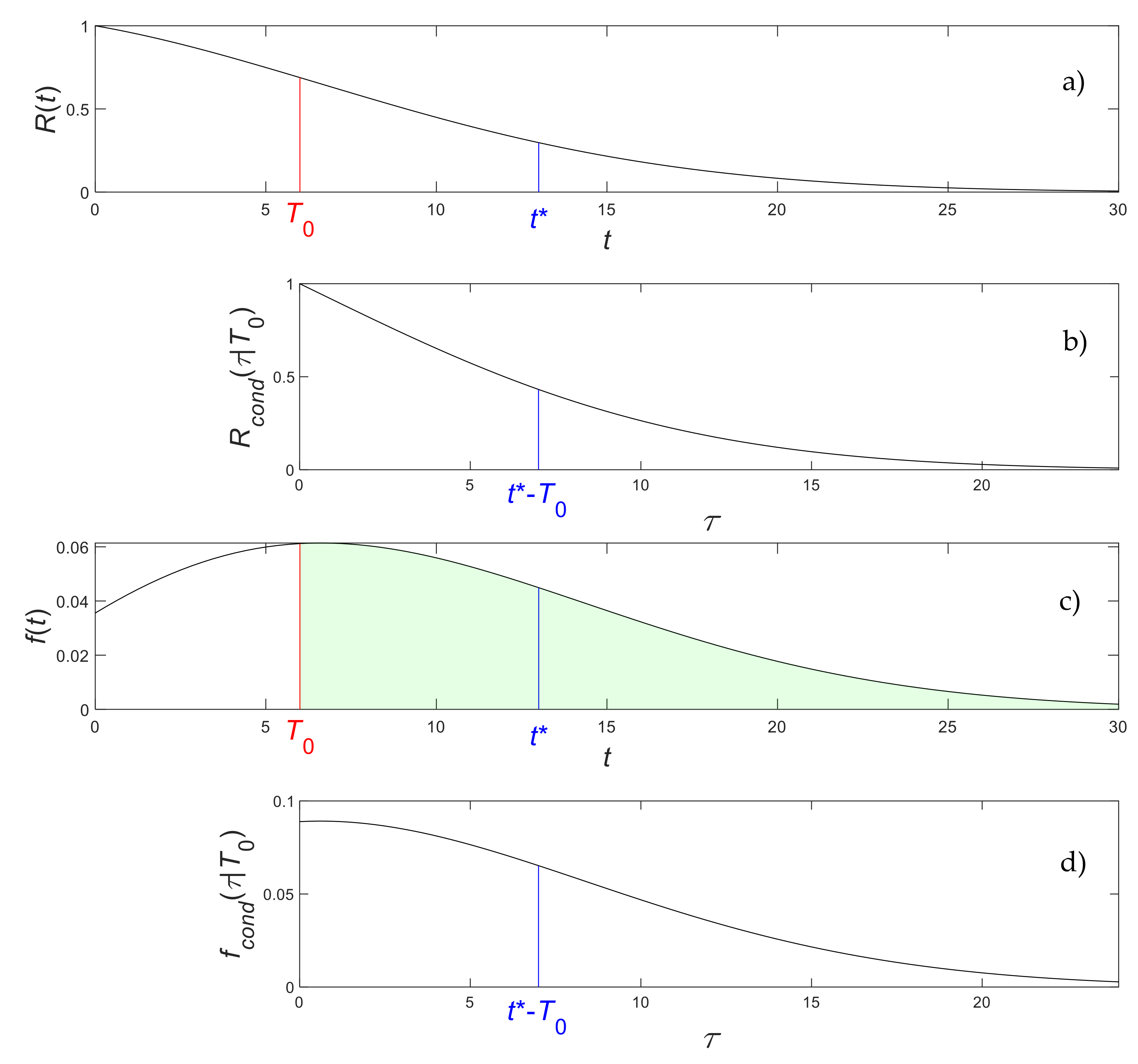
According to Equation (24) the conditional truncated distributions coincide with the conditional original distributions. In case t and t_age are known entities we can generate random time-period variates as special cases of the Practical Indirect Sampling Method from Conditional CDF (PISMCF) [17] where the algorithm is motivated, formalized, illustrated, and proven. On its basis we can define a three-attribute procedure, PISMCF(.), which generates numerically stable random time interval variate, $\Delta \tau$, from a given conditional CDF, F(t|T_surv), where T_surv is a non-negative real number representing the time of survival:

$$\Delta \tau =\mathrm{PISMCF}\left(F\left(.\right),F^{-1}\left(.\right),T_{surv}\right)$$

(25)

In Equation (25), F(.) is the unconditional CDF which can express F(t|T_surv) using Equation (26):

$$1-F\left(t|T_{surv}\right)=\frac{1-F\left(t+T_{surv}\right)}{1-F\left(T_{surv}\right)}$$

(26)

The second argument, F^–1(.), of the PISMCF procedure from Equation (25) being the inverse CDF, can be used to estimate the time t_λ where the denominator of Equation (26) is 100 machine epsilons (ϵ):

$$t_{\lambda }=F^{-1}\left(1-100\epsilon \right)$$

(27)

In short, the algorithm for estimating Equation (25) is: (a) Calculate t_λ using Equation (27); (b) if T_surv < t_λ, then set T_cut = T_surv, else set T_cut = t_λ; (c) Generate RD as a uniformly distributed variate in the unit interval (0,1); (d) estimate p_RD = 1 − RD [1 − F(T_cut)]; (e) Set $\Delta \tau =F^{-1}\left(p_{RD}\right)$.

Let us assume that while performing the simulation of the jth pseudo-reality for the 2SBRSBF system we have observed only the first k_cur state events. The simulation probably will continue and therefore, the EC is yet incomplete:

$$E{C}_j^{inc}=\left\{\left[timeps{r}_j\left(k\right),stateps{r}_j\left(k\right)\right]\left|k=1,2\right.,\cdots ,k_{cur}\right\}$$

(28)

Then, the current state of the system is s_cur = statespr_j(k_cur) and the simulational time is T_cur = timespr_j(k_cur) < t_end (see EC property p3). The incomplete EC in Equation (28) is never empty since k_cur ≥ 1 (see EC properties p1, p3, and p5).

If s_cur > 3, we do not need to generate any time-period variates since it shows a system failure, i.e., end of the simulation in the jth pseudo-reality (see EC properties p8, p11, and p6).

If s_cur is 1, we need to generate two possible time-period variates: the time to failure of the primary unit, $\Delta {\tau }_{1,fp}$, and the time to failure in standby of the backup unit, $\Delta {\tau }_{1,fb}$. Using Equation (25):

$$\Delta {\tau }_{1,fp}=\mathrm{PISMCF}\left(F_1\left(.\right),F_1^{-1}\left(.\right),T_{cur}\right)$$

(29)

$$\Delta {\tau }_{1,fb}=\mathrm{PISMCF}\left(F_3\left(.\right),F_3^{-1}\left(.\right),T_{cur}\right)$$

(30)

If s_cur is 3, we do not need to generate any time-period variate since the possible time to failure of the primary unit is known to be $\left(\Delta {\tau }_{1,fp}-\Delta {\tau }_{1,fb}\right)$, where $\Delta {\tau }_{1,fp} \mathrm{and} \Delta {\tau }_{1,fb}$ are generated in the previous State 1 (see EC properties p9 and p13).

If s_cur > 3, we do not need to generate any time-period variate since we have observed a system failure of some type which means that the simulation in the jth pseudo-reality should stop and therefore q_j = k_cur (see EC properties p6, p8, and p11).

If s_cur is 2, we need to generate two possible time-period variates: the time to repair of the primary unit, $\Delta {\tau }_{2,rp}$, and the time to failure in operation of the backup unit, $\Delta {\tau }_{2,fb}$. Using Equation (25):

$$\Delta {\tau }_{2,rp}=\mathrm{PISMCF}\left(F_4\left(.\right),F_4^{-1}\left(.\right),T_{cur}\right)$$

(31)

$$\Delta {\tau }_{2,fb}=\mathrm{PISMCF}\left(F_2\left(.\right),F_2^{-1}\left(.\right),t_{age}\right)$$

(32)

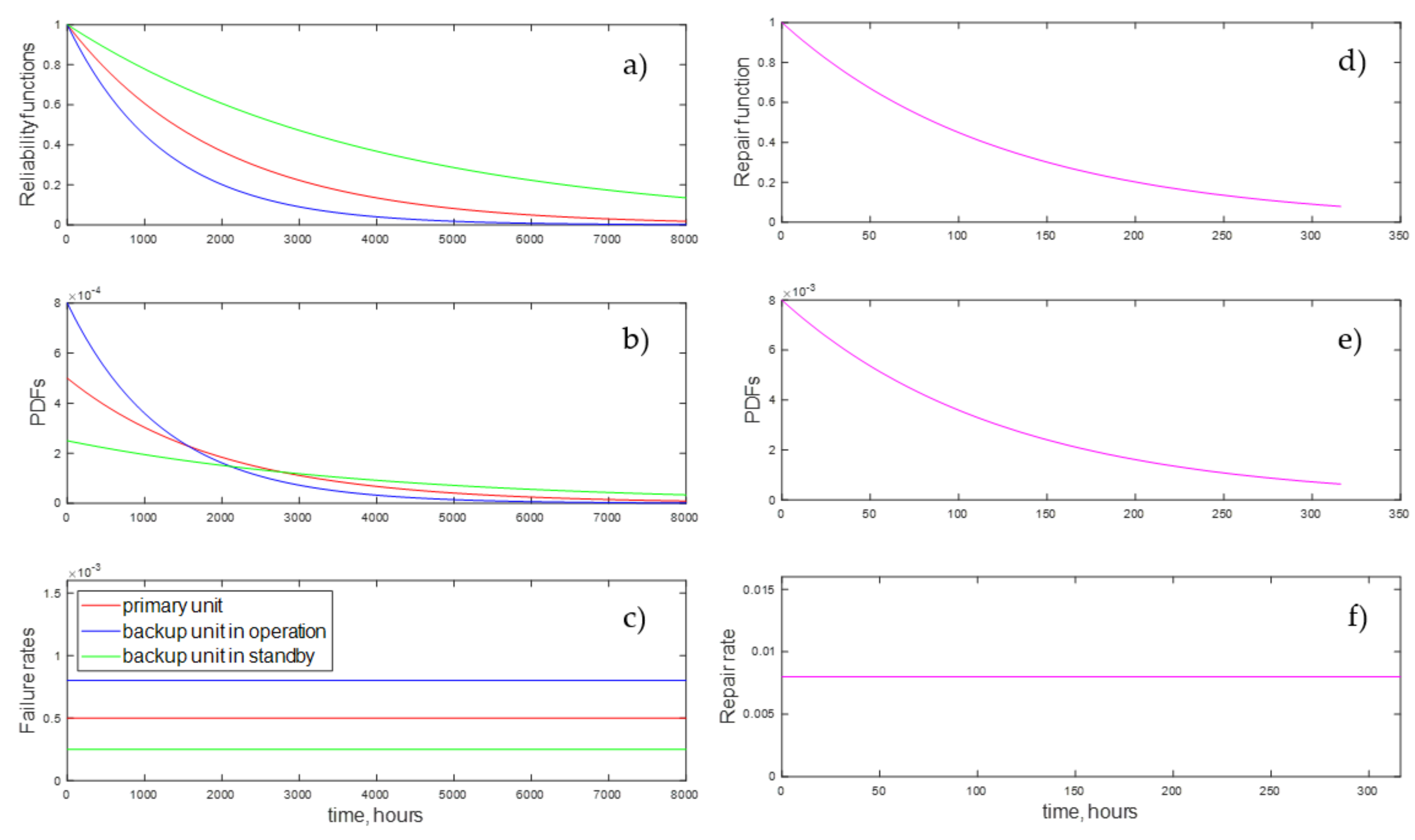
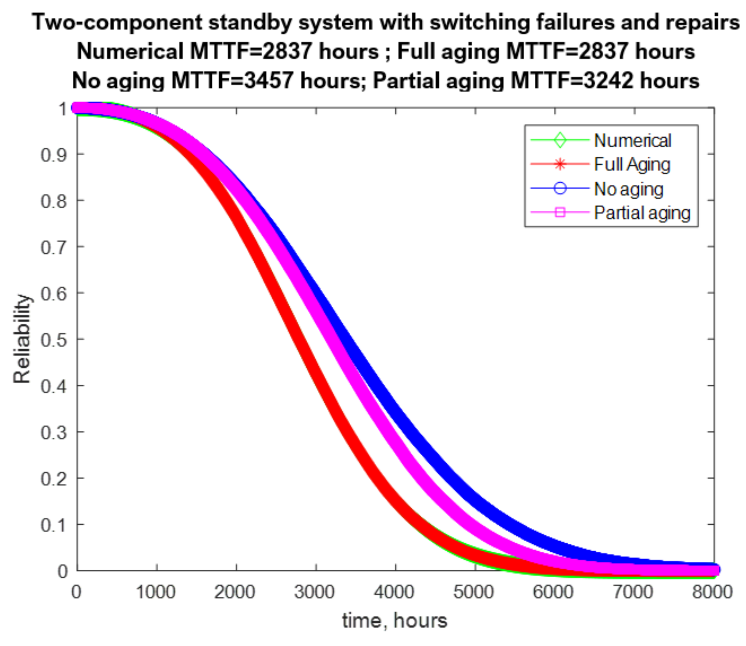
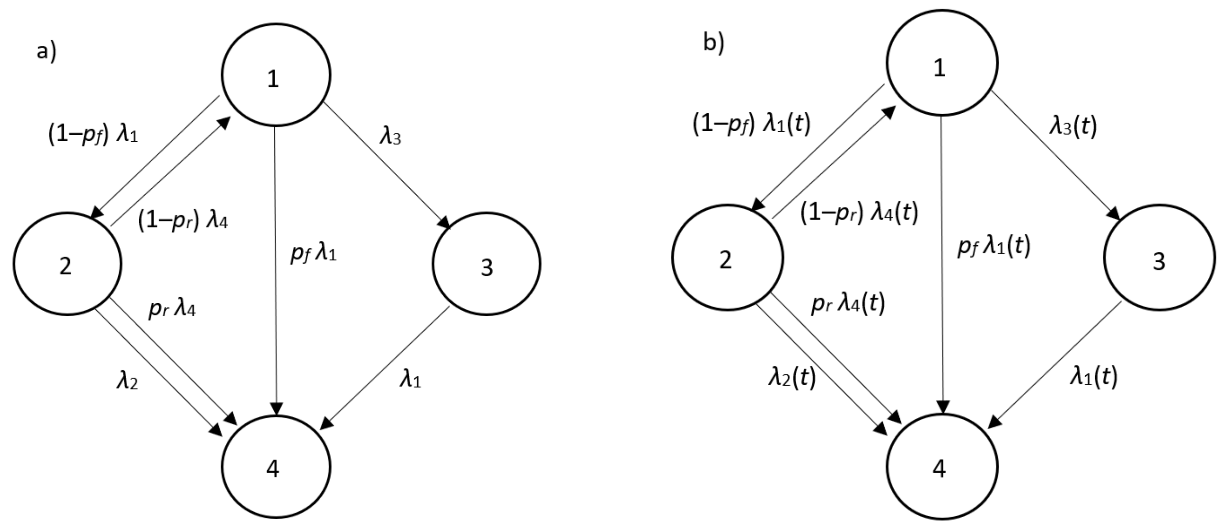
If the 2SBRSBF operates with First Case distributions, the equivalent age, t_age, of the backup unit when it starts operation at time T_cur is rather irrelevant since F₂(.) is the CDF of an exponential distribution. Then we can compare the state probability functions derived by the simulational solution with the same acquired, on one hand, from numerical solution with the DAE system from Equation (16) according to the RD in Figure 1b and on the other hand with the analytical solution from Equations (9)–(12) according to the RD in Figure 1a.

If, however, the 2SBRSBF operates with Second Case distributions, then in order to use Equation (32), we have to determine the equivalent age, t_age, at time T_cur. Since we need $\Delta {\tau }_{2,fb}$ only when the system is State 2, it follows that k_cur is even (see EC property p9). From the beginning of the jth pseudo-reality up to time T_cur, the backup component has been in standby (k_cur/2) times when the primary component was operating till its failure (see EC property p9). Up to T_cur, the backup component has never failed in standby when the primary component was in operation, i.e., during the compound time interval with overall positive length T_sb (see EC properties p6, p8, and p9). The latter time length can be defined using Equation (28) as:

$$T_{sb}={\displaystyle \sum _{i=1}^{k_{cur}/2}\left[timeps{r}_j\left(2i\right)-timeps{r}_j\left(2i-1\right)\right]}$$

(33)

On the other hand, the backup component has been in operation (k_cur/2 − 1) times, when the primary component was in successful repair (see EC property p9). Up to T_cur, the backup component has never failed during operation when the primary component was successfully repaired, i.e., during the compound time interval with overall non-negative length T_oper time (see EC properties p7, p8, and p9). The latter time length can be estimated by noting that up to T_cur the 2SBRSBF system is either in State 1 or in State 2:

$$T_{oper}=T_{cur}-T_{sb}$$

(34)

The non-negative value of t_age will be the sum of the backup component operation time, T_oper, with the equivalent operating time $T_{equ}$ with which the backup component would age during the standby time T_sb:

$$t_{age}=T_{oper}+T_{equ}$$

(35)

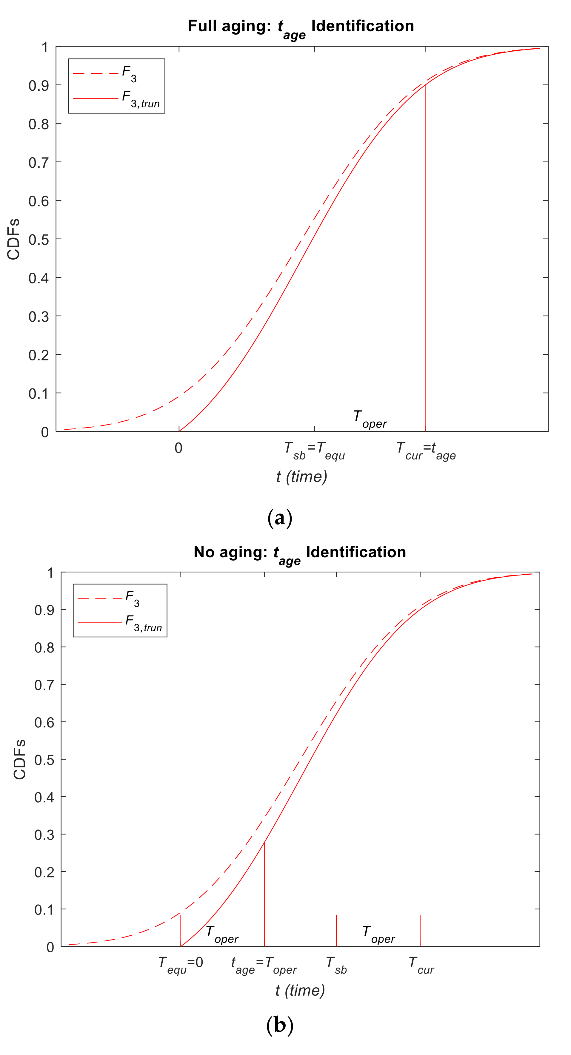
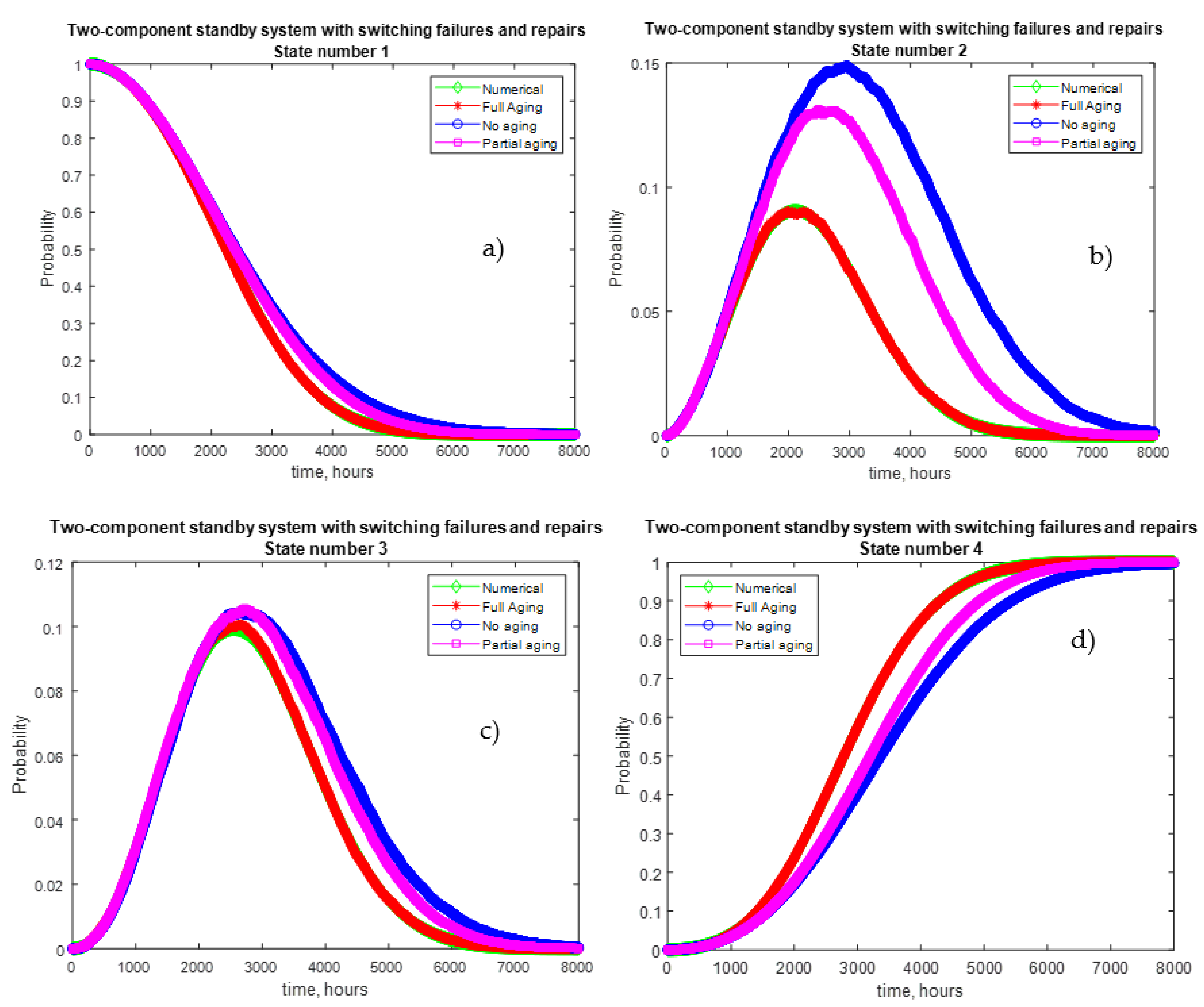
The equivalent operating time $T_{equ}$ depends on aging in standby mechanism under which the 2SBRSBF system functions. There are three alternative assumptions for the nature of this aging in standby mechanism: full aging, no aging, or partial aging.

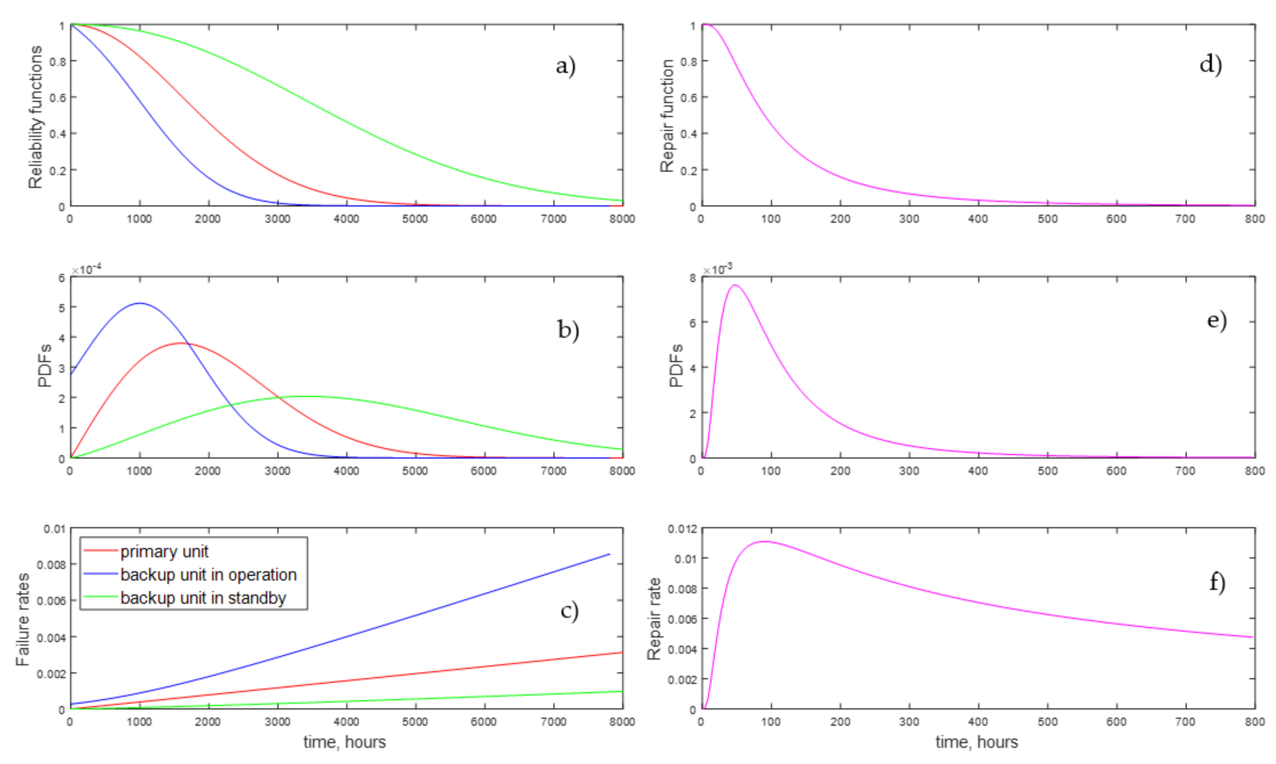
The full aging assumption accepts that the aging of the backup component during standby is the same as during operation (see Figure 2a):

$$T_{equ}=T_{sb}\Rightarrow t_{age}=T_{oper}+T_{sb}=T_{cur}-T_{sb}+T_{sb}=T_{cur}$$

(36)

Under the full aging assumption, a 2SBRSBF can be described with the DAE system from Equation (16) according to the RD in Figure 1b, which allows us to acquire numerical solution for Second Case distributions. The numerical solution can be compared with simulational state probability functions.

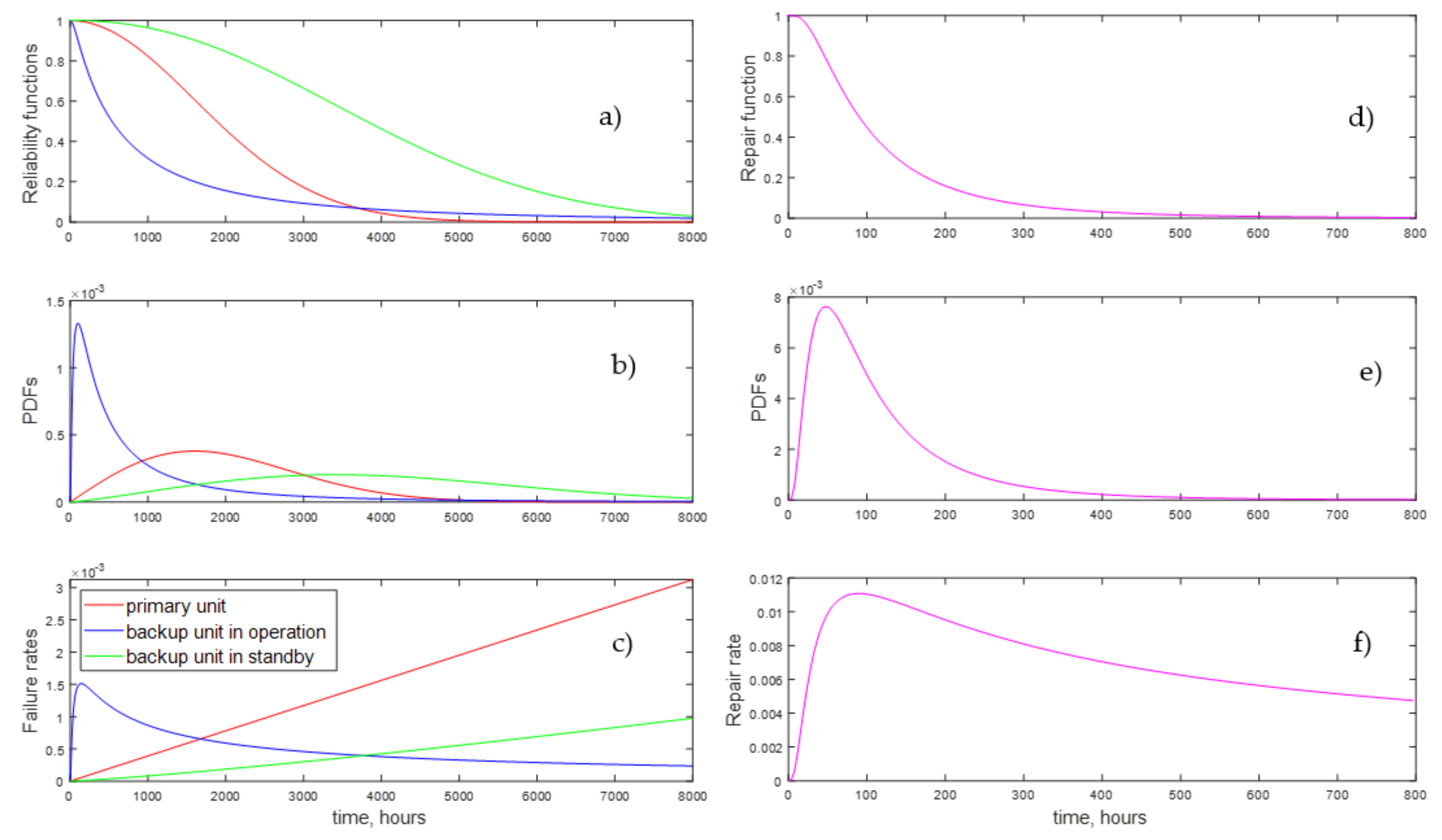
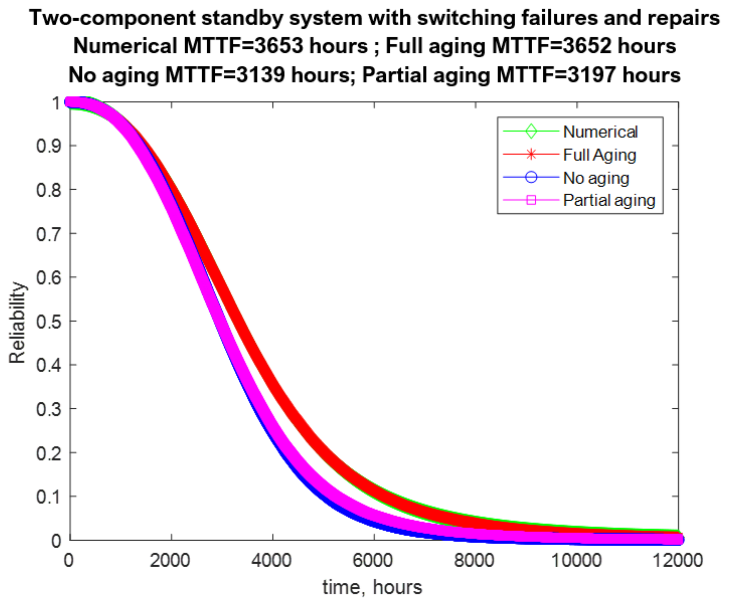
The no aging assumption accepts that the backup component during standby never ages (see Figure 2b):

$$T_{equ}=0\Rightarrow t_{age}=T_{oper}+0=T_{cur}-T_{sb}$$

(37)

Under the no aging assumption, a 2SBRSBF cannot be described with a DAE system since no RD adequately reflects the reliability behavior of the 2SBRSBF. For Second Case distributions, the only possible solution is the simulational one.

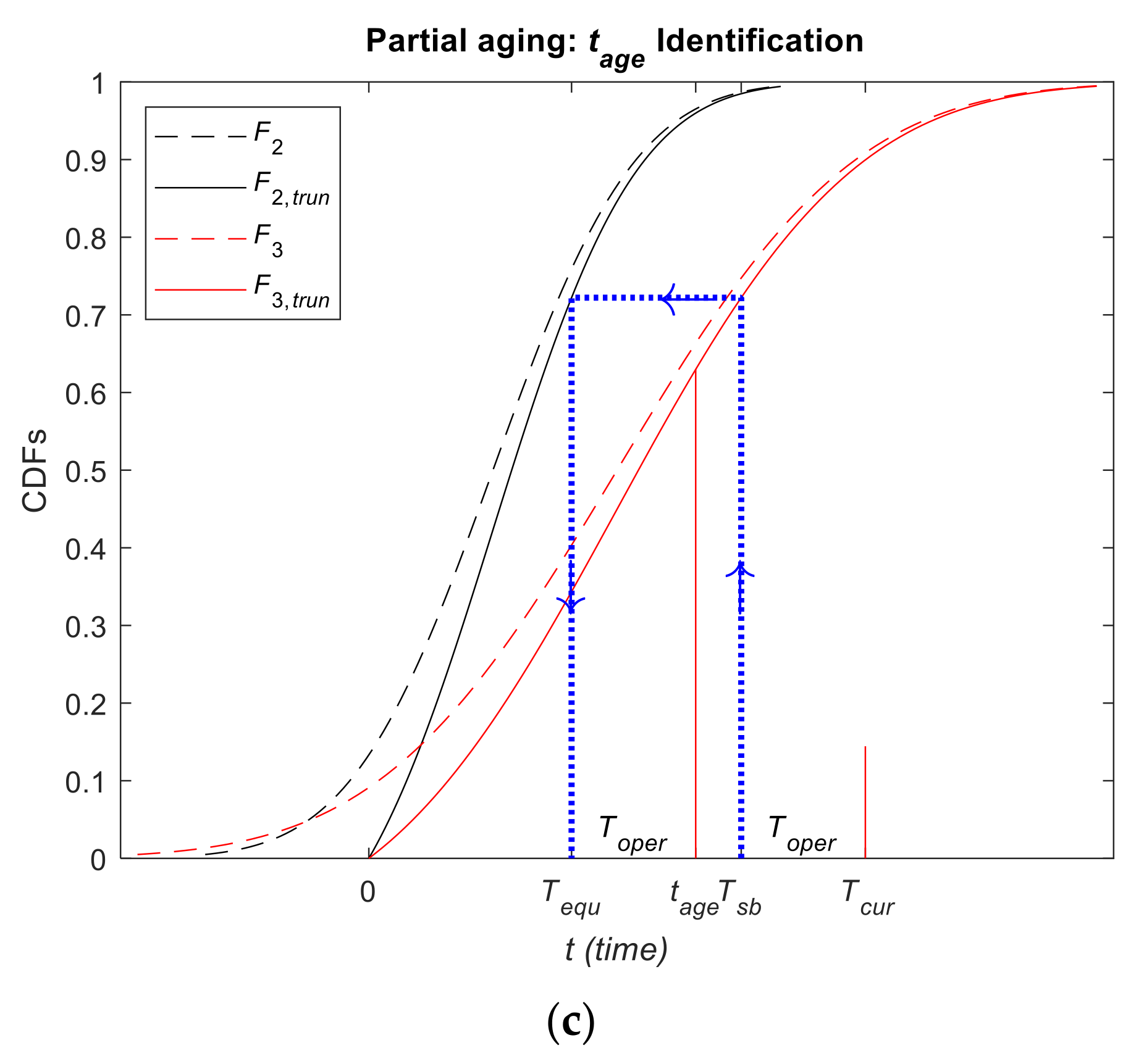
The partial aging assumption accepts that the backup component in standby ages to the same reliability as the backup component in operation during the equivalent operating time $T_{sb}^{equ}$ (see Figure 2c):

$$F_{2,trun}\left(T_{sb}^{equ}\right)=F_{3,trun}\left(T_{sb}\right)$$

(38)

Equation (38) in simplified form was firstly proposed in [22], where it was successfully tested for Two-Component Standby System with Failures in Standby. In a real 2SBRSBF system, the failures of the backup component will be more frequent during operation than during standby which means that F_2,trun(t) ≥ F_3,trun(t) for any non-negative time t. This inequality, together with Equation (38), assures that practically always $T_{equ}\in \left[0,T_{sb}\right]$. Applying Equation (15) twice to Equation (38) we get:

$$T_{equ}=\left\{\begin{array}{cc}{F}_2^{-1}\left(p^{equ}\right)& if p^{equ}<1-100\epsilon \\ t_{\lambda ,2}& if p^{equ}\ge 1-100\epsilon \end{array}\right., \mathrm{where} p^{equ}=1-\frac{1-F_2\left(0\right)}{1-F_3\left(0\right)}\left[1-F_3\left(T_{sb}\right)\right]$$

(39)

In Equation (39), $t_{\lambda ,2}$ is calculated with Equation (13) for k = 2, therefore it uses the ideas in Equation (14) for stable approximation of the equivalent operating time, $T_{equ}$, at any $T_{cur}\in \left[0,t_{end}\right]$ for arbitrary incomplete EC from Equation (23) describing the behavior of a 2SBRSBF.

Under the partial aging assumption, the 2SBRSBF cannot be described with a DAE system since no RD adequately reflects the reliability behavior of the 2SBRSBF similarly to the no aging assumption. Again, for Second Case distributions, the only possible solution is the simulational one.

We combined Equations (33)–(37) into a six-attribute procedure, TAGEASS(.), which gives numerically stable estimates for the equivalent age, t_age, of the backup unit under any of the three aging assumptions:

$$t_{age}=\mathrm{TAGEASS}\left(F_2\left(.\right),F_2^{-1}\left(.\right),F_3\left(.\right),E{C}_j^{inc},T_{cur},Fla{g}_A\right)$$

(40)

In Equation (40), the variable Flag_A is 1, 2 or 3, respectively when the 2SBRSBF operates under the full aging, no aging, or partial aging assumptions. Then Equation (40) can be estimated using Algorithm 1.

Algorithm 1 Equivalent Age Estimation in the jth Pseudo-Reality for 2SBRSBF

1) Calculate the total standby time of the backup component, Tsb, using (33). 2) Calculate the total operational time of the backup component, Toper, using (34). 3) If FlagA = 1 (full aging assumption), then calculate the equivalent operating time, Tequ, using (36). 4) If FlagA = 2 (no aging assumption), then calculate the equivalent operating time, Tequ, using (37). 5) If FlagA = 3 (partial aging assumption), then: 5.1) Calculate the positive constant, $t_{\lambda ,2}$, using (13) with k = 2. 5.2) Calculate the probability, pequ, using the second part of (39). 5.3) Calculate the equivalent operating time, Tequ, the first part of (39) 6) Calculate the equivalent age of the backup component, tage, using (35).

6.3. Event Chain Generation for 2SBRSBF

After developing the procedures for random time-period generation in Section 6.2, we may simulate an EC for the jth pseudo-reality of a 2SBRSBF system which satisfies all EC properties defined in Section 6.1.

The following is given:

(1)

For each k = 1, 2, 3, 4, the original CDFs, F_k(t), defined for any real argument.

(2)

For each k = 1, 2, 3, 4 the original inverse CDFs $F_k^{-1}\left(p\right)$, defined for any p belonging to the unit interval.

(3)

The probability, p_f, for switching failure on demand.

(4)

The probability, p_r, for back-switching failure on demand.

(5)

The value of the Flag_A, which determines under which aging assumption the 2SBRSBF operates.

(6)

The positive final simulation time, t_end, such that $R_{sys}\left(t_{end}\right)\approx 0 (<0.01)$.

(7)

The consecutive number, j, of the pseudo-reality.

The event chain for the jth pseudo-reality, EC_j can be calculated using Algorithm 2.

Algorithm 2 Generation of the Event Chain for the jth Pseudo-Reality of 2SBRSBF

1)  Initiate the incomplete event chain, $E{C}_j^{inc}$: 1.1) Set, Tcur =0 (the current system time is zero) 1.2) Set, kcur = 1 (the current count of events is one) 1.3) Set, timepsrj(kcur) = Tcur (the time of the first event is zero) 1.4) Set, statepsrj(kcur) = 1 (the system starts from State 1) 2)  If statepsrj(kcur) = 1 (the system is currently in State 1), then: 2.1) Estimate, $\Delta {\tau }_{1,fp}=\mathrm{PISMCF}\left(F_1\left(.\right),F_1^{-1}\left(.\right),T_{cur}\right)$ (the possible time to failure of the primary unit). 2.2) Estimate, $\Delta {\tau }_{1,fb}=\mathrm{PISMCF}\left(F_3\left(.\right),F_3^{-1}\left(.\right),T_{cur}\right)$ (the possible time to standby failure of the backup unit). 2.3) If $t_{end}\le T_{cur}+\Delta {\tau }_{1,fp}$ and $t_{end}\le T_{cur}+\Delta {\tau }_{1,fb}$ (the end of simulation comes first), then: 2.3.1) Set qj = kcur (the last event count in ECj) 2.3.2) Set $E{C}_j=E{C}_j^{inc}$ (the final ECj) 2.3.3) Stop the Algorithm 2.4) If $\Delta {\tau }_{1,fp}\le \Delta {\tau }_{1,fb}$ (the primary unit is failing first), then: 2.4.1) Set kcur= kcur +1 (new event) 2.4.2) Set Tcur= Tcur + $\Delta {\tau }_{2,fb}$ (new current system time) 2.4.3) Set timepsrj(kcur) = Tcur (the time of the new event) 2.4.4) Generate RN as an evenly distributed number in the unit interval (check which is the new state) 2.4.4.1) If RN > pf, then statepsrj(kcur) = 2 (i.e., no switching failure, move to State 2) 2.4.4.1) If RN ≤ pf, then statepsrj(kcur) = 41 (i.e., switching failure, move to State 4, type a) 2.5) If $\Delta {\tau }_{1,fp}>\Delta {\tau }_{1,fb}$ (the backup unit is failing first), then: 2.5.1) Set kcur= kcur + 1 (new event) 2.5.2) Set Tcur= Tcur + $\Delta {\tau }_{1,fb}$ (new current system time) 2.5.3) Set timepsrj(kcur) = Tcur (the time of the new event) 2.5.4) Set statepsrj(kcur) = 3 (move to State 2) 3)  If statepsrj(kcur) = 2 (the system is currently in State 2), then: 3.1) Estimate, $\Delta {\tau }_{2,rp}=\mathrm{PISMCF}\left(F_4\left(.\right),F_4^{-1}\left(.\right),T_{cur}\right)$ (the possible time to repair of the primary unit). 3.2) Estimate $t_{age}=\mathrm{TAGEASS}\left(F_2\left(.\right),F_2^{-1}\left(.\right),F_3\left(.\right),E{C}_j^{inc},T_{cur},Fla{g}_A\right)$ (the equivalent age of the backup unit) 3.3) Estimate, $\Delta {\tau }_{2,fb}=\mathrm{PISMCF}\left(F_2\left(.\right),F_2^{-1}\left(.\right),t_{age}\right)$ (the possible time to operational failure of the backup unit). 3.4) If $t_{end}\le T_{cur}+\Delta {\tau }_{2,rp}$ and $t_{end}\le T_{cur}+\Delta {\tau }_{2,fb}$ (the end of simulation comes first), then: 3.4.1) Set qj = kcur (the last event count in ECj) 3.4.2) Set $E{C}_j=E{C}_j^{inc}$ (the final ECj) 3.4.3.) Stop the Algorithm 3.5) If $\Delta {\tau }_{2,rp}\le \Delta {\tau }_{2,fb}$ (the primary unit is repaired first), then: 3.5.1) Set kcur = kcur + 1 (new event) 3.5.2) Set Tcur = Tcur + $\Delta {\tau }_{2,rp}$ (new current system time) 3.5.3) Set, timepsrj(kcur) = Tcur (the time of the new event) 3.5.4) Generate RN as an evenly distributed number in the unit interval (check which is the new state) 3.5.4.1) If RN > pr, then statepsrj(kcur) =1 (no back-switching failure, move to State 1) 3.5.4.2) If RN ≤ pr, then statepsrj(kcur) = 40 (back-switching failure, move to State 4, type b) 3.6) If $\Delta {\tau }_{2,rp}>\Delta {\tau }_{2,fb}$ (the backup unit is failing first), then: 3.6.1) Set, kcur = kcur + 1 (new event) 3.6.2) Set, Tcur = Tcur + $\Delta {\tau }_{2,fb}$ (new current system time) 3.6.3) Set, timepsrj(kcur) = Tcur (the time of the new event) 3.6.4) Set, statepsrj(kcur) =42 (move to State 4, type c) 4)  If statepsrj(kcur) = 3 (the system is currently in State 3), then: 4.1) If $t_{end}\le T_{cur}+\Delta {\tau }_{1,fp}-\Delta {\tau }_{1,fb}$ (the end of simulation comes first), then: 4.1.1) Set, qj= kcur (the last event count in ECj) 4.1.2) Set, $E{C}_j=E{C}_j^{inc}$ (the final ECj) 4.1.3) Stop the Algorithm 4.2) If $t_{end}>T_{cur}+\Delta {\tau }_{1,fp}-\Delta {\tau }_{1,fb}$ (the primary unit is failing first), then: 4.2.1) Set, kcur= kcur+1 (new event) 4.2.2) Set, Tcur= Tcur+$\Delta {\tau }_{1,fp}-\Delta {\tau }_{1,fb}$ (new current system time) 4.2.3) Set, timepsrj(kcur) = Tcur (the time of the new event) 4.2.4) Set, statepsrj(kcur) = 43 (switching failure, move to State 4, type d) 5)  If statepsrj(kcur) > 3 (the system is currently in State 4), then: 5.1) Set, qj = kcur (the last event count in ECj) 5.2) Set, $E{C}_j=E{C}_j^{inc}$ (the final ECj) 5.3) Stop the Algorithm 6)  Go to Step 2 (try a next transition)

It is easy to demonstrate that any EC generated by Algorithm 2 satisfies all EC properties formulated in Section 6.1.

6.4. Extracting Reliability Information from the Simulated ECs

Let N be a large positive integer representing the count of the randomly simulated pseudo-realities. Using Algorithm 2, we can simulate EC_j, for j = 1,2, …, N. In this section, we will extract the reliability information from the simulated ECs, approach which is the essence of any Monte Carlo simulation [37] (pp. 290–294).

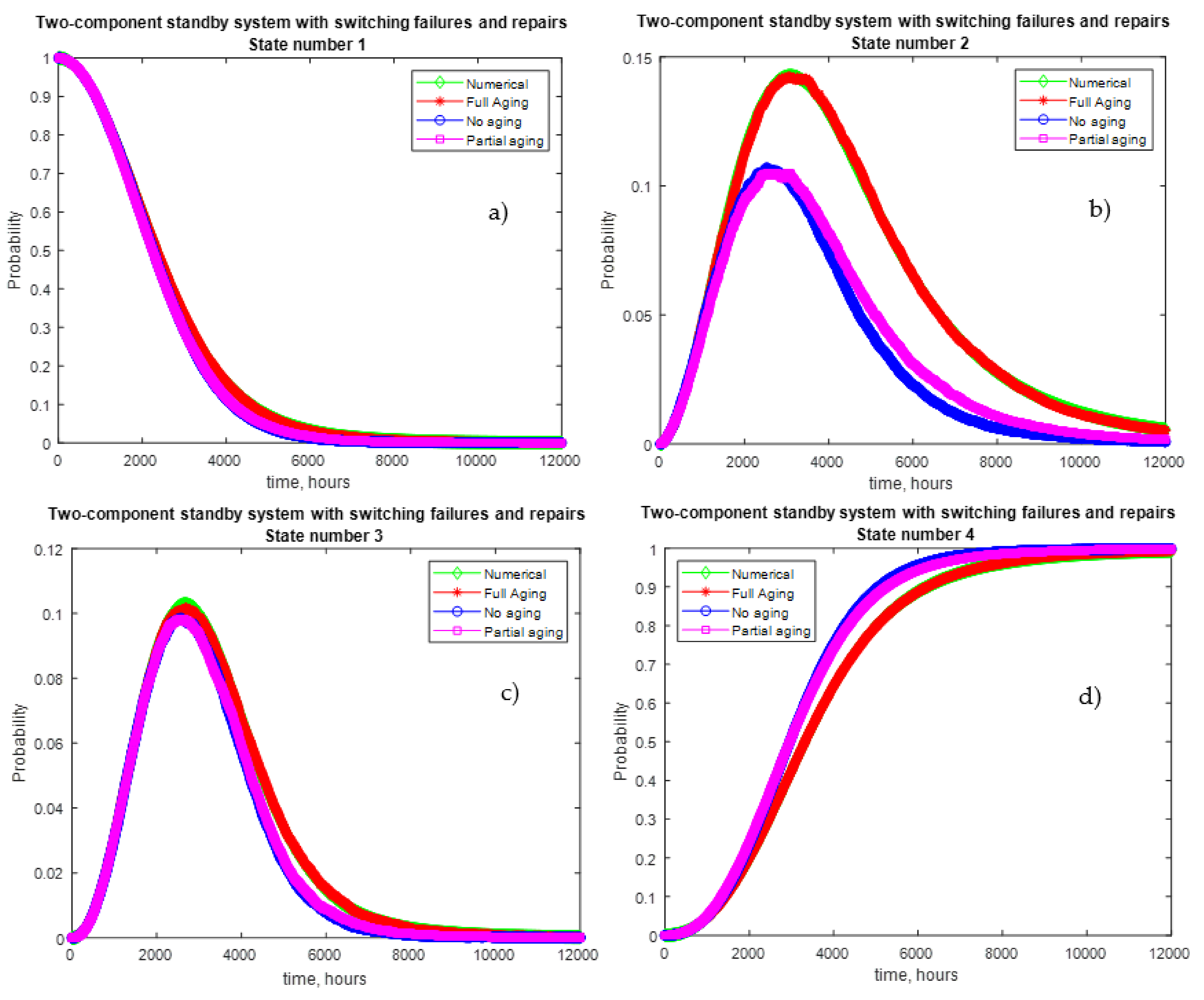
Let us calculate the state probability functions at the 2000 evenly distributed time points from 0 to t_end given in Equation (20). For a given EC_j we can estimate the state, St_i,j, at each of the time points t_i:

$$S{t}_{i,j}=\left\{\begin{array}{l}stateps{r}_j\left(k\right)\hspace{1em}\hspace{1em}\mathrm{if} timeps{r}_j\left(k\right)\le t_i<timeps{r}_j\left(k+1\right)\hspace{1em}\hspace{1em},\mathrm{for} k<q_j\hfill \\ stateps{r}_j\left(q_j\right)\hspace{1em}\hspace{1em}\mathrm{if} timeps{r}_j\left(q_j\right)\le t_i\le t_{end}\hfill \end{array}\right., \mathrm{where} \begin{array}{c}i=1,2,\dots ,2000\\ j=1,2,\dots ,N\end{array}$$

(41)

From Equation (41) it is easy to estimate the values of the first three state probability functions at the time point, t_i:

$$P_g\left(t_i\right)=\frac{1}{N}\#\left(S_{i,j}=g|j=1,2,\dots ,N\right), \mathrm{where} g=1,2,3 \mathrm{and} i=1,2,\dots ,2000$$

(42)

In Equation (42) the $\#\left(S_{i,j}=g|j=1,2,\dots ,N\right)$ is the count of all states at the time point t_i which are equal to g.

The fourth state probability function can be estimated using Equation (1) as:

$$P_4\left(t_i\right)=1-P_3\left(t_i\right)-P_2\left(t_i\right)-P_3\left(t_i\right) , \mathrm{for} i=1,2,\dots ,2000$$

(43)

The reliability function and the MTTF_sys can be approximated with Equations (21) and (22). According to the ES property p1, the reliability in Equation (22) has decreasing nodes:

$$R_{sys}\left(t_i\right)\ge R_{sys}\left(t_{i+1}\right) , \mathrm{for} i=1,2,\dots ,1999$$

(44)

One way to identify the α-design life, t_des,α for given α is to transform the nodes, $\left\{\left[t_i,R_{sys}\left(t_i\right)\right]|i=1,2,\dots ,2000\right\}$, of the system reliability from Equation (22) into strictly decreasing purged nodes $\left\{\left[t_i^{pu},R_{sys}^{pu}\left(t_i^{pu}\right)\right]|i=1,2,\dots ,n^{pu}\right\}$ where:

$$R_{sys}^{pu}\left(t_i^{pu}\right)>R_{sys}^{pu}\left(t_i^{pu}\right) , \mathrm{for} i=1,2,\dots ,n^{pu}$$

(45)

Such a purging procedure is proposed in [17], where the algorithm is motivated, formalized, illustrated, and proven. In short, it runs in the steps summarized in Algorithm 3.

Algorithm 3 Purging Algorithm

(a) Identify the time of the first purged node $\left[t_1^{pu},R_{sys}^{pu}\left(t_1^{pu}\right)=1\right]$ as the greatest ti for which $R_{sys}\left(t_i\right)=1$; (b) Substitute all internal nodes with equal reliability with one purged node in the center of the horizontal platform; (c) Identify the time of the last purged node $\left[t_{n^{pu}}^{pu},R_{sys}^{pu}\left(t_{n^{pu}}^{pu}\right)\right]$ as the smallest ti for which $R_{sys}\left(t_i\right)=R_{sys}\left(t_{2000}\right)$.

Having the strictly decreasing purged system reliability function, we can identify the α-design life, t_des,α for any $\alpha \in \left[R_{sys}^{pu}\left(t_{n^{pu}}^{pu}\right),1\right]$:

$$t_{des,\alpha }=t_i^{pu}+\left[R_{sys}^{pu}\left(t_i^{pu}\right)-\alpha \right]\frac{t_{i+1}^{pu}-t_i^{pu}}{R_{sys}^{pu}\left(t_i^{pu}\right)-R_{sys}^{pu}\left(t_{i+1}^{pu}\right)}, \mathrm{for} R_{sys}^{pu}\left(t_i^{pu}\right)\ge \alpha >R_{sys}^{pu}\left(t_{i+1}^{pu}\right)$$

(46)

As discussed in Section 3, the reliability numerical characteristics Median_sys, B1_life, B10_life, and IQR_sys can be estimated as $t_{des,0.5}, t_{des,0.99}, t_{des,0.9}, \mathrm{and} t_{des,0.25}-t_{des,0.75}$ respectively by applying Equation (46) five times.

The simulational solution is universal and exists even when the numerical and analytical solutions are impossible. Even when the numerical and the analytical solutions exist, the simulational solution can provide richer reliability information.

For example, it is obvious that the 2SBRSBF system will have 100% chance to ever be in the State 1. It is also clear that if tend is correctly selected, then the 2SBRSBF system will have more than 99% chance to ever be in the State 4. However, it is interesting to know the chance, P_2,ever, for the 2SBRSBF system to ever be in the State 2, since that probability will help us plan the resources needed for the repair of the primary unit. Similarly, the chance, P_3,ever, for the 2SBRSBF system to ever be in the State 3 is important, since that will show us the prevalence of the failure in standby of the backup unit. So, for a given 2SBRSBF system, we can estimate the chances, P_g,ever, for g = 1,2,3:

$$P_{g,ever}=\frac{100}{N}\#\left(\exists i, \mathrm{that} S_{i,j}=g|j=1,2,\dots ,N\right), \mathrm{where} g=1,2,3$$

(47)

In Equation (47), $\#\left(\exists i, \mathrm{that} S_{i,j}=g|j=1,2,\dots ,N\right)$ is the count of pseudo-realities in which State g can be found at least once. Similarly, for a given 2SBRSBF system we can estimate the chance, P_4,ever as:

$$P_{4,ever}=\frac{100}{N}\#\left(\exists i, \mathrm{that} S_{i,j}>3|j=1,2,\dots ,N\right)$$

(48)

In Equation (48), $\#\left(\exists i, \mathrm{that} S_{i,j}>3|j=1,2,\dots ,N\right)$ is the count of pseudo-realities in which State 4 (system failure) can be found at least once.

As another example for reliability information, which can be acquired neither with the numerical, nor with the analytical solution, can be found in the four conditional chances, $P_{g,ever}^{cond}$ (for g = 40, 41, 42, 43), of the 2SBRSBF system to have respectively type b, type a, type c, or type d system failure, provided that system has failed:

$$P_{g,ever}^{cond}=100\frac{\#\left(S_{i,q_j}=g|j=1,2,\dots ,N\right)}{N{P}_{4,ever}/100}, \mathrm{where} g=40,41,42,43$$

(49)

The information in Equation (49) allows to identify the types of system failures which dominate the 2SBRSBF system. That knowledge will increase the efficiency of the reliability improvement measures. Equations (42), (47)–(49) use the frequentist interpretation of probability [40] (pp. 42–43).

Knowing how to simulate an EC for the jth pseudo-reality of a 2SBRSBF system, allows us to develop the simulational solution of a given 2SBRSBF system. We have the following given:

(1)

For each k = 1, 2, 3, 4, the original CDFs, F_k(t), defined for any real argument.

(2)

For each k = 1, 2, 3, 4, the original inverse CDFs $F_k^{-1}\left(p\right)$, defined for any p belonging to the unit interval.

(3)

The probability, p_f, for switching failure on demand.

(4)

The probability, p_r, for back-switching failure on demand.

(5)

The value of the Flag_A, which determines under which aging assumption the 2SBRSBF operates.

The proposed algorithm in [17] uses simulation to find the reliability characteristics of a two-component standby systems with switching failures and aging in standby. The simulational solution for 2SBRSBF system can be obtained through a generalization of that algorithm, which is formalized as Algorithm 4 below.

Algorithm 4 Simulational Solution of a 2SBRSBF System

1) Select the count N of pseudo-realities to be simulated as a large integer. 2) Select the final simulation time, tend, as a positive real number. 3) Set, j = 1 (initiate the consecutive number of the simulated pseudo-reality) 4) Generate the ECj, using Algorithm 2. 5) Set, j = j + 1 (move to next pseudo-reality). 6) If j ≤ N, then go to Step 4 (repeat the EC generation N times). 7) Estimate 2000 equally spaced times, ti, in the closed interval [0, tend] using Equation (20). 8) Estimate the states, Sti,j, using Equation (41). 9) Estimate the first three state probability functions,$P_g\left(t_i\right) \left(\mathrm{for} g=1,2,3\right)$ at the time points ti using Equation (42). 10) Estimate the fourth state probability function, $P_4\left(t_i\right)$, at the time point ti using Equation (43). 11) Estimate the system reliability function, $R_{sys}\left(t_i\right)$ at the time point ti using Equation (21). 12) Estimate the system mean time to failure,${MTTF}_{sys}$ using Equation (22). 13) Estimate the nodes, $\left\{\left[t_i^{pu},R_{sys}^{pu}\left(t_i^{pu}\right)\right]|i=1,2,\dots ,n^{pu}\right\}$, of the invertible reliability function using Algorithm 3. 14) Estimate the design lives, $t_{des,0.5}, t_{des,0.99}, t_{des,0.9}, t_{des,0.25} \mathrm{and} t_{des,0.75}$ using Equation (46) five times. 15) Set the median time, ${Median}_{sys} = t_{des,0.5}$. 16) Set the B1 life, $t_{des,0.99}$. 17) Set the B10 life, $t_{des,0.9}$. 18) Set the interquartile range, $IQR= t_{des,0.25}- t_{des,0.75}$. 19) Estimate the first three unconditional chances, $P_{g,ever} (\mathrm{for} g= 1,2,3)$ using Equation (47). 20) Estimate the fourth unconditional chance, P4,ever using Equation (48). 21) Estimate the conditional chances, $P_{g,ever}^{cond}$ (for g = 40, 41, 42, 43) using Equation (49).

With the formulation of Algorithm 4 the universal simulational solution for a 2SBRSBF system is complete.

7. Illustrative Examples

7.1. Examples Setup

We shall analyze three Illustrative Examples. In all of them, the probability for switching failure is p_f = 0.12, whereas the probability for back-switching failure is p_r = 0.03. The ratio between those values is plausible for the following reasons. If the switching is successful, it means that the switching device operated properly. Then a back-switching failure is less probable since it will be demanded shortly afterwards (the repair time of the primary component is much smaller than its failure time).

In Example 1, any of the four original distributions has a constant failure/repair rate λ_k shown in

Table 2. Description of the original distributions in Example 1.

Component—Event—Mode	Distribution	Parameters
Primary Component Failure	Exponential	λ1 = 0.0005 failures/h
Backup Component Failure in operation	Exponential	λ2 = 0.0008 failures/h
Backup Component Failure in standby	Exponential	λ3 = 0.00025 failures/h
Primary Component Repair	Exponential	λ4 = 0.008 failures/h

(for k = 1,2,3,4). The PDFs of the original exponential distributions are:

$$f_k\left(t\right)={\lambda }_k{e}^{-{\lambda }_{k}t}, \mathrm{for} t\ge 0 \mathrm{where} k=1,2,3,4$$

(50)

The PDFs, the reliability/repair functions, and the failure/repair rates of the truncated distributions from Equation (50) are plotted in Figure 3. Example 1 will illustrate the behavior of the 2SBRSBF system with First Case distributions. Here, the original and the truncated distributions coincide.

In Example 2, the original distributions are as follows:

(1)

a Rayleigh distribution with shape parameter b₁ [41] for the failures of the primary component:

$$f_1\left(t\right)=\left(t/b_1\right)e^{-0.5{\left(t/b_1\right)}^2}, \mathrm{for} t\ge 0$$

(51)

(2)

a normal distribution with mean value μ₂ h and standard deviation σ₂ h [42] for the failures of the backup component in operation:

$$f_2\left(t\right)=\frac{1}{\sqrt{2\pi }{\sigma }_2}{e}^{-0.5{\left(t-{\mu }_2\right)}^2/{\left({\sigma }_2\right)}^2}, \mathrm{for} t\in \left(-\infty ,+\infty \right)$$

(52)

(3)

a Weibull distribution with a scale parameter θ₃ h and a shape parameter β₃ [43] for the failures of the backup component in standby:

$$f_3\left(t\right)=\frac{{\beta }_3}{{\theta }_3}{\left(\frac{t}{{\theta }_3}\right)}^{{\beta }_3-1}{e}^{-{\left(t/{\theta }_3\right)}^{{\beta }_3}}, \mathrm{for} t\ge 0$$

(53)

(4)

a lognormal distribution with median time t_med,4 h and shape parameter s₄ [44] for the repairs of the primary component:

$$f_4\left(t\right)=\frac{1}{\sqrt{2\pi }{s}_{4}t}{e}^{-0.5{\ln }^2\left(t/t_{med,4}\right)/{\left(s_4\right)}^2}, \mathrm{for} t\ge 0$$

(54)

The original distribution Example 2 are described in

Table 3. Description of the original distributions in Example 2.

Component—Event—Mode	Distribution	Parameters
Primary Component Failure	Rayleigh	b1 = 1600 h
Backup Component Failure in operation	normal	μ2 = 1000 h and σ2 = 900 h
Backup Component Failure in standby	Weibull	θ3 = 4500 h and β3 = 2.2
Primary Component Repair	lognormal	tmed,4 = 90 h and s4 = 0.8

. The PDFs, the reliability/repair functions, and the failure/repair rates of the truncated distributions from Equations (51)–(54) are plotted in Figure 4. Example 2 will illustrate the behavior of the 2SBRSBF system with Second Case distributions where the failures of the backup component in operation have an Increasing Failure Rate (IFR). Such a typical situation can occur when the operational failure is caused mainly by high wearing in the backup component [11] (pp. 73–75). Here, the original and the truncated distributions coincide except for the f₂(t) and f_2,trunc(t).

In Example 3 the distributions are the same as in Example 2, except for the second type, which changes to:

2) a lognormal distribution with median time t_med,2 h and shape parameter s₂ for the failures of the backup component in operation:

$$f_2\left(t\right)=\frac{1}{\sqrt{2\pi }{s}_{2}t}{e}^{-0.5{\ln }^2\left(t/t_{med,2}\right)/{\left(s_2\right)}^2}, \mathrm{for} t\ge 0$$

(55)

The original distribution Example 3 are described in

Table 4. Description of the original distributions in Example 3.

Component—Event—Mode	Distribution	Parameters
Primary Component Failure	Rayleigh	b1 = 1600 h
Backup Component Failure in operation	lognormal	tmed,2 = 537 h and s2 = 1.3
Backup Component Failure in standby	Weibull	θ3 = 4500 h and β3 = 2.2
Primary Component Repair	lognormal	tmed,4 = 90 h and s4 = 0.8

. The PDFs, the reliability/repair functions, and the failure/repair rates of the truncated distributions from Equations (51), (53)–(55) are plotted in Figure 5. Example 3 will illustrate the behavior of the 2SBRSBF system with Second Case distributions where the failures of the backup component in operation have a Decreasing Failure Rate (DFR). Such an atypical situation can occur when the operational failure is caused mainly by high child mortality in the backup component [11] (pp. 73–75). Here, the original and the truncated distributions coincide.

7.2. Example 1 Solution

Since in Example 1, we are dealing with First Case distributions, the type of aging has no effect on the reliability performance of the 2SBRSBF system. The simulation solution was obtained by Algorithm 4 with N = 10,000 pseudo-realities for time from 0 to t_end = 20,000 h. Four typical pseudo-realities are shown in

Table 5. Four typical pseudo-realities from Example 1.

1	Time 0.0 h: Start of the simulation. The primary component operates, the backup component is ready.	Time 0.0 h: Start of the simulation. The primary component operates, the backup component is ready.	Time 0.0 h: Start of the simulation. The primary component operates, the backup component is ready.	Time 0.0 h: Start of the simulation. The primary component operates, the backup component is ready.
2	Time 1378.3 h: The primary component fails in operation. The primary component under repair, the backup component operates.	Time 1753.2 h: The primary component fails in operation. The primary component under repair, the backup component operates.	Time 2016.9 h: The primary component fails in operation. The primary component under repair, the backup component operates.	Time 2348.6 h: The primary component fails in operation. The primary component under repair, the backup component operates.
3	Time 1467.6 h: The primary component successfully repaired. The primary component operates, the backup component is ready.	Time 1821.4 h: The primary component successfully repaired. The primary component operates, the backup component is ready.	Time 2042.9 h: The primary component successfully repaired. The primary component operates, the backup component is ready.	Time 2406.5 h: The primary component successfully repaired. The primary component operates, the backup component is ready.
4	Time 2099.6 h: The primary component fails in operation. Switching failure. Type a system failure (switching failure).	Time 4321.5 h: The primary component fails in operation. The primary component under repair, the backup component operates.	Time 8168.7 h: The primary component fails in operation. The primary component under repair, the backup component operates.	Time 3057.8 h: The backup component fails in standby. The primary component operates, the backup component failed in standby.
5		Time 4460.6 h: The primary component successfully repaired. Back-Switching failure. Type b system failure (back-switching failure).	Time 8288.8 h: The backup component fails in operation. Type c system failure (backup component failure during primary repair).	Time 3712.4 h: The primary component fails in operation. Type d system failure (standby failure+ primary failure).

where the different types of system failures are demonstrated. The four state probability functions are shown in Figure 6a–d, respectively. The system reliability function is depicted in Figure 7. The simulation reliability at t_end was negligible (as required R_sys(20,000) = 0.0024 < 0.01) which justifies the selection of t_end. Important simulation numerical characteristics of the 2SBRSBF reliability can be found in

Table 6. Reliability characteristics of the 2SBRSBF from Example 1.

Count of pseudo-realities	100,000
Simulation time	2.000 × 10+4 h
Mean value (Simulation)	4.294 × 10+3 h
Median	3.418 × 10+3 h
Interquartile range	4.187 × 10+3 h
B10 life	7.922 × 10+2 h
B1 life	1.174 × 10+2 h
Mean value (Analytical)	4.282 × 10+3 h
Mean value (Numerical)	4.280 × 10+3 h

. The chances of some events of interest (described in Section 6.4) can be found in

Table 7. Chances for events of interest in % for Example 1.

Unconditional Chance for State 1 to happen	100.00%	The primary component operates, the backup component is ready
Unconditional Chance for State 2 to happen	58.66%	The primary component under repair, the backup component operates
Unconditional Chance for State 3 to happen	68.98%	The primary component operates, the backup component failed in standby
Unconditional Chance for State 4 to happen	99.76%	System failure
Conditional chance for type a failure to happen	16.68%	Switching failure
Conditional chance for type b failure to happen	3.25%	Back-switching failure
Conditional chance for type c failure to happen	11.07%	Backup component failure during primary repair
Conditional chance for type d failure to happen	69.00%	Standby failure + primary failure

. It is revealing so see that the backup component has approximately 69% chance to endure failure in standby (State 3). Another useful fact is that the switching failures (Type a) are more frequent than the backup component failures in operation (Type c) (17% vs. 11% conditional chance). That fact suggests that it is easier to improve the reliability by upgrading the switching mechanism than by upgrading the backup unit.

The simulation results were verified by comparison with the precise analytical solution (see Section 4). According to Table 6, the precise analytical MTTF is 4282 h, whereas the simulational MTTF is estimated as 4294 h, which contains less than 0.3% error.

Also, the simulational results were verified by comparison with the numerical solution (see Section 5), which, as seen from Figure 6 and Figure 7, produced undistinguishable curves from the simulational state probabilities and the simulational reliability function. According to Table 6, the numerical MTTF is 4280 h, whereas the simulational MTTF is estimated as 4294 h. The numerical solution for Example 1 (as well as in Examples 2 and 3) was derived by solving the index-1 DAE system described in Section 5 with the MATLAB multistep procedure ode15s.m. The software successfully integrated the DAE system from 0 to t_end = 20,000 h using variable-step method of variable order from 1 to 5 [45].

As seen from Figure 6 and Figure 7, the analytical and the numerical solutions produce undistinguishable curves from the simulational state probabilities and the simulational reliability function. The observed overlap is an essential part of the verification of the presented simulation algorithm: in the case of exponential distribution, the model is Markovian, where the analytical, the numerical, and the simulational solutions should practically coincide.

7.3. Example 2 Solution

Since Example 2 deals with Second Case distributions, the type of aging has an effect on the reliability performance of the 2SBRSBF system. Three simulational solutions were obtained by repeatedly using Algorithm 4 with N = 10,000 pseudo-realities for the three aging assumptions: full aging, no aging and patrial aging of the backup component in standby. Each of those solutions was estimated for time from 0 to t_end = 8000 h. The three sets of four state probability functions are shown in Figure 8a–d, respectively. The three system reliability functions are depicted in Figure 9. The simulational reliabilities at t_end were negligible and much lower than 0.01 (for full aging- R_sys(8000) = 0; for no aging- R_sys(8000) = 0.0025; for partial aging- R_sys(8000) = 0.0003) which justifies the selection of t_end.

Important simulational numerical characteristics of the 2SBRSBF reliabilities can be found in

Table 8. Reliability characteristics of the 2SBRSBF from Example 2 under the three aging assumptions.

	Full Aging	No Aging	Partial Aging
Count of pseudo-realities	100,000	100,000	100,000
Simulation time	8.000 × 10+3 h	8.000 × 10+3 h	8.000 × 10+3 h
Mean value (Simulation)	2.837 × 10+3 h	3.457 × 10+3 h	3.242 × 10+3 h
Median	2.783 × 10+3 h	3.364 × 10+3 h	3.199 × 10+3 h
Interquartile range	1.531 × 10+3 h	2.051 × 10+3 h	1.785 × 10+3 h
B10 life	1.419 × 10+3 h	1.596 × 10+3 h	1.581 × 10+3 h
B1 life	5.536 × 10+2 h	5.735 × 10+2 h	5.818 × 10+2 h
Mean value (Analytical)	NA	NA	NA
Mean value (Numerical)	2.837 × 10+3 h	NA	NA

for the three types of aging. The chances of some events of interest (described in Section 6.4) can be found in

Table 9. Chances in % for events of interest for Example 2 under the three aging assumptions.

	Full Aging	No Aging	Partial Aging
Unconditional Chance for State 1 to happen	100.00%	100.00%	100.00%	The primary component operates, the backup component is ready
Unconditional Chance for State 2 to happen	71.76%	71.78%	72.00%	The primary component under repair, the backup component operates
Unconditional Chance for State 3 to happen	30.43%	40.78%	37.13%	The primary component operates, the backup component failed in standby
Unconditional Chance for State 4 to happen	100.00%	99.75%	99.97%	System failure
Conditional chance for type a failure to happen	15.56%	20.11%	18.19%	Switching failure
Conditional chance for type b failure to happen	1.85%	3.30%	2.70%	Back-switching failure
Conditional chance for type c failure to happen	52.16%	35.75%	41.99%	Backup component failure during primary repair
Conditional chance for type d failure to happen	30.43%	40.85%	37.12%	Standby failure + primary failure

for each of the three aging assumptions. It is revealing to see that the backup component has between 31% and 41% chance to endure failure in standby (State 3) depending on the aging model. An interesting dynamic is observed in the conditional chances of observing the different types of failure. At full aging, the backup component failures during primary repair (Type c) have more than 50% chance, whereas the primary component failures after failure in standby (Type d) constitute only around 30% of the system failures. At no aging, the backup failures in operation are less likely and, therefore, the primary component failures after backup failure in standby (Type d) are more frequent than the backup component failures during primary repair (Type c) (41% vs. 36% conditional chance). At the same time, Type c and Type d system failures are marginally the same at partial aging of the backup component in standby (37% vs. 42% conditional chance). Those facts suggest that to increase the reliability of the 2SBRSBF it is of paramount importance correctly to identify the aging mechanism of the backup unit during standby.

In Example 2, the distribution of the backup component failures in operation has an IFR (see the blue line in Figure 5c), indicating that the wear out is the most likely reason for those failures. This is by far the most widespread case in the engineering practice where the backup component operates at the rear end of the bathtub curve [46]. Then, the severity of the aging should increase the failure incidence of the backup component in operation and subsequently should decrease the reliability. As expected, the system reliability function is the best at no-aging and worst at full aging (see Figure 9 for 1500–5500 h). The MTTF increases from 2837 h at full aging, through 3242 h at partial aging, to 3457 h at no aging, which corresponds to substantial 21% improvement. Similar behavior can be observed in the median, B10 life, and at the B1 life (see Table 8). Another expected result is that the state probability functions for partial aging are between the state probability functions for no aging and full aging (see Figure 8). The real distinction between the three curves can be seen in State 2 probability function (Figure 8b) which is very sensitive to the aging mode. The observed forms of the State 2 probability functions are justifiable since the severity of aging increases the incidence of failure of the operational backup unit, which moves the system to State 4 and decreases the probability of the 2SBRSBF to be in State 2. All the above can serve as a qualitative validation of Algorithm 4 for simulating the reliability behavior of the 2SBRSBF system.

Also, the simulational results were quantitatively verified by comparison with the numerical solution (as described in Section 7.2), which, as seen from Figure 8 and Figure 9, produced undistinguishable curves from the simulational state probabilities and the simulational reliability function in the case of full aging of the backup component during standby. This overlap is an important result: under the full-aging assumption the model is semi-Markovian where the numerical, and the simulational solutions should practically coincide. According to Table 8, the numerical MTTF and the simulational MTTF at full aging are estimated to be equal (2837 h). Note that the analytical solution is impossible to be derived in Example 2 since the failure/repair rates are not constant.

7.4. Example 3 Solution

Since Example 3 deals with Second Case distributions, similarly to Example 2, the type of aging has effect on the reliability performance of the 2SBRSBF system. Three simulational solutions were obtained by repeatedly using Algorithm 4 with N = 10,000 pseudo-realities for the three aging assumptions: full aging, no aging and patrial aging of the backup component in standby. Each of those solutions was estimated for time from 0 to t_end = 12,000 h. The three sets of four state probability functions are shown in Figure 10a–d, respectively. The three system reliability functions are depicted in Figure 11. The simulational reliabilities at t_end were negligible and lower than 0.01 (for full aging - R_sys(12000) = 0.0062; for no aging-R_sys(12000) = 0.0011; for partial aging-R_sys(12,000) = 0.002) which justifies the selection of t_end.

Important simulational numerical characteristics of the 2SBRSBF reliabilities can be found in

Table 10. Reliability characteristics of the 2SBRSBF from Example 3 under the three aging assumptions.

	Full Aging	No Aging	Partial Aging
Count of pseudo-realities	100,000	100,000	100,000
Simulation time	1.200 × 10+4 h	1.200 × 10+4 h	1.200 × 10+4 h
Mean value (Simulation)	3.652 × 10+3 h	3.139 × 10+3 h	3.197 × 10+3 h
Median	3.317 × 10+3 h	2.957 × 10+3 h	2.957 × 10+3 h
Interquartile range	2.400 × 10+3 h	1.924 × 10+3 h	2.015 × 10+3 h
B10 life	1.432 × 10+3 h	1.364 × 10+3 h	1.336 × 10+3 h
B1 life	4.870 × 10+2 h	5.031 × 10+2 h	4.999 × 10+2 h
Mean value (Analytical)	NA	NA	NA
Mean value (Numerical)	3.653 × 10+3 h	NA	NA

for the three types of aging. The chances of some events of interest (described in Section 6.4) can be found in

Table 11. Chances in % for events of interest for Example 3 under the three aging assumptions.

	Full Aging	No Aging	Partial Aging
Unconditional Chance for State 1 to happen	100.00%	100.00%	100.00%	The primary component operates, the backup component is ready
Unconditional Chance for State 2 to happen	71.75%	71.83%	71.80%	The primary component under repair, the backup component operates
Unconditional Chance for State 3 to happen	44.31%	35.71%	36.55%	The primary component operates, the backup component failed in standby
Unconditional Chance for State 4 to happen	99.38%	99.89%	99.80%	System failure
Conditional chance for type a failure to happen	21.53%	17.73%	18.31%	Switching failure
Conditional chance for type b failure to happen	3.88%	2.48%	2.68%	Back-switching failure
Conditional chance for type c failure to happen	30.04%	44.06%	42.39%	Backup component failure during primary repair
Conditional chance for type d failure to happen	44.56%	35.74%	36.62%	Standby failure + primary failure

for each of the three aging assumptions.

In Example 3, the distribution of the backup component failures in operation has an DFR (see the blue line in Figure 5c), indicating that the child mortality is the most likely reason for those failures. This is a very rare case in the engineering practice where the backup component operates at the front end of the bathtub curve. Then, the severity of the aging should decrease the failure incidence of the backup component in operation and subsequently should increase the reliability. As expected, the system reliability function is the worst at no-aging and best at full aging (see Figure 11 for 2000–8000 h). The MTTF increases from 3139 h at no aging, through 3187 h at partial aging, to 3625 h at full aging, which corresponds to noticeable 16% improvement. Similar behavior can be observed in the median, B10 life, and at the B1 life (see Table 10). Another expected result is that the state probability functions for partial aging are between the state probability functions for no aging and full aging (see Figure 10). The real distinction between the three curves can be seen in State 2 probability function (Figure 10b) which is very sensitive to the aging mode. The observed forms of the State 2 probability functions are justifiable since the severity of aging decreases the incidence of failure of the operational backup unit, which moves the system to State 4 and increases the probability of the 2SBRSBF to be in State 2. All the above can serve as a qualitative validation of Algorithm 4 for simulating the reliability behavior of the 2SBRSBF system.

A partial overlap between the no aging simulation solution and the partial aging simulation solution can be spotted in Figure 10 and Figure 11. The same can also be observed in Figure 8 and Figure 9 to a lesser extent. Those partial overlaps reflect the fact that for almost all realistic distribution sets, under the applied method, the solution of partial aging is much closer to the solution with no aging assumption than to the solution with full aging assumption.

Again, the simulational results were quantitatively verified by comparison with the numerical solution (as described in Section 7.2) which as seen from Figure 10 and Figure 11 produced undistinguishable curves from the simulational state probabilities and the simulational reliability function in the case of full aging of the backup component during standby (for comment on the observed overlap see Section 7.3). According to Table 10, the numerical MTTF and the simulational MTTF at full aging are estimated to be virtually equal (3653 h vs. 3652 h, respectively). Note that the analytical solution is impossible to be derived in Example 2 since the failure/repair rates are not constant.

8. Conclusions

In this paper, we investigated the reliability effect of introducing a primary component minimal repair in a two-component standby system with switching failures and aging in warm-standby. A novel analytical solution was derived for distributions with constant failure/repair rates. Under a full aging assumption of the backup component during standby, an index-1 DAE system of four simultaneous equations with constant mass singular matrix was proposed and solved to numerically approximate the state probability functions and system reliability. A universal simulational algorithm was designed to solve the 2SBFSR system under three types of aging. That algorithm generates pseudo-realities with ECs, which satisfy the newly formulated EC properties for the 2SBFSR system. Novel function to assess the equivalent age of the backup component under arbitrary aging mechanisms was proposed and utilized during the EC generation. The system has a stable operation with any type of distribution. There is a significant practical benefit in the ability of the user to write their own distribution functions, which reflect several modes of failure during operation, several modes of failure during warm-standby, and several modes of repair.

Three numerical examples were elaborated to validate quantitatively and qualitatively the simulational solution. To model the 2SBRSBF system with partial aging in standby, we assumed that that the backup component in standby ages to the same reliability as the backup component in operation. That is a logical and plausible hypothesis that allows to produce a tractable aging model whose results can be treated as best estimate. Even if the real aging mechanism is different the numerical examples show that the partial aging results always will be bounded by the full aging and the no-aging results. That fact allows the designers and the maintenance staff to correctly assess the effect of alternative measures aiming at improving the system reliability even if the precise aging in standby mechanism is known.

Although our model may look too specific and simplified, it is easily scalable. The demonstrated methodology can easily be applied to multiple-component warm-standby system with random configuration. We have not given such an example for purely volume constraints in this work. Any different aging assumptions can be incorporated by modifying Algorithm 1 (hence the function TAGEASS). All aspects and elements of such a multi-component warm-standby system can be found in 2SBRSBF. In such a way, our model is suitable for applications in industrial systems, manufacturing, design of ship electrical and propulsion systems, power plants, etc.

As a direction for future studies, we may study the ways to adapt our procedures to the case of perfect repair [10] and intermediate repair [8], as this work only analyzed the case of minimal repair.