Credit Card Fraud Detection with Autoencoder and Probabilistic Random Forest

Abstract

This paper proposes a method, called autoencoder with probabilistic random forest (AE-PRF), for detecting credit card frauds. The proposed AE-PRF method first utilizes the autoencoder to extract features of low-dimensionality from credit card transaction data features of high-dimensionality. It then relies on the random forest, an ensemble learning mechanism using the bootstrap aggregating (bagging) concept, with probabilistic classification to classify data as fraudulent or normal. The credit card fraud detection (CCFD) dataset is applied to AE-PRF for performance evaluation and comparison. The CCFD dataset contains large numbers of credit card transactions of European cardholders; it is highly imbalanced since its normal transactions far outnumber fraudulent transactions. Data resampling schemes like the synthetic minority oversampling technique (SMOTE), adaptive synthetic (ADASYN), and Tomek link (T-Link) are applied to the CCFD dataset to balance the numbers of normal and fraudulent transactions for improving AE-PRF performance. Experimental results show that the performance of AE-PRF does not vary much whether resampling schemes are applied to the dataset or not. This indicates that AE-PRF is naturally suitable for dealing with imbalanced datasets. When compared with related methods, AE-PRF has relatively excellent performance in terms of accuracy, the true positive rate, the true negative rate, the Matthews correlation coefficient, and the area under the receiver operating characteristic curve.

1. Introduction

Credit card fraud is the unauthorized use of credit cards to obtain money, goods, or service by fraud. With the rise of e-commerce and contactless payment, credit cards are now widely used anywhere and anytime. For example, there are an estimated 1.1 trillion credit cards in the United States alone [1]. Thus, it is not surprising that millions of people fall victim to credit card fraud every year. Due to the prevalence of credit card transactions, cases of credit card fraud are also rampant globally. Americans reported 271,823 credit card fraud cases in 2019, an increase of 72.4% from 2018 [2]. Monitoring credit card transactions is not easy due to the large volume of data. Therefore, credit card fraud transactions are easily ignored, leading to huge losses for both cardholders and issuers. According to Nilson Report [3], credit card fraud caused losses of USD 28.65 billion in 2019, increasing by 2.9% from USD 27.85 billion in 2018. By 2020, global financial losses caused by credit card fraud amounted to USD 31 billion [4]. In addition to cardholders’ vigilance and issuers’ supervision, effective fraud detection methods must be adopted to detect credit card fraud automatically. This motivates the authors to develop credit card fraud detection methods based on advanced technologies.

Many credit card fraud detection methods [2,4,5,6,7,8,9,10,11,12,13,14,15] have been proposed in the literature. The readers are referred to two survey papers [16,17] for detailed descriptions of the methods. The survey paper [16] raised three challenging problems in credit card fraud detection. The first is the data imbalance problem caused by the huge difference between the numbers of the positive and the negative classes. Specifically, as normal transactions far outnumber fraudulent transactions, credit card fraud detection methods are likely to overfit normal transactions. The second problem is the dataset shift, which means that fraud behaviors may evolve. New customer behaviors and new attacks on credit card transactions will deter fraud detection methods from maintaining good performance. The last problem is the oversight of sequential information among adjacent transactions. This is because investigators usually focus on a separate transaction but features of a separate transaction cannot reveal relations hidden among adjacent transactions. Different approaches are proposed to address different problems mentioned above. For instance, the papers [5,6] detailed the data shift problems and gave corresponding solutions to this problem. As for the ignorance of sequential information, it was tackled in the papers [7,8], which proposed methods having been tested to be effective. Some papers [9,10,11,12] utilized data resampling mechanisms to solve the data imbalance problem to have good fraud detection performance. However, some other papers [13,14,15] proposed methods that are naturally suitable for dealing with the data imbalance problem.

This research proposes a method, autoencoder with probabilistic random forest (AE-PRF), for credit card fraud detection. The proposed AE-PRF method first uses the autoencoder (AE) [18] to extract transaction data features. It then employs the random forest (RF) [19] with probabilistic classification to classify credit card transactions as normal or fraudulent. As just mentioned, the AE and the RF models can efficiently handle imbalanced data [20,21]. AE-PRF adopts the AE and the RF models since credit card transactions are typical imbalanced data. Moreover, unlike other methods adopting the RF with 0/1 classification, AE-PRF adopts the RF with probabilistic classification so that the performance of AE-PRF can be further improved, as will be shown later.

The credit card fraud detection (CCFD) dataset [22] released on the Kaggle platform was applied to AE-PRF for performance evaluation. The CCFD dataset contains credit card transactions of European cardholders within two days, including the normal transactions and the fraudulent transactions. It is extremely imbalanced, as the fraudulent data account for only 0.172% of total data. To make the CCFD dataset more balanced, data resampling schemes such as the synthetic minority oversampling technique (SMOTE) [23], adaptive synthetic (ADASYN) [24], and Tomek link (T-Link) [25] were applied to CCFD before data were fed into AE-PRF. As will be shown later, the performance of AE-PRF did not vary much whether resampling schemes were applied to the dataset or not. This indicates that AE-PRF is naturally suitable for dealing with imbalanced data. The performance of AE-PRF was compared with those of most related methods [12,13,14,15] that rely on CCFD for performance evaluation. Note that the methods proposed in [12] take or do not take data resampling, whereas the other methods proposed in [13,14,15] do not take data resampling. The performance comparisons are shown in terms of the accuracy, true positive rate, true negative rate, Matthews correlation coefficient, and area under the receiver operating curve to show the superiority of AE-PRF.

The contribution of the paper is threefold. First, it proposes AE-PRF that first uses AE to extract features of low-dimensionality from credit card transaction data features of high-dimensionality, and then relies on the RF with probabilistic classification to classify data as fraudulent or normal. By adopting the RF with probabilistic classification, the performance of AE-PRF can be improved. Second, experiments were conducted to apply data resampling schemes to imbalanced data before they were fed into AE-PRF. The experimental results show that AE-PRF is naturally suitable for dealing with imbalanced data, as the performance of AE-PRF does not vary much whether resampling schemes are applied to the data or not. Third, extensive experiments were conducted to evaluate the performance of AE-PRF and the performance evaluation results were compared with those of existing methods proposed in the literature [12,13,14,15]. The comparison results show that AE-PRF has relatively excellent performance in terms of accuracy, the true positive rate, the true negative rate, the Matthews correlation coefficient, and the area under the receiver operating characteristic curve.

The rest of this paper is organized as follows. Section 2 describes the proposed AE-PRF method and some preliminaries. Section 3 then details related work. The performance evaluation of AE-PRF and its comparisons with related methods are shown in Section 4. Finally, Section 5 concludes this paper.

2. The Proposed Method

As just mentioned, the proposed AE-PRF method uses the AE to extract data features and employs the RF with probabilistic classification to classify credit card transactions as normal or fraudulent. To describe AE-PRF clearly, the concepts of the AE and the RF are first elaborated below.

2.1. Autoencoder

An AE [18] is a special type of artificial neural network that comprises connected neurons. Each neuron takes input vector x and generates the output y according to the following Equation (1):

y = σ (wx^T + b),

(1)

where σ (·) is a nonlinear activation function (e.g., a sigmoid function), w is a weight vector, x^T is the transposition of x, and b is a bias vector.

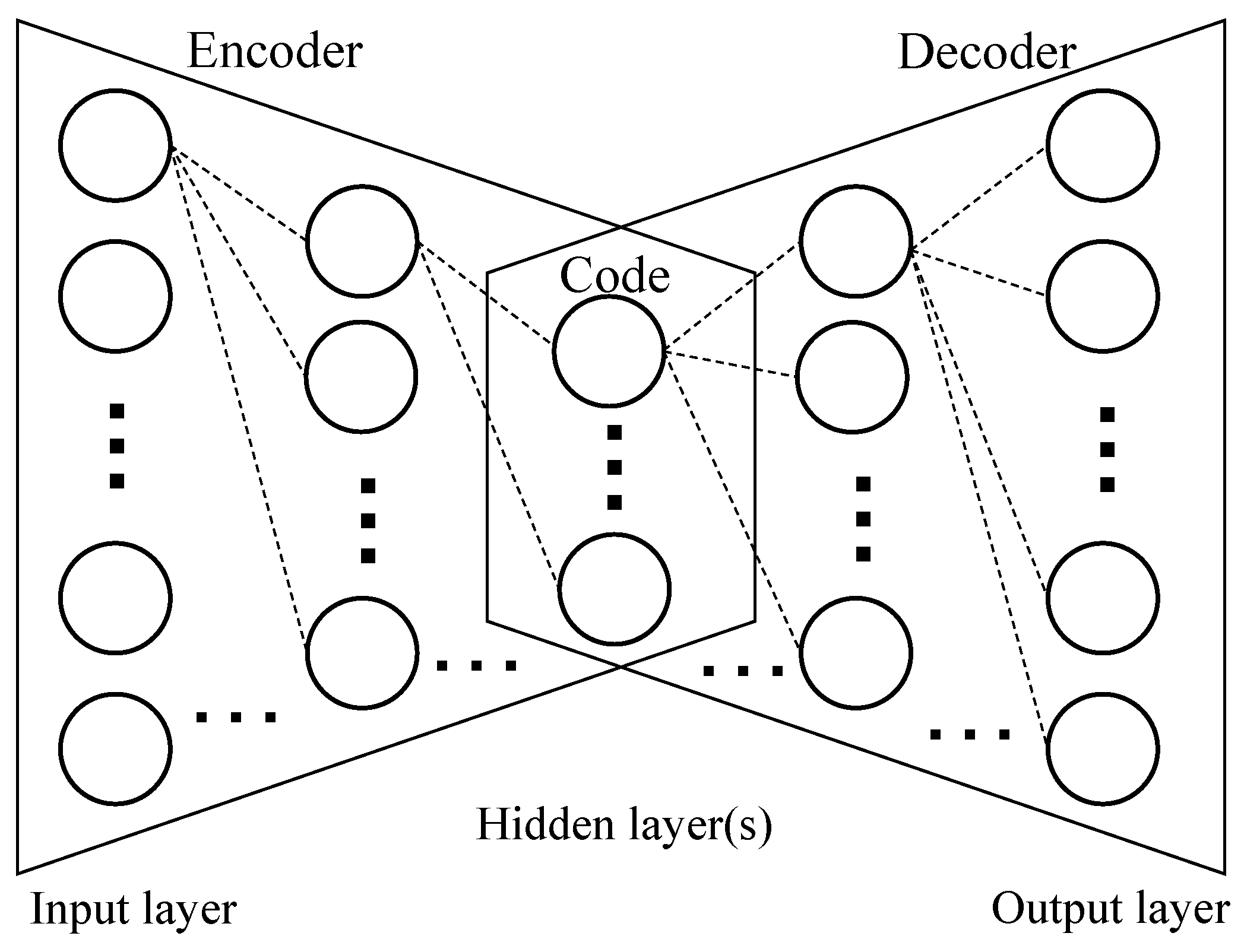
The neural network structure of an AE is symmetric, as shown in Figure 1. An AE has one input layer, one or more hidden layers, and one output layer. Especially, the output layer of an AE has the same number of neurons as the input layer. Furthermore, the kth hidden layer and the (n − k + 1)th hidden layer (or the kth hidden layer from the bottom) have the same number of neurons, where k = 1, …, ⌊n/2⌋, and n is the number of hidden layers. The middle hidden layer is called the bottleneck, and the states (values) of neurons in the bottleneck layer constitute the code or the latent representation of the input. The code can be regarded as the extracted feature or the dimensionality reduction result of the original input.

The first half part of an AE is called the encoder, whereas the second half part is called the decoder, as shown in Figure 1. The encoder encodes the input into the code, and the decoder decodes the code into the output. The output is intended to be as close to the input as possible; it is called the reconstructed input. The difference between the input and the output is called the reconstruction error. The AE is trained with the goal of minimizing the reconstruction errors by using the error backpropagation, gradient descent, and various optimizers like adaptive moment (Adam) optimizer.

2.2. Random Forest

The RF is an ensemble learning model for classification, regression, and other tasks [19]. Since the proposed AE-PRF method is for the task of classification, only the classification task is discussed in the following context. Specifically, the RF model utilizes decision trees to classify data and employs the bagging (i.e., bootstrap aggregating) approach to avoid the overfitting problem caused by complex decision trees. Below, the concept of using decision trees to classify data is first described.

A decision tree is a tree-like structure in which each internal node has a “split” based on an attribute, and each leaf node represents a prediction (or classification) result. Some metrics, such as the Gini impurity, entropy, and standard deviation, can be used for selecting the best splitting with the largest information gain. Below, the Gini impurity is taken as an example to show how the information gain is measured in decision trees. The information gain $IG\left(N_p, a\right)$ at node $N_p$ split into c child nodes $N_1, \dots , N_c$ based on the attribute a is defined in the following Equations (2) and (3):

$$IG\left(N_p, a\right)=Gini\left(N_p\right)-{\displaystyle \sum }_{i=1}^c\frac{\left|N_i\right|}{\left|N_p\right|}Gini\left(N_i\right)$$

(2)

$$Gini\left(N_p\right)=1-{\displaystyle \sum }_{j=1}^m{p}_j^2$$

(3)

In Equation (2), $\left|N_p\right|$ stands for the number of data at node $N_p$, and $\left|N_i\right|$ stands for the number of data at node $N_i$, 0 ≤ I ≤ c. In Equation (3), m is the number of different labels of data at node $N_p$, and $p_j$ is the ratio of the number of data with the jth label over the total number of data at node $N_p$.

The best splitting with the largest information gain is performed for every possible attribute and every possible attribute value of dividing. The splitting continues until one of the following three stop conditions occurs. The three stop conditions are (i) all data at a node have the same label, (ii) the number of data at a node reaches a pre-specified minimum limitation, and (iii) the depth of a node reaches a pre-specified maximum limitation. After the splitting stops, the decision trees can be used to classify an input sample. The input sample goes through the tree from the root node to a leaf node, and it is classified as the label that dominates others at the leaf node.

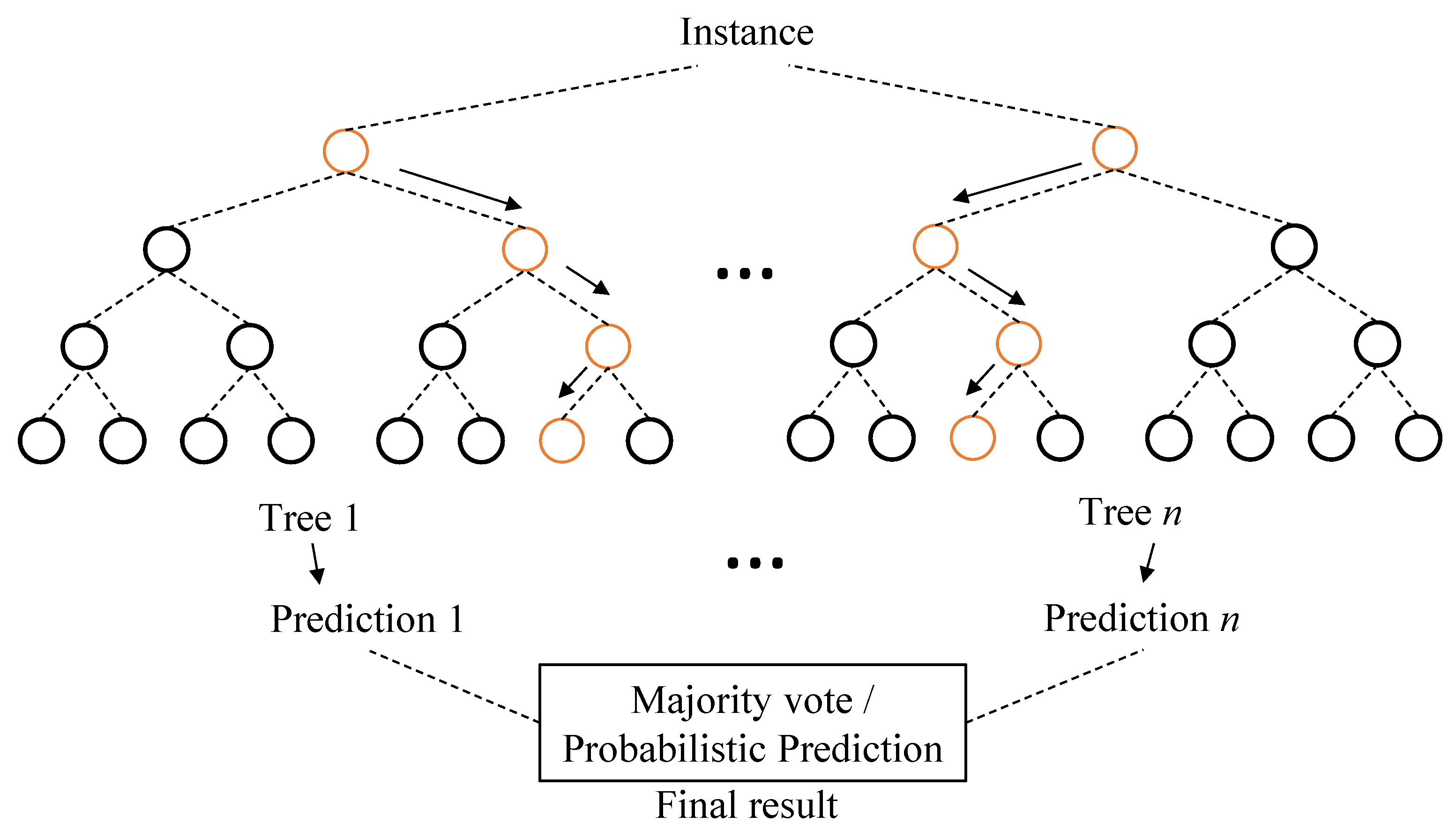
Below we describe the bagging approach that randomly selects partial data and partial attributes to construct a variety of decision trees to be combined for data classification. This can avoid the overfitting problem that is intrinsic in decision trees. Given a dataset of d data or observations, the bagging approach produces n sub-datasets by drawing d’ out of d observations with replacement, where d’ ≤ d. Every sub-dataset, along with a randomly selected subset of attributes, is used to train a decision tree. There are thus in total n decision trees that are trained independently with different sub-datasets and different attributes. Finally, either majority voting or averaging is applied to the n decision trees to get the final output of the RF, as shown in Figure 2.

In general, an RF model can be used to classify an input instance into one of r classes c₁, …, c_r. The procedure used to construct the RF model with n decision trees for a dataset of d data with k attributes has the following three major steps:

Step 1.

Produce n sub-datasets from the original dataset of d data. Each sub-dataset is produced by drawing d’ out of the d data with replacement, where d’ ≤ d.

Step 2.

For each of the n sub-datasets, grow a decision tree by choosing the best splitting of internal tree nodes with the largest information gain for arbitrary k’ attributes, k’ < k. There are thus in total n decision trees to generate n classifications, each of which is one of r classes (i.e., labels) c₁, …, c_r.

Step 3.

Aggregate the results of the n trees to output the dominant class $c_{out}=\arg {\max }_{i=1}^{r}freq\left(c_i\right)$ as the final classification, where $freq\left(c_i\right)$ is the frequency that c_i appears among the n classifications. Note that the output may be adjusted to be with probabilistic classification, i.e., to output the classification frequencies (or probabilities) freq(c₁), …, freq(c_r) for all classes c₁, …, c_r.

2.3. The Proposed AE-PRF Method

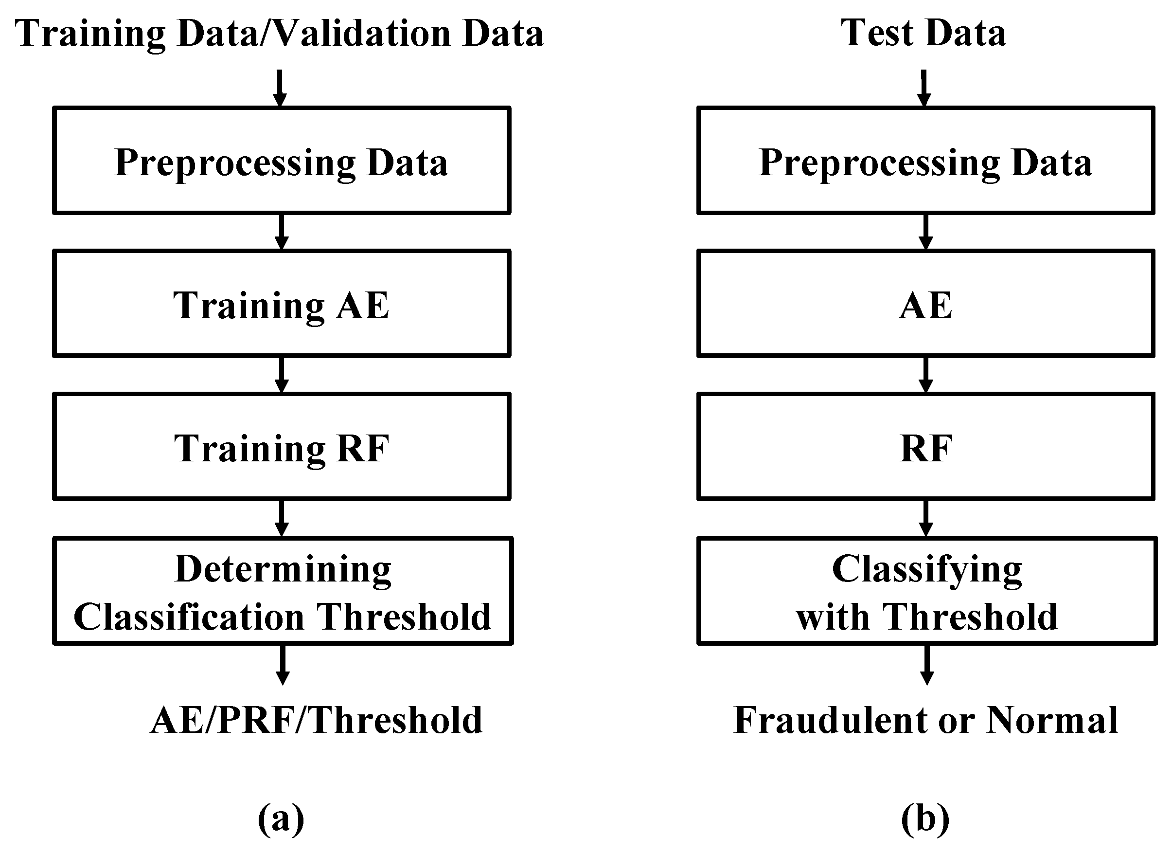
The proposed AE-PRF method first partitions the whole dataset as the training data, the validation data, and the test data. Figure 3 shows the processes of the proposed AE-PRF method. As shown in Figure 3, the data first undergo some preprocessing, and AE-PRF then applies the training data and the validation data to train an AE model. The AE model training is achieved by adjusting AE model weights properly with well-known error backpropagation and gradient descent mechanisms. The AE model can be used to reduce the data dimensionality and extract features from data as codes. Afterward, the codes of the training data are used to train an RF model to classify data into fraudulent data or normal data with associate classification probabilities. Moreover, the codes of the validation data are fed into the trained RF model to determine a proper threshold of classification probability to classify data with the best performance. Finally, for the verification purpose, the trained AE and RF models, along with the determined threshold can be applied to every test datum to check if it is fraudulent or normal.

Instead of directly using the RF model with a sole classification result, the AE-PRF method uses the RF model with probabilistic classifications to classify data. Specifically, the RF model with probabilistic classifications is used to classify a datum as fraudulent with probability p, and as normal with probability 1 − p, where 0 ≤ p ≤ 1. Afterward, AE-PRF outputs the final classification as fraudulent if p is larger than a pre-determined classification probability threshold θ. Different threshold values make AE-PRF generate different classification results. It is obvious that smaller θ values lead to a higher likelihood of classifying data as fraudulent. Fine-tuning the probability threshold θ value can provide AE-PRF with a customized classification result.

After the whole dataset is partitioned into the training data, the validation data, and the test data, the training process of AE-PRF can be started, as summarized in the following steps:

Step 1.

Employ the training data to train the AE model AET and obtain the set T of training data feature codes.

Step 2.

Train the RF model RFT with the set T of training data feature codes.

Step 3.

Apply AET to the validation data to extract the set V of validation data feature codes.

Step 4.

For threshold θ = 0 to 1 step s (=0.01), execute the following:

Feed every code in V into RFT to output a probability p of fraud classification. If p > θ, then the classification result is positive (fraudulent); otherwise, the classification result is negative (normal).

Step 5.

Employ the classification results of all codes in V to find the threshold value θ* producing the best classification performance in terms of a specific metric M.

After the above-mentioned AE-PRF training process is finished, the verification process can be started, as summarized in the following steps.

Step 1.

Apply AET to every test datum d to extract its feature code c.

Step 2.

Feed the code c into RFT with the threshold value θ* to produce the classification result of d.

The pseudocode the proposed AE-PRF method is shown as Algorithm 1 below. The source code of AE-PRF implementation can be found at https://github.com/LinTzuHsuan/AE-PRF (accessed on 10 October 2021).

Algorithm 1 AE-PRF

Input: training data Dtrain, validation data Dvalidation, test data Dtest, and metric M Output: the classification result of each test datum (0 for normal or 1 for fraudulent) 1: Train the AE model AET with Dtrain 2: T ← AET(Dtrain) 3: Train the RF model RFT with T 4: V ← AET(Dvalidation) 5: for θ ← 0 to 1 step 0.01 do 6:  for each v in V do 7:    p ← RFT(v) 8:    if p > θ then result [θ][v] ← 1 9:    else result [θ][v] ← 0 10: Find the best θ* by comparing all result values in terms of metric M 11: C ← AET(Dtest) 12: for each c in C do 13:  q ← RFT(c) 14:  if q > θ* then output [c] ← 1 15:  else output [c] ← 0 16: return output

3. Related Work

The methods proposed in [12,13,14,15] are most related to AE-PRF. They all use the CCFD dataset for performance evaluation. None of them undergo data resampling except the methods proposed in [12]. Below, the related methods are elaborated one by one.

Three credit card fraud detection methods, namely naïve Bayes (NB), k-nearest neighbor (k-NN), and logistic regression (LR), are proposed in [12]. The best classification result is achieved by the k-NN method with k = 3. The k-NN method is a non-parametric supervised machine learning algorithm that can be used for classification and regression [26]. A test datum is classified into the dominant class of its k nearest neighbors’ classes. Note that the random data resampling mechanism is adopted in [12] to address the data imbalance problem. Fraudulent data are oversampled and normal data are undersampled to make the ratio of fraudulent data to normal data 10:90 or 34:66 (≈1:2). The performance evaluation results show that data resampling can improve the performance of the k-NN method. However, it will be shown in this paper that data resampling does not necessarily improve the classification performance of the k-NN method.

Two unsupervised machine learning methods based on the AE model and the restricted Boltzmann machine (RBM) model are proposed in [13] for detecting credit card frauds. Like AE, RBM [27] can be sued to reconstruct input data. Both methods are unsupervised, as they need no data labels for training models. RBM can be regarded as a two-layer neural network with an input layer (visible) and a hidden layer. It is able to learn the probability distribution of the input data and thus can learn to reconstruct the data. This is achieved by fine-tuning the neural connection weights and biases through the processes of gradient descent and error back-propagation. For a new datum, either the trained AE or the trained RBM can be used to reconstruct the datum. The datum is assumed to be fraudulent if it has a large reconstruction error. As shown in [13], both AE and RBM have good fraud detection performance. However, AE is shown to have a better performance than RBM.

An unsupervised AE-based clustering method is proposed in [14] for detecting credit card frauds. The method uses an AE autoencoder with three hidden layers in both the encoder and the decoder. Moreover, it chooses the exponential linear unit (ELU) and the rectified linear unit (ReLU) as the activation functions of neurons in different layers. It also takes root mean square propagation (RMSProp) as the optimizer to yield the best result after performing several experiments. As shown in [14], the AE-base clustering method can achieve good classification performance by choosing an appropriate threshold of AE reconstruction errors to separate fraudulent data from normal data properly.

Twelve machine learning models for credit card fraud detection are studied in [15], including support vector machine (SVM) [28], naïve Bayes (NB), and feed-forward neural network (NN), etc. Furthermore, two ensemble learning mechanisms, namely adaptive boosting (AdaBoost) [29] and majority voting (MV), are combined with the twelve models to boost performance. Through comprehensive performance comparisons, SVM combined with AdaBoost (denoted as SVM + AdaBoost), and NN and NB combined with MV (denoted as NN + NB + MV) have comparably high performance. The SVM model generates a decision boundary in an increased or infinite-dimensional space, which is suitable for non-linear classification problems [30]. The AdaBoost method is an iterative method that adds a new weak classifier (i.e., classification model) in each iteration until all data are correctly classified, or the maximum iteration level has been reached. The NN + NB + MV model uses the feed-forward neural network and naïve Bayes concept [31] to perform fraud detection. The NN is an artificial neural network widely used in binary classification problems [32]. The NB is widely used for classification based on Bayes’ theorem with strong independence assumptions between features [33]. It is good for the cases that the independence assumption fits. Due to MV, the NN + NB + MV model yields good classification results even when data are added with 10% to 30% of noise.

4. Performance Evaluation and Comparisons

4.1. Dataset and Data Resampling

The CCFD dataset [22] contains data generated by European cardholders within 2 days in September 2013. It has a total of 284,807 transactions, among which 492 are fraudulent. The dataset is highly imbalanced because fraudulent data account for 0.172% of total data. Each data entry has 31 attributes, including the transaction timestamp, the transaction amount, and the transaction class or label, which is 1 if the transaction is fraudulent, and 0, otherwise. It also has 28 principal component analysis (PCA) transformation values of transaction data. The PCA values are transformed from transaction data. They are for the purpose of hiding information like the cardholder identity and personal privacy data. Note that PCA is a feature extraction mechanism to project high-dimensional data into low-dimensional data without losing crucial information. It can also be used to transform data for the purpose of data dimensionality reduction, data feature extraction, and data de-identification.

As mentioned earlier, in order to make the CCFD dataset more balanced, data resampling schemes such as SMOTE [23], ADASYN [24], and T-Link [25] are applied to CCFD data before they are fed into AE-PRF. The three schemes are used to balance the numbers of majority class samples (or majority samples, for short) and minority class samples (or minority samples, for short). Their basic ideas are described below.

SMOTE is an oversampling technique. For a minority sample x_i, SMOTE first finds k nearest minority samples based on the k-NN scheme. It then selects a sample x_j out of the k nearest minority samples and generates a new minority sample x_new according to the equation: $x_{new}=x_i+\delta \left(x_j-x_i\right)$, where $\delta ϵ \left[0,1\right]$. The process to generate new minority samples continues until the number of newly generated minority samples reaches the pre-specified value.

ADASYN is also an oversampling technique. It is similar to SMOTE, but it adaptively generates new minority samples for a minority sample according to its imbalance degree. Specifically, for a minority sample x_i, its k nearest samples are first derived and its imbalance degree is defined as Δ_i/k, where Δ_i is the number of majority samples out of the k nearest samples of x_i.

T-Link is an undersampling technique. It tries to find a pair of a minority sample x_i and a majority sample x_j such that there is no sample x_k satisfying d(x_k, x_j) < d(x_i, x_j) or d(x_i, x_k) < d(x_i, x_j), where d(u, v) is the Euclidean distance between samples u and v. It then removes the majority sample of every such pair so that the boundary between the majority class and the minority class is clearer and hence samples are easier to be classified.

4.2. Performance Metrics

The performance evaluation metrics, accuracy (ACC), the true positive rate (TPR), the true negative rate (TNR), and the false positive rate (FPR) are defined below in Equations (4)–(7), respectively.

$$\mathrm{ACC}=\frac{\mathrm{TP}+\mathrm{TN}}{\mathrm{TP}+\mathrm{TN}+\mathrm{FP}+\mathrm{FN}}$$

(4)

$$\mathrm{TPR}=\frac{\mathrm{TP}}{\mathrm{TP}+\mathrm{FN}}$$

(5)

$$\mathrm{TNR}=\frac{\mathrm{TN}}{\mathrm{TN}+\mathrm{FP}}$$

(6)

$$\mathrm{FPR}=\frac{\mathrm{FP}}{\mathrm{FP}+\mathrm{TN}}$$

(7)

In Equations (4)–(7), TP, FP, TN, and FN stand for the numbers of true positive, false positive, true negative, and false negative classifications (or predictions), respectively. A positive prediction is the one classifying a transaction as fraudulent, whereas a negative prediction is the one classifying a transaction as normal (i.e., not fraudulent). TP (respectively, FP) is the number of positive predictions for fraudulent (respectively, normal) transactions. TN (respectively, FN) is the number of negative predictions for normal (respectively, fraudulent) transactions. Note that TPR is also called sensitivity or recall, TNR is also called specificity, and FPR is also called the false alarm rate.

The area under the receiver operating characteristic curve (AUC) is a metric related to the receiver operating characteristic (ROC) curve. The ROC curve can be used as a tool to consider the tradeoff between TPR and FPR for a classifier based on threshold values. Different threshold values lead to different TPRs and FPRs. The ROC curve can be plotted by setting the x-axis as FPR and the y-axis as TPR, and the area under the ROC curve is then AUC. Larger AUC values correspond to better classifiers. If AUC has a value of 0.5, then the classifier is a no-skill classifier. If AUC has a value of 1, then the classifier is perfect.

The Matthews correlation coefficient (MCC) [34], as defined in Equation (8), can be regarded as a comprehensive metric, since it addresses TP, FP, TN, and FN at the same time. MCC has values within the range between −1 and +1, where the value of +1 indicates perfect predictions and −1 means entirely conflicting predictions. As stated in [35], MCC is suitable for both balanced and imbalanced datasets. Therefore, in the following performance evaluation, we consider MCC as an important metric.

$$\mathrm{MCC}=\frac{\mathrm{TP}\times \mathrm{TN}-\mathrm{FP}\times \mathrm{FN}}{\sqrt{\left(\mathrm{TP}+\mathrm{FP}\right)\left(\mathrm{TP}+\mathrm{FN}\right)\left(\mathrm{TN}+\mathrm{FP}\right)\left(\mathrm{TN}+\mathrm{FN}\right)}}$$

(8)

Several evaluation metrics, including ACC, TPR, TNR, MCC, AUC, recall, F1-score, log loss/binary cross-entropy, and categorical cross-entropy, can be used for evaluating the performance of classification methods. Among them, ACC, TPR, TNR, and MCC, which are defined in Equations (4)–(6) and (8), as well as AUC are commonly used for evaluating the performance of credit card fraud detection methods [12,13,14,15]. Specifically, the two most important metrics are TPR and MCC. The reason for the first metric, TPR, to be adopted in fraud detection is that the higher the TPR, the more fraudulent data can be detected, which is the main purpose of fraud detection. However, when evaluating the averaging performance of a model, MCC would be considered, because it takes every parameter including TP, TN, FP, and FN into consideration. To sum up, ACC, TPR, TNR, MCC, and AUC are deployed as metrics for performance evaluations and comparisons.

4.3. Performance Evaluation of AF-PRF

To evaluate the performance of the proposed AE-PRF method, the CCFD dataset is first partitioned into a training dataset of 64% data, a validation dataset of 16% data, and a test dataset of 20% data. All data undergo pre-processing such as the logarithmic transform on the amount of transaction and the second-to-day transform on the number of seconds elapsed between the transaction and the first transaction in the dataset. The hyper-parameters of AE-PRF are described as follows. The AE model has five hidden layers with 26, 20, 18, 20, and 26 neurons, respectively, using the rectified linear unit (ReLU) as the activation function. The AE model uses the Adam as the optimizer, except for the first layer, using hyperbolic tangent (Tanh) instead. In order to prevent overfitting, L1 Regularization is applied to the first layer of the encoder. At the training stage, early stopping is adopted to prevent overfitting, using validation loss as the monitor. The dimension of the CCFD dataset data is reduced from 26 attributes to 18 by the trained AE. Well-defined feature extraction and dimensionality reduction algorithms (e.g., the AE model) make the detection/classification process more effective and efficient. The most important and influential features of the data will be focused on after dimensionality reduction.

The RF model of AE-PRF has 100 decision trees (estimators) and uses Gini impurity as the criterion, as defined in Equation (3). It generates probabilistic classification, i.e., it classifies the test datum as fraudulent with probability p, 0 ≤ p ≤ 1.

The AE-PRF performance evaluation has two parts. The first part does not apply resampling mechanisms to data, whereas the second part applies resampling mechanisms to data. Below, we first describe the first part.

As mentioned earlier, AE-PRF uses the RF model with probabilistic classification with probability p to check if a test datum is classified as fraudulent. If p is larger than a pre-specified classification threshold θ, then the test datum is assumed to be fraudulent. Certainly, different threshold values lead to different classification performances. In order to find the best threshold confronting different requirements, it is necessary to fine-tune and shift the threshold and find the one which produces the best result in terms of specific metrics. More specifically, fine-tuning the threshold by testing different threshold values 0, 0.01, 0.02, …, 1 in agreement with the evaluation metric is the way to find the best threshold.

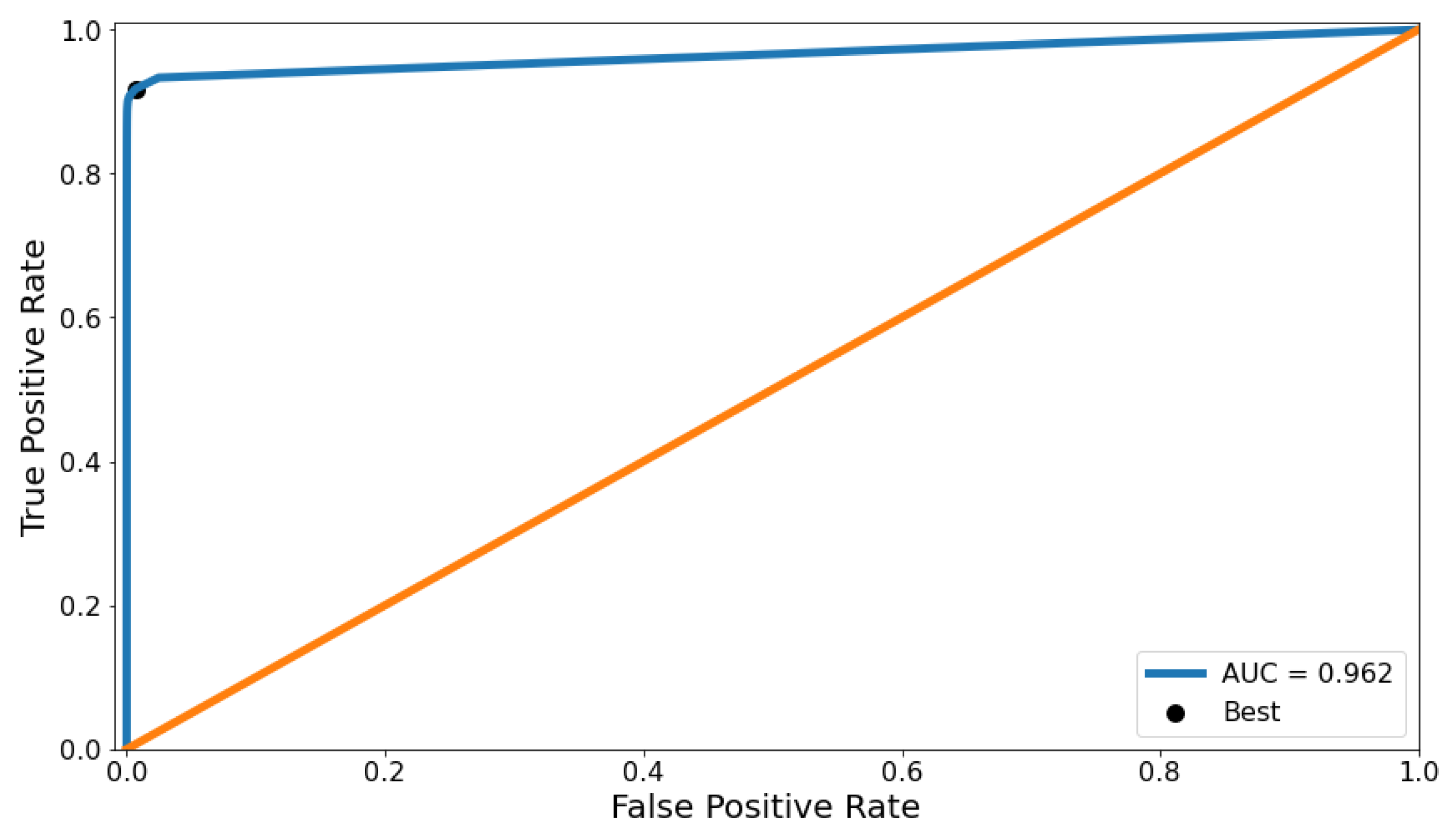
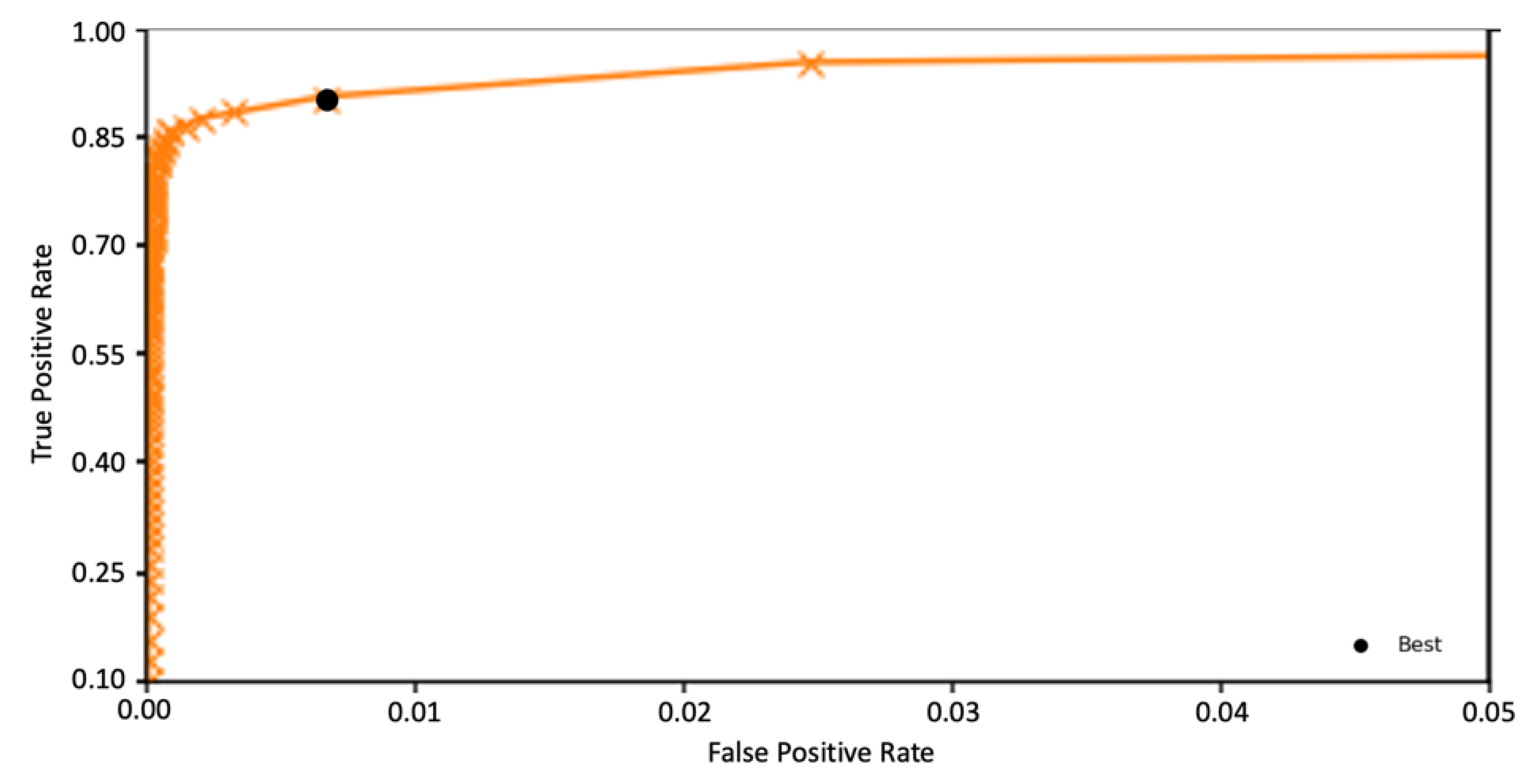
The threshold is first obtained by the ROC curve. To be precise, 101 different threshold θ values are applied to the AE-PRF classifier, ranging from 0 to 1 with the step interval of 0.01. Experiments are conducted 50 times to derive the average TPR and FPR, which in turn are used to plot the ROC curve, as shown in Figure 4. The zoomed-in version of Figure 4 is also given in Figure 5. We randomly repartitioned the dataset into a training set, a validation set, and a test set, and repeat the experiment 50 times to reduce biases of experimental results. The diagonal line in Figure 4 indicates the curve for a no-skill classifier. The upper left point on the ROC curve in Figure 4 indicates a model with perfect skill, which is computed by the geometric mean (or g-mean) of TPR and FPR (i.e., $\sqrt{\mathrm{TPR}\times \left(1-\mathrm{FPR}\right)}$. The g-mean of TPR and FPR is a good indicator of classification for imbalanced data. When it is optimized, a balance between the sensitivity (i.e., TPR) and specificity (i.e., TNR) is reached. The threshold recommended by the ROC curve is 0.03, which is the one corresponding to the best g-mean. The AUC of the ROC curve is 0.962, which is better than 0.960 of the method proposed in [13] and 0.961 of the method proposed in [14].

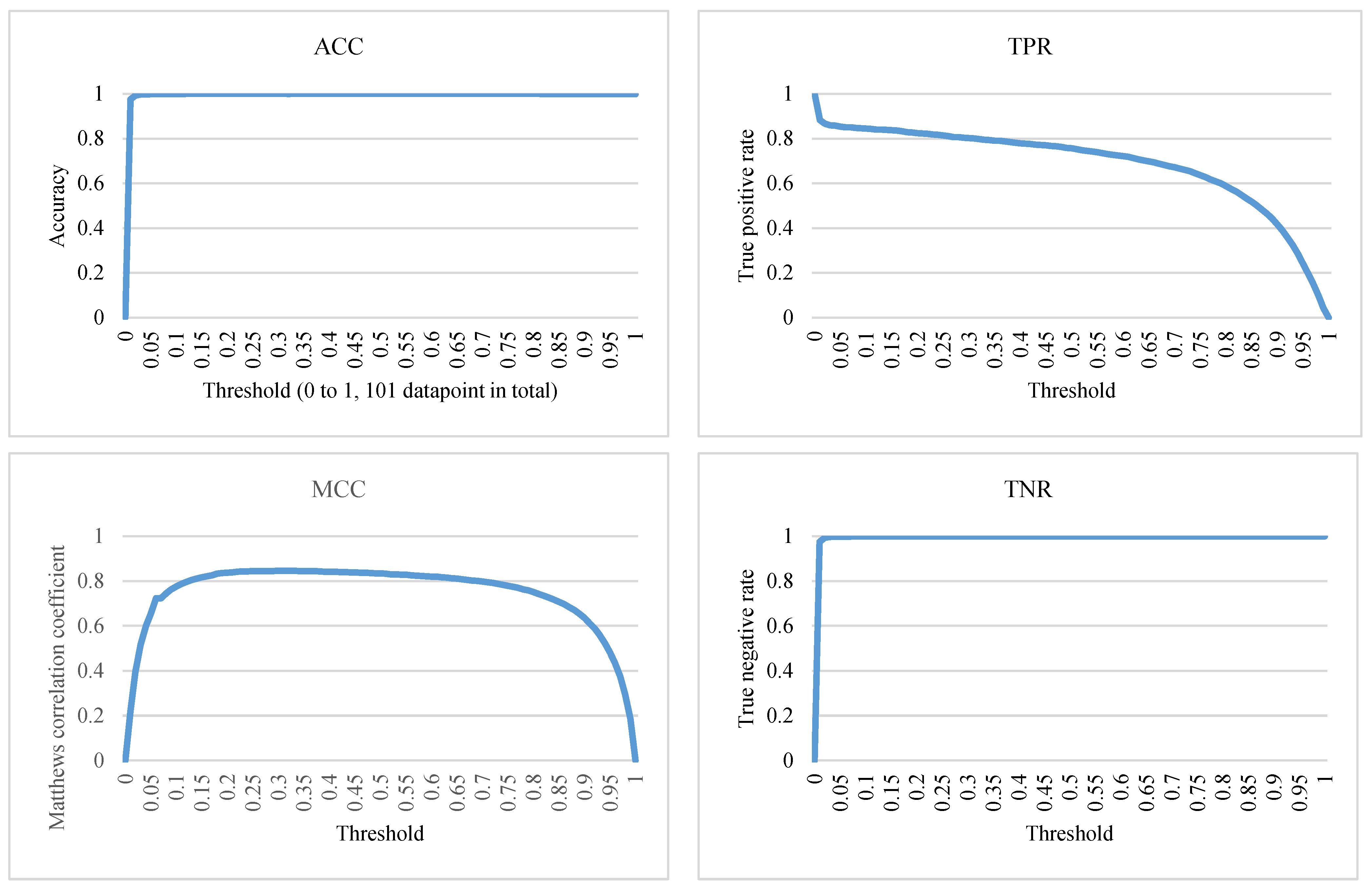
Similarly, the threshold is then tuned to obtain the best ACC, TPR, TNR, and MCC, as demonstrated in Figure 6. The ACC is very high with 101 thresholds, all about 0.99, except for θ = 0. However, a high ACC alone cannot be interpreted as this fraud detection classifier being good enough. When dealing with highly imbalanced datasets, it is common to get a high ACC [36]. Therefore, other evaluation metrics must be taken into consideration. As for TNR, it also gets high scores with most of the thresholds, and the highest score is around 0.9998 achieved by θ = 0.25. However, for the same reason as the ACC metric, because datasets of fraud detection problems are usually highly imbalanced, it tends to obtain a much higher TN value than FP value, which easily results in a high TNR [37].

Therefore, this study considers MCC as a very important metric. Specifically, when considering and choosing the optimal threshold, this study just focuses on the thresholds generating MCC scores that are greater than 0.8. Thus, only threshold values ranging from 0.13 to 0.69 are considered. Consequently, the best average MCC is around 0.8456, obtained by setting θ = 0.25.

However, it is risky to consider only one metric. In the credit card fraud detection problem, it is desirable to achieve higher TPRs so that more fraudulent data can be detected [36]. Nonetheless, if there are no restrictions, the highest TPR will always be achieved by θ = 0. Under such a setting, not only ACC and TNR but also MCC will be very low, being 0. Thus, here, the premise is to set MCC greater than 0.5 and find the best TPR. In other words, if we want to detect as many fraudulent transactions as possible while maintaining a decent overall performance, another threshold must be adopted. To the best of our knowledge, the TPR of 0.89109 achieved by setting θ as 0.03 is the highest one ever seen while keeping MCC greater than 0.5. Note that setting θ as 0.03 is also recommended by the ROC curve using the g-mean of TPR and FPR.

Table 1. Performance of AE-PRF in 50 times of experiments (θ = 0.25).

Metrics	Average	Minimum	Q1	Q2	Q3	Maximum
ACC	0.99949	0.999410129	0.999455774	0.999494396	0.999522485	0.999578664
TPR	0.8142	0.75	0.808333333	0.816666667	0.825	0.84166667
TNR	0.9998	0.999704567	0.999788976	0.999803044	0.999831181	0.999887454
MCC	0.8441	0.811201026	0.834295395	0.845629405	0.853475139	0.870180134

shows the details of performance metrics of AE-PRF for θ = 0.25, which yields the best average MCC in our experiments. The details are the average score, the lowest scores (Minimum), the first quartile (Q1), the second quartile (Q2), the third quartile (Q3), and the highest scores (Maximum) of ACC, TPR, TNR, and MCC in 50 experiments with θ = 0.25. The average score will be compared with those of other related methods later.

Now, the second part of the AE-PRF performance evaluation is described. In this part, ADASYN itself and the combination of SMOTE and T-Link, denoted as SMOTE + T-Link, were applied to the training dataset for resampling data to make them more balanced. This was to verify whether the use of data resampling techniques can improve AE-PRF performance. However, if data resampling does not noticeably improve AE-PRF performance, then AE-PRF is said to be naturally suitable for dealing with imbalanced data.

The performance evaluation results of the AE-PRF without data resampling and with ADASYN and SMOTE + T-Link data resampling are shown in

Table 2. Performance of AE-PRF with and without data resampling.

Models	ACC	TPR	TNR	MCC
AE-PRF (θ = 0.03)	0.9973	0.8910	0.9975	0.5921
AE-PRF (θ = 0.25)	0.9995	0.8142	0.9998	0.8441
ADASYN AE-PRF (θ = 0.13)	0.9960	0.8613	0.9963	0.5018
ADASYN AE-PRF (θ = 0.57)	0.9995	0.8316	0.9998	0.8665
SMOTE + T-Link AE-PRF (θ = 0.11)	0.9965	0.8583	0.9967	0.5133
SMOTE + T-Link AE-PRF (θ = 0.51)	0.9995	0.8333	0.9998	0.8585

. The sampling strategies of ADASYN and SMOTE + T-Link are the same. That is, the ratio of the minority sample quantity over the majority sample quantity is set to 34:66 (≈1:2) for both ADASYN and SMOTE + T-Link. Specifically, both ADASYN and SMOTE + T-Link adjust the number of fraudulent transactions to be 142,172, and the number of normal transactions to be 284,315 for the training dataset. As observed from Table 2, the performance of AE-PRF is not noticeably improved by data resampling. Moreover, AE-PRF using no data resampling even has better performance than AE-PRF using data resampling in terms of some metrics. It thus may be proper to say that AE-PRF is naturally suitable for dealing with imbalanced data.

4.4. Perforamance Comparisons

Here, after several experiments, θ is set to be of values 0.25 and 0.03 for comparing AE-PRF and five related methods in terms of various performance metrics to demonstrate the superiority of AE-PRF. The five methods are the k-NN [12], AE [13], AE based clustering [14], SVM + AdaBoost [15], and NN + NB with MV [15]. All methods for comparison, including the proposed AE-PRF, use no data sampling. The performance comparisons were performed in terms of ACC, TPR, TNR, AUC, and MCC.

Table 3. Performance comparisons of AE-PRF and related methods.

Research	Methods	ACC	TPR	TNR	MCC	AUC
Awoyemi et al. [12]	k-NN	0.9691	0.8835	0.9711	0.5903	-
Pumsirirat et al. [13]	AE	0.97054	0.83673	0.97077	0.1942	0.9603
Zamini et al. [14]	AE-based clustering	0.98902	0.81632	0.98932	0.3058	0.961
Randhawa et al. [15]	SVM with AdaBoost	0.99927	0.82317	0.99957	0.796	-
Randhawa et al. [15]	NN+NB with MV	0.99941	0.78862	0.99978	0.823	-
This Research	AE + PRF (θ = 0.03)	0.99738	0.89109	0.99757	0.5921	0.962
This Research	AE + PRF (θ = 0.25)	0.9995	0.8142	0.9998	0.8441	0.962

shows the performance comparison results of AE-PRF and other five related methods. The highest scores in Table 3 are in boldface. It can be seen that AE-PRF outperformed others in almost all metrics. As for AE-PRF with θ = 0.25, it had the highest ACC of 0.9995, the highest TNR of 0.9998, and the highest MCC of 0.8441. However, its TPR of 0.8142 was lower than the highest score of 0.8835 achieved by k-NN [12]. Therefore, another threshold was adopted, AE-PRF with θ = 0.03 had the highest TPR of 0.89109 and comparable high ACC, TNR, and MCC. If the main goal of the credit card fraud detection is to achieve as high TPR as possible while maintaining a decent MCC (say ≥ 0.5), then AE-PRF with θ = 0.03 is the best one to choose.

Note that the k-NN method proposed in [12] has two versions, one using data resampling and the other using no data resampling. However, only the version using no data resampling is compared with the proposed AE-PRF method in Table 3. This is because when we re-implement the k-NN method and apply random data resampling to the re-implemented k-NN method, the performance of the re-implemented k-NN does not conform with the performance results shown in [12]. As demonstrated in

Table 4. Performance of k-NN [12] and re-implemented k-NN with and without data resampling.

Methods	ACC	TPR	TNR	MCC
k-NN [12] (without resampling)	0.9691	0.8835	0.9711	0.5903
k-NN [12] (with all data 34:66 resampling)	0.9792	0.9375	1.0	0.9535
Re-implemented k-NN (without resampling)	0.9977	0.7483	0.9981	0.5512
Re-implemented k-NN (with only training data resampling)	0.9817	0.1881	0.9832	0.0556
Re-implemented k-NN (with all data 34:66 resampling)	0.9832	0.9494	1.0	0.9624

, the data resampling even makes k-NN have bad performance. The research [12] likely applied data resampling to the whole data, including the training and the test data, whereas we apply data resampling to only the training data. We confirm this by applying random data resampling to the whole data and then running the re-implemented k-NN method. As observed from Table 4, if the whole data is resampled, then the performance results of the original k-NN and the re-implemented k-NN are quite similar. However, not all test data can be obtained in advance and each test datum should be classified separately. Resampling all data, including training data and test data, seems to be impractical.

5. Conclusions

This paper proposes a fraud detection method called AE-PRF. It employs AE to reduce data dimensionality and extract data features. Moreover, it utilizes RF with probabilistic classification to classify data as fraudulent along with an associated probability. AE-PRF outputs the final classification as fraudulent if the associated probability exceeds a pre-determined probability threshold θ.

The CCFD dataset [22] was applied to evaluate the performance of AE-PRF. Since the CCFD dataset is highly imbalanced, data resampling schemes like SMOTE [23], ADASYN [24], and T-Link [25] were applied to the CCFD dataset to balance the numbers of normal and fraudulent transactions. Experimental results showed that the performance of AE-PRF does not vary much whether resampling schemes are applied to the dataset or not. This indicates that AE-PRF is naturally suitable for handling imbalanced datasets without data resampling.

The performance evaluation results of AE-PRF without data resampling were compared with those of related methods such as k-NN [12], AE [13], AE-based clustering [14], SVM with AdaBoost [15], and NN + NB with MV [15]. The comparison results show that AE-PRF with θ = 0.25 has the highest ACC, TNR, MCC, and AUC, and has comparably high TPR. As for AE-PRF with θ = 0.03, it has the highest TPR and AUC, and comparable high ACC, TNR, and MCC. The CCFD dataset is partitioned into a training dataset of 64% data, a validation dataset of 16% data, and a test dataset of 20% data for evaluating AE-PRF performance. We tried another extreme partition, a training dataset of 40% data, a validation dataset of 10% data, and a test dataset of 50%, which does not yield a good result because of the insufficient training data.

It is more persuasive to compare AE-PRF to existing methods using the same dataset for performance evaluation. Since the CCFD dataset was adopted by many existing methods and it is the most detailed public dataset, this paper adopted the CCFD dataset for performance evaluation and comparison. However, in order to test the robustness and effectiveness of AE-PRF, we need to adopt some other datasets, especially private datasets, because there are few public datasets for credit card fraud detection due to privacy issues. In the future, we plan to cooperate with credit card issuers and/or banks to obtain datasets for verifying the robustness and the effectiveness of AE-PRF.

In the future, we will try to improve AE-PRF performance by fine-tuning the hyperparameters of the AE and the RF models. We will also try to apply AE-PRF to a variety of applications for evaluating AE-PRF’s applicability. Furthermore, we will investigate the explainability of AE-PRF and try to enhance AE-PRF’s explainability by leveraging novel explainable AI (XAI) schemes proposed in [38,39,40] for AE and RF.

References

- de Best, R. Credit Card and Debit Card Number in the U.S. 2012–2018. Statista. 2020. Available online: https://www.statista.com/statistics/245385/number-of-credit-cards-by-credit-card-type-in-the-united-states/#statisticContainer (accessed on 10 October 2021).
- Voican, O. Credit Card Fraud Detection using Deep Learning Techniques. Inform. Econ. 2021, 25, 70–85. [Google Scholar] [CrossRef]
- The Nilson Report. Available online: https://nilsonreport.com/mention/1313/1link/ (accessed on 20 December 2020).
- Taha, A.A.; Sharaf, J.M. An intelligent approach to credit card fraud detection using an opti-mized light gradient boosting machine. IEEE Access 2020, 8, 25579–25587. [Google Scholar] [CrossRef]
- Dal Pozzolo, A. Adaptive Machine Learning for Credit Card Fraud Detection. Ph.D. Thesis, Université Libre de Bruxelles, Brussels, Belgium, 2015. [Google Scholar]
- Lucas, Y.; Portier, P.-E.; Laporte, L.; Calabretto, S.; Caelen, O.; He-Guelton, L.; Granitzer, M. Multiple perspectives HMM-based feature engineering for credit card fraud detection. In Proceedings of the 34th ACM/SIGAPP Symposium on Applied Computing, ACM, New York, NY, USA, 8–12 April 2019; pp. 1359–1361. [Google Scholar]
- Wiese, B.; Omlin, C. Credit Card Transactions, Fraud Detection, and Machine Learning: Modelling Time with LSTM Recurrent Neural Networks. In Studies in Computational Intelligence; Springer Science and Business Media LLC: Berlin, Germany, 2009; pp. 231–268. [Google Scholar]
- Jurgovsky, J.; Granitzer, M.; Ziegler, K.; Calabretto, S.; Portier, P.-E.; He-Guelton, L.; Caelen, O. Sequence classification for credit-card fraud detection. Expert Syst. Appl. 2018, 100, 234–245. [Google Scholar] [CrossRef]
- Zhang, F.; Liu, G.; Li, Z.; Yan, C.; Jiang, C. GMM-based Undersampling and Its Application for Credit Card Fraud Detection. In Proceedings of the 2019 International Joint Conference on Neural Networks (IJCNN), Budapest, Hungary, 14–19 July 2019; pp. 1–8. [Google Scholar]
- Ahammad, J.; Hossain, N.; Alam, M.S. Credit Card Fraud Detection using Data Pre-processing on Imbalanced Data—Both Oversampling and Undersampling. In Proceedings of the International Conference on Computing Advancements, New York, NY, USA, 10–12 January 2020; ACM Press: New York, NY, USA, 2020. [Google Scholar]
- Lee, Y.-J.; Yeh, Y.-R.; Wang, Y.-C.F. Anomaly Detection via Online Oversampling Principal Component Analysis. IEEE Trans. Knowl. Data Eng. 2012, 25, 1460–1470. [Google Scholar] [CrossRef] [Green Version]
- Awoyemi, J.O.; Adetunmbi, A.O.; Oluwadare, S.A. Credit card fraud detection using machine learning techniques: A comparative analysis. In Proceedings of the 2017 International Conference on Computing Networking and Informatics (ICCNI), Lagos, Nigeria, 29–31 October 2017; pp. 1–9. [Google Scholar]
- Pumsirirat, A.; Yan, L. Credit Card Fraud Detection using Deep Learning based on Auto-Encoder and Restricted Boltzmann Machine. Int. J. Adv. Comput. Sci. Appl. 2018, 9, 18–25. [Google Scholar] [CrossRef]
- Zamini, M.; Montazer, G. Credit Card Fraud Detection using autoencoder based clustering. In Proceedings of the 2018 9th International Symposium on Telecommunications (IST), Tehran, Iran, 17–19 December 2018; pp. 486–491. [Google Scholar] [CrossRef]
- Randhawa, K.; Loo, C.K.; Seera, M.; Lim, C.P.; Nandi, A.K. Credit Card Fraud Detection Using AdaBoost and Majority Voting. IEEE Access 2018, 6, 14277–14284. [Google Scholar] [CrossRef]
- Lucas, Y.; Johannes, J. Credit card fraud detection using machine learning: A survey. arXiv 2020, arXiv:2010.06479. [Google Scholar]
- Nikita, S.; Pratikesh, M.; Rohit, S.M.; Rahul, S.; Chaman Kumar, K.M.; Shailendra, A. Credit card fraud detection techniques—A survey. In Proceedings of the 2020 International Conference on Emerging Trends in Information Technology and Engineering, Vellore, India, 24–25 February 2020. [Google Scholar]
- Rumelhart, D.E.; Geoffrey, E.H.; Ronald, J.W. Learning internal representations by error propagation. Calif. Univ. San Diego La Jolla Inst. Cogn. Sci. 1985, 8, 318–362. [Google Scholar]
- Liaw, A.; Matthew, W. Classification and regression by random Forest. R News 2002, 2, 18–22. [Google Scholar]
- Seeja, K.R.; Zareapoor, M. FraudMiner: A Novel Credit Card Fraud Detection Model Based on Frequent Itemset Mining. Sci. World J. 2014, 2014, 1–10. [Google Scholar] [CrossRef]
- Zhang, C.; Gao, W.; Song, J.; Jiang, J. An imbalanced data classification algorithm of improved autoencoder neural network. In Proceedings of the 2016 Eighth International Conference on Advanced Computational Intelligence (ICACI), Chiang Mai, Thailand, 14–16 February 2016; pp. 95–99. [Google Scholar]
- Credit Card Fraud Detection Dataset. Available online: https://www.kaggle.com/mlg-ulb/creditcardfraud (accessed on 20 August 2020).
- Chawla, N.V.; Bowyer, K.W.; Hall, L.O.; Kegelmeyer, W.P. SMOTE: Synthetic Minority Over-sampling Technique. J. Artif. Intell. Res. 2002, 16, 321–357. [Google Scholar] [CrossRef]
- He, H.; Bai, Y.; Garcia, E.A.; Li, S. ADASYN: Adaptive synthetic sampling approach for imbalanced learning. In Proceedings of the IEEE International Joint Conference on Neural Networks, Hong Kong, China, 1–8 June 2008; pp. 1322–1328. [Google Scholar] [CrossRef] [Green Version]
- Tomek, I. Two Modifications of CNN. IEEE Trans. Syst. Man Cybern. 1976, 6, 769–772. [Google Scholar] [CrossRef] [Green Version]
- Altman, N.S. An introduction to kernel and nearest-neighbor nonparametric regression. Am. Stat. 1992, 46, 175–185. [Google Scholar]
- Sutskever, I.; Geoffrey, E.H.; Graham, W.T. The recurrent temporal restricted boltzmann machine. In Advances in Neural Information Processing Systems; University of Toronto: Toronto, ON, Canada, 2009. [Google Scholar]
- Bhattacharyya, S.; Jha, S.; Tharakunnel, K.; Westland, J.C. Data mining for credit card fraud: A comparative study. Decis. Support Syst. 2011, 50, 602–613. [Google Scholar] [CrossRef]
- Margineantu, D.; Dietterich, T. Pruning Adaptive Boosting. In Proceedings of the 14th International Conference on Machine Learning, ICML, Guangzhou, China, 18–21 February 1997. [Google Scholar]
- Naveen, P.; Diwan, B. Relative Analysis of ML Algorithm QDA, LR and SVM for Credit Card Fraud Detection Dataset. In Proceedings of the 2020 Fourth International Conference on I-SMAC (IoT in Social, Mobile, Analytics and Cloud) (I-SMAC), Palladam, India, 7–9 October 2020; pp. 976–981. [Google Scholar]
- Rish, I. An Empirical Study of the Naive Bayes Classifier. In Proceedings of the IJCAI 2001 Workshop on Empirical Methods in Artificial Intelligence. 2001, Volume 3. No. 22. Available online: https://www.cc.gatech.edu/fac/Charles.Isbell/classes/reading/papers/Rish.pdf (accessed on 20 August 2020).
- Jeatrakul, P.; Wong, K.W. Comparing the performance of different neural networks for binary classification prob-lems. In Proceedings of the 2009 Eighth International Symposium on Natural Language Processing, Bangkok, Thailand, 20–22 October 2009. [Google Scholar]
- Murphy, K.P. Naive Bayes Classifiers; University of British Columbia: Vancouver, BC, Canada, 2006. [Google Scholar]
- Chicco, D.; Jurman, G. The advantages of the Matthews correlation coefficient (MCC) over F1 score and accuracy in binary classification evaluation. BMC Genom. 2020, 21, 1–13. [Google Scholar] [CrossRef] [PubMed] [Green Version]
- Saito, T.; Rehmsmeier, M. The Precision-Recall Plot Is More Informative than the ROC Plot When Evaluating Binary Classifiers on Imbalanced Datasets. PLoS ONE 2015, 10, e0118432. [Google Scholar] [CrossRef] [PubMed] [Green Version]
- Chawla, N.V. Data Mining for Imbalanced Datasets: An Overview. Data Min. Knowl. Discov. Handb. 2009, 875–886. [Google Scholar] [CrossRef] [Green Version]
- Lakshmi, T.J.; Prasad, C.S.R. A study on classifying imbalanced datasets. In Proceedings of the 2014 First International Conference on Networks & Soft Computing (ICNSC2014), Guntur, India, 19–20 August 2014; pp. 141–145. [Google Scholar]
- Assaf, R.; Giurgiu, I.; Pfefferle, J.; Monney, S.; Pozidis, H.; Schumann, A. An Anomaly Detection and Explainability Framework using Convolutional Autoencoders for Data Stor-age Systems. IJCAI 2020, 5228–5230. [Google Scholar] [CrossRef]
- Antwarg, L.; Miller, R.M.; Shapira, B.; Rokach, L. Explaining anomalies detected by autoencoders using Shapley Additive Explanations. Expert Syst. Appl. 2021, 186, 115736. [Google Scholar] [CrossRef]
- Fernández, R.R.; de Diego, I.M.; Aceña, V.; Fernández-Isabel, A.; Moguerza, J.M. Random forest explainability using counterfactual sets. Inf. Fusion 2020, 63, 196–207. [Google Scholar] [CrossRef]
Publisher’s Note: MDPI stays neutral with regard to jurisdictional claims in published maps and institutional affiliations. |
© 2021 by the authors. Licensee MDPI, Basel, Switzerland. This article is an open access article distributed under the terms and conditions of the Creative Commons Attribution (CC BY) license (https://creativecommons.org/licenses/by/4.0/).