Abstract
The pressing process is a part of the fabrication process of multi-layer printed circuit board (PCB) manufacturing. This paper presents the application of a new mixed-integer linear programming model to the short-term scheduling of the pressing process. The objective was to minimize the makespan. The proposed model is an improvement from our previous model in the literature. The size complexity of the proposed model is better than that of the previous model, whereby the number of variables, constraints, and the dimensionality of variables in the previous model are reduced. To compare their performance, problems from literature and additional generated test problems were solved. The proposed model was shown to outperform the previous model in terms of computational complexity. It can verify a new optimal solution for some problems. For the problems that could not be solved optimally, the proposed model could find the incumbent solution using much less computational time than the previous model, and the makespan of the incumbent solution from the proposed model was better than or equal to that of the previous model. The proposed model can be a good option to provide an optimal schedule for the pressing process in any PCB industry.
1. Introduction
Printed circuit boards (PCBs) are used as a major component in most electronic devices [1]. Nowadays, most PCB manufacturers are facing the challenge of improving production efficiency to cope with the strong competition [2]. In every aspect of production, the productivity and cost are crucial matters. Reducing the production cost whilst maximizing the efficiency of the production machines are the prime objectives of a manufacturing enterprise.
PCBs can be classified into three types, according to the number of their layers, as single-layer PCBs, double-layer PCBs, and multi-layer PCBs. This paper only considers multi-layer PCBs. Multi-layer PCB manufacturing consists of the design, fabrication, assembly, and testing [3]. The design step is creating a circuit schematic by PCB designers. The fabrication step is creating the PCB or bare board. There are many processes in multi-layer PCB fabrication, such as cutting, pressing, and drilling processes. The assembly step is the placing of electronic components at the predefined positions on the bare board. Lastly, the testing step identifies early fallouts before the PCBs are sent for use in the field.
This paper focuses on the pressing process in multi-layer PCB fabrication, which involves various PCB components and costly machines. Scheduling an efficient pressing process requires backgrounds in assignment and sequencing to reduce the production time and to increase machine utilization. The mathematical problems in the literature that have similar backgrounds to the pressing process (assignment and sequencing) are the flexible job shop scheduling problem (FJSP) [4,5,6,7] and the hybrid flow shop scheduling problem (HFSP) [8,9]. However, literature about pressing process scheduling is quite limited. To the best of the authors’ knowledge, there is no prior work that directly investigated pressing process scheduling, except the authors’ prior publication [10], where a mixed integer linear programming (MILP) model and a heuristic algorithm were used for solving the pressing process scheduling. The objective of pressing process scheduling is to minimize makespan. The test problems generated from the data of an actual PCB company were solved using both methods to show the performance.
Although approximate methods, such as a heuristic algorithm, can solve an optimization problem within a relatively short time, it can be difficult to guarantee the quality of the solution to the problem. The first key step to study an optimization problem is to mathematically formulate it. A mathematical programming model is the first natural way to approach a scheduling problem [8,11]. It can explicitly describe the objective, constraints, and all the other characteristics of the scheduling problem. Moreover, it can serve as the key to develop a heuristic algorithm for solving the problem [12]. The MILP is a type of mathematical programming model that allows an exact method to solve a scheduling problem and gives an optimal solution if one exists. Therefore, it is important to improve the MILP model to be more effective at solving scheduling problems. The efficiency of a MILP depends on many factors, such as the number of binary variables (NBV), the number of continuous variables (NCV), the number of constraints (NC), the dimensionality of decision variables, and the constraints’ tightness [9]. The most deciding factor that affects the performance of a MILP is the NBV, and the next influential factor is the NC [11].
To compare the performance between any two MILP models, there are two widely used performance measures of size and computational complexities [8,9,13]. The size complexity counts the NBV, NCV, and NC generated by the MILP model. If every size complexity factor of a MILP model is smaller than another model, it certainly is more superior. The computational complexity is determined by the computational time required to solve the problem. A MILP model outperforms another model in terms of computational complexity if it can solve the problem using less computational time. Table 1 shows the literature that aims to improve and compare the performance of MILP models of various types of scheduling using these performance measures.

Table 1.
Articles related to the comparison and improvement of MILP models of scheduling problems.
The aim of this paper is to propose an improvement of the MILP model for pressing process scheduling in the literature, where the proposed MILP model outperformed the previous MILP model in terms of both size and computational complexities. The motivation of this innovation is that the previous MILP model for pressing process scheduling suffered from its large size complexity. Specifically, it used a large number of binary variables (NBV) and constraints (NC). A lot of binary variables and constraints were used in the previous model to handle the non-overlapping condition in an oven. The previous model also used too many continuous variables to define the starting time of the pressing process phase of a cycle of a press machine. Furthermore, it used a set of variables to define the completion times, which can be essentially eliminated from the model. These lead to a poor model performance as it then requires a large computational time for solving the model (poor computational complexity). This paper aims to enhance these shortcomings. The proposed MILP model is better than the previous MILP model in terms of all three factors of size complexity, where it has the NBV, NCV, and NC less than the previous MILP model has. The proposed MILP model is also better than the previous MILP model in terms of computational complexity because it can find an optimal solution or incumbent solution for the problems in the literature and the newly generated test problems using less computational time than the previous MILP model. The contributions of this paper can be summarized as follows:
- This paper shows an application of MILP for solving pressing process scheduling, which is a problem from real-world industry.
- This paper proposes an improved MILP model (hereafter Model 2) for solving the pressing process scheduling that outperforms the previous model in the literature [10] (hereafter Model 1) in terms of both size and computational complexities. A comparison of the size complexity of both models is summarized in Table 2 in Section 3. For the computational complexity, Model 2 can reduce the computational time from the previous model with an average relative percentage improvement (RPI) of 34.71%.
Table 2. The size complexity of each model.
The remainder of this paper is organized as follows. The problem description of the pressing process is described in Section 2. The proposed Model 2 is presented in Section 3. Numerical results are shown in Section 4. Finally, the discussions and the conclusions are drawn in Section 5 and Section 6, respectively.
2. Problem Description
This section describes the pressing process in multi-layer PCB manufacturing. The purpose of the pressing process is to press the panel, which is the stack of copper foil, prepreg, and core(s). The details of the problem are as follows:
- There is a fixed number of panel types , and the demand of each panel type is given. The panel types rely on the customers’ design.
- The company has a certain number of sizes of stainless-steel templates (SST) and a certain number of layouts . A layout is a pattern of arrangement of panels on a SST. The arrangement of panels on a SST using a layout is called a book.
- Inner and outer gaps are needed when the panels are placed on a SST. The inner gap is the minimal gap among two panels in a book, and the outer gap is the minimal gap between each panel and the borders of the SST. The number of panels on a book depends on the panel size, the SST size, the layout, and the gaps. In general, a PCB company may have its own formula for computing the number of panels on a SST using a layout.
- The overall process of one cycle of a press machine in the pressing process takes 360 min. Figure 1 shows all the processes of a cycle of a press machine, which includes the following three phases:
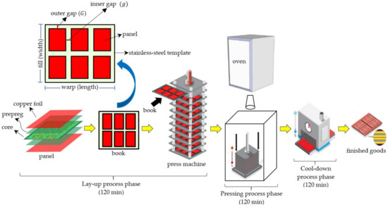 Figure 1. The overall processes of one cycle of a press machine.
- Lay-up process phase: The books are created and inserted into all openings (slots) of the press machine. The number of books that are inserted is equal to the number of openings of the press machine. This phase takes 120 min.
- Pressing process phase: The press machine, which is already inserted with books, is moved into an oven, and the books are pressed and heated in the oven. After 120 min, the press machine is removed from the oven.
- Cool-down process phase: The pressed books are cooled down for 120 min. Finally, the books are separated from the press machine to complete one press machine cycle.
- The three phases of the press machine cycle must be worked continually without idle time.
- A press machine can immediately start a new cycle after it has finished the previous cycle. Likewise, an oven is ready for the pressing process phase of another press machine after finishing the current pressing process phase.
- The company has a fixed number of press machines , each of which has openings, and a fixed number of ovens . Normally, a PCB company has a small number of ovens because the cost of an oven is very expensive.
- The company considers a planning horizon of 3 d. The maximum number of available cycles of each press machine to be operated in the pressing process is given. In reality, this value can be estimated from the order of the customers and the available resources by the production planning department.
In addition, this paper has the following two assumptions:
- The demands of panels from the customer can be satisfied within the planning horizon and available resources, i.e., the demands or inputs from the customer have a feasible schedule.
- The number of SSTs is unlimitedly available.
The three main constraints for the pressing process are as follows:
- The books that are pressed in all openings of a cycle of the press machine must have the same specifications, i.e., all books must have the same panel type, the same SST size, and the same layout. This constraint is needed to ensure that the pressure from the press machine will be equally distributed to each panel.
- An oven can perform the pressing process phase of only one press machine at a time.
- The number of outputs (finished goods) of each panel type must be greater than or equal to the demand.
The objective of the pressing process is to minimize the makespan. The minimum makespan implies a good utilization of available resources [23].
3. Improved MILP Model (Model 2)
This section presents Model 2 for pressing process scheduling. The parameters, sets, indices, and variables used in Model 2 are defined below.
Parameters:
- The number of panel types.
- The number of SST sizes.
- The number of layouts.
- The number of press machines.
- The number of ovens.
- The maximum number of available cycles of each press machine.
- The number of openings of each press machine.
- The processing time of each phase in the pressing process, i.e., the lay-up, pressing, and cool-down process phases. In our case, min.
- The number of panels of type per book (or per opening) using SST size and layout .
- The demand of panel type .
- A large positive number.
Sets:
- The set of all panel types, .
- The set of all SST sizes, .
- The set of all layouts, .
- The set of all press machines, .
- The set of all ovens, .
- The set of all numbers of available cycles of each press machine, .
Variables:
- 1, if panel type is assigned with SST size and layout to press machine at cycle , and 0 otherwise.
- 1, if press machine is sent into oven at cycle , and 0 otherwise.
- 1, if cycle of press machine is processed before cycle of press machine in the same oven, and 0 otherwise.
- The starting time of cycle of press machine (the starting time of the lay-up process phase).
- The starting time of the pressing process phase in cycle of press machine .
- The auxiliary variable which is equal to if there are a panel type, a SST size, and a layout assigned in press machine at cycle . Otherwise, it is equal to 0.
- The maximum completion time of the last cycle of all press machines that perform the pressing process (the makespan of the overall process).
Model 2 for scheduling the pressing process is as follows.
subject to:
and,
The objective function (1) is to minimize the makespan of the overall process.
Constraint (2) ensures that at most one type of panel, one size of SST, and one layout can be assigned in each cycle of each press machine. If there is an assignment of a panel type, a SST size, and a layout in a press machine cycle, it means that all books that are inserted in all openings of this press machine in this cycle are created using this pattern.
Constraint (3) makes sure that if panel type is not compatible with SST size and layout (), then this pattern cannot be assigned to any press machine cycle.
Constraint (4) enforces that the overall outputs of each panel type from all cycles of all press machines must satisfy the demand.
Constraint (5) ensures that a panel type, a SST size, and a layout must be assigned to consecutive cycles of a press machine. This helps push the empty cycles (the cycles of a press machine with no panel assignment) to be placed after the non-empty cycles (the cycles that really operate the pressing process).
Constraint (6) enforces that any press machine cycle must only be assigned to one oven.
Constraint (7) ensures that the starting time of a cycle of a press machine is not less than the completion time of the previous cycle. The completion time of the previous cycle is equal to its starting time plus the processing time (the processing time of one cycle). In other words, this constraint enforces that any cycle of a press machine can be started after the previous cycle has been completed.
Constraint (8) sets the starting time of the pressing process phase in cycle of press machine to be equal to the starting time of this press machine cycle plus the processing time that it takes in the lay-up process phase.
Constraints (9) and (10) make sure that the pressing process phase in cycle of press machine and the pressing process phase in cycle of press machine , which are assigned in the same oven , cannot be performed simultaneously. It depends on the binary variable . If , the pressing process phase in cycle of press machine precedes the pressing process phase in cycle of press machine in oven . Otherwise, the pressing process phase in cycle of press machine is performed after the pressing process phase in cycle of press machine in oven .
Constraints (11)–(13) enforce that if there is an assignment of a panel type, a SST size, and a layout in press machine at cycle , then the auxiliary variable is equal to . Otherwise, it is equal to 0. The auxiliary variable will be used in Constraint (14).
Lastly, Constraint (14) determines the maximum completion time of the last cycle of the press machines that really operate the pressing process or the makespan of the overall process.
Compared with Model 1 for scheduling the pressing process [10], Model 2, developed in this paper, has many improved parts as follows.
- The binary variable ( if press machine at cycle precedes press machine at cycle in oven ) in Model 1 is replaced by the new binary variable in Model 2, where both variables have the same role to avoid an overlapping of any two pressing process phases that are processed in the same oven . However, the definition of is without reference to the oven. This can significantly reduce the NBV in the model. Model 2 can still retrieve the oven information from the variables and . For example, assume that the variables . This means that press machine 1 at cycle 1 and press machine 2 at cycle 2 are assigned to do the pressing process phase in oven 1. Suppose that in Model 1 while in Model 2. The variable in Model 1 means that press machine 1 at cycle 1 is processed before press machine 2 at cycle 2 in oven 1, while the variable in Model 2 means that press machine 1 at cycle 1 is processed before press machine 2 at cycle 2 in the same oven. Although the variable in Model 2 does not give the oven information, it can be known from the variables , i.e., both tasks are processed in the same oven 1.
- The continuous variable , the starting time of the pressing process phase in cycle of press machine in oven , in Model 1 is replaced in Model 2 by the variable , which is without reference to the oven. This replacement can significantly reduce the NCV and eliminate some constraints in Model 1 that were related to the variable . For example, suppose that , which means that press machine at cycle is assigned to oven In Model 1, the constraint that forces the variable to be 0 is needed when press machine at cycle must not be assigned to oven so that the model has only the non-zero value of . In Model 2, however, this constraint is not needed because the model defines the variable , which has no oven index. If needed, Model 2 can retrieve the oven information from the variable to find which oven is assigned to press machine at cycle to do the pressing process phase. For example, assume that the variable , which means that press machine 2 at cycle 2 is assigned to do the pressing process phase in oven 1. Suppose that the variable min in Model 1 while the variable min in Model 2. The variable in Model 1 means that press machine 2 at cycle 2 starts the pressing process phase in oven 1 at time 480 while the variable in Model 2 means that press machine 2 at cycle 2 starts the pressing process phase at time 480. Although the variable in Model 2 does not give the oven information, it can be known from the variables , i.e., the press machine 2 at cycle 2 starts the pressing process phase at time 480 in oven 1.
- Model 2 does not use the variables about the completion times. In Model 1, the variables and , the completion time of cycle of press machine and the completion time of the pressing process phase in cycle of press machine in oven , respectively, were used. Model 2 can retrieve these values after solving the model where the former is equal to and the latter is equal to (the completion time is equal to the starting time plus the processing time). This can significantly reduce not only the NCV but also the NC in the model because the constraints that are related to the completion time variables are no longer needed.
- Model 1 used too many constraints to handle the non-overlapping conditions in the oven. It formulated the constraint in cases to avoid an overlapping of any two pressing process phases in the same oven. However, Model 2 formulates the constraint only in cases , which can completely define the non-overlapping conditions in the oven. This is because either Constraint (9) or Constraint (10) is active for any two pressing process phases from cycle of press machine and cycle of press machine , which are processed in the same oven . Constraint (9) is active if the task from cycle of press machine is processed before the task from cycle of press machine . Otherwise, Constraint (10) is active if the task from cycle of press machine is processed before the task from cycle of press machine . From the cases , it can guarantee that any two pressing process phases from any cycle of two press machines and , which are processed in the same oven, cannot overlap. It is clear that the non-overlapping conditions in the oven are completely defined, and the constraint in cases need not be considered.
4. Numerical Results
To evaluate the proposed MILP model, the previous data and test problems [10] were used. Furthermore, additional larger-sized (than in [10]) test problems were also generated in this paper. All problems were solved using both the previous Model 1 [10] and the proposed Model 2, and the results from both models were compared. The data and test problems are shown in Section 4.1, and the results from both models are shown in Section 4.2.
4.1. Data and Test Problems
The same data previously used for Model 1 [10], which were acquired from an actual PCB company, were used in this study and consisted of the following. The number of panel types , the number of SST sizes , the number of layouts , the number of press machines , and the number of ovens were seven, six, eight, six, and three, respectively. The number of openings of each press machine was 10. The sizes of each panel type, which included the warp and fill as well as the inner gap and outer gap , are shown in Table 3. The sizes of each SST, which included the warp and fill are shown in Table 4. Figure 2 shows the illustration of eight layouts [10]. Note that Figure 2 illustrates only examples that show the direction of the arrangement of panels on a SST. The number of panels in the book is not restricted to those shown in the illustration. For example, Figure 2a illustrates the first layout with two horizontal sections, and the panels are arranged vertically in each section. The company had the formulas for computing the number of panels of type per book based on SST size and layout , which are shown in Table 5. It should be noted that the notation is the largest integer that is less than or equal to . The processing time of each phase in the pressing process was assumed to be 120 min. In addition, the maximum number of available cycles of each press machine was 12. This is because the processing time of one cycle of a press machine is 360 min (6 h). If a press machine operates continually, it can conduct up to 12 cycles of the pressing process in 3 d.
Table 3.
Sizes, inner gap, and outer gap of each panel type.
Table 4.
Sizes of each SST.
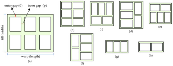
Figure 2.
Illustration of the eight layouts (a–h) of the panel arrangement [10].
Table 5.
Formulas for computing , which is the number of panels of type per book using SST size , and layout .
Moreover, the planning horizons of 2 and 1.5 d were also considered in [10] for different problem sizes, where the maximum number of available cycles of each press machine was eight and six, respectively. The previous test problems [10] were generated using the acquired data, and the parameters and in some test problems were also slightly different from the real data for a variety of the problem sizes. The demand of each panel type in each problem was randomly generated. The test problems were categorized into the three types of small, medium, and large problems, according to the NBV, and were totaled five, eight, and nine problems, respectively, as shown in Table 6, Table 7 and Table 8. A problem that has three panel types means that there are panel types 1–3 (in Table 3). Similarly, a problem that has four, five, six, or seven panel types means that there are panel types 1–4, 1–5, 1–6, or 1–7 (in Table 3), respectively.
Table 6.
The small problems.
Table 7.
The medium problems.
Table 8.
The large problems.
Furthermore, in this paper, additional test problems were generated using the data in [10]. The planning horizon of these problems was 4 d, where the maximum number of available cycles of each press machine was 16. The demand of each panel type in each problem was randomly generated. The additional test problems are shown in Table 9. Similarly, a problem that has five, six, or seven panel types means that there are panel types 1–5, 1–6, or 1–7 (in Table 3), respectively.
Table 9.
The additional test problems.
4.2. Computational Results
To compare the performance between Model 1 and Model 2, the two widely used performance measures of size and computational complexities were used. All problems were solved using ILOG OPL CPLEX 12.6 software running on a personal computer with a core i7 2.20 GHz CPU and 8 GB RAM, within a maximum time limit of 2 h.
4.2.1. Computational Results of the Small Problems
The model size, which included the NBV, the NCV, and the NC as well as the computational results of each small problem using Model 1 and Model 2, are shown in Table 10. The results included the number of outputs (finished goods) of each panel type, CPU time, and the makespan of the overall process. The last column in Table 10 reports the RPItime or the relative percentage improvement of the CPU times of Model 2 over Model 1, which is defined as .
Table 10.
Computational results of the small problems using Model 1 and Model 2.
As shown in Table 10, the NBV, NCV, and NC in Model 2 from each small problem were lower than those in Model 1. Figure 3a–c shows the NBV, NCV, and NC, respectively, for each model generated in each small problem. This reveals that Model 2 outperformed Model 1 in terms of the size complexity for the small problems. Both Model 1 and Model 2 could solve all the small problems to an optimal solution. The optimal makespan could be found, and the demand of each panel type was satisfied. For example, the optimal makespan of Problem S1 was 1,440 min, and the outputs of panel types 1–3 were 120, 160, and 160, respectively, which is greater than or equal to the demands of Problem S1 shown in Table 6. However, Model 2 could find an optimal solution for all small problems at a smaller CPU time. Figure 3d demonstrates the CPU time for solving each small problem using Model 1 and Model 2, where Model 2 also outperformed Model 1 in terms of the computational complexity for the small problems. From the last row of Table 10, Model 2 provided a better CPU time with an average RPItime of 36.84% for the small problems.
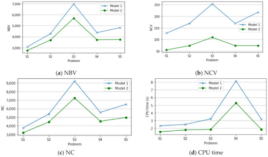
Figure 3.
Comparison of model sizes, as the (a) NBV (number of binary variables), (b) NCV (number of continuous variables), and (c) NC (number of constraints) and (d) the CPU times for solving the small problems between Model 1 and Model 2.
4.2.2. Computational Results of the Medium Problems
Table 11 shows the NBV, NCV, NC, and the results of each medium problem using Model 1 and Model 2. The number of NBV, NCV, and NC that Model 2 generated in each medium problem was less than those that Model 1 generated. Figure 4a–c shows the NBV, NCV, and NC, respectively, that each model generated for each medium problem, where Model 2 outperformed Model 1 in terms of the size complexity for the medium problems. Both models could find an optimal solution for all medium problems, but Model 2 could find the optimal solution using a smaller CPU time in all problems with an average RPItime of 69.98%. The CPU times used for solving each medium problem using Model 1 and Model 2 are shown in Figure 4d, where Model 2 also outperformed Model 1 in terms of the computational complexity for the medium problems.
Table 11.
Computational results of the medium problems using Model 1 and Model 2.
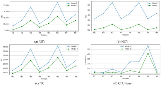
Figure 4.
Comparison of the model size, as the (a) NBV (number of binary variables), (b) NCV (number of continuous variables), and (c) NC (number of constraints) and (d) the CPU times for solving the medium problems between Model 1 and Model 2.
4.2.3. Computational Results of the Large Problems
Table 12 shows the NBV, NCV, NC, and the results for each large problem using Model 1 and Model 2. The results included the outputs, CPU time, %gap, and makespan . In Table 12, the column “CPU time” denotes the computational time taken by CPLEX to solve the MILP model to reach optimality, or 2 h if CPLEX cannot solve the MILP model optimally within the time limit. The %gap is the relative gap tolerance of the objective value for the solution from CPLEX, which is defined as . The is the current best feasible solution (or incumbent solution) that could be found by the model within the time limit, and the is the current lower bound that the model could obtain within the time limit. The smaller the %gap value is, the better performance the model will be. If the problem could be solved to reach optimality, then the %gap is equal to 0%. Note that, for the solution that we get within the time limit and %gap0, it needs to use more computational time than 2 h for solving the problem to reach optimality. The column “” reports the optimal makespan or the incumbent makespan that could be found within the time limit. Table 12 also reports timeinc, which is the computational time to reach the incumbent solution. For the problem that could be solved optimally, the timeinc is the time to reach the incumbent solution, which is an optimal solution, but the status of the problem at that time is not at optimality because the %gap is not equal to 0 at that time. The last column in Table 12 reports RPItime and , where the is the relative percentage improvement of timeinc of Model 2 over Model 1, and is defined as .
Table 12.
Computational results of the large problems using Model 1 and Model 2.
As shown in Table 12, the NBV, NCV, and NC in Model 2 for each large problem were lower than those in Model 1. Figure 5a–c shows the NBV, NCV, and NC, respectively, that each model generated in each large problem. Model 2 clearly outperformed Model 1 in terms of the size complexity for the large problems. Compared to Figure 3a–c and Figure 4a–c, the differences in the NBV and NC between the two models become more significant when the problem size increased from small to large.
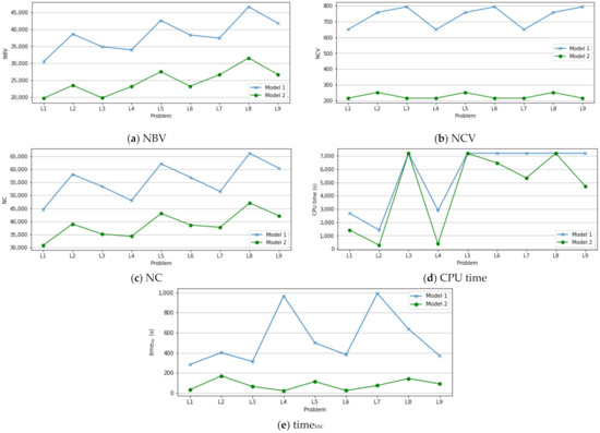
Figure 5.
Comparison of the model size, as the (a) NBV (number of binary variables), (b) NCV (number of continuous variables), and (c) NC (number of constraints) and the (d) CPU time and (e) timeinc (computational time to reach the incumbent solution) for solving the large problems between Model 1 and Model 2.
Furthermore, from Table 12, Model 1 could solve only three large problems optimally within the time limit (Problem L1, L2, and L4), whereas Model 2 could optimally solve these problems using a smaller CPU time. For Problem L6, L7, and L9, Model 1 could not solve them to reach optimality within the time limit since the %gap was not equal to 0%. However, Model 2 could solve these problems to reach optimality within the time limit (%gap = 0%). For Problem L3, L5, and L8, neither models could solve them to reach optimality. The makespan of the incumbent solution from Model 2 was equal to that from Model 1 (the incumbent solutions from both models have the same quality), and the values of %gap from both models were also the same in each problem. However, Model 2 used a smaller timeinc than Model 1 to reach the incumbent solution for these problems.
Figure 5d,e shows the CPU time and timeinc, respectively, for solving each large problem using Model 1 and Model 2. From Figure 5d, solving Problem L3, L5, and L8 using Model 1 and Model 2 was not achieved within the 2-h time limit, but a significant difference in the CPU times between the two models was evident for the other problems. From Figure 5e, moreover, Model 2 used a smaller timeinc to reach the incumbent solution for all the large problems. The average RPItime and values were 31.60% and 82.06%, respectively. These show that Model 2 outperformed Model 1 in terms of computational complexity for the large problems.
In a real-life application, any PCB manufacturing company may not need to solve a problem to reach optimality if it takes a long computational time, but the company needs to find a promising solution for the problem as fast as possible. The timeinc of each large problem using Model 2 was small and acceptable in a real-life application. The maximum value of timeinc to reach the incumbent for large problems using Model 2 is only 2 min 50 s (in Problem L2). Hence, Model 2 can fulfill this preference and can be a practical option to provide a promising schedule for the pressing process in any PCB manufacturing industry.
4.2.4. Computational Results of the Additional Test Problems
Table 13 shows the NBV, NCV, NC, and the results for each additional test problem using Model 1 and Model 2. Model 2 had lower NBV, NCV, and NC in each problem than Model 1. Figure 6a–c shows the NBV, NCV, and NC, respectively, that each model generated in each additional test problem. This revealed that Model 2 clearly outperformed Model 1 in terms of size complexity for the additional test problems.
Table 13.
Computational results of the additional test problems using Model 1 and Model 2.
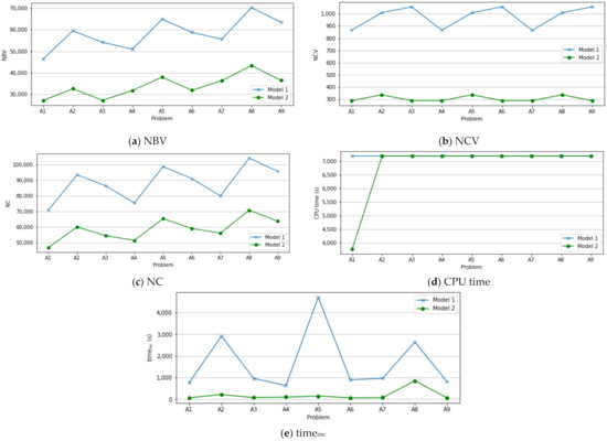
Figure 6.
Comparison of the model size, as the (a) NBV (number of binary variables), (b) NCV (number of continuous variables), and (c) NC (number of constraints) and the (d) CPU time and (e) timeinc (computational time to reach the incumbent solution) for solving the additional test problems between Model 1 and Model 2.
In addition, from Table 13, neither models could solve all the additional test problems optimally within the 2-h time limit, except for Model 2, which could solve Problem A1 optimally. For the problems that could not be solved optimally, both models could find the incumbent solution with the same value of makespan and %gap, except for Problem A2 and A8. For Problem A2, each model could find the incumbent solution with the same value of makespan, but the %gap from Model 2 (4.39%) was smaller than that from Model 1 (5.26%). In Problem A8, Model 2 could find a better incumbent solution ( = 4440 min) than that by Model 1 ( = 4560 min). For Problem A3–A7 and A9, the incumbent solutions from both models have the same quality, but Model 2 used less timeinc than Model 1 to reach the incumbent solution for these problems.
Figure 6d demonstrates the CPU time for solving each additional test problem using Model 1 and Model 2. The CPU time for solving Problem A1 using Model 2 was smaller than that using Model 1, but the CPU times for solving the other problems using both models were 2 h because they could not verify optimality within the time limit. However, Model 2 used a smaller timeinc to reach the incumbent solution for all additional test problems (Figure 6e). Thus, Model 2 saved a large amount of computational time to reach the incumbent solution, compared with Model 1, for all problems, where the quality of the incumbent solution from Model 2 was no worse than that from Model 1. For example, in Problem A8, Model 2 used a timeinc of 14 min 16 s to reach the incumbent solution ( = 4440 min) compared to 44 min 4 s ( = 4560 min) for Model 1. The timeinc used in the other problems using Model 2 varied in the range of only 1–4 min. The difference in timeinc between Model 1 and Model 2 is particularly prominent in Problem A2 and A5. Model 2 used a timeinc of only 3 min 43 s and 2 min 32 s to reach the incumbent solution of Problem A2 and A5, respectively, compared to 48 min 35 s and 78 min 26 s, respectively, for Model 1 with the same makespan. In addition, the average RPItime and were 5.28% and 88.70%, respectively. These show that Model 2 is very efficient and effective at finding a good solution within a small computational time and so can be a practical option in the real PCB manufacturing industry.
Moreover, the results from Model 2 can give useful information. For example, from Problem A1–A3 in Table 9, all the parameters in the problems were the same except for the number of press machines and ovens, where the number of press machines and ovens were increased (from Problem A1) by one in Problem A2 and A3, respectively. The results of these problems (Table 13) showed that the makespan of Problem A1–A3 were 5160 min, 4560 min, and 5160 min, respectively. This means that increasing the number of press machines by one from Problem A1 could reduce the makespan from 5160 to 4560 min, but increasing the number of ovens by one from Problem A1 could not reduce the makespan. Thus, Model 2 can help in deciding which resources should be increased to reduce the production time.
5. Discussions
Model 2 was found to outperform Model 1 in terms of all three structural elements of size complexity (the NBV, NCV, and NC). This is because Model 2 used the binary variable and the continuous variable instead of and in Model 1, respectively, which can reduce the NBV and NCV in the model, but the meaning of both models remained the same. It can also reduce the NC that are related to the index of the oven. In addition, the dimensionalities of the two decision variables were also reduced because the variables and have five and three indices, but the variables and have only four and two indices, respectively. Moreover, Model 2 did not use the variables that were related to the completion time and could reduce the NC to handle the non-overlapping conditions in an oven. Some examples of these replacements and eliminations are provided in Section 3. Since the most deciding factor that affects the performance of a MILP is the NBV, and the next influential factor is the NC [11], reducing these in Model 2 can help to solve large-sized problems more efficiently.
Furthermore, Model 2 used less computational time than Model 1 for solving all the problems that could be solved to reach optimality. It could also newly verify an optimal solution for some large problems and additional test problems that Model 1 could not. The average RPItime of the small, medium, large, and additional test problems were 36.84%, 69.98%, 31.60%, and 5.28%, respectively, where the average RPItime of all problems is 34.71%. In addition, Model 2 used a smaller computational time to find the incumbent solution for all the problems that could not be solved optimally within the 2-h time limit, where the incumbent solution from Model 2 is better or has the same quality as the incumbent solution from Model 1. The average of the large and additional test problems were 82.06% and 88.70%, respectively. Thus, Model 2 also outperformed Model 1 in terms of computational complexity. Note that, although the average RPItime of the additional test problems is small, because most of them could not be solved optimally, the average is still very high. This shows that Model 2 is very effective at finding the incumbent solution for large-sized problems within a relatively short time.
The computational times of Model 2 to reach the incumbent solution of large problems with a planning horizon of 3 d and additional test problems with a planning horizon of 4 d are small and practicable. In the real situation, a PCB company needs to find a good schedule for the pressing process scheduling within a small computational time, and an incumbent solution can be just what they need. Hence, in practice, a PCB company can use Model 2 to find an optimal solution or a good feasible solution for pressing process scheduling by setting a small time limit, such as 5 min, or by setting a small %gap, such as 5%.
Moreover, the proposed Model 2 has implications for both theory and practice. In theory, the techniques to reduce the model size in this paper can be applied to other similar scheduling problems. In practice, the following are examples of the real-world situations that can be beneficial from Model 2.
- A PCB company which manually schedules the pressing process can use the proposed model to find an optimal schedule or a good feasible schedule for the pressing process scheduling. The manager of the PCB company can compare the solution from the proposed model with the manual schedule and choose the better schedule to proceed in the real situation.
- In case of a rush order, a PCB company can use the proposed model to decide which resources should be increased to reduce the production time before proceeding in the real situation. For example, the manager of the PCB company can try to increase the parameters in the proposed model (e.g., the number of press machines or the number of ovens) and find how much the makespan can be reduced.
6. Conclusions
This study investigated pressing process scheduling, which is a real-world application in the PCB manufacturing industry. An application of MILP for pressing process scheduling is presented. The objective of the problem was to minimize the makespan. This objective can imply maximizing the utilization of the resources, which is usually the main objective of any PCB manufacturing enterprise.
The aim of this study was to improve the existing MILP model (Model 1 [10]) for solving pressing process scheduling. The obtained improvement (Model 2) revealed the possible application of MILP to handle an application in the real-world industry. The development of MILP models is interesting because the MILP model has the benefit that it can guarantee an optimal solution if one exists. MILP is also an approach that is widely used to cope with problems coming from organizations or industries. In this study, the previous Model 1 [10] and the improved Model 2 of this study were used to solve problems in the literature and additional test problems that were newly generated, and then, the computational results from both models were compared. The models were compared in terms of both size and computational complexities. The results show that Model 2 outperformed Model 1 in terms of both complexities. For the problems that could be solved optimally by Model 1, Model 2 could also solve them optimally but using less computational time. Furthermore, Model 2 could newly verify the optimal solution for some large problems and some additional test problems within the 2-h time limit. Model 2 also used an acceptable computational time (and less than Model 1) to find the incumbent solution for all the problems that could not be solved to reach optimality, where the makespan of the incumbent solution from Model 2 was less than or equal to the makespan of that from Model 1. In actual practice, a PCB company needs to use a small computational time to provide an effective schedule for the problem at hand. Therefore, Model 2 is suitable to use in actual practice.
The limitation of this approach is that the MILP model is not effective for solving pressing process scheduling problems with large planning horizons, such as, a period of a month. This is because the size of the model will become very large, which leads to a very long computational time. To be practical, it needs to use other methods, such as heuristic and metaheuristic algorithms, for solving long-term pressing process scheduling.
For future research, some extensions of the MILP model for the pressing process with additional constraints could be of interest. For example, the panel types have different cycle times and different due dates, one cycle of a press machine can press a group of compatible panel types, and press machines or ovens require machine maintenance. These additional constraints increase the complication of the problem, but it can be very challenging for further research. Another future research line is to develop heuristic or metaheuristic algorithms for solving pressing process scheduling problems using the solutions from the MILP model in this paper as references.
Author Contributions
Conceptualization, T.L., B.I., and C.J.; methodology, T.L., B.I., and C.J.; software, T.L.; validation, T.L., B.I., and C.J.; formal analysis, T.L., B.I., and C.J.; investigation, T.L., B.I., and C.J.; resources, C.J.; data curation, C.J.; writing—original draft preparation, T.L.; writing—review and editing, B.I. and C.J.; visualization, T.L.; supervision, B.I. and C.J. All authors have read and agreed to the published version of the manuscript.
Funding
This research received no external funding.
Acknowledgments
This work was supported in part by the Development and Promotion of Science and Technology Talented Project (DPST), Thailand, in part by the Center of Excellence in Logistics and Supply Chain Systems Engineering and Technology (LogEn Tech), Sirindhorn International Institute of Technology, Thammasat University, Thailand, and in part by Department of Mathematics and Computer Science, Faculty of Science, Chulalongkorn University, Thailand.
Conflicts of Interest
The authors declare no conflict of interest.
References
- Noroozi, A.; Mokhtari, H. Scheduling of printed circuit board (PCB) assembly systems with heterogeneous processors using simulation-based intelligent optimization methods. Neural. Comput. Appl. 2015, 26, 857–873. [Google Scholar] [CrossRef]
- Qin, W.; Zhuang, Z.; Liu, Y.; Tang, O. A two-stage ant colony algorithm for hybrid flow shop scheduling with lot sizing and calendar constraints in printed circuit board assembly. Comput. Ind. Eng. 2019, 138, 106115. [Google Scholar] [CrossRef]
- Khandpur, R.S. Printed Circuit Boards: Design, Fabrication, Assembly and Testing; McGraw-Hill: New York, NY, USA, 2006. [Google Scholar]
- Pezzella, F.; Morganti, G.; Ciaschetti, G. A genetic algorithm for the flexible job-shop scheduling problem. Comput. Oper. Res. 2008, 35, 3202–3212. [Google Scholar] [CrossRef]
- Ozguven, C.; Ozbakir, L.; Yavuz, Y. Mathematical models for job-shop scheduling problems with routing and process plan flexibility. Appl. Math. Model. 2010, 34, 1539–1548. [Google Scholar] [CrossRef]
- Demir, Y.; Isleyen, S.K. Evaluation of mathematical models for flexible job-shop scheduling problems. Appl. Math. Model. 2013, 37, 977–988. [Google Scholar] [CrossRef]
- Roshanaei, V.; Azab, A.; ElMaraghy, H. Mathematical modelling and a meta-heuristic for flexible job shop scheduling. Int. J. Prod. Res. 2013, 51, 6247–6274. [Google Scholar] [CrossRef]
- Naderi, B.; Gohari, S.; Yazdani, M. Hybrid flexible flowshop problems: Models and solution methods. Appl. Math. Model. 2014, 38, 5767–5780. [Google Scholar] [CrossRef]
- Meng, L.; Zhang, C.; Shao, X.; Zhang, B.; Ren, Y.; Lin, W. More MILP models for hybrid flow shop scheduling problem and its extended problems. Int. J. Prod. Res. 2020, 58, 3905–3930. [Google Scholar] [CrossRef]
- Laisupannawong, T.; Intiyot, B.; Jeenanunta, C. Mixed-integer linear programming model and heuristic for short-term scheduling of pressing process in multi-layer printed circuit board manufacturing. Mathematics 2021, 9, 653. [Google Scholar] [CrossRef]
- Pan, C.H. A study of integer programming formulations for scheduling problems. Int. J. Syst. Sci. 1997, 28, 33–41. [Google Scholar] [CrossRef]
- Unlu, Y.; Mason, S.J. Evaluation of mixed integer programming formulations for non-preemptive parallel machine scheduling problems. Comput. Ind. Eng. 2010, 58, 785–800. [Google Scholar] [CrossRef]
- Naderi, B.; Azab, A. An improved model and novel simulated annealing for distributed job shop problems. Int. J. Adv. Manuf. Technol. 2015, 81, 693–703. [Google Scholar] [CrossRef]
- Chen, J.S.; Yang, J.S. Model formulations for the machine scheduling problem with limited waiting time constraints. J. Inf. Optim. Sci. 2006, 27, 225–240. [Google Scholar] [CrossRef]
- Naderi, B.; Fatemi Ghomi, S.M.T.; Aminnayeri, M.; Zandieh, M. A study on open shop scheduling to minimise total tardiness. Int. J. Prod. Res. 2011, 49, 4657–4678. [Google Scholar] [CrossRef]
- Mousakhani, M. Sequence-dependent setup time flexible job shop scheduling problem to minimise total tardiness. Int. J. Prod. Res. 2013, 51, 3476–3487. [Google Scholar] [CrossRef]
- Mehrabad, M.S.; Fattahi, P. Flexible job shop scheduling with tabu search algorithms. Int. J. Adv. Manuf. Technol. 2007, 32, 563–570. [Google Scholar] [CrossRef]
- Fattahi, P.; Mehrabad, M.S.; Jolai, F. Mathematical modeling and heuristic approaches to flexible job shop scheduling problems. J. Intell. Manuf. 2007, 18, 331–342. [Google Scholar] [CrossRef]
- Roshanaei, V.; ElMaraghy, H.; Azab, A. Sequence-based MILP modeling for flexible job shop scheduling. In Proceedings of the IIE Conference & Expo 2012, Orlando, FL, USA, 19–23 May 2012. [Google Scholar]
- Naderi, B.; Azab, A. Modeling and heuristics for scheduling of distributed job shops. Exp. Syst. Appl. 2014, 41, 7754–7763. [Google Scholar] [CrossRef]
- Wang, F.; Tang, Q.H.; Rao, Y.Q.; Zhang, C.Y.; Zhang, L.P. Efficient Estimation of Distribution for Flexible Hybrid Flow Shop Scheduling. Acta. Autom. Sin. 2017, 43, 280–292. [Google Scholar]
- Meng, L.; Zhang, C.; Ren, Y.; Zhang, B.; Lv, C. Mixed-integer linear programming and constraint programming formulations for solving distributed flexible job shop scheduling problem. Comput. Ind. Eng. 2020, 142, 106347. [Google Scholar] [CrossRef]
- Pinedo, M.L. Scheduling: Theory, Algorithms, and Systems, 3rd ed.; Springer: New York, NY, USA, 2008. [Google Scholar]
Publisher’s Note: MDPI stays neutral with regard to jurisdictional claims in published maps and institutional affiliations. |
© 2021 by the authors. Licensee MDPI, Basel, Switzerland. This article is an open access article distributed under the terms and conditions of the Creative Commons Attribution (CC BY) license (https://creativecommons.org/licenses/by/4.0/).