Synchronization of a Network Composed of Stochastic Hindmarsh–Rose Neurons

Abstract

An algorithm for synchronization of a network composed of interconnected Hindmarsh–Rose neurons is presented. Delays are present in the interconnections of the neurons. Noise is added to the controlled input of the neurons. The synchronization algorithm is designed using convex optimization and is formulated by means of linear matrix inequalities via the stochastic version of the Razumikhin functional. The recovery and the adaptation variables are also synchronized; this is demonstrated with the help of the minimum-phase property of the Hindmarsh–Rose neuron. The results are illustrated by an example.

1. Introduction

1.1. Synchronization of Complex Networks and Multi-Agent Systems

Many natural and man-made systems can be described by means of the complex networks, e.g., communication networks, social networks, metabolic networks, neural networks, collaboration networks, economic networks, food webs, electric power grids among others, etc. This is why complex networks (CN) and multi-agent systems have been intensively investigated during the recent times. The tool to study these networks is the classical graph theory and, in some cases, the random graph theory as presented e.g., in [1]. The common feature of these systems is that they admit a representation by a graph consisting of nodes (agents, vertices) interconnected by the links (edges) in a certain topology—such a structure is called a complex network or a multi-agent system. One could observe a rapidly raising interest in the study of the synchronization between nodes of complex networks or, alternatively, synchronization (concensus) of agents in a multi-agent system. Synchronization is one of the simplest types of collective dynamics of the interconnected systems, but there is a significant phenomenon in the nature and it is often understood as a collective state of coupled systems [2]. There are many types of synchronization: One of the widely studied types of the synchronization is the identical (complete) synchronization (IS). Here, the states of the coupled systems should mutually converge to each other. IS of the coupled systems was initiated by [3,4] while Ref. [5] started analysis of the synchronization phenomena between interconnected chaotic systems. Except for the identical synchronization, the number of other kinds of synchronization of coupled systems were introduced, such as phase synchronization (PS) [6], generalized synchronization (GS) [7,8], projective synchronization [9], lag synchronization (LS) [10], $\epsilon$-synchronization [11], etc. GS implies a synchronization between nonidentical systems or identical systems with different parameters. The main synchronization condition in GS is the existence of the functional relationship between interconnected systems. The mutual false neighbor’s method for detection of the GS was proposed in [7]. Another method of the detection of the generalized synchronization is the auxiliary system approach [12]. This method is effective for the detection of the GS regime in the oriented CN with ring topology [13]. Another method, the so-called duplicated system approach, used for the detection of the GS regime in the CN, was introduced in [14]. The appropriate conditions of the GS of interconnected chaotic systems have widely studied in the last decade [15,16,17,18,19,20]. Note that numerical methods used for the numerical implementation of the dynamic of interconnected chaotic systems can affect the process of their synchronization [21,22,23,24].

It is noteworthy that not only the structure of the network but also the presence of different types of disturbances in the communication channels, e.g., the limited-band data erase [25], time delays [16,26,27], noise [16,28], quantization [29], etc., is a crucial feature having influence on the quality and the speed of the synchronization of the coupled systems [2,30,31]. The control of the complex networks and the multi-agent systems is often subjected to time delays. Synchronization of the CN under the time delays has been investigated in [26]. The situation is more complicated in the case of the heterogeneous time delays [32,33]. As shown in [26], an error can appear. Its norm does not converge to zero then. It is advantageous that many of the control designs solving the synchronization problem lead to the problem of a solution of a set of linear matrix inequalities (LMI) which is a convex optimization problem that can be efficiently solved.

If the transmission of information is conducted through the noisy channels, the received information is deformed by a random part. Hence, the control must be designed so that it is capable of minimizing damage caused by this perturbation. Multi-agent systems with noise are investigated in [34], where the LMI-based control design for synchronization of such a system is derived. Ref. [35] presents a design of a synchronization control for a stochastic system with uncertainties and jumping controls. Last but not the least, let us mention a survey [36] where the reader can find information about further works dealing with this field.

Note that different types of topology of complex networks have been studied. The topology defines the structural characteristics of the complex networks: how all nodes are interconnected with each other. For example, in the case of computer networks, there are several types of topologies like tree, star, ring, line (bus, chain), mesh, or a combination of them. One of the conditions of the synchronization of the nodes in the directed complex networks or agents in multi-agent systems is the appropriate topology of the directed complex network or multi-agent system. As noted in [37], the topology of the synchronizable network is a directed graph that contains a rooted directed spanning tree, where master (leader) is a root. On the other hand, the directed complex network with ring topology is always synchronizable [37]. In the case of the tree, star, line (bus, chain) topology, the master (leader) node influences directly or indirectly all other nodes in the complex network. This phenomenon is well-known and is used for the master–slave synchronization in the complex networks or leader-following consensus in the multi-agent systems. If the complex network is described by a ring topology, the result of the synchronization is not so trivial because each node of the network is connected with another node of the network. In Section 7, there is an example of the multi-agent system containing the leader node influencing five nodes interconnected in a circle. All of the nodes, except for the leader one, are influenced directly or indirectly by another nodes of network, and this topology is not so trivial in comparison with the tree or chain topology.

1.2. Synchronization of Neurons

It is a commonly recognized fact that a wide range of types of the complex behavior depending on external input (represented by the external current of ions) can be observed in neurons. This dependence is described e.g., in [38,39]: if the influx current is small enough, the neuron can rest in a quiescent state. After the increasing of this current, the neuron exhibits the periodic spikes, one spike per period. A further increase of the current leads to a number of spikes during one period. If this current is increased more, the chaotic behavior takes place. Thus far, a complete understanding of these phenomena has not been achieved. However, it is an intensively studied research topic as it is vital not only for recognition of the causes and proposing of the treatment for various health problems, like epileptic attacks, Parkinson’s disease, etc., but it is also crucial for the obtaining of a thorough insight into the functioning of the entire neural system.

Several models were developed with the aim of providing help for us to understand the functions of a neuron. Let us mention the Hodgkin–Huxley model (HH) [40] first. The advantage of its model is in its accuracy in the describing of a neuron function, although it is rather complicated. In addition, the problem of the choosing of the numerical method for the numerical implementation of the dynamics of individual HH neurons is not a trivial task [41,42]. In contrast, the Fitzhugh–Nagumo (FN) [43,44] model of neuron features is more simple but illustrates some phenomena (e.g., bursting) less accurately. The Hindmarsh–Rose (HR) neuron [45] can be regarded as a compromise between the requirements for simplicity and accuracy. This is advantageous when modeling a network composed of HR neurons. A detailed description of bifurcations as well as oscillatory and chaotic phenomena occurring in the HR neuron can be found e.g., in [38,39]. Behavior of the stochastic HR neurons has been investigated in e.g., [46].

Ref. [47] deals with the synchronization of a neuronal network with a linear feedback while master–slave synchronization of a pair of HR neurons is studied in [48]. Nonlinear coupling functions for chaotic synchonization of HR neurons are applied in e.g., [49,50,51,52]. Enhancement of synchronization by using a memristor is studied in [53] while an algorithm for synchronization of a network composed of HR neurons is presented in [54]. The coupling of neurons by a magnetic flux is described in [55]. The phenomenon of partially spiking chimera behavior, induced in the complex networks of bistable neurons with excitatory coupling, is studied in [56]. The adaptive synchronization for fitting values of some parameters of the model is presented e.g., in [57], while a similar problem for general chaotic systems is studied in [58]. Let us mention that the firing pattern of the neurons is dependent on the interconnection topology of the neural network as pointed out e.g., in [59]. The synchronization of the heterogeneous FN neurons with delays is studied in [60,61]. This problem is closely related to the one solved in this paper.

All the mentioned papers were devoted to the synchronization of a network composed of identical neurons. Contrary to this, Ref. [11] deals with the synchronization of the heterogeneous networks of FN neurons while desynchronization of FN neurons is described in [62] or [63].

1.3. Purpose and Outline of This Paper

The synchronization of a network composed of HR neurons subjected to random disturbances and delayed communication using the exact feedback linearization is investigated in this paper. Since an exact feedback linearization-based algorithm for the synchronization of a nonlinear multi-agent systems was introduced for general systems in [64,65] with satisfactory results, the aim of this paper is to apply this method to the case of a neuronal network composed of HR neurons. Moreover, the effects of noise are investigated, which, together with presence of delays, lead to the need of the combining of the aforementioned method with the stochastic version of the Razumikhin functional. We believe this problem in the described settings has not been studied so far. Preliminary results without proofs and with less extensive simulations were presented in [66].

The paper is organized as follows: in the Section 2, the necessary notions from the graph theory are presented. Section 3 contains a brief description of a stochastic multi-agent systems. Then, the Hindmarsh–Rose neuronal model is presented in Section 4 together with a short description of its properties. Section 5 is devoted to the synchronization of the membrane potential while Section 6 contains the proof of synchronization of the recovery and adaptation variables. Section 7 contains an illustrative example. This section is followed by the conclusions.

1.4. Notation

The notation used in this paper is introduced here.

• The Kronecker product is denoted by the symbol ⊗.
• The expected value of a random variable $\phi$ is denoted by $\mathbb{E}\left(\phi \right)$.
• If $A,B$ are matrices, then $\mathrm{diag}(A,B)$ is a block-diagonal matrix with blocks $A,B$ on the diagonal.
• The symbol ${}^T$ denotes the transposed matrix.
• The time argument t is often omitted: $f\left(t\right)=f$. However, if dependence on this time argument needs to be emphasized or the time argument is different from t, it is written in full.
• The time delay is written in the subscript: $f(t-\tau \left(t\right))=f(t-\tau )=f_{\tau }\left(t\right)=f_{\tau }$.
• The N-dimensional identity matrix is denoted by I.

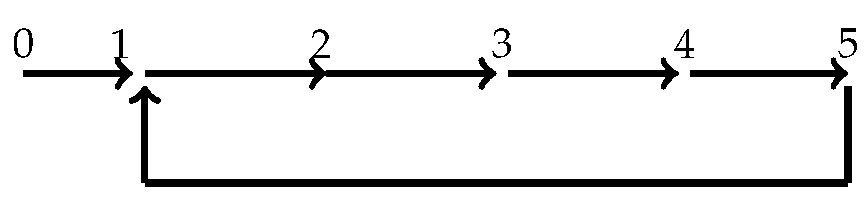
2. Graph Theory

The interconnection of the neurons in the network is described by means of the graph theory as follows: the neurons are assigned by numbers $0,\cdots ,N$. Define the set of nodes $\mathcal{V}=\{0,\cdots ,N\}$ and the set of edges $\mathcal{E}\subset \mathcal{V}\times \mathcal{V}$ as $(i,j)\in \mathcal{E}$ if there exists a connection from node i to node j: the neuron i can send a signal to neuron j directly. It is supposed that no neuron can send signals to itself: this implies $(i,i)\notin \mathcal{E}$ for any $i\in \mathcal{V}$.

Then, the graph describing the interconnection topology $\mathcal{G}$ is given as a pair $\mathcal{G}=(\mathcal{V},\mathcal{E})$. A very useful matrix for the future purpose is the Laplacian matrix $\mathcal{L}\in {\mathbb{R}}^{(N+1)\times (N+1)}$, defined for the graph $\mathcal{G}$ as follows: for $i,j\in \{0,\cdots ,N\}$, $i\ne j$, one defines ${\mathcal{L}}_{i,j}=-1$ if $(j,i)\in \mathcal{E}$; otherwise, ${\mathcal{L}}_{i,j}=0$. Moreover, the diagonal elements are defined as ${\mathcal{L}}_{i,i}=-{\sum }_{j=1,i\ne j}^N{\mathcal{L}}_{i,j}$. We also define the sets $N_i\subset \mathcal{V}$, $i=1,\cdots ,N$ as $N_i=\{j\in \mathcal{V}|(j,i)\in \mathcal{E}\}$. The set $N_i$ also contains all agents that send information directly to the agent i.

We assume the existence of one neuron $i_0$ such that, for any $j\in \mathcal{V}$, $i_0\ne j$ there exists a directed path in $\mathcal{G}$ from $i_0$ to j (that means, there exists a finite sequence $(i_0,i_1),(i_1,i_2),\cdots ,(i_{k-1},i_k)$ for some $k\in \mathbb{N}$ such that $i_k=j$ and for any $k^{\prime }\in \{1,\cdots ,k\}$ holds $i_{k^{\prime }}\in \mathcal{V}$, $(i_{k^{\prime }-1},i_{k^{\prime }})\in \mathcal{E}$), but there is no path from any $j\ne i_0$ to $i_0$. The node $i_0$ enjoying this property is called the leader. In our framework, it is a neuron whose behavior all other neurons replicate. Without loss of generality, we can assume $i_0=0$. (For more details and explanations, refer to [67]).

Let us also introduce matrix $L\in {\mathbb{R}}^{N\times N}$ by removing the first row and column (the row and column corresponding to the leader) from matrix $\mathcal{L}$. As demonstrated in [68,69], eigenvalues of matrix L have positive real parts and, moreover, there exists a diagonal matrix $D=\mathrm{diag}(d_1,\cdots ,d_N)$ with $d_i>0$ so that

$$DL+L^{T}D>0.$$

(1)

Denote $d_{max}=max\left\{d_i\right|i=1,\cdots ,N\}$. Finally, let us also define the pinning matrix $G\in {\mathbb{R}}^{N\times N}$ by $G=\mathrm{diag}(g_1,\cdots ,g_N)$, where $g_i=1$ if $(0,i)\in \mathcal{E}$; otherwise, $g_i=0$. This matrix describes how the information from the leader is pinned into the network of the other neurons. The structure of the interconnection of these neurons is described by the matrix $\overline{L}=L-G$.

3. Synchronization of Stochastic Multi-Agent Systems

The synchronization of linear multi-agent systems is thoroughly described e.g., in [34]. Therefore, only the most important facts are repeated here.

A stochastic multi-agent system can be described as a network composed of agents in a form

$$\begin{array}{cc}\hfill d{x}_0=& A{x}_0+{\widehat{\sigma }}_0\left(x_0\right)dw\left(t\right),\hfill \end{array}$$

(2)

$$\begin{array}{cc}\hfill d{x}_i=& (A{x}_i+B{u}_i)dt+{\widehat{\sigma }}_i\left(x_i\right)dw\left(t\right),i=1,\cdots ,N.\hfill \end{array}$$

(3)

Here, $x_i\in {\mathbb{R}}^n$ is the state of the ith agent, $u_i$ is its control, ${\widehat{\sigma }}_i:{\mathbb{R}}^n\to \mathbb{R}$ are the noise intensity functions, $w\left(t\right)$ is a one-dimensional Wiener process defined on $(\Omega ,\mathcal{F},\mathcal{P})$ such that $\mathbb{E}\left(w\right(t\left)\right)=0$, $\mathbb{E}\left({\left(w\left(t\right)\right)}^2\right)=dt$.

As noted in [34], this model is suitable to describe random external disturbances acting upon the whole multi-agent system. This is why it is used in this paper as well.

The goal is to find the control $u_i$ as a function of the state $x_i,x_j,j\in N_i$ so that

$$\underset{t\to \infty }{lim}\mathbb{E}(\parallel x_i\left(t\right)-x_0\left(t\right){\parallel }^2)=0.$$

(4)

4. The Hindmarsh–Rose Neuronal Model

According to e.g., [48], the HR neuron is defined by the following equations:

$$\begin{array}{cc}\hfill {\dot{x}}_1=& a{x}_1^2-x_1^3+x_2-x_3+I+\overline{\sigma }\left(x_1\right)dw\left(t\right),\hfill \end{array}$$

(5)

$$\begin{array}{cc}\hfill {\dot{x}}_2=& 1+b{x}_1^2-x_2,\hfill \end{array}$$

(6)

$$\begin{array}{cc}\hfill {\dot{x}}_3=& c(x_1+1.56)-0.006x_3.\hfill \end{array}$$

(7)

The variable $x_1$ is the membrane potential, $x_2$ denotes the recovery variable associated with the fast current of the Na${}^{+}$ and/or K${}^{+}$ ions, and $x_3$ stands for the adaptation variable associated with the slow current of Ca${}^{+}$ ions. Moreover, the symbol I denotes the external current. The random part, denoted by $\overline{\sigma }\left(x\right)$ here with $\overline{\sigma }:\mathbb{R}\to \mathbb{R}$, is described in the sequel. Finally, w is the noise satisfying properties presented in the previous section.

Values of the constants are presented in [48]; for the reader’s convenience, they are repeated here: $a=3$, $b=-5$, $c=0.024$ and $I=1.25$.

Remark 1.

The behavior of the HR neuron varies significantly in the dependence on the external current. For example, for the model given by (5)–(7), that periodic spiking can be observed for $I>3.25$, chaotic behavior is exhibited for $I\in (2.75,3.25)$, while, for $I<2.75$, the neuron is in the state of periodic bursting and, finally, the quiescent state appears for $I<1.14$. For details, see [48].

To apply the exact feedback linearization-based method presented in [65], we proceed on every neuron as follows. For every $i\in \{0,\cdots ,N\}$, define the output of the ith neuron as $y_i=x_{1,i}$ (the membrane potential). As will be seen in the subsequent text, this choice is suitable in the sequel since this is the coupling variable. The exact feedback linearization attains a rather simple form (with $j=1,2,3$):

$$\begin{array}{c}\hfill {\xi }_{1,i}=x_{1,i},{\xi }_{2,i}=x_{2,i},{\xi }_{3,i}=x_{3,i}\end{array}$$

(8)

$$\begin{array}{c}\hfill F\left({\xi }_i\right)=-a{\xi }_{1,i}^2-{\xi }_{1,i}^3+{\xi }_{2,i}-{\xi }_{3,i}+I,\end{array}$$

(9)

$$\begin{array}{c}\hfill u_i=v_i-F\left({\xi }_i\right),\end{array}$$

(10)

The system of Equations (5)–(7) is transformed into the following linear system (this transformation is a diffeomorphism as shown in [70]):

$${\dot{\xi }}_i=\left(\begin{array}{c}0\\ -{\xi }_{2,i}\\ -0.006{\xi }_{3,i}\end{array}\right)+\left(\begin{array}{c}{v}_i\\ 0\\ 0\end{array}\right)+\left(\begin{array}{c}0\\ 1\\ 1.56c\end{array}\right).$$

(11)

The variable ${\xi }_i=({\xi }_{1,i},{\xi }_{2,i},{\xi }_{3,i})$ is divided into two parts: ${\xi }_i={({\eta }_i,{\zeta }_i^T)}^T$ where ${\eta }_i={\xi }_{1,i}$, $\zeta ={({\xi }_{2,i},{\xi }_{3,i})}^T$. The first equation described by the variable ${\eta }_i$ will be called the observable part, and the remaining part is the non-observable part. This terminology is based on the fact that the state ${\zeta }_i$ is not observable through the output $y_i$ (however, note that, in order to control the system (5)–(7), access to the state ${\zeta }_i$ is necessary). Moreover, one can introduce the zero dynamics by

$${\dot{\zeta }}_i=\left(\begin{array}{c}-{\zeta }_{1,i}\\ -0.006{\zeta }_{2,i}\end{array}\right).$$

(12)

Obviously, from (12), one can see that the HR neuronal model exhibits an asymptotically stable zero dynamics.

Remark 2.

Note that, if a system has asymptotically stable zero dynamics, then it is called a minimum-phase system [70].

As will be seen from the subsequent text, this is a crucial property allowing for applying the synchronization algorithm described in [64].

Consider now the network composed of $N+1$ neurons denoted by $0,\cdots ,N$. It is assumed that the neuron with index 0 is the leader. If $i\in \{1,\cdots ,N\}$, then the ith neuron with coupling can be described as

$$\begin{array}{cc}\hfill {\dot{x}}_{1,i}=& a{x}_{1,i}^2-x_{1,i}^3+x_{2,i}-x_{3,i}+I+u_i+{\tilde{\sigma }}_i\left(x_{1,i}\right)dw\left(t\right),\hfill \end{array}$$

(13)

$$\begin{array}{cc}\hfill {\dot{x}}_{2,i}=& 1+b{x}_{1,i}^2-x_{2,i},\hfill \end{array}$$

(14)

$$\begin{array}{cc}\hfill {\dot{x}}_{3,i}=& c(x_{1,i}+1.56)-0.006x_{3,i}.\hfill \end{array}$$

(15)

Here, $u_i$ is the input signal which is to be designed in the subsequent text. This signal contains the coupling between different neurons.

For simplicity, we suppose that this delay, denoted by $\tau$, is equal for all neurons in the network; however, it is not required to be constant. To be precise, there exists a constant $\overline{\tau }>0$ so that $\tau :[0,\infty )\to [0,\overline{\tau }]$ is a measurable function. The control of the ith neuron, denoted by $u_i$, attains the form

$$u_i=-F\left(x_i\right)+k\left(\sum _{j\in N_i}(x_{1,j;\tau }-x_{1,i;\tau })+g_i(x_{1,0;\tau }-x_{1,i;\tau })\right),$$

(16)

where the gain k is called a coupling gain, the coupling is conducted through the term ${\sum }_{j\in N_i}(x_{1,j;\tau }-x_{1,i;\tau })+g_i(x_{1,0;\tau }-x_{1,i;\tau })$. It is assumed that the signals from the other neurons are arriving with delay. The goal is to determine constant k so that (4) is achieved. This constant is equal for the all of the neurons in the network.

Substituting (16) into (13) yields the description of the ith neuron ($i=1,\cdots ,N$):

$${\dot{x}}_{1,i}=a{x}_{1,i}^2-x_{1,i}^3+x_{2,i}-x_{3,i}+I+{\tilde{\sigma }}_i\left(x_{1,i}\right)dw\left(t\right)-F\left(x_i\right)+k(\sum _{j\in N_i}(x_{1,j;\tau }-x_{1,i;\tau })+g_i(x_{1,0;\tau }-x_{1,i;\tau })),$$

(17)

$$\begin{array}{cc}\hfill {\dot{x}}_{2,i}=& 1+b{x}_{1,i}^2-x_{2,i},\hfill \end{array}$$

(18)

$$\begin{array}{cc}\hfill {\dot{x}}_{3,i}=& c(x_{1,i}+1.56)-0.006x_{3,i}.\hfill \end{array}$$

(19)

Observe also that the control of the ith neuron after the transformation given by (10) is expressed by the formula

$$v_i=k\left(\sum _{j\in N_i}({\xi }_{1,j,\tau }-{\xi }_{1,i,\tau })+g_i({\xi }_{1,0,\tau }-{\xi }_{1,i,\tau })\right).$$

(20)

Transforming Equations (17)–(19) governing the ith neuron yields:

$$\begin{array}{cc}\hfill {\dot{\eta }}_i=& k\left(\sum _{j\in N_i}({\eta }_{j;\tau }-{\eta }_{i;\tau })+g_i({\eta }_{0;\tau }-{\eta }_{i;\tau })\right),\hfill \end{array}$$

(21)

$$\begin{array}{cc}\hfill {\dot{\zeta }}_{1,i}=& 1+b{\eta }_i^2-{\zeta }_{1,i},\hfill \end{array}$$

(22)

$$\begin{array}{cc}\hfill {\dot{\zeta }}_{2,i}=& c({\eta }_{1,i}+1.56)-0.006{\zeta }_{2,i}.\hfill \end{array}$$

(23)

Denote $\eta ={({\eta }_1,\cdots ,{\eta }_N)}^T$, $\zeta ={({\zeta }_1^T,\cdots ,{\zeta }_N^T)}^T$ and $\tilde{\sigma }\left(\eta \right)={({\overline{\sigma }}_1\left({\eta }_1\right),\cdots ,{\overline{\sigma }}_N\left({\eta }_N\right))}^T$. Then, one can introduce the compact notation of the observable parts (that means, Equation (21)) of the entire neuronal network

$$\dot{\eta }=k(\overline{L}{\eta }_{\tau }+G{\eta }_{0,\tau })+\tilde{\sigma }\left(\eta \right)dw=kL{\eta }_{\tau }+\tilde{\sigma }\left(\eta \right)dw.$$

(24)

5. Synchronization of the Membrane Potential in the Stochastic Neuronal Networks

First, the goal is to achieve the synchronization in the observable parts of the neurons. For this purpose, we introduce the synchronization error $e_i={\eta }_i-{\eta }_0$ for $i=1,\cdots ,N$. We also introduce ${\sigma }_i\left(e_i\right)={\tilde{\sigma }}_i\left({\eta }_i\right)-{\tilde{\sigma }}_0\left({\eta }_0\right)$ and $\sigma \left(e\right)={({\sigma }_1\left(e_1\right),\cdots ,{\sigma }_N\left(e_N\right))}^T$.

Obviously, identical synchronization is equivalent to $e_i=0$. Achieving of this goal is, however, not possible due to the presence of the noise. Thus, as presented e.g., in [34], this requirement must be relaxed to (4), which is equivalent to

$$\underset{t\to \infty }{lim}\sum _{i=1}^N\mathbb{E}(\parallel e_i\left(t\right){\parallel }^2)=0.$$

(25)

To study the synchronization of the stochastic HR neurons, we have to make the following assumption about the noise intensity functions ${\tilde{\sigma }}_i$ which are required in the proof of the main theorem (this assumption is analogous to Assumption 2 in [34]):

Assumption A1.

The noise intensity functions ${\tilde{\sigma }}_i$ satisfy the following Lipschitz condition: there exists a constant $\Sigma >0$ such that

$${\left({\tilde{\sigma }}_i\left(z_1\right)-{\tilde{\sigma }}_0\left(z_2\right)\right)}^T\left({\tilde{\sigma }}_i\left(z_1\right)-{\tilde{\sigma }}_0\left(z_2\right)\right)\le {\Sigma }^2{|z_1-z_2|}^2$$

(26)

holds for all $i=1,\cdots ,N$, $z_1,z_2\in \mathbb{R}$.

The tool to prove the main result is the Razumikhin theorem, specifically, its adaptation for stochastic dynamical systems (Theorem 3.1 in [71]):

Theorem 1.

Consider the system (24) and let $V:R^n\to [0,\infty )$ be a twice differentiable function satisfying ${\alpha }_1{\parallel e\parallel }^2\le V\left(e\right)\le {\alpha }_2{\parallel e\parallel }^2$ for some constants $0<{\alpha }_1<{\alpha }_2$. Let there exist a constant $\delta >1$ such that, for all $t>0$, the following implication holds: if, for all $t^{\prime }\in [t-\overline{\tau },t]$, $\mathbb{E}\left(V\right(e\left(s\right))<\delta \mathbb{E}(V\left(e\right)$ holds, then ${\mathbb{E}(\mathcal{F}\left(V\left(e\right)\right)\le -\mathbb{E}(\parallel e\parallel }^2)$. Then, the solution of (24) satisfies ${lim}_{t\to \infty }{\mathbb{E}(\parallel e\left(t\right)\parallel }^2)=0$ for any initial condition $e\left(t\right),t\in [-\overline{\tau },0]$.

Remark 3.

The proof in [71] is given for general pth moments; in addition, for more general functions V. However, the formulation in Theorem 1 will be sufficient for our purpose. Further extensions of the approach based on the Razumikhin theorem can be found in [72].

Before the main theorem of this section is formulated, let us choose the parameters $r,{\varkappa }_1,{\varkappa }_2,\varkappa$ so that

$$\begin{array}{cc}\hfill r& >1,\hfill \end{array}$$

(27)

$$\begin{array}{cc}\hfill L^{T}DL& \le {\varkappa }_{1}D,\hfill \end{array}$$

(28)

$$\begin{array}{cc}\hfill L^{T}L& \le {\varkappa }_{2}D,\hfill \end{array}$$

(29)

$$\begin{array}{cc}\hfill DL+L^{T}D& >\varkappa D.\hfill \end{array}$$

(30)

With these constants, one can formulate the following result:

Theorem 2.

Suppose the parameters $r,{\varkappa }_1,{\varkappa }_2$ are chosen so that inequalities (27)–(30) hold. Let there also exist positive constants $Q,Z,W,R,S$ and a scalar y so that, with

$$\Xi =\varkappa y+2{\varkappa }_1\overline{\tau }(Z+W)+2({\varkappa }_2\overline{\tau }+{\Sigma }^2)Q+{\Sigma }^{2}Q$$

the following LMIs hold:

$$\begin{array}{cc}\hfill \Xi & <0,\hfill \end{array}$$

(31)

$$\begin{array}{cc}\hfill \left(\begin{array}{cc}Z& y\\ y& Q\end{array}\right)& \ge 0,\hfill \end{array}$$

(32)

$$\begin{array}{cc}\hfill \left(\begin{array}{cc}W& y\\ y& Q\end{array}\right)& \ge 0,\hfill \end{array}$$

(33)

$$\begin{array}{cc}\hfill R+S& <Q,\hfill \end{array}$$

(34)

$$\begin{array}{cc}\hfill \left(\begin{array}{cc}rQ& y\\ y& R\end{array}\right)& \ge 0,\hfill \end{array}$$

(35)

$$\begin{array}{cc}\hfill \left(\begin{array}{cc}r{\Sigma }^{2}Q& Q\Sigma \\ \Sigma Q& S\end{array}\right)& \ge 0,\hfill \end{array}$$

(36)

then ${lim}_{t\to \infty }{\mathbb{E}(\parallel e\parallel }^2)=0$, for any initial condition, $e\left(t\right),t\in [-\overline{\tau },0]$.

First, we introduce some useful notations and prove three propositions before we present the proof of the Theorem 2. Let $P=Q^{-1}$, $k=yP$. First, we prove the following propositions that will be useful in the proof of the main theorem.

Proposition 1.

Under the assumptions of Theorem 2, the following holds: $(L^{T}DL\otimes kP(R+S)Pk)\le {\varkappa }_1(D\otimes (Z+W)).$

Proof. 

Multiply (32) and (33) by $\mathrm{diag}(1,P)$ both from the left and right. Then, using the Schur complement yields $Z\ge k^{2}P$ and $W\ge k^{2}P$, which, using (34), implies $Z+W\ge k^2{P}^2(R+S)$, thus $L^{T}DL\otimes k^2{P}^2(R+S)\le L^{T}DL\otimes (Z+W)$. The result is obtained using (28). □

Proposition 2.

Under the assumptions of Theorem 2, inequalities (35) and (29) imply $L^{T}L\otimes R^{-1}{k}^2\le r{\varkappa }_2(D\otimes P)$.

Proof. 

Multiply (35) by $\mathrm{diag}(P,1)$ both from the left and right. Then, Schur complement yields $rP\ge k^2{R}^{-1}$. Moreover, this inequality together with (29) results in $L^{T}L\otimes k^2{R}^{-1}\le L^{T}L\otimes rP\le {\varkappa }_{2}r(D\otimes P)$. □

Proof of Theorem 2. 

The proof is conducted along the lines of the proof of the main result in [73], which is adopted for application to a stochastic system. First, define the Lyapunov function

$$V\left(e\right)=\mathbb{E}\left(e^T(D\otimes P)e\right).$$

(37)

Since inequality (31) is sharp, there exists ${\delta }^{\prime }>1$ such that, with ${\Xi }^{\prime }=\varkappa y+2{\varkappa }_1\overline{\tau }(Z+W)+2{\delta }^{\prime }({\varkappa }_2\overline{\tau }+{\Sigma }^2)Q+{\Sigma }^{2}Q,$ one has

$${\Xi }^{\prime }<0.$$

(38)

Assume also for all $s\in [t-2\overline{\tau },t]$ and for some $\delta \in (1,\frac{1}{r}{\delta }^{\prime }]$, it holds that $V\left(e\right(s\left)\right)\le \delta V\left(e\right)$. This condition is equivalent to

$$\mathbb{E}\left(e^T\left(s\right)(D\otimes P)e\left(s\right)\right)\le \delta \mathbb{E}\left(e^T(D\otimes P)e\right).$$

(39)

Define the following functional; see also [34].

$$\mathcal{F}\left(V\right)\left(e\right)=\underset{\alpha \to 0+}{lim}\frac{1}{\alpha }\mathbb{E}(V\left(e(t+\alpha )\right|e\left(t\right))-V\left(e\left(t\right)\right)).$$

(40)

Application of the Ito formula to (37) yields:

$$\begin{array}{cc}\hfill dV=& \mathbb{E}(e^T(D\otimes P)(L\otimes k)e_{\tau }+e_{\tau }^T(L^T\otimes k)(D\otimes P)e\hfill \\ \hfill & +\mathrm{trace}\left({\sigma }^T\left(e\right)(I\otimes P)\sigma \left(e\right)\right)dt+e^T(D\otimes P)\sigma (t,e)dw\left(t\right))\hfill \\ \hfill =& \mathcal{F}\left(V\right)dt+e^T(D\otimes P)\sigma (t,e)dw\left(t\right).\hfill \end{array}$$

(41)

First, due to (44), one has $\mathrm{trace}\left({\sigma }^T\left(e\right)(I\otimes P)\sigma \left(e\right)\right)\le e^T(I\otimes {\Sigma }^{2}P)e$.

Furthermore, observe that

$$e_{\tau }=e-{\int }_{t-\tau }^t\dot{e}\left(s\right)ds=e_i-{\int }_{t-\tau }^t(L\otimes k)e(s-\tau )ds-{\int }_{t-\tau }^t\sigma (s,e)dw\left(s\right).$$

(42)

Using Propositions 1 and 2, one can derive the following inequality:

$$\begin{array}{cc}\hfill & \mathbb{E}\left(e^T(L^{T}D\otimes Pk){\int }_{t-\tau }^t(L\otimes k)e\left(s\right)ds\right)\hfill \\ \hfill \le & \overline{\tau }\mathbb{E}(e^T(L^{T}D\otimes Pk)(D^{-1}\otimes R)(DL\otimes Pk)e\hfill \\ \hfill & +{\int }_{t-\tau }^t{e}_{\tau }^T\left(s\right)(L^T\otimes k)(D\otimes R^{-1})(L\otimes k)e_{\tau }\left(s\right)ds).\hfill \end{array}$$

(43)

Via similar reasoning, one arrives at

$$\begin{array}{cc}\hfill & \mathbb{E}\left(e^T(L^{T}D\otimes Pk){\int }_{t-\tau }^t(L\otimes k)\sigma (e,s)dw\left(s\right)\right)\hfill \\ \hfill \le & \overline{\tau }\mathbb{E}\left(e^T(L^{T}D\otimes Pk)(D^{-1}\otimes S)(DL\otimes Pk)e\right)\hfill \\ \hfill & +\frac{1}{\overline{\tau }}\mathbb{E}\left[{\left({\int }_{t-\tau }^t\sigma (e,s)dw\left(s\right)\right)}^T(D\otimes S^{-1})\left({\int }_{t-\tau }^t\sigma (e,s)dw\left(s\right)\right)\right].\hfill \end{array}$$

(44)

Combining (43) and (44) and using Proposition 1, one obtains

$$\begin{array}{cc}\hfill & \mathbb{E}\left[e^T(L^{T}D\otimes Pk)\left({\int }_{t-\tau }^t(L\otimes k)e\left(s\right)ds+{\int }_{t-\tau }^t(L\otimes k)\sigma (e,s)dw\left(s\right)\right)\right]\hfill \\ \hfill \le & \mathbb{E}\left(\overline{\tau }{\varkappa }_1{e}^T(D\otimes P^2(Z+W))e+{\int }_{t-\tau }^t{e}_{\tau }^T\left(s\right)(L^T\otimes k)(D\otimes R^{-1})(L\otimes k)e_{\tau }\left(s\right)ds\right)\hfill \\ \hfill & +\frac{1}{\overline{\tau }}\mathbb{E}\left[{\left({\int }_{t-\tau }^t\sigma (e,s)dw\left(s\right)\right)}^T(D\otimes S^{-1})\left({\int }_{t-\tau }^t\sigma (e,s)dw\left(s\right)\right)\right].\hfill \end{array}$$

(45)

Let us treat the second term on the right side of (45). First, Proposition 2 is used; then, (39) is applied. One arrives at

$$\begin{array}{cc}\hfill & \mathbb{E}\left({\int }_{t-\tau }^t{e}_{\tau }^T\left(s\right)(L^T\otimes k)(D\otimes R^{-1})(L\otimes k)e_{\tau }\left(s\right)ds\right)\hfill \\ \hfill \le & {\varkappa }_{2}r\mathbb{E}\left({\int }_{t-\tau }^t{e}_{\tau }^T\left(s\right)(D\otimes P)e_{\tau }\left(s\right)ds\right)\le {\varkappa }_{2}r\overline{\tau }\delta \mathbb{E}\left(e^T(D\otimes P)e\right).\hfill \end{array}$$

(46)

Due to the Ito isometry, the third term in (45) can be reformulated as

$$\begin{array}{cc}\hfill & \mathbb{E}\left[{\left({\int }_{t-\tau }^t\sigma (e,s)dw\left(s\right)\right)}^T(D\otimes S^{-1})\left({\int }_{t-\tau }^t\sigma (e,s)dw\left(s\right)\right)\right]\hfill \\ \hfill =& {\int }_{t-\tau }^t\mathbb{E}\left(e^T\left(s\right)(D\otimes S^{-1}{\Sigma }^2)e\left(s\right)\right)ds.\hfill \end{array}$$

(47)

LMI (36) implies $rP>{\Sigma }^2{S}^{-1}$, hence

$$\begin{array}{cc}\hfill & {\int }_{t-\tau }^t\mathbb{E}\left(e^T\left(s\right)(D\otimes S^{-1}{\Sigma }^2)e\left(s\right)\right)ds\le r{\Sigma }^2{\int }_{t-\tau }^t\mathbb{E}\left(e^T\left(s\right)(D\otimes P)e\left(s\right)\right)ds.\hfill \end{array}$$

(48)

Again, using (39), one has

$$\frac{1}{\overline{\tau }}\mathbb{E}\left[{\left({\int }_{t-\tau }^t\sigma (e,s)dw\left(s\right)\right)}^T(D\otimes S^{-1})\left({\int }_{t-\tau }^t\sigma (e,s)dw\left(s\right)\right)\right]\le {\Sigma }^{2}r\delta e^T(D\otimes P)e.$$

(49)

Then, using (1) together with (38), as well as with definition of r and $\mathcal{F}$ yields

$$\begin{array}{cc}\hfill \mathcal{F}\left(V\right)& =\mathbb{E}(e^T((L^{T}D+DL)\otimes kP)e+2{\varkappa }_1\overline{\tau }{e}^T(D\otimes (Z+W)P^2)e\hfill \\ \hfill & +2r\delta ({\varkappa }_2\overline{\tau }+{\Sigma }^2)e^T(D\otimes P)e+e^T(D\otimes {\Sigma }^{2}P)e)\hfill \\ \hfill \le & \mathbb{E}\left(e^T(I\otimes P)(I\otimes {\Xi }^{\prime })(D\otimes P)\right)e<0.\hfill \end{array}$$

(50)

Hence, all assumptions of Theorem 1 are thus satisfied and thus, the observable part is synchronized. □

Remark 4.

Note that the parameters ${\varkappa }_1$, ${\varkappa }_2$ and ϰ are determined by the topology of the network through matrices L and D. On the other hand, the topology of the network enters the LMIs (31)–(36) only through these parameters. Thus, one particular choice of these parameters can be suitable for a set of different interconnection topologies. Hence, the resulting synchronizing control can be applicable to a set of different topologies.

6. Synchronization of the Adaptation and Recovery Variables

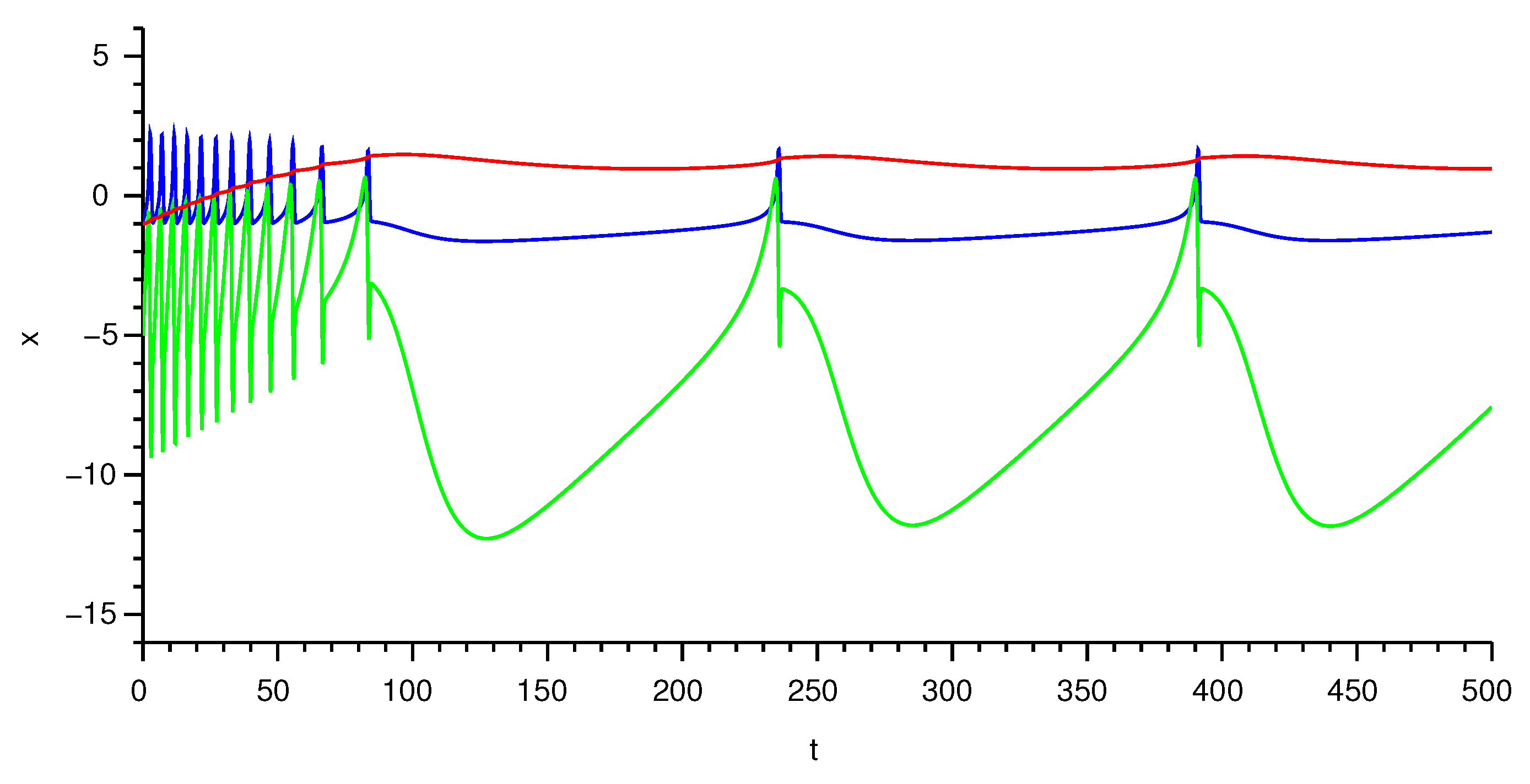
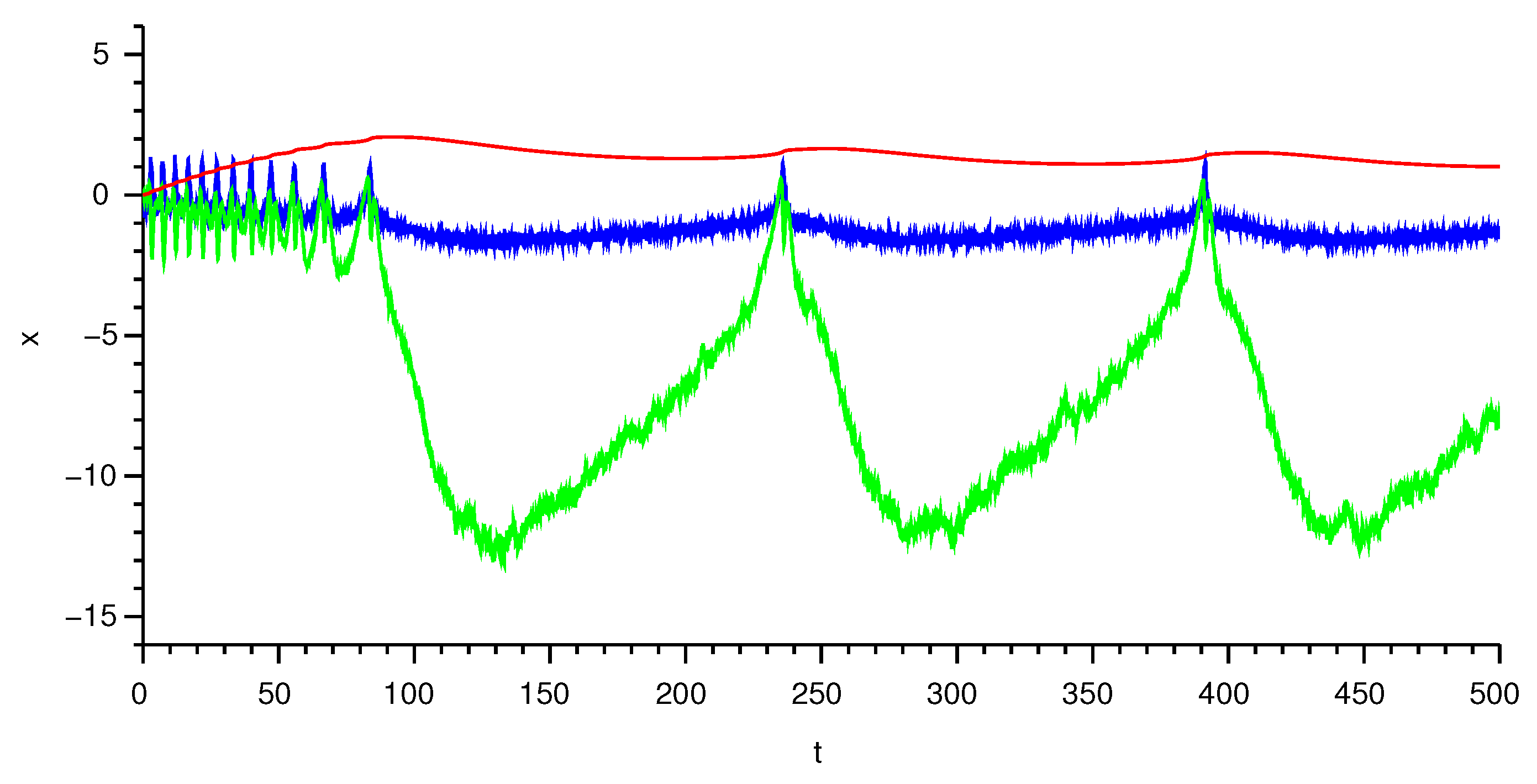
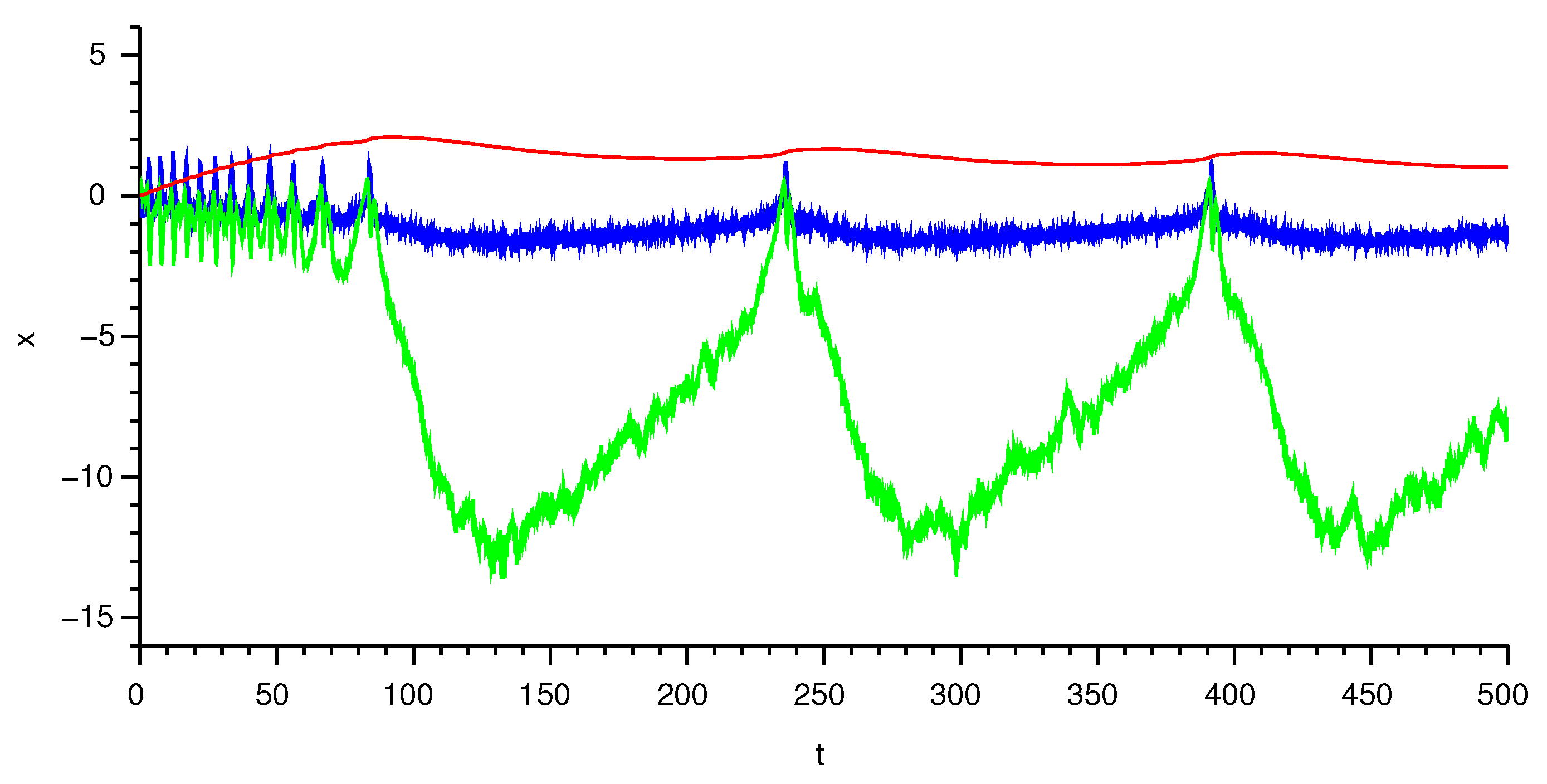
As can be seen from the equations describing the HR neuronal model, the non-observable part of the HR neuron is not controlled. However, Ref. [65] shows that these parts can be synchronized as well. It could be possible due to the fact that the HR neuron is a minimum-phase system. In the aforementioned paper, the proof of convergence of the non-observable parts for nonlinear zero dynamics is present. Its exponential stability is the only requirement. However, in the HR neuron, the zero dynamics is linear; hence, the result can be achieved in a simpler way and, moreover, it holds globally. The direct counterpart of Theorem 5.4 in [65] is

Theorem 3.

Suppose assumptions of Lemma 2 hold. Then, the non-observable part (13)–(15) is synchronized.

Proof. 

From (12), it follows that

$${\dot{\zeta }}_i-{\dot{\zeta }}_{i_0}=\left(\begin{array}{cc}-1& 0\\ 0& -0.006\end{array}\right)({\zeta }_i-{\zeta }_{i_0})+\left(\begin{array}{c}-({\eta }_i-{\eta }_{i_0})\\ c({\eta }_i-{\eta }_{i_0})\end{array}\right).$$

(51)

Theorem 2 implies that ${lim}_{t\to \infty }\mathbb{E}\left(\parallel {\eta }_i-{\eta }_{i_0}\parallel \right)=0$. This fact together with the exponential stability of the zero dynamics imply also

${lim}_{t\to \infty }\mathbb{E}\left(\parallel {\zeta }_i-{\zeta }_{i_0}\parallel \right)=0$. □

The main result can be formulated in the form of the following theorem.

Theorem 4.

Under assumptions of the Theorems 2 and 3, if the control input is defined by (16), then ${lim}_{t\to \infty }\mathbb{E}(\parallel x_i-x_{i_0}\parallel )=0$.

Proof. 

Theorem 3 implies that ${lim}_{t\to \infty }\mathbb{E}\left(\parallel {\zeta }_i-{\zeta }_{i_0}\parallel \right)=0$. The conclusion follows from the fact that the exact feedback linearization that converts the system (13)–(15) into (11) together with the control input transformation (10) is a diffeomorphism. □

Remark 5.

It is assumed that the transmission of information is subjected to time delay τ. Therefore, the delayed values $x_{1,j,\tau }$ are used to compute the control of the ith neuron. For the consistency, one has to use the value $x_{1,i,\tau }$ in the second term of (16) as well as the results of [26] to indicate that using $(x_{1,j,\tau }-x_{1,i})$ could lead to a synchronization error whose value would not be limited to zero. On the other hand, as it is assumed that $x_{1,i}$ is accessible to the ith agent, one can use this value in the term $F\left(x_i\right)$.

7. Example

Our theoretical results were used for a network consisting of six neurons with neuron 0 as a leader by the numerical simulations. All parameters are the same as in Section 4. The topology of the neuronal network is depicted in Figure 1.

From the topology of the network, with nodes being the neurons, it follows that one can take $D=\mathrm{diag}(0.2866,1.007,1.8044,2.435,2.689)$ which satisfies (1). Moreover, $\varkappa =0.5$, ${\varkappa }_1=7$, ${\varkappa }_2=33$. Furthermore, the parameter $\Sigma$ was chosen as $\Sigma =0.1$ and, finally, $r=200$. The maximal time delay was 0.1 s. After applying the LMI optimization procedure, one obtains $k=-6.94$.

The simulations were obtained using the Sundials-CVODE solver with backward differentiation. The Adams–Moulton with a variable step was used. Note that the variable step method, often causing problems in the case of numerical investigation of the chaotic systems, can be used here, as the neurons considered in this paper are not in the chaotic regime, due to the sufficiently low external current.

The following figures show the state of the neurons. Figure 2 shows the state of the leader neuron. In this case, there is no noise in order to show its “nominal” behavior. The meaning of the curves is as follows: the blue line represents the state of $x_1$, the green line stands for the variable $x_2$, and, finally, the red line illustrates the state of $x_3$. The same meaning has lines in Figure 3, which shows the state of neuron 1. Moreover, the state of the neuron 3 is depicted in Figure 4.

The difference $\sqrt{{\sum }_{i=1}^5{(x_{1,i}-x_{1,0})}^2}$ is depicted in Figure 5. Similarly, the difference $\sqrt{{\sum }_{i=1}^5(x_{2,i}-x_{2,0})}$ is shown in Figure 6 and $\sqrt{{\sum }_{i=1}^5(x_{3,i}-x_{3,0})}$ in Figure 7 (note the different time range in the latter figure). Since the synchronization is achieved only through the potential (state $x_1$), one can see that the synchronization is quite good in this state, up to the points where the rapid changes of the potential appear. The quality of the synchronization of this part is enhanced by exact matching of the nonlinearities expressed by the function F. Contrary to this, synchronization of the remaining two variables is achieved only through the stability of the zero dynamics of this part. This results in a slower synchronization and larger errors.

8. Conclusions

An algorithm for synchronization of a neuronal network composed of Hindmarsh–Rose neurons with noise was investigated. The synchronization of the observable part is achieved by solving a set of LMIs derived due to application of the Razumikhin theorem. The proof of synchronization of the non-observable part is based on the minimum-phase property of the Hindmarsh–Rose neurons. Viability of the algorithm is demonstrated by an example. In the future, synchronization of neuronal networks with different time delays will be investigated.

References

1. Erdös, P.; Rényi, A. On the evolution of random graphs. Publ. Math. Inst. Hung. Acad. Sci. 1960, 5, 17–61. [Google Scholar]
2. Boccaletti, S.; Pisarchik, A.; del Genio, C.; Amann, A. Synchronization: From Coupled Systems to Complex Networks; Cambridge University Press: Cambridge, UK, 2018. [Google Scholar]
3. Fujisaka, H.; Yamada, T. Stability Theory of Synchronized Motion in Coupled-Oscillator Systems. Prog. Theor. Phys. 1983, 69, 32–47. [Google Scholar] [CrossRef]
4. Pikovsky, A.S. On the interaction of strange attractors. Z. Phys. B Condens. Matter 1984, 55, 149–154. [Google Scholar] [CrossRef]
5. Pecora, L.M.; Carroll, T.L. Synchronization in chaotic systems. Phys. Rev. Lett. 1990, 64, 821–824. [Google Scholar] [CrossRef]
6. Rosenblum, M.G.; Pikovsky, A.S.; Kurths, J. Phase Synchronization of Chaotic Oscillators. Phys. Rev. Lett. 1996, 76, 1804–1807. [Google Scholar] [CrossRef] [PubMed]
7. Rulkov, N.F.; Sushchik, M.M.; Tsimring, L.S.; Abarbanel, H.D.I. Generalized synchronization of chaos in directionally coupled chaotic systems. Phys. Rev. E 1995, 51, 980–994. [Google Scholar] [CrossRef] [PubMed]
8. Kocarev, L.; Parlitz, U. Generalized Synchronization, Predictability, and Equivalence of Unidirectionally Coupled Dynamical Systems. Phys. Rev. Lett. 1996, 76, 1816–1819. [Google Scholar] [CrossRef] [PubMed] [Green Version]
9. Mainieri, R.; Rehacek, J. Projective Synchronization In Three-Dimensional Chaotic Systems. Phys. Rev. Lett. 1999, 82, 3042–3045. [Google Scholar] [CrossRef]
10. Rosenblum, M.G.; Pikovsky, A.S.; Kurths, J. From Phase to Lag Synchronization in Coupled Chaotic Oscillators. Phys. Rev. Lett. 1997, 78, 4193–4196. [Google Scholar] [CrossRef]
11. Plotnikov, S.A.; Fradkov, A.L. On synchronization in heterogeneous FitzHugh–Nagumo networks. Chaos Solitons Fractals 2019, 121, 85–91. [Google Scholar] [CrossRef]
12. Abarbanel, H.D.I.; Rulkov, N.F.; Sushchik, M.M. Generalized synchronization of chaos: The auxiliary system approach. Phys. Rev. E 1996, 53, 4528–4535. [Google Scholar] [CrossRef] [Green Version]
13. Lynnyk, V.; Rehák, B.; Čelikovský, S. On applicability of auxiliary system approach in complex network with ring topology. Cybern. Phys. 2019, 8, 143–152. [Google Scholar] [CrossRef] [Green Version]
14. Lynnyk, V.; Rehák, B.; Čelikovský, S. On detection of generalized synchronization in the complex network with ring topology via the duplicated systems approach. In Proceedings of the 8th International Conference on Systems and Control (ICSC), Marrakesh, Morocco, 23–25 October 2019. [Google Scholar]
15. Hramov, A.E.; Koronovskii, A.A.; Moskalenko, O.I. Generalized synchronization onset. Europhys. Lett. (EPL) 2005, 72, 901–907. [Google Scholar] [CrossRef] [Green Version]
16. Moskalenko, O.I.; Koronovskii, A.A.; Hramov, A.E. Generalized synchronization of chaos for secure communication: Remarkable stability to noise. Phys. Lett. A 2010, 374, 2925–2931. [Google Scholar] [CrossRef] [Green Version]
17. Zhou, J.; Chen, J.; Lu, J.; Lu, J. On Applicability of Auxiliary System Approach to Detect Generalized Synchronization in Complex Network. IEEE Trans. Autom. Control 2017, 62, 3468–3473. [Google Scholar] [CrossRef]
18. Karimov, A.; Tutueva, A.; Karimov, T.; Druzhina, O.; Butusov, D. Adaptive Generalized Synchronization between Circuit and Computer Implementations of the Rössler System. Appl. Sci. 2020, 11, 81. [Google Scholar] [CrossRef]
19. Koronovskii, A.A.; Moskalenko, O.I.; Pivovarov, A.A.; Khanadeev, V.A.; Hramov, A.E.; Pisarchik, A.N. Jump intermittency as a second type of transition to and from generalized synchronization. Phys. Rev. E 2020, 102, 012205. [Google Scholar] [CrossRef]
20. Lynnyk, V.; Čelikovský, S. Generalized synchronization of chaotic systems in a master–slave configuration. In Proceedings of the 2021 23rd International Conference on Process Control (PC), Strbske Pleso, Slovakia, 1–4 June 2021. [Google Scholar]
21. Lynnyk, V.; Čelikovský, S. Anti-synchronization chaos shift keying method based on generalized Lorenz system. Kybernetika 2010, 46, 1–18. [Google Scholar]
22. Čelikovský, S.; Lynnyk, V. Message Embedded Chaotic Masking Synchronization Scheme Based on the Generalized Lorenz System and Its Security Analysis. Int. J. Bifurc. Chaos 2016, 26, 1650140. [Google Scholar] [CrossRef]
23. Čelikovský, S.; Lynnyk, V. Lateral Dynamics of Walking-Like Mechanical Systems and Their Chaotic Behavior. Int. J. Bifurc. Chaos 2019, 29, 1930024. [Google Scholar] [CrossRef]
24. Karimov, T.; Butusov, D.; Andreev, V.; Karimov, A.; Tutueva, A. Accurate Synchronization of Digital and Analog Chaotic Systems by Parameters Re-Identification. Electronics 2018, 7, 123. [Google Scholar] [CrossRef] [Green Version]
25. Andrievsky, B. Numerical evaluation of controlled synchronization for chaotic Chua systems over the limited-band data erasure channel. Cybern. Phys. 2016, 5, 43–51. [Google Scholar]
26. Rehák, B.; Lynnyk, V. Synchronization of symmetric complex networks with heterogeneous time delays. In Proceedings of the 2019 22nd International Conference on Process Control (PC19), Strbske Pleso, Slovakia, 11–14 June 2019; pp. 68–73. [Google Scholar]
27. Rehák, B.; Lynnyk, V. Network-based control of nonlinear large-scale systems composed of identical subsystems. J. Frankl. Inst. 2019, 356, 1088–1112. [Google Scholar] [CrossRef]
28. Hramov, A.E.; Khramova, A.E.; Koronovskii, A.A.; Boccaletti, S. Synchronization in networks of slightly nonidentical elements. Int. J. Bifurc. Chaos 2008, 18, 845–850. [Google Scholar] [CrossRef] [Green Version]
29. Rehák, B.; Lynnyk, V. Decentralized networked stabilization of a nonlinear large system under quantization. In Proceedings of the 8th IFAC Workshop on Distributed Estimation and Control in Networked Systems (NecSys 2019), Chicago, IL, USA, 16–17 September 2019; pp. 1–6. [Google Scholar]
30. Boccaletti, S.; Kurths, J.; Osipov, G.; Valladares, D.; Zhou, C. The synchronization of chaotic systems. Phys. Rep. Rev. Sect. Phys. Lett. 2002, 366, 1–101. [Google Scholar] [CrossRef]
31. Chen, G.; Dong, X. From Chaos to Order; World Scientific: Singapore, 1998. [Google Scholar]
32. Rehák, B.; Lynnyk, V. Consensus of a multi-agent systems with heterogeneous delays. Kybernetika 2020, 56, 363–381. [Google Scholar] [CrossRef]
33. Rehák, B.; Lynnyk, V. Leader-following synchronization of a multi-agent system with heterogeneous delays. Front. Inf. Technol. Electron. Eng. 2021, 22, 97–106. [Google Scholar] [CrossRef]
34. Hu, M.; Guo, L.; Hu, A.; Yang, Y. Leader-following consensus of linear multi-agent systems with randomly occurring nonlinearities and uncertainties and stochastic disturbances. Neurocomputing 2015, 149, 884–890. [Google Scholar] [CrossRef]
35. Ren, H.; Deng, F.; Peng, Y.; Zhang, B.; Zhang, C. Exponential consensus of nonlinear stochastic multi-agent systems with ROUs and RONs via impulsive pinning control. IET Control Theory Appl. 2017, 11, 225–236. [Google Scholar] [CrossRef]
36. Ma, L.; Wang, Z.; Han, Q.L.; Liu, Y. Consensus control of stochastic multi-agent systems: A survey. Sci. China Inf. Sci. 2017, 60, 1869–1919. [Google Scholar] [CrossRef] [Green Version]
37. Čelikovský, S.; Lynnyk, V.; Chen, G. Robust synchronization of a class of chaotic networks. J. Frankl. Inst. 2013, 350, 2936–2948. [Google Scholar] [CrossRef]
38. Malik, S.; Mir, A. Synchronization of Hindmarsh Rose Neurons. Neural Netw. 2020, 123, 372–380. [Google Scholar]
39. Ngouonkadi, E.M.; Fotsin, H.; Fotso, P.L.; Tamba, V.K.; Cerdeira, H.A. Bifurcations and multistability in the extended Hindmarsh–Rose neuronal oscillator. Chaos Solitons Fractals 2016, 85, 151–163. [Google Scholar] [CrossRef] [Green Version]
40. Hodgkin, A.L.; Huxley, A. A quantitative description of membrane current and its application to conduction and excitation in nerve. J. Physiol. 1952, 117, 500–544. [Google Scholar] [CrossRef] [PubMed]
41. Ostrovskiy, V.; Butusov, D.; Karimov, A.; Andreev, V. Discretization effects during numerical investigation of Hodgkin-Huxley neuron model. Bull. Bryansk State Tech. Univ. 2019, 94–101. [Google Scholar] [CrossRef]
42. Andreev, V.; Ostrovskii, V.; Karimov, T.; Tutueva, A.; Doynikova, E.; Butusov, D. Synthesis and Analysis of the Fixed-Point Hodgkin-Huxley Neuron Model. Electronics 2020, 9, 434. [Google Scholar] [CrossRef] [Green Version]
43. FitzHugh, R. Impulses and Physiological States in Theoretical Models of Nerve Membrane. Biophys. J. 1961, 1, 445–466. [Google Scholar] [CrossRef] [Green Version]
44. Nagumo, J.; Arimoto, S.; Yoshizawa, S. An Active Pulse Transmission Line Simulating Nerve Axon. Proc. IRE 1962, 50, 2061–2070. [Google Scholar] [CrossRef]
45. Hindmarsh, J.; Rose, R. A model of neuronal bursting using three coupled first order differential equations. Proc. R. Soc. London Ser. B Contain. Pap. A Biol. Character. R. Soc. (Great Br.) 1984, 221, 87–102. [Google Scholar]
46. epek, M.; Fronczak, P. Spatial evolution of Hindmarsh–Rose neural network with time delays. Nonlinear Dyn. 2018, 92, 751–761. [Google Scholar]
47. Ding, K.; Han, Q.L. Master–slave synchronization criteria for chaotic Hindmarsh–Rose neurons using linear feedback control. Complexity 2016, 21, 319–327. [Google Scholar] [CrossRef]
48. Nguyen, L.H.; Hong, K.S. Adaptive synchronization of two coupled chaotic Hindmarsh–Rose neurons by controlling the membrane potential of a slave neuron. Appl. Math. Model. 2013, 37, 2460–2468. [Google Scholar] [CrossRef]
49. Ding, K.; Han, Q.L. Synchronization of two coupled Hindmarsh–Rose neurons. Kybernetika 2015, 51, 784–799. [Google Scholar] [CrossRef] [Green Version]
50. Hettiarachchi, I.T.; Lakshmanan, S.; Bhatti, A.; Lim, C.P.; Prakash, M.; Balasubramaniam, P.; Nahavandi, S. Chaotic synchronization of time-delay coupled Hindmarsh–Rose neurons via nonlinear control. Nonlinear Dyn. 2016, 86, 1249–1262. [Google Scholar] [CrossRef]
51. Equihua, G.G.V.; Ramirez, J.P. Synchronization of Hindmarsh–Rose neurons via Huygens-like coupling. IFAC-PapersOnLine 2018, 51, 186–191. [Google Scholar] [CrossRef]
52. Yu, H.; Peng, J. Chaotic synchronization and control in nonlinear-coupled Hindmarsh–Rose neural systems. Chaos Solitons Fractals 2006, 29, 342–348. [Google Scholar] [CrossRef]
53. Xu, Y.; Jia, Y.; Ma, J.; Alsaedi, A.; Ahmad, B. Synchronization between neurons coupled by memristor. Chaos Solitons Fractals 2017, 104, 435–442. [Google Scholar] [CrossRef]
54. Bandyopadhyay, A.; Kar, S. Impact of network structure on synchronization of Hindmarsh–Rose neurons coupled in structured network. Appl. Math. Comput. 2018, 333, 194–212. [Google Scholar] [CrossRef]
55. Ma, J.; Mi, L.; Zhou, P.; Xu, Y.; Hayat, T. Phase synchronization between two neurons induced by coupling of electromagnetic field. Appl. Math. Comput. 2017, 307, 321–328. [Google Scholar] [CrossRef]
56. Andreev, A.V.; Frolov, N.S.; Pisarchik, A.N.; Hramov, A.E. Chimera state in complex networks of bistable Hodgkin-Huxley neurons. Phys. Rev. E 2019, 100, 022224. [Google Scholar] [CrossRef]
57. Semenov, D.M.; Fradkov, A.L. Adaptive synchronization in the complex heterogeneous networks of Hindmarsh–Rose neurons. Chaos Solitons Fractals 2021, 150, 111170. [Google Scholar] [CrossRef]
58. Ma, Z.C.; Wu, J.; Sun, Y.Z. Adaptive finite-time generalized outer synchronization between two different dimensional chaotic systems with noise perturbation. Kybernetika 2017, 53, 838–852. [Google Scholar] [CrossRef] [Green Version]
59. Zhang, J.; Wang, C.; Wang, M.; Huang, S. Firing patterns transition induced by system size in coupled Hindmarsh–Rose neural system. Neurocomputing 2011, 74, 2961–2966. [Google Scholar] [CrossRef]
60. Plotnikov, S.A. Controlled synchronization in two FitzHugh-Nagumo systems with slowly-varying delays. Cybern. Phys. 2015, 4, 21–25. [Google Scholar]
61. Plotnikov, S.A.; Lehnert, J.; Fradkov, A.L.; Schöll, E. Adaptive Control of Synchronization in Delay-Coupled Heterogeneous Networks of FitzHugh–Nagumo Nodes. Int. J. Bifurc. Chaos 2016, 26, 1650058. [Google Scholar] [CrossRef] [Green Version]
62. Plotnikov, S.A.; Fradkov, A.L. Desynchronization control of FitzHugh-Nagumo networks with random topology. IFAC-PapersOnLine 2019, 52, 640–645. [Google Scholar] [CrossRef]
63. Djeundam, S.D.; Filatrella, G.; Yamapi, R. Desynchronization effects of a current-driven noisy Hindmarsh–Rose neural network. Chaos Solitons Fractals 2018, 115, 204–211. [Google Scholar] [CrossRef]
64. Rehák, B.; Lynnyk, V. Synchronization of nonlinear complex networks with input delays and minimum-phase zero dynamics. In Proceedings of the 2019 19th International Conference on Control, Automation and Systems (ICCAS), Jeju, Korea, 15–18 October 2019; pp. 759–764. [Google Scholar]
65. Rehák, B.; Lynnyk, V.; Čelikovský, S. Consensus of homogeneous nonlinear minimum-phase multi-agent systems. IFAC-PapersOnLine 2018, 51, 223–228. [Google Scholar] [CrossRef]
66. Rehák, B.; Lynnyk, V. Synchronization of a network composed of Hindmarsh-Rose neurons with stochastic disturbances. In Proceedings of the 6th IFAC Hybrid Conference on Analysis and Control of Chaotic Systems (Chaos 2021), Catania, Italy, 27–29 September 2021. [Google Scholar]
67. Ni, W.; Cheng, D. Leader-following consensus of multi-agent systems under fixed and switching topologies. Syst. Control Lett. 2010, 59, 209–217. [Google Scholar] [CrossRef]
68. Song, Q.; Liu, F.; Cao, J.; Yu, W. Pinning-Controllability Analysis of Complex Networks: An M-Matrix Approach. IEEE Trans. Circuits Syst. I Regul. Pap. 2012, 59, 2692–2701. [Google Scholar] [CrossRef]
69. Song, Q.; Liu, F.; Cao, J.; Yu, W. M-Matrix Strategies for Pinning-Controlled Leader-Following Consensus in Multiagent Systems With Nonlinear Dynamics. IEEE Trans. Cybern. 2013, 43, 1688–1697. [Google Scholar] [CrossRef] [PubMed]
70. Khalil, H. Nonlinear Systems; Prentice Hall: Upper Saddle River, NJ, USA, 2001. [Google Scholar]
71. Huang, L.; Deng, F. Razumikhin-type theorems on stability of stochastic retarded systems. Int. J. Syst. Sci. 2009, 40, 73–80. [Google Scholar] [CrossRef]
72. Zhou, B.; Luo, W. Improved Razumikhin and Krasovskii stability criteria for time-varying stochastic time-delay systems. Automatica 2018, 89, 382–391. [Google Scholar] [CrossRef] [Green Version]
73. Peng, C.; Tian, Y.C. Networked Hinf control of linear systems with state quantization. Inf. Sci. 2007, 177, 5763–5774. [Google Scholar] [CrossRef] [Green Version]
Figure 1. The topology of the network.
Mathematics 09 02625 g001
Figure 2. State of the leader neuron. Blue line: x 0 , 1 , green line: x 0 , 2 , red line: x 0 , 3 .
Mathematics 09 02625 g002
Figure 3. State of neuron 1. Blue line: x 1 , 1 , green line: x 1 , 2 , red line: x 1 , 3 .
Mathematics 09 02625 g003
Figure 4. State of neuron 3. Blue line: x 3 , 1 , green line: x 3 , 2 , red line: x 3 , 3 .
Mathematics 09 02625 g004
Figure 5. Norm of synchronization error in the membrane potential.
Mathematics 09 02625 g005
Figure 6. Norm of the synchronization error in the recovery variable.
Mathematics 09 02625 g006
Figure 7. Norm of the synchronization error in the adaptation variable.
Mathematics 09 02625 g007
Publisher’s Note: MDPI stays neutral with regard to jurisdictional claims in published maps and institutional affiliations.