
A Fast Fixed-Point Algorithm for Convex Minimization Problems and Its Application in Image Restoration Problems

Abstract
1. Introduction
- (i)
- is a lower semicontinuous function and proper convex from a Hilbert space H into ;
- (ii)
- is a convex differentiable function from H into with being ℓ-Lipschitz constant for some that is, for all
2. Preliminaries
3. Main Results
| Algorithm 1: (MSA): A modified S-algorithm. |
| Initial. Take arbitrarily and . Choose and . Step 1. Compute , and using: Then, update , and go to Step 1. |
- (i)
- ;
- (ii)
- ;
- (iii)
- .
| Algorithm 2: (FBMSA): A forward-backward modified S-algorithm. |
| Initial. Take arbitrarily and . Choose and Step 1. Compute and using: Then, update , and go to Step 1. |
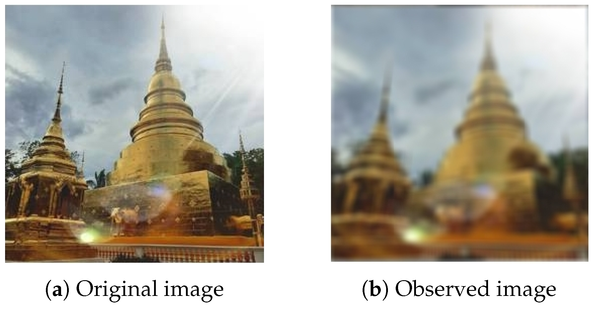
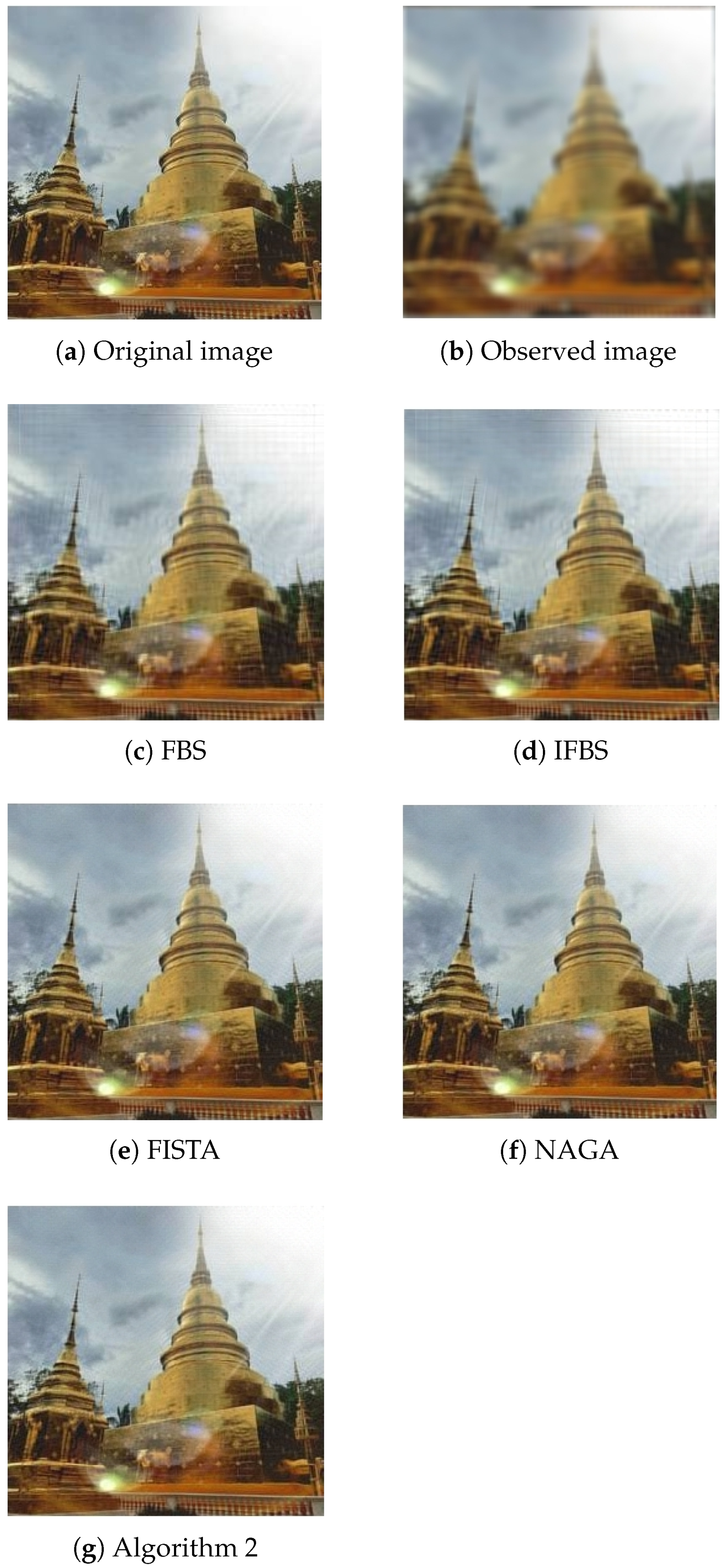
4. Applications
5. Conclusions
Author Contributions
Funding
Institutional Review Board Statement
Informed Consent Statement
Data Availability Statement
Acknowledgments
Conflicts of Interest
References
- Vogel, C.R. Computational Methods for Inverse Problems; SIAM: Philadelphia, PA, USA, 2002. [Google Scholar]
- Eld’en, L. Algorithms for the regularization of ill conditioned least squares problems. BIT Numer. Math. 1977, 17, 134–145. [Google Scholar] [CrossRef]
- Hansen, P.C.; Nagy, J.G.; O’Leary, D.P. Deblurring Images: Matrices, Spectra, and Filtering (Fundamentals of Algorithms 3) (Fundamentals of Algorithms); SIAM: Philadelphia, PA, USA, 2006. [Google Scholar]
- Tikhonov, A.N.; Arsenin, V.Y. Solutions of Ill-Posed Problems; VH Winston & Sons: Washington, DC, USA; John Wiley & Sons: New York, NY, USA, 1997. [Google Scholar]
- Tibshirain, R. Regression shrinkage abd selection via lasso. J. R. Stat. Soc. Ser. B (Method) 1996, 58, 267–288. [Google Scholar]
- Beck, A.; Teboulle, M. A fast iterative shrinkage-thresholding algorithm for linear inveerse problems. SIAMJ. Imaging Sci. 2009, 2, 183–202. [Google Scholar] [CrossRef]
- Bauschke, H.H.; Combettes, P.L. Convex Analysis and Monotone Operator Theory in Hilbert Spaces, 2nd ed.; Incorporated; Springr: New York, NY, USA, 2017. [Google Scholar]
- Parikh, N.; Boyd, S. Proximal Algorthims. Found. Trends R Optim. 2014, 1, 127–239. [Google Scholar] [CrossRef]
- Combettes, P.L. Quasi-Fejérian analysis of some optimization algorithms in Inherently Parallel Algorithms in Feasibility and Optimization and Their Applications. In Studies in Computational Mathematics; North-Holland: Amsterdam, The Netherlands, 2001; Volume 8, pp. 115–152. [Google Scholar]
- Combettes, P.L.; Pesquet, J.-C. Proximal splitting methods in signal processing. In Fixed-Point Algorithms for Inverse Problems. Science and Engineering; Springer Optimization and Its Applications: New York, NY, USA, 2011; Volume 49, pp. 185–212. [Google Scholar]
- Combettes, P.L.; Wajs, V.R. Signal recovery by proximal forward–backward splitting. Multiscale Model. Simul. 2005, 4, 1168–1200. [Google Scholar] [CrossRef]
- Lions, P.L.; Mercier, B. Splitting algorithms for the sum of two nonlinear operators. SIAM J. Numer. Anal. 1979, 16, 964–979. [Google Scholar] [CrossRef]
- Moreau, J.J. Proximité et dualité dans un espace hilbertien. Bull. Soc. Math. Fr. 1965, 93, 273–299. [Google Scholar] [CrossRef]
- Bussaban, L.; Suantai, S.; Kaewkhao, A. A parallel inertial S-iteration forward–backward algorithm for regression and classification problems. Carpathian J. Math. 2020, 36, 21–30. [Google Scholar] [CrossRef]
- Moudafi, A.; Oliny, M. Convergence of splitting inertial proximal method for monotone operators. J. Comput. Appl. Math. 2003, 155, 447–454. [Google Scholar] [CrossRef]
- Verma, M.; Shukla, K.K. A new accelerated proximal gradient technique for regularized multitask learning framework. Pattern Recogn. Lett. 2017, 95, 98–103. [Google Scholar] [CrossRef]
- Byrne, C. Iterative oblique projection onto convex subsets and the split feasibility problem. Inverse Probl. 2002, 18, 441–453. [Google Scholar] [CrossRef]
- Byrne, C. Aunified treatment of some iterative algorithms in signal processing and image reconstruction. Inverse Probl. 2004, 20, 103–120. [Google Scholar] [CrossRef]
- Cholamjiak, P.; Shehu, Y. Inertial forward–backward splitting method in Banach spaces with application to compressed sensing. Appl. Math. 2019, 64, 409–435. [Google Scholar] [CrossRef]
- Kunrada, K.; Pholasa, N.; Cholamjiak, P. On convergence and complexity of the modified forward–backward method involving new linesearches for convex minimization. Math. Meth. Appl. Sci. 2019, 42, 1352–1362. [Google Scholar]
- Suantai, S.; Eiamniran, N.; Pholasa, N.; Cholamjiak, P. Three-step projective methods for solving the split feasibility problems. Mathematics 2019, 7, 712. [Google Scholar] [CrossRef]
- Suantai, S.; Kesornprom, S.; Cholamjiak, P. Modified proximal algorithms for finding solutions of the split variational inclusions. Mathematics 2019, 7, 708. [Google Scholar] [CrossRef]
- Thong, D.V.; Cholamjiak, P. Strong convergence of a forward–backward splitting method with a new step size for solving monotone inclusions. Comput. Appl. Math. 2019, 38, 1–16. [Google Scholar] [CrossRef]
- Mann, W.R. Mean value methods in iteration. Proc. Am. Math. Soc. 1953, 4, 506–510. [Google Scholar] [CrossRef]
- Ishikawa, S. Fixed points by a new iteration method. Proc. Am. Math. Soc. 1974, 44, 147–150. [Google Scholar] [CrossRef]
- Phuengrattana, W.; Suantai, S. On the rate of convergence of Mann, Ishikawa, Noor and SP-iterations for continuousfunctions on an arbitrary interval. J. Comput. Appl. Math. 2011, 235, 3006–3014. [Google Scholar] [CrossRef]
- Hanjing, A.; Suthep, S. The split fixed-point problem for demicontractive mappings and applications. Fixed Point Theory 2020, 21, 507–524. [Google Scholar] [CrossRef]
- Wongyai, S.; Suantai, S. Convergence Theorem and Rate of Convergence of a New Iterative Method for Continuous Functions on Closed Interval. In Proceedings of the AMM and APAM Conference Proceedings, Bankok, Thailand, 23–25 May 2016; pp. 111–118. [Google Scholar]
- De la Sen, M.; Agarwal, R.P. Common fixed points and best proximity points of two cyclic self-mappings. Fixed Point Theory Appl. 2012, 2012, 1–17. [Google Scholar] [CrossRef][Green Version]
- Gdawiec, K.; Kotarski, W. Polynomiography for the polynomial infinity norm via Kalantari’s formula and nonstandard iterations. Appl. Math. Comput. 2017, 307, 17–30. [Google Scholar] [CrossRef]
- Shoaib, A. Common fixed point for generalized contraction in b-multiplicative metric spaces with applications. Bull. Math. Anal. Appl. 2020, 12, 46–59. [Google Scholar]
- Al-Mazrooei, A.E.; Lateef, D.; Ahmad, J. Common fixed point theorems for generalized contractions. J. Math. Anal. 2017, 8, 157–166. [Google Scholar]
- Kim, K.S. A Constructive scheme for a common coupled fixed-point problems in Hilbert space. Mathematics 2020, 8, 1717. [Google Scholar] [CrossRef]
- Polyak, B. Some methods of speeding up the convergence of iteration methods. USSR Comput. Math. Math. Phys. 1964, 4, 1–17. [Google Scholar] [CrossRef]
- Moudafi, A.; Al-Shemas, E. Simulataneous iterative methods for split equality problem. Trans. Math. Program. Appl. 2013, 1, 1–11. [Google Scholar]
- Nakajo, K.; Shimoji, K.; Takahashi, W. Strong convergence to common fixed points of families of nonexpansive mapping in Banach spaces. J. Nonlinear Convex Anal. 2007, 8, 11–34. [Google Scholar]
- Nakajo, K.; Shimoji, K.; Takahashi, W. On strong convergence by the hybrid method for families of mappings in Hilbert spaces. Nonlinear Anal. Theor. Methods Appl. 2009, 71, 112–119. [Google Scholar] [CrossRef]
- Takahashi, W. Introduction to Nonlinear and Convex Analysis; Yokohama Publishers: Yokohama, Japan, 2009. [Google Scholar]
- Takahashi, W. Nonlinear Functional Analysis; Yokohama Publishers: Yokohama, Japan, 2000. [Google Scholar]
- Tan, K.; Xu, H.K. Approximating fixed points of nonexpansive mappings by the ishikawa iteration process. J. Math. Anal. Appl. 1993, 178, 301–308. [Google Scholar] [CrossRef]
- Hanjing, A.; Suantai, S. A fast image restoration algorithm based on a fixed point and optimization method. Mathematics 2020, 8, 378. [Google Scholar] [CrossRef]
- Moreau, J.J. Fonctions convexes duales et points proximaux dans un espace hilbertien. C. R. Acad. Sci. Paris Sér. A Math. 1962, 255, 2897–2899. [Google Scholar]
- Thung, K.; Raveendran, P. A survey of image quality measures. In Proceedings of the International Conference for Technical Postgraduates (TECHPOS), Kuala Lumpur, Malaysia, 14–15 December 2009; pp. 1–4. [Google Scholar]


| Methods | Setting |
|---|---|
| Algorithm 2 | and |
| FISTA | where |
| NAGA | and where |
| IFBS | and |
| FBS |
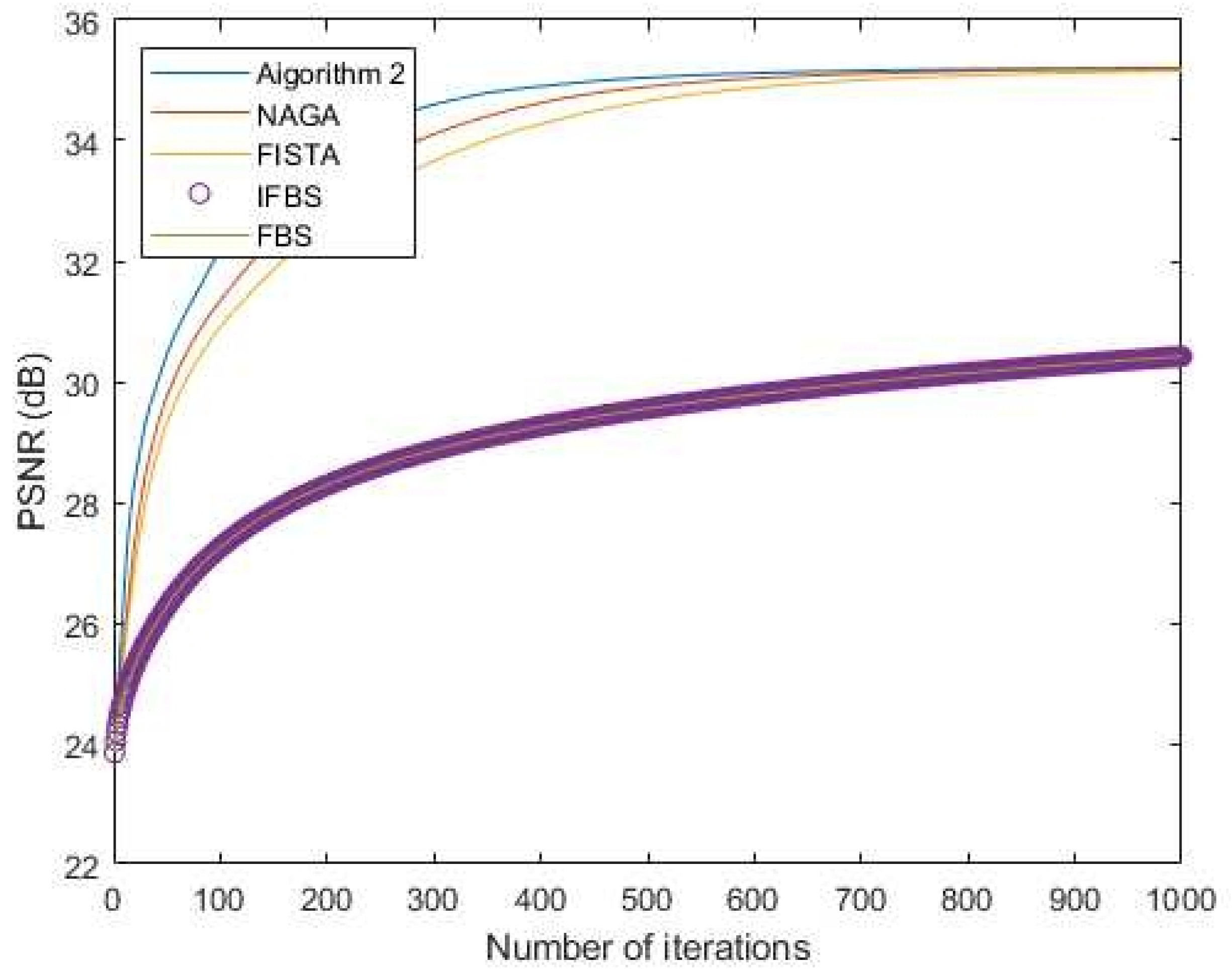
| Iteration No. | Peak Signal-to-Noise Ratio (PSNR) | ||||
|---|---|---|---|---|---|
| Algorithm 2 | NAGA | FISTA | IFBS | FBS | |
| 200 | 33.8764 | 33.1457 | 32.6173 | 28.2840 | 28.2840 |
| 300 | 34.5951 | 34.1018 | 33.6556 | 28.8650 | 28.8650 |
| 400 | 34.8902 | 34.6174 | 34.2689 | 29.2593 | 29.2593 |
| 500 | 35.0391 | 34.8766 | 34.6409 | 29.5532 | 29.5532 |
| 1000 | 35.2068 | 35.1961 | 35.1562 | 30.4187 | 30.4186 |
Publisher’s Note: MDPI stays neutral with regard to jurisdictional claims in published maps and institutional affiliations. |
© 2021 by the authors. Licensee MDPI, Basel, Switzerland. This article is an open access article distributed under the terms and conditions of the Creative Commons Attribution (CC BY) license (https://creativecommons.org/licenses/by/4.0/).
Share and Cite
Thongpaen, P.; Wattanataweekul, R. A Fast Fixed-Point Algorithm for Convex Minimization Problems and Its Application in Image Restoration Problems. Mathematics 2021, 9, 2619. https://doi.org/10.3390/math9202619
Thongpaen P, Wattanataweekul R. A Fast Fixed-Point Algorithm for Convex Minimization Problems and Its Application in Image Restoration Problems. Mathematics. 2021; 9(20):2619. https://doi.org/10.3390/math9202619
Chicago/Turabian StyleThongpaen, Panadda, and Rattanakorn Wattanataweekul. 2021. "A Fast Fixed-Point Algorithm for Convex Minimization Problems and Its Application in Image Restoration Problems" Mathematics 9, no. 20: 2619. https://doi.org/10.3390/math9202619
APA StyleThongpaen, P., & Wattanataweekul, R. (2021). A Fast Fixed-Point Algorithm for Convex Minimization Problems and Its Application in Image Restoration Problems. Mathematics, 9(20), 2619. https://doi.org/10.3390/math9202619