Marginalized Two-Part Joint Modeling of Longitudinal Semi-Continuous Responses and Survival Data: With Application to Medical Costs

Abstract

Non-negative continuous outcomes with a substantial number of zero values and incomplete longitudinal follow-up are quite common in medical costs data. It is thus critical to incorporate the potential dependence of survival status and longitudinal medical costs in joint modeling, where censorship is death-related. Despite the wide use of conventional two-part joint models (CTJMs) to capture zero-inflation, they are limited to conditional interpretations of the regression coefficients in the model’s continuous part. In this paper, we propose a marginalized two-part joint model (MTJM) to jointly analyze semi-continuous longitudinal costs data and survival data. We compare it to the conventional two-part joint model (CTJM) for handling marginal inferences about covariate effects on average costs. We conducted a series of simulation studies to evaluate the superior performance of the proposed MTJM over the CTJM. To illustrate the applicability of the MTJM, we applied the model to a set of real electronic health record (EHR) data recently collected in Iran. We found that the MTJM yielded a smaller standard error, root-mean-square error of estimates, and AIC value, with unbiased parameter estimates. With this MTJM, we identified a significant positive correlation between costs and survival, which was consistent with the simulation results.

1. Introduction

In many medical studies, the measurement of the primary outcome may be via a semi-continuous random variable that combines a continuous distribution with point masses at one or more locations [1]. A particular type of semi-continuous outcome is characterized by a point mass at zero and positive values that usually follow a skewed distribution [2]. Examples include alcohol use, driving-simulator-based research, annual medical costs, etc. [3,4,5]. For instance, in medical-insurance-based economic applications, medical costs typically include a large number of zero values representing a population of “non-users” who do not benefit from the medical care system in a given time interval, and a continuous distribution representing the cost levels of those who do receive care [6,7].

Two-part models are often used to analyze such semi-continuous data. These models consist of two separate model parts, with part I to model the zero values and part II to model the continuous values. In fact, some researchers have shown an increased interest in analyzing the semi-continuous outcomes by modeling the discrete zero component separately from the nonzero continuous component [4]. More recently, accommodating longitudinal data has necessitated the extension of these two-part models, with researchers jointly modeling these two outcomes for valid and efficient inference. It has been suggested that ignoring the potential dependency between the components can lead to biased results [2,5,8].

Although still extensively used, the conventional two-part models (CTMs) for capturing zero-inflation are limited to conditional interpretations of the regression coefficients in the model’s continuous part. Expressly, they exclude zero values from the second component, and they only provide inferences on the subpopulation of those with positive outcomes. When doing so, a generalization of the results for the effects of covariates that are included in the continuous part of model is only applicable to “users” (e.g., those positive values). Marginal inferences on the populations of health care users and non-users cannot be easily obtained using the conventional two-part model [7]. Moreover, in longitudinal studies, the population of health care users is not fixed over time, whereas the inferences from conventional two-part models are made based on a fixed population [9].

To enhance such marginal inferences, marginalized two-part (MTP) models are preferable for longitudinal semi-continuous data [7]; they yield more interpretable estimates when the primary focus is to estimate covariate effects on the average costs across the entire population of both users and non-users. These models retain many of the most significant features of conventional two-part models, such as capturing zero-inflation and skewness. Still, they allow investigators to examine covariate effects on the overall mean—one of the primary targets in many applications [7,9]. Numerous studies have attempted to explain the importance of using marginalized two-part models to accurately model semi-continuous data from complex surveys [4,10,11]. Thus far, this method has not been applied to joint models of longitudinal and survival data, which is the aim of this paper.

Moreover, in health economics studies, patients are monitored longitudinally, and their medical costs are gathered until death or incomplete follow-up occurs. Particularly, this terminal event changes the repeated measures process afterward [12]. For example, death precludes further accumulation of medical costs—therefore, the repeated measures of medical costs (e.g., monthly medical costs) are zero after death [13]. In such cases, the repeated measures and time-to-event outcomes are not independent. Ignoring this possible correlation can result in biased parameter estimates and inefficient statistical inference [13,14]. In a variety of public health applications, the joint modeling of these two processes is a useful tool for considering the possible correlation between the longitudinal and survival outcomes [15,16].

Added to this correlation, as mentioned previously, the distribution of medical costs data is generally right-skewed, and includes a substantial number of zero values. An appropriate model, therefore, must take all of these aspects into consideration [17]. Liu et al., and Xu et al., proposed two-part joint models of these semi-continuous data. However, they used a CTP model for the longitudinal part, so they did not obtain the marginal inference for the continuous part of the models for the longitudinal part [13,14]. However, there have been no studies that join MTP and survival models. In this paper, we propose a new extension of a marginalized two-part model for a joint analysis of longitudinal and survival data that accounts for the semi-continuous nature of longitudinal medical costs data. This new method readily allows investigators to obtain marginal inferences for the entire population of heath care users and non-users. Considering that there is no closed form of the likelihood function, we use approximate maximum likelihood estimation with the Gaussian–Hermite quadrature method to make statistical inferences based on the new model. The analysis of medical costs data lies at the core of our motivation for attempting to conduct this study. Since these data are often highly skewed to the right, with a large proportion of patients having zero costs, together with censoring due to lack of follow-up or death, the distributional features of such medical costs data make modeling challenging from a methodological standpoint.

The remainder of this paper is arranged as follows: Section 2 briefly reviews the conventional two-part model for the joint analysis of longitudinal semi-continuous data and survival data, along with the new marginalized two-part joint model. A series of simulation studies is presented in Section 3 to investigate the performance of the proposed marginalized two-part joint model (MTJM). In addition, Section 3 presents an application of this new MTJM to electronic health record (EHR) data in Iran. Finally, Discussions are provided in Section 4 and conclusions in Section 5.

2. Materials and Methods

In this section, we describe the methods in detail.

2.1. Conventional Two-Part Model for Joint Analysis of Longitudinal Semi-Continuous Data and Survival Data

Suppose that the monthly medical costs for the $j$-th observation of subject $i$ ($i=1, 2, \dots , n)$ at time $t_{ij}$ ($j=1, 2, \dots , n_i)$ are denoted by $Y_{ij}$ (i.e., semi-continuous repeated measures), where $n$ is the total number of subjects, and $n_i$ is the number of measurements for the $i$-th subject. For each subject, consider a random censoring time $C_i$ and a random terminal event (death) time $D_i$ such that the repeated measures process is terminated at ${\tau }_i=min\left(C_i, D_i\right)$. Additionally, let ${\Delta }_i=I(D_i<C_i)$ denote an indicator variable, and assume that the deaths and censoring times are both continuous and independent. Moreover, let $x_{ij}$ denote the vector of covariates corresponding to the repeated measure for subject $i$ at time $j$, and $z_{it}$ the vector of covariates corresponding to the terminal event for subject i. Let ${\lambda }_i\left(t\right)$ denote the hazard for the terminal event.

To specify the semi-continuous nature of $Y_{ij}$, consider two groups of subjects, with group 1 for those with zero costs, and group 2 for those with positive costs. The probability that a subject belongs to group 2, and the parameters associated with the level of costs to some explanatory variables during repeated measurements, can be considered as common random variables, denoted by $a_i$, to capture the variability of subject effects. Since there might be subject effects with regard to hazard rates, we consider common random variables, denoted by $b_i$, to capture the correlations between hazard rates and costs.

With these notations, the conventional two-part joint model (CTJM) proposed by Liu et al. [14] can be defined as:

$${\eta }_{ij}^C=\mathrm{logit}\left({\pi }_{ij}\right)=x_{ij}^{\prime }{\mathbf{\alpha }}^{\mathit{C}}+a_i^C$$

(1)

$${\mu }_{ij}=E\left(\log \left( Y_{ij}|Y_{ij}>0, x_{ij},a_i^C,b_i^C\right)\right)=x_{ij}^{\prime }{\mathbf{\beta }}^{\mathit{C}}+{\delta }_1^C{a}_i^C+b_i^C$$

(2)

$${\lambda }_i^C\left(t\right)={\lambda }_0\left(t\right)\exp \left(z_{it}^{\prime }{\mathbf{\gamma }}^{\mathit{C}}+{\delta }_2^C{a}_i^C+{\delta }_3^C{b}_i^C\right)$$

(3)

where ${\pi }_{ij}=P(Y_{ij}>0|x_{ij},a_i^C, t_{ij}<D_i)$ is the probability that subject $i$ has positive costs at time $t_{ij}$, given all associated covariates, and ${\mu }_{ij}$ is the logarithm of the costs for subject $i$. Moreover, consider ${\lambda }_0\left(t\right)$ as the baseline hazard function for the terminal event. In addition, ${\mathbf{\alpha }}^{\mathit{C}}$, ${\mathbf{\beta }}^{\mathit{C}}$, ${\mathbf{\gamma }}^{\mathit{C}}$, ${\delta }_1^C$, ${\delta }_2^C$, and ${\delta }_3^C$ are unknown parameters. The subject-specific random effects $c_i^C=\left(a_i^C, b_i^C\right)~N\left(\mathbf{0}, \left[\begin{array}{cc}{\sigma }_a^2& {\sigma }_{ab}\\ {\sigma }_{ab}& {\sigma }_b^2\end{array}\right]\right)$ correlate the odds of having positive costs, the level of positive costs, and the survival. As discussed in Liu et al. [14], more complicated random effects—such as a random slope—can be easily incorporated into these equations if necessary. In Equations (1) and (2), ${\eta }_{ij}^C$ and ${\mu }_{ij}$ can be considered only when a patient is still alive. Naturally, the monthly medical costs after death are zero. In a recent study, Rustand et al. [1] further developed this CTJM to analyze longitudinal semi-continuous biomarkers and terminal events from metastatic colorectal cancer data.

2.2. Marginalized Two-Part Joint Model for Longitudinal Semi-Continuous Data and Survival Data

Extending the conventional two-part joint model (CTJM) proposed by Liu et al. [14] and Rustand et al. [1], which has been widely used to jointly model semi-continuous data and survival outcomes, we propose a more flexible marginalized two-part joint model (MTJM) by using marginalized two-part (MTP) models instead of conventional two-part (CTP) models for the longitudinal part. This newly proposed MTJM is also an extension of the work of Smith et al. [9], where they considered only the marginalized two-part model for longitudinal medical costs data, without considering the survival data (i.e., without joint modeling).

2.2.1. Marginalized Two-Part Model for Longitudinal Semi-Continuous Data

The general form of the probability density functions (PDFs) for the CTP model [9] is given by:

$$g_{CTP}\left(y_{ij}\right)=\{\begin{array}{ll}1-{\pi }_{ij}, \hfill & if y_{ij}=0\hfill \\ {\pi }_{ij}f\left(y_{ij};x_{ij}^{\prime }{\mathbf{\beta }}^{\mathit{C}}\right),\hfill & if y_{ij}>0\hfill \end{array}$$

(4)

where the probability of observing a non-zero cost—i.e., ${\pi }_{ij}$—can be modeled using a logit link:

$${\eta }_{ij}^C=\mathrm{logit}\left({\pi }_{ij}\right)=x_{ij}^{\prime }{\mathbf{\alpha }}^{\mathit{C}}+a_i^C$$

and the location parameter ${\mu }_{ij}$ from the positive values can be modeled in the second part of the CTP model assuming a log link:

$${\mu }_{ij}=E\left(\log \left(Y_{ij}|Y_{ij}>0, x_{ij}, a_i^C,b_i^C\right)\right)=x_{ij}^{\prime }{\mathbf{\beta }}^{\mathit{C}}+{\delta }_1^C{a}_i^C+b_i^C.$$

Under this parameterization, ${\mathbf{\beta }}^{\mathit{C}}$ lacks a meaningful interpretation in many conditions. Often, greater interest lies in estimating the effects of covariates on the marginal mean of $y_{ij}$ on the original scale for the overall population of users and non-users. For example, investigators are interested in examining the association between treatment and average costs among health care users and non-users. The conventional two-part model poses challenges to the estimation of this effect [7,9,18,19]. Therefore, a flexible two-part model remains necessary to accommodate dependence between components, while providing an interpretable parameterization of the marginal mean in longitudinal studies.

Smith et al. [9] proposed a novel marginalized two-part (MTP) longitudinal model in order to alleviate the limitations posed by the CTP model, directly parameterizing the effect of covariates on the marginal mean of $Y_{ij}$.

The MTP model has the same two-part structure as the conventional model, but rather than parameterizing the model in terms of ${\mu }_{ij}$—the log-scale location parameter of the conditionally positive values—the model is parameterized in terms of ${\nu }_{ij}=E\left(Y_{ij}\right)$—the overall mean from the combined population of users and non-users. Therefore, for the MTP model, the general form of the PDF [9] can be written as:

$$g_{MTP}\left(y_{ij}\right)=\{\begin{array}{ll}1-{\pi }_{ij}, \hfill & if y_{ij}=0\hfill \\ {\pi }_{ij}f\left(y_{ij};x_{ij}^{\prime }{\mathbf{\beta }}^{\mathit{M}}\right),\hfill & if y_{ij}>0\hfill \end{array}$$

The MTP model specifies the linear predictors:

$${\eta }_{ij}^M=\mathrm{logit}\left({\pi }_{ij}\right)=x_{ij}^{\prime }{\mathbf{\alpha }}^{\mathit{M}}+a_i^M$$

$$E\left(Y_{ij}|x_{ij}, a_i^M,b_i^M\right)=\exp \left(x_{ij}^{\prime }{\mathbf{\beta }}^{\mathit{M}}+{\delta }_1^M{a}_i^M+b_i^M\right)={\nu }_{ij}.$$

Under this parameterization, ${\mathbf{\beta }}^{\mathit{M}}$ is estimated for the entire population, while ${\mathbf{\beta }}^{\mathit{C}}$ is conditional on $Y_{ij}>0$.

2.2.2. Parameter Estimation of the Marginalized Two-Part Joint Model (MTJM)

We extend the previously proposed model to accommodate longitudinal semi-continuous and survival responses. We specify the general form of the marginalized two-part joint model based on CTJM, as before:

$${\eta }_{ij}^M=\mathrm{logit}\left({\pi }_{ij}\right)=x_{ij}^{\prime }{\mathbf{\alpha }}^{\mathit{M}}+a_i^M,$$

(5)

$${\nu }_{ij}=E\left(Y_{ij}|x_{ij}, a_i^M,b_i^M\right)=\exp \left(x_{ij}^{\prime }{\mathbf{\beta }}^{\mathit{M}}+{\delta }_1^M{a}_i^M+b_i^M\right),$$

(6)

$${\lambda }_i^M\left(t\right)={\lambda }_0\left(t\right)\exp \left\{z_{it}^{\prime }{\mathbf{\gamma }}^{\mathit{M}}+{\delta }_2^M{a}_i^M+{\delta }_3^M{b}_i^M\right\}.$$

(7)

The common random variables, denoted by $a_i^M$ and $b_i^M$, capture the variability of subject effects and the correlations between hazard rates and costs, respectively. It is important to note that, with the MTJP model, the parameter ${\mathbf{\beta }}^{\mathit{M}}$ in Equation (6) is interpreted differently from the parameter ${\mathbf{\beta }}^{\mathit{C}}$ in the CTJP model. In the CTJP model, the parameter ${\mathbf{\beta }}^{\mathit{C}}$ in Equation (2) is conditional on $Y_{ij}>0$, which means that the parameter ${\mathbf{\beta }}^{\mathit{C}}$ considers the effect of covariates for the subpopulation with positive costs. However, in the MTJP model, the parameter ${\mathbf{\beta }}^{\mathit{M}}$ in Equation (6) is estimated for the whole population with positive costs in the CTJP model, as well as the subpopulation with zero costs that is not included in the CTJP model. Using the MTP model as parameterized, ${\mathbf{\beta }}^{\mathit{M}}$ in Equation (6) is estimated for the entire population, while ${\mathbf{\beta }}^{\mathit{C}}$ in Equation (2) is conditional on $Y_{ij}>0$. Using log-normal distribution for $f(.)$ in Equation (4), the overall marginal mean ${\nu }_{ij}$ can be defined as:

$${\nu }_{ij}=E\left(Y_{ij}|x_{ij}, a_i^M,b_i^M\right)={\pi }_{ij}\exp \left({\mu }_{ij}+{\sigma }^2/2\right),$$

so

$$\begin{gathered} {\mu }_{ij}=E\left(\log (Y_{ij}|Y_{ij}>0, x_{ij}, a_i^C,b_i^C)\right)=\ln \left({\nu }_{ij}\right)-\ln \left({\pi }_{ij}\right)-{\sigma }^2/2 \\ =x_{ij}^{\prime }{\mathbf{\beta }}^{\mathit{M}}+{\delta }_1^M{a}_i^M+b_i^M-\ln \left({\pi }_{ij}\right)-{\sigma }^2/2. \end{gathered}$$

where $\sigma$ is the shape parameter in log-normal distribution. With the model formulation in MTJM, the likelihood for the $i$th subject is:

$$L_i\left(\mathbf{\omega }\right)={{\displaystyle \int }}^{}{{\displaystyle \int }}^{}\exp \left(l_i^A\right)\exp \left(l_i^B\right)\exp \left(l_i^C\right)p\left(c_i^M\right)d{c}_i^M,$$

where $\mathbf{\omega }$ is the vector of parameters including ${\mathbf{\alpha }}^{\mathit{M}}$, ${\mathbf{\beta }}^{\mathit{M}}$, ${\mathbf{\gamma }}^{\mathit{M}}$, ${\delta }_1^M$, ${\delta }_2^M$, and ${\delta }_3^M$, and $p\left(c_i^M\right)$ is the density function for $c_i^M=\left(a_i^M,b_i^M\right)~N\left(\mathbf{0},\left[\begin{array}{cc}{\sigma }_a^2& {\sigma }_{ab}\\ {\sigma }_{ba}& {\sigma }_b^2\end{array}\right]\right)$. The first part of the integral results from the odds of having positive costs, and constitutes part I of the two-part model:

$$l_i^A={\displaystyle \sum }_{j=1}^{n_i}\left[I_{ij}\log {\pi }_{ij}+\left(1-I_{ij}\right)\log \left(1-{\pi }_{ij}\right)\right]={\displaystyle \sum }_{j=1}^{n_i}\left[I_{ij}{\eta }_{ij}^M+\log \left(1-{\pi }_{ij}\right)\right],$$

where $I_{ij}$ is 1 if $Y_{ij}>0$, and 0 otherwise.

The amount of positive medical costs per month constitutes the second part:

$$l_i^B={\displaystyle \sum }_{j=1}^{n_i}{I}_{ij}\left\{-\ln y_{ij}-\frac{1}{2}\ln 2\pi +\ln \left(\sigma \right)-\frac{1}{2{\sigma }^2}{\left(\ln y_{ij}-{\mu }_{ij}\right)}^2\right\},$$

and the likelihood of death is:

$$l_i^C={\Delta }_i\left(\log f_i\left(t\right)\right)+\left(1-{\Delta }_i\right)\log \left(s_i\left(t\right)\right),$$

where

$$s_i\left(t\right)=\exp \left(-{\lambda }_i^M\left(t\right)\times t\right),$$

$$f_i\left(t\right)={\lambda }_i^M\left(t\right)\exp \left(-{\lambda }_i^M\left(t\right)\times t\right),$$

$${\lambda }_i^M\left(t\right)={\lambda }_0\left(t\right)\exp \left\{z_{it}^{\prime }{\mathbf{\gamma }}^{\mathit{M}}+{\delta }_2^M{a}_i^M+{\delta }_3^M{b}_i^M\right\}.$$

There is no analytical solution to obtain parameter estimates. Therefore, we adopt an adaptive Gaussian quadrature technique that can be implemented conveniently using the SAS procedure NLMIXED (SAS Program in Appendix A and Appendix B). In many real-life applications, nonlinear models are required that allow the investigators to specify parameters to the model individually and nonlinearly. For example, in some repeated measurements, it is of interest to fit a model that simultaneously accounts for the overall nonlinear mean structure as well as the variability between and within subjects. In this situation, nonlinear mixed-effects models can be useful, and the fitting of nonlinear mixed-effects models using the SAS procedure “PROC NLMIXED” can be the first choice. PROC NLMIXED fits nonlinear mixed-effects models by numerically maximizing an approximation to the marginal likelihood—that is, the likelihood integrated over the random effects [20,21].

3. Results

This section is divided into simulation study and real data study.

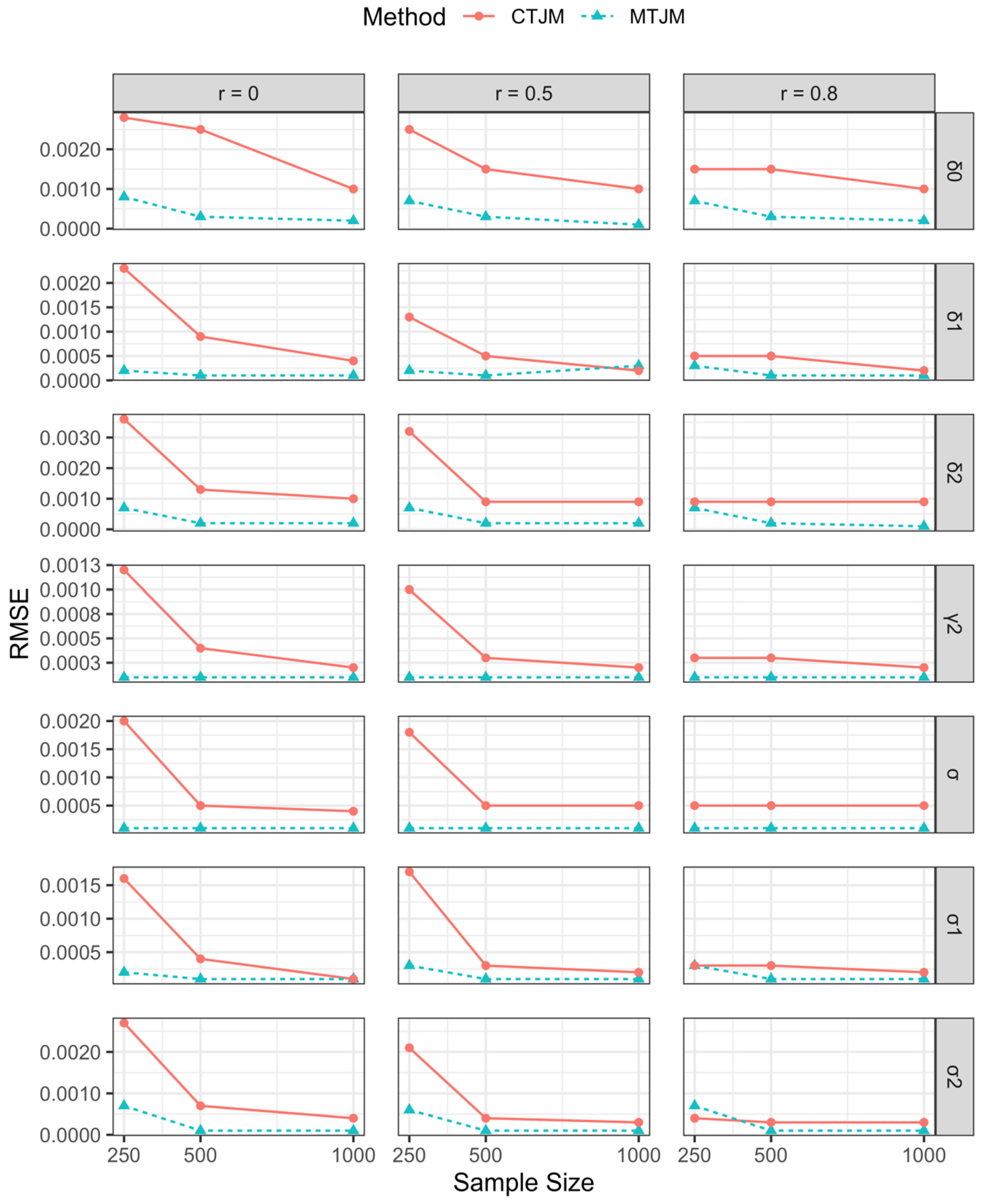
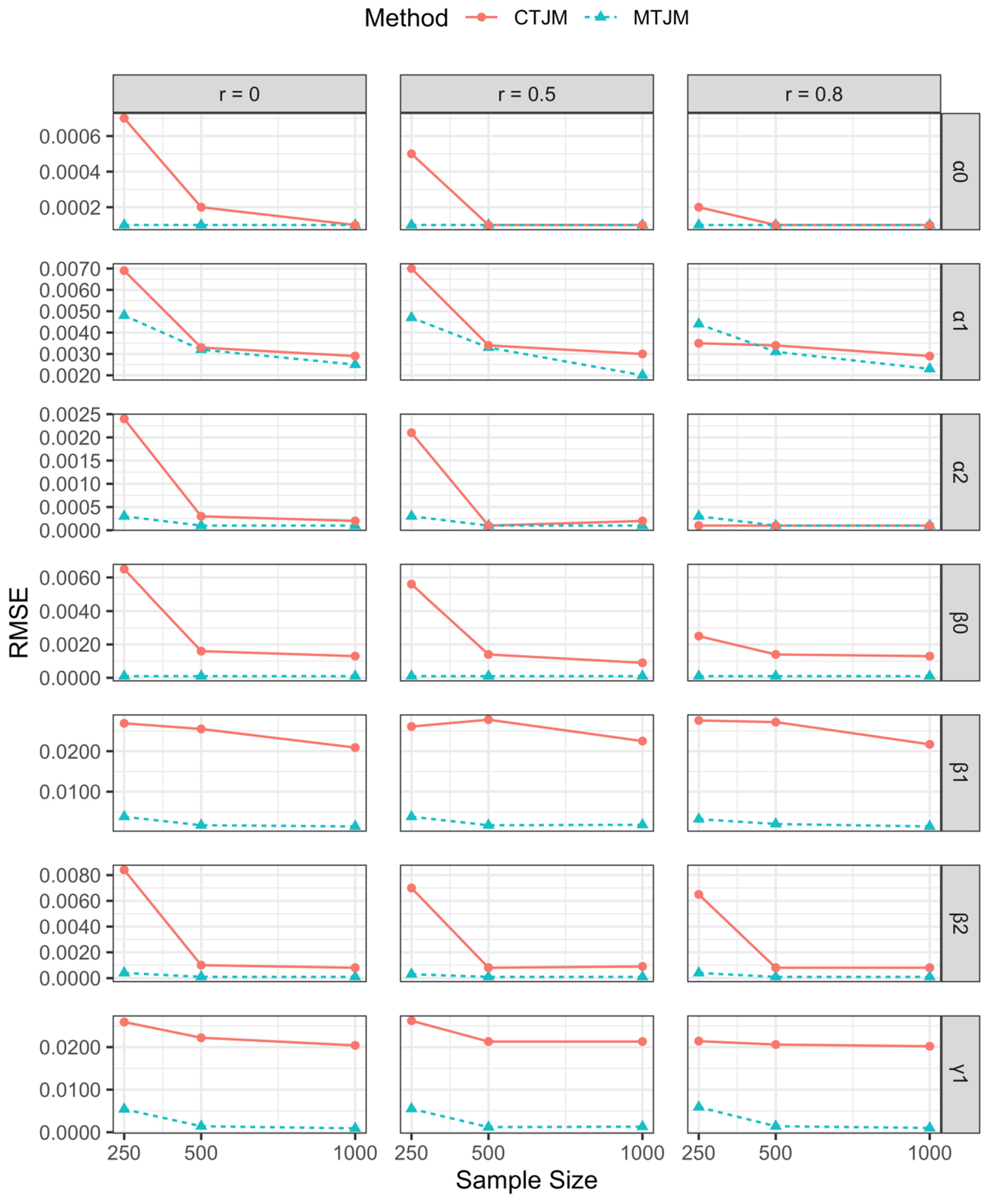
3.1. Simulation Study

In order to validate the proposed MTJM model, a simulation study was designed for the proposed estimation procedure performance to be examined. Repeated measures (such as monthly medical costs) are assumed for subject $i=1,\dots , n$ at the integer “time” (the month, for example), $j=0, \dots , n_i$ with the baseline of month 0. Data are simulated using the following model:

$${\eta }_{ij}^M=\mathrm{logit}\left({\pi }_{ij}\right)={\alpha }_0^M+x_{1ij}{\alpha }_1^M+x_{2ij}{\alpha }_2^M+a_i^M$$

$${\nu }_{ij}=\exp \left({\beta }_0^M+x_{1ij}{\beta }_1^M+x_{2ij}{\beta }_2^M+{\delta }_1{a}_i^M+b_i^M-\log \left({\pi }_{ij}\right)-{\sigma }^2/2\right)$$

$${\lambda }_i^M\left(t\right)=\exp \left\{z_{1it}{\gamma }_1^M+z_{2it}{\gamma }_2^M+{\delta }_2^M{a}_i^M+{\delta }_3^M{b}_i^M\right\}.$$

The first time-variant covariate $x_{1ij}=z_{1it}$ is simulated from the Bernoulli (p = 0.5) distribution, and the second time-variant covariate $x_{2ij}=z_{2it}$ is simulated from a standard normal distribution. The fixed-effects coefficients are set to ${\mathbf{\alpha }}^{\mathit{M}\mathbf{\prime }}=\left(14.4,-0.3, 1.6\right)$ and ${\mathbf{\beta }}^{\mathit{M}\mathbf{\prime }}=\left(5, 0.05, 1.1\right)$. These values, and the coding of the covariates, are obtained from the literature [7]. Additionally, in order to compare the performance between the MTJM and CTJM, we used simulation codes from previous works [13,14] for the CTJM. We take USD 1 as the monthly medical cost’s unit. We assume that the positive costs follow a log-normal distribution with ${\sigma }^2=4$. The hazard rate of subject i at time t follows an exponential distribution $E\left({\lambda }_i\left(t\right)\right)$. The parameter $\mathbf{\gamma }$ is a vector of coefficient of covariates, and it is assumed to be ${\mathbf{\gamma }}^{\mathit{M}\mathbf{\prime }}=\left(0.1,-1\right)$.

The independent censoring occurs from time 1 to time 4, with censoring probabilities of 2% (at time 1), 3% (at time 2), 15% (at time 3), and 80% (at time 4). The follow-up of repeated measures is not available after either death or independent censoring. The times of censoring are set independently to the exponential distribution E(1).

Independent random intercepts $a_i$ and $b_i$ are considered in the model. We assume that the random effects jointly follow a bivariate normal distribution with mean 0 and variance–covariance matrix $\left(c_i^M=\left[\begin{array}{cc}{\sigma }_a^2& {\sigma }_{ab}\\ {\sigma }_{ab}& {\sigma }_b^2\end{array}\right]\right)$, where ${\sigma }_a^2={\sigma }_b^2=9$ and ${\sigma }_{ab}=0.0$. We set the coefficients ${\delta }_1^M=1,{\delta }_2^M=2$ and ${\delta }_3^M=3$. Note that all three $\delta$s are positive, meaning that the chances in the odds of having positive costs, the level of costs, and death hazard have a positive correlation.

We set the sample sizes to n = 250, 500, and 1000, and ran 100 replicates for $n_i=4$ timepoints for the two responses. We used the Gaussian quadrature method to fit the data using five quadrature points. The SAS program containing the simulation study code is provided in Appendix A for readers interested in replicating the simulation study. We fit the MTJM and CTJM with $r={\sigma }_{ab}=0.0, 0.5, 0.8$ to data generated under the MTJM with $r={\sigma }_{ab}=0.0$.

The bias, standard error, and root-mean-square error (RMSE) of the parameter estimates are shown in

Table 1. Simulation study: marginalized two-part joint model (MTJM) and conventional two-part joint model (CTJM) under n = 250.

Parameter	True Value	r = 0.0						r = 0.5						r = 0.8
		MTJM			CTJM			MTJM			CTJM			MTJM			CTJM
		Estimate	S.E.	RMSE	Estimate	S.E.	RMSE	Estimate	S.E.	RMSE	Estimate	S.E.	RMSE	Estimate	S.E.	RMSE	Estimate	S.E.	RMSE
${\mathsf{\alpha }}_0$	14.4	14.4000	0.0001	0.0001	14.4003	0.0005	0.0007	14.4000	0.0001	0.0001	14.4003	0.0004	0.0005	14.4000	0.0001	0.0001	14.4001	0.0001	0.0002
${\mathsf{\alpha }}_1$	−0.3	−0.3007	0.0047	0.0048	−0.2965	0.0059	0.0069	−0.3001	0.0044	0.0047	−0.2962	0.0059	0.0070	−0.3007	0.0042	0.0044	−0.2975	0.0025	0.0035
${\mathsf{\alpha }}_2$	1.6	1.6000	0.0003	0.0003	1.6009	0.0023	0.0024	1.6000	0.0003	0.0003	1.6008	0.0019	0.0021	1.6000	0.0003	0.0003	1.5999	0.0001	0.0001
${\mathsf{\beta }}_0$	5	5.0000	0.0001	0.0001	4.9963	0.0054	0.0065	5.0000	0.0001	0.0001	4.9967	0.0045	0.0056	5.0000	0.0001	0.0001	4.9986	0.0014	0.0025
${\mathsf{\beta }}_1$	0.05	0.0496	0.0038	0.0038	0.0240	0.0066	0.0269	0.0494	0.0031	0.0038	0.0241	0.0066	0.0261	0.0496	0.0033	0.0032	0.0225	0.0029	0.0276
${\mathsf{\beta }}_2$	1.1	1.0999	0.0004	0.0004	1.0960	0.0075	0.0084	1.1000	0.0004	0.0003	1.0967	0.0065	0.0070	1.1000	0.0004	0.0004	1.0992	0.0003	0.0065
${\mathsf{\gamma }}_1$	0.1	0.0981	0.0051	0.0054	0.1226	0.0126	0.0259	0.0982	0.0057	0.0055	0.1228	0.0128	0.0262	0.0977	0.0058	0.0059	0.1203	0.0067	0.0214
${\mathsf{\gamma }}_2$	−1	−1.0000	0.0001	0.0001	−0.9999	0.0012	0.0012	−1.0000	0.0001	0.0001	−0.9999	0.0010	0.0010	−1.0000	0.0002	0.0001	−0.9998	0.0002	0.0003
${\mathsf{\delta }}_1$	1	0.9999	0.0008	0.0008	0.9982	0.0022	0.0028	0.9998	0.0007	0.0007	0.9982	0.0018	0.0025	0.9995	0.0006	0.0007	0.9988	0.0009	0.0015
${\mathsf{\delta }}_2$	2	2.0000	0.0002	0.0002	2.0008	0.0022	0.0023	1.9998	0.0002	0.0002	2.0002	0.0013	0.0013	1.9999	0.0003	0.0003	2.0002	0.0005	0.0005
${\mathsf{\delta }}_3$	3	3.0001	0.0007	0.0007	3.0014	0.0033	0.0036	3.0000	0.0007	0.0007	3.0014	0.0029	0.0032	3.0002	0.0008	0.0007	3.0008	0.0004	0.0009
${\mathit{s}}_1$	3	2.9999	0.0002	0.0002	2.9990	0.0012	0.0016	2.9998	0.0002	0.0003	2.9988	0.0012	0.0017	2.9996	0.0003	0.0003	2.9998	0.0002	0.0003
${\mathit{s}}_2$	3	3.0002	0.0006	0.0007	2.9999	0.0027	0.0027	3.0000	0.0007	0.0006	2.9988	0.0021	0.0021	3.0001	0.0007	0.0007	3.0001	0.0003	0.0004
$\mathsf{\sigma }$	4	4.0000	0.0001	0.0001	4.0009	0.0018	0.0020	4.0000	0.0001	0.0001	4.0008	0.0016	0.0018	4.0000	0.0002	0.0001	4.0003	0.0004	0.0005

,

Table 2. Simulation results for MTJM and CTJM under n = 500.

Parameter	True Value	r = 0.0						r = 0.5						r = 0.8
		MTJM			CTJM			MTJM			CTJM			MTJM			CTJM
		Estimate	S.E.	RMSE	Estimate	S.E.	RMSE	Estimate	S.E.	RMSE	Estimate	S.E.	RMSE	Estimate	S.E.	RMSE	Estimate	S.E.	RMSE
${\mathsf{\alpha }}_0$	14.4	14.4000	0.0001	0.0001	14.4001	0.0001	0.0002	14.4000	0.0001	0.0001	14.4001	0.0001	0.0001	14.4000	0.0001	0.0001	14.4001	0.0001	0.0001
${\mathsf{\alpha }}_1$	−0.3	−0.3005	0.0031	0.0032	−0.2976	0.0023	0.0033	−0.3000	0.0033	0.0033	−0.2975	0.0024	0.0034	−0.3002	0.0031	0.0031	−0.2975	0.0024	0.0034
${\mathsf{\alpha }}_2$	1.6	1.6000	0.0001	0.0001	1.5998	0.0002	0.0003	1.6000	0.0001	0.0001	1.5999	0.0001	0.0001	1.6000	0.0001	0.0001	1.5999	0.0001	0.0001
${\mathsf{\beta }}_0$	5	5.0000	0.0001	0.0001	4.9985	0.0004	0.0016	5.0000	0.0001	0.0001	4.9986	0.0005	0.0014	5.0000	0.0001	0.0001	4.9986	0.0005	0.0014
${\mathsf{\beta }}_1$	0.05	0.0503	0.0017	0.0017	0.0227	0.0030	0.0255	0.0503	0.0017	0.0017	0.0224	0.0029	0.0278	0.0501	0.0020	0.0020	0.0224	0.0029	0.0272
${\mathsf{\beta }}_2$	1.1	1.1000	0.0001	0.0001	1.0991	0.0003	0.0010	1.1000	0.0001	0.0001	1.0992	0.0002	0.0008	1.1000	0.0001	0.0001	1.0992	0.0002	0.0008
${\mathsf{\gamma }}_1$	0.1	0.1002	0.0014	0.0014	0.1211	0.0067	0.0222	0.0999	0.0012	0.0012	0.1202	0.0068	0.0213	0.1007	0.0012	0.0014	0.1202	0.0068	0.0206
${\mathsf{\gamma }}_2$	−1	−1.0000	0.0001	0.0001	−0.9997	0.0002	0.0004	−1.0000	0.0001	0.0001	−0.9997	0.0002	0.0003	−1.0000	0.0001	0.0001	−0.9998	0.0002	0.0003
${\mathsf{\delta }}_1$	1	1.0000	0.0003	0.0003	0.9982	0.0018	0.0025	1.0000	0.0003	0.0003	0.9988	0.0009	0.0015	1.0000	0.0003	0.0003	0.9988	0.0009	0.0015
${\mathsf{\delta }}_2$	2	2.0000	0.0002	0.0001	2.0006	0.0006	0.0009	1.9999	0.0001	0.0001	2.0003	0.0005	0.0005	1.9999	0.0001	0.0001	2.0003	0.0005	0.0005
${\mathsf{\delta }}_3$	3	3.0001	0.0002	0.0002	3.0011	0.0007	0.0013	3.0001	0.0001	0.0002	3.0008	0.0004	0.0009	3.0001	0.0001	0.0002	3.0008	0.0004	0.0009
${\mathit{s}}_1$	3	3.0000	0.0002	0.0001	2.9999	0.0002	0.0004	3.0000	0.0001	0.0001	2.9999	0.0002	0.0003	3.0000	0.0001	0.0001	2.9999	0.0002	0.0003
${\mathit{s}}_2$	3	3.0001	0.0002	0.0001	3.0004	0.0003	0.0007	3.0000	0.0001	0.0001	3.0001	0.0003	0.0004	3.0000	0.0001	0.0001	3.0001	0.0003	0.0003
$\mathsf{\sigma }$	4	4.0000	0.0001	0.0001	4.0003	0.0006	0.0005	4.0000	0.0001	0.0001	4.0003	0.0004	0.0005	4.0000	0.0001	0.0001	4.0003	0.0004	0.0005

and

Table 3. Simulation results for MTJM and CTJM under n = 1000.

Parameter	True Value	r = 0.0						r = 0.5						r = 0.8
		MTJM			CTJM			MTJM			CTJM			MTJM			CTJM
		Estimate	S.E.	RMSE	Estimate	S.E.	RMSE	Estimate	S.E.	RMSE	Estimate	S.E.	RMSE	Estimate	S.E.	RMSE	Estimate	S.E.	RMSE
${\mathsf{\alpha }}_0$	14.4	14.4000	0.0001	0.0001	14.4000	0.0001	0.0001	14.4000	0.0001	0.0001	14.4001	0.0001	0.0001	14.4000	0.0001	0.0001	14.4001	0.0001	0.0001
${\mathsf{\alpha }}_1$	−0.3	−0.3001	0.0025	0.0025	−0.2981	0.0021	0.0029	−0.3000	0.0020	0.0020	−0.2971	0.0027	0.0030	−0.3004	0.0022	0.0023	−0.2971	0.0028	0.0029
${\mathsf{\alpha }}_2$	1.6	1.6000	0.0001	0.0001	1.6001	0.0002	0.0002	1.6001	0.0002	0.0001	1.6000	0.0002	0.0002	1.6000	0.0001	0.0001	1.6000	0.0002	0.0001
${\mathsf{\beta }}_0$	5	5.0000	0.0001	0.0001	4.9989	0.0005	0.0013	5.0000	0.0001	0.0001	4.9988	0.0005	0.0009	5.0000	0.0001	0.0001	4.9988	0.0005	0.0013
${\mathsf{\beta }}_1$	0.05	0.0501	0.0015	0.0014	0.0235	0.0028	0.0209	0.0507	0.0015	0.0018	0.0299	0.0015	0.0225	0.0491	0.0011	0.0014	0.0309	0.0018	0.0217
${\mathsf{\beta }}_2$	1.1	1.1000	0.0002	0.0001	1.0993	0.0002	0.0008	1.1000	0.0001	0.0001	1.0992	0.0004	0.0009	1.1000	0.0001	0.0001	1.0993	0.0004	0.0008
${\mathsf{\gamma }}_1$	0.1	0.1002	0.0008	0.0009	0.1197	0.0048	0.0204	0.1005	0.0010	0.0013	0.1137	0.0015	0.0213	0.0994	0.0008	0.0010	0.1134	0.0010	0.0202
${\mathsf{\gamma }}_2$	−1	−1.0000	0.0001	0.0001	−0.9998	0.0001	0.0002	−1.0000	0.0001	0.0001	−0.9998	0.0001	0.0002	−1.0000	0.0001	0.0001	−0.9998	0.0001	0.0002
${\mathsf{\delta }}_1$	1	1.0000	0.0003	0.0002	0.9991	0.0005	0.0010	1.0005	0.0001	0.0001	0.9991	0.0005	0.0010	0.9998	0.0003	0.0002	0.9991	0.0004	0.0010
${\mathsf{\delta }}_2$	2	2.0000	0.0001	0.0001	2.0004	0.0001	0.0004	1.9998	0.0003	0.0003	2.0002	0.0001	0.0002	1.9999	0.0001	0.0001	2.0001	0.0002	0.0002
${\mathsf{\delta }}_3$	3	3.0000	0.0004	0.0002	3.0007	0.0007	0.0010	3.0003	0.0004	0.0002	3.0006	0.0008	0.0009	3.0000	0.0001	0.0001	3.0007	0.0008	0.0009
${\mathit{s}}_1$	3	3.0000	0.0001	0.0001	3.0000	0.0001	0.0001	3.0000	0.0001	0.0001	2.9999	0.0001	0.0002	3.0000	0.0001	0.0001	2.9998	0.0001	0.0002
${\mathit{s}}_2$	3	3.0001	0.0003	0.0001	3.0002	0.0003	0.0004	3.0002	0.0002	0.0001	3.0001	0.0003	0.0003	3.0000	0.0001	0.0001	3.0001	0.0003	0.0003
$\mathsf{\sigma }$	4	4.0000	0.0002	0.0001	4.0003	0.0003	0.0004	4.0001	0.0002	0.0001	4.0003	0.0003	0.0005	4.0000	0.0001	0.0001	4.0003	0.0004	0.0005

for n = 250, 500, 1000, and $r={\sigma }_{ab}=0.0, 0.5, 0.8$, respectively. Figure 1 graphically illustrates the RMSE over all 100 runs with the MTJM compared to the CTJM.

From Table 1, under n = 250, the estimates’ bias is generally close to zero. From Figure 1, we can observe that the RMSE is smaller for larger correlations. The results for these two methods are comparable under n = 250 for the three correlation schemes considered. In addition, the results under n = 500 in Table 2 and n = 1000 in Table 3 are similar to those under n = 250 in Table 1.

Overall, the simulation study demonstrated the superior performance of the MTJM model compared to the CTJM model, and showed that the RMSE decreases as the number of subjects increases; however, the model still demonstrates excellent performance with small samples. We fit these two models to simulated data under an MTJM assumption, so it is expected the MTJM model will outperform the CTJM model. Moreover, the two models are structured differently, so the models should not be discriminated based only on model comparison statistics. We also found that there exist negligible empirical biases for the parameter estimates. The coverage probabilities of the confidence intervals are close to the nominal level of 0.95 (the confidence interval coverage, therefore, is adequate).

3.2. Analysis of HDK Data

We analyzed the direct medical costs per physician visit for coronary heart disease patients in Kerman (HDK dataset) as an application of the newly proposed marginalized two-part joint model. As a leading cause of mortality, morbidity, and disability, coronary heart disease imposed a significant economic burden—ranging between USD 4715 and 4908 billion—on the Iranian economic system in 2014 [22].

3.2.1. Data Description

The data were compiled from the Iranian Integrated Care Electronic Health Record (ICHR). The ICHR is a national middleware that creates and manages electronic health records (EHRs) for Iranian individuals. This national middleware is locally called SEPAS, and all patient visits to health care facilities are communicated through it. It has a distributed and service-oriented architecture based on ISO 13606. We focused on the analysis of the out-of-pocket medical costs of coronary heart disease in Kerman. We used data from 1664 patients who were referred to the heart department of the state hospitals of Kerman Province from 2016 to 2018. Each respondent was followed from their first hospital admission until death in the hospital, or censored at the end of 2018 (31 December 2018). Total medical costs were calculated by adding up the costs of each hospital visit. The mean visit rate was four visits. Approximately 11% of patients died in the hospital during the follow-up, and others were censored. For 10% of the total person-months, the direct medical costs were zero.

Table 4. Variable description.

Variables	Description	Type	Participation
Gender	Male */Female	Time-independent	Part II and survival
Age	Age that they entered	Time-independent	Part II and survival
Place of residence	Kerman */Other city	Time-independent	Survival
Type of hospitalization	Outpatient */Inpatient	Time-dependent	Part I and part II

* Reference group in modeling.

shows the studied variables from the variable selection part. In addition,

Table 5. Summary of time-independent covariates (gender, age, and place of residence) fitted to the HDK dataset.

Variables	Category	n (%)	Positive Cost (%)	Mean Positive Cost (USD)	Died (%)
Gender	Male	835 (50.2)	92.1	633	16.3
	Female	829 (49.8)	87.7	463	6.2
Age	<75 years	1002 (60.2)	88.2	542	10.4
	≥75 years	662 (39.8)	92.5	551	12.5
Place of residence	Kerman	1587 (95.4)	89.6	542	10.6
	Other	77 (4.6)	97.8	660	24.7

and

Table 6. Summary of time-dependent covariate (type of hospitalization) fitted to the HDK dataset.

Visit Time	Type of Hospitalization	n (%)	Positive Cost (%)	Mean Positive Cost (USD)
1	Outpatient	933 (56.1)	80.9	62
	Inpatient	731 (43.9)	99.7	1477
2	Outpatient	459 (27.6)	54.9	24
	Inpatient	1205 (72.4)	99.5	931
3	Outpatient	188 (11.3)	31.9	13
	Inpatient	1476 (88.7)	98.8	506
4	Outpatient	61 (9.7)	29.5	11
	Inpatient	565 (90.3)	99.3	372
5	Outpatient	23 (8.4)	8.7	26
	Inpatient	251 (91.6)	98.4	327
6	Outpatient	7 (5.2)	0.0	0
	Inpatient	127 (94.8)	98.4	297
7	Outpatient	4 (5.6)	0.0	0
	Inpatient	67 (94.4)	97.0	260
8	Outpatient	2 (4.3)	0.0	0
	Inpatient	45 (95.7)	97.7	231
9	Outpatient	1 (3.7)	0.0	0
	Inpatient	26 (96.3)	100.0	195
10	Outpatient	0 (0.0)	0.0	0
	Inpatient	14 (100.0)	92.9	188
11	Outpatient	0 (0.0)	0.0	0
	Inpatient	7 (100.0)	100.0	127

show the descriptive statistics for the studied variables. The direct medical costs per physician visit were highly right-skewed. At the time of HDK data collection, USD 1 was worth, on average, IRR 35,847 ¹⁶.

3.2.2. Detailed Explanations of Variable Selection

In this study, univariate analyses and full stepwise variable selection were conducted using the same selection criteria as for the primary analysis to obtain the final model. Univariate analyses were conducted to determine which variables were associated with the longitudinal semi-continuous responses of costs, and the final survival model was obtained using full stepwise variable selection with the same criteria as for the primary analysis. Selected variables are shown in Table 4.

3.2.3. Fitting the CTJM and MTJM to the Data

The variables gender, age, and place of residence were included in the model as the time-independent covariates. The type of hospitalization variable was included as the time-dependent covariate. Specifically, the full MTJM model was specified as:

$${\eta }_{ij}^M={\alpha }_0^M+{\alpha }_1^M\times type of hospitalization+a_i^M$$

$$\begin{gathered} {\nu }_{ij}=\exp \left({\beta }_0^M+{\beta }_1^M\times sex+{\beta }_2^M\times age+{\beta }_3^M\times type of hospitalization+{\delta }_1{a}_i^M \\ +b_i^M-\log \left({\pi }_{ij}\right)-{\sigma }^2/2\right) \end{gathered}$$

$${\lambda }_i^M\left(t\right)=\exp \left({\gamma }_1^M\times sex+{\gamma }_2^M\times age+{\gamma }_3^M\times city+{\delta }_2^M{a}_i^M+{\delta }_3^M{b}_i^M\right)$$

In addition, the full CTJM model was specified as:

$${\eta }_{ij}^C={\alpha }_0^C+{\alpha }_1^C\times type of hospitalization+a_i^C$$

$${\mu }_{ij}=\exp \left({\beta }_0^C+{\beta }_1^C\times sex+{\beta }_2^C\times age+{\beta }_3^C\times type of hospitalization+{\delta }_1{a}_i^C+b_i^C \right)$$

$${\lambda }_i^C\left(t\right)=\exp \left({\gamma }_1^C\times sex+{\gamma }_2^C\times age+{\gamma }_3^C\times city+{\delta }_2^C{a}_i^C+{\delta }_3^C{b}_i^C\right)$$

To select the best model from among these two candidate models, we used the Akaike information criterion (AIC) and the Bayesian information criterion (BIC). The AIC is generally considered to be the first model-selection criterion that should be used in practice. For each model, this value is calculated, and the best model candidate is the one that provides the minimum AIC. Another model selection criterion based on information theory is the BIC, where the model with the lowest BIC considered the best model [23].

To facilitate the further understanding of the method developed in this paper with this real data analysis, we included the SAS program in Appendix B.

3.2.4. Parameter Estimation

The adaptive Gaussian quadrature is used with five quadrature points to estimate the model parameter.

Table 7. Summary of the MTJM and CTJM fitted to the HDK dataset.

Parameter	MTJM			CTJM
	Est	SE	p-Value	Est	SE	p-Value
Longitudinal: Part I
Intercept $({\alpha }_0)$	5.299	0.136	<0.0001	2.059	0.078	<0.0001
Outpatient $\left({\alpha }_1\right)$	1.300	0.364	0.0004	1.366	0.105	<0.0001
Longitudinal: Part II
Intercept $\left({\beta }_0\right)$	14.298	0.126	<0.0001	15.037	0.212	<0.0001
Male $\left({\beta }_1\right)$	2.497	0.331	<0.0001	2.109	0.037	<0.0001
Age $\left({\beta }_2\right)$	0.027	0.002	<0.0001	0.297	0.065	<0.0001
Outpatient $\left({\beta }_3\right)$	0.001	0.081	0.8950	0.012	0.003	0.0004
Survival
Male $({\gamma }_1)$	1.100	0.767	0.1520	1.142	0.209	<0.0001
Age $({\gamma }_2)$	0.499	0.378	0.1880	0.479	0.256	0.1603
$({\gamma }_3)$	−0.135	0.004	<0.0001	−0.182	0.016	<0.0001
Other
${\mathsf{\delta }}_1$	1.010	0.122	<0.0001	1.382	0.042	<0.0001
${\mathsf{\delta }}_2$	1.999	0.309	<0.0001	1.870	0.319	<0.0001
${\mathsf{\delta }}_3$	3.000	0.072	<0.0001	3.131	0.310	<0.0001
${\mathsf{\sigma }}^2$	1.005	0.033	<0.0001	0.786	0.018	<0.0001
AIC	211,965			222,610
BIC	212,035			222,680

summarizes the parameter estimates, SEs, and the associated p-values for both the MTJM and CTJM.

As seen from Table 6, the results of the fitted MTJM model show that: (a) each outpatient tended to have higher odds (i.e., OR $=\exp \left({\alpha }_1^M\right)=\exp \left(1.30\right)=3.67, p<0.0001$) of paying the costs per physician visit. Moreover, the direct costs were higher among outpatients (whole population with positive and zero costs), but not significantly (i.e., ${\beta }_3^M=0.001, p>0.05$); (b) male patients in the whole population tended to pay higher medical care costs (i.e., ${\beta }_1^M$ = 2.497, p-value < 0.0001)—in other words, the direct costs for males were USD 2.497 more than for females; (c) higher age in both groups with positive and zero costs meant greater direct medical costs (i.e., ${\beta }_2^M$ = 0.027, p-value < 0.0001). The latter may be explained in two ways: (1) the higher frequency of visits to the hospital by those at a more advanced age, and (2) the high-cost intensive care that older patients with heart disease need toward the end of their lives.

We also fit the CTJM model to this data. The results of the fitted CTJM model show that: (a) each outpatient tended to have higher odds (i.e., OR $=\exp \left({\alpha }_1^C\right)=\exp \left(1.366\right)=3.92, p<0.0001$) of paying the costs per physician visit. Moreover, if outpatients had positive costs, their direct costs were higher (i.e., ${\beta }_3^C=0.012, p=0.0004$); (b) male patients who had positive costs tended to pay higher medical care costs (i.e., ${\beta }_1^C$ = 2.109, p-value < 0.0001); (c) higher age among people with positive costs meant greater direct medical costs (i.e., ${\beta }_2^c$ = 0.297, p-value < 0.0001).

In both models, we found that age plays a role in the survival model, but it is not statistically significant (i.e., ${\gamma }_2^M$ = 0.499, ${\gamma }_2^C=0.479$, p-value > 0.05). This means that under an MTJM assumption every 1-year increase in age brings about an $\exp \left(0.499\right)$ = 65% increase in death. In addition, not being residents of Kerman (i.e., ${\gamma }_3^M$ = −0.136, ${\gamma }_3^C=-0.182$, p-value < 0.0001) seemed to be a major mortality risk factor in this sample for both models.

In terms of the association between the three models, the high significance of all $\delta$s (p < 0.0001) justifies using a joint model rather than considering the two models separately. The latter shows a significant association between part I and part II, i.e., patients who have positive costs per physician visit tend to pay higher medical treatment costs (i.e., ${\delta }_1=1.010$). Furthermore, it is suggested that the random effects influence death hazards in both parts of monthly medical costs, i.e., a higher mortality rate is observed in patients who had more frequent medical costs and who paid for medical costs more directly (i.e., ${\delta }_2=1.999, {\delta }_3=3.000$). In summary, it can be said that when the three outcomes show a stronger correlation, our joint model is preferred over the separate longitudinal and survival models.

The results suggest that both models fit the data adequately. However, the AIC and BIC both indicate that the MTJM model is a more appropriate fit for these data (AIC_MTJM = 211,965 vs. AIC_CTJM = 222,610 BIC_MTJM = 212,035 vs. BIC_CTJM = 222,680). Although the two models do not have the same interpretation, the parameter estimates from the CTJM are similar to those estimated from the MTJM model, except in part 2 of the model.

4. Discussion

In this paper, we developed a marginalized two-part joint model for two correlated longitudinal semi-continuous and survival outcomes using marginal inferences. This model extended the advantages of marginalized two-part models to account for a dependent terminal event, such as death. From a clinical perspective, the MTJM is of special interest because it can account for various clinical responses to treatment, but with a more meaningful interpretation. Prior studies have noted the importance of the extension of the joint model in order to gain a better understanding of the medical cost data [13].

The simulation study demonstrated that the MTJM model performs well compared to those demonstrated by the CTJM model, and showed that larger sample sizes result in smaller bias and RMSE in parameter estimates, and that confidence intervals maintain nominal coverage. Our model still shows excellent performance with smaller samples. The latter is consistent with the results of previous studies [13,14]. The simulation showed that both models tend to be the same for larger correlations and sample sizes, except for the parameters in part two. In the MTJM, to examine such effects on the marginal mean in order to draw conclusions about the impact of predictors on the population as a whole, we parameterized the second part of the models, so it is expected that they should be estimating the same quantity—especially in part 1 and part 3. To differentiate the MTJM from the CTJM, we only made a change in the second part, so it is assumed that the parameters in the second part (the betas) do not represent the same quantity. Our results show that the MTJM works as well as the CTJM, but with marginal interpretation in the second part. These results therefore need to be interpreted with caution. As we mentioned previously, the two models are structured differently, so discrimination between these models should not be based on model comparison statistics alone. We aimed to show that the new model can work as well as previous models, but with the previous model not being able to provide marginal inference.

In the survival model, we used the exponential distribution. We found that the parameter estimation error consistently converges to zero when assuming an exponential distribution. However, current methods cannot provide a more appropriate estimate of parameter distribution if the parametric assumptions are violated [24]. For future studies, we plan to adopt more flexible survival models if these assumptions are violated

Our real data application found a significant association between longitudinal medical costs and survival, suggesting that the proposed MTJM model may be a more appropriate tool than two-part models that model the longitudinal medical costs alone for these types of data. The findings of the current study are consistent with those of Xu et al., who found that parameter estimates could be seriously biased when information about the complex survey design was ignored [13].

We also showed that the proposed MTJM model gave better model fits compared to the simpler CTJM model, based on the AIC and BIC model selection criteria. It is recommended to choose the appropriate model via these model selection criteria [25]. Furthermore, the correlation between hospital status and having positive costs in part I, the correlation between gender/age and the level of cost in part II, and the correlation between gender/place of residence and the hazard of death are all statistically significant. These findings further support the importance of taking account of the correlation over time between the probability of incurring positive costs and the level of cost in longitudinal applications [4].

We acknowledge some limitations of our study. Our joint model is defined under several assumptions, such as the normality assumption for random effects and the log-normal assumption for positive costs. For future studies, we plan to adopt a more flexible generalized gamma distribution or other heavy-tailed distributions in part II of our model if these assumptions are violated. A Pareto distribution may better represent the upper tail of the medical costs distribution than the log-normal distribution. In addition, one may consider a Bayesian framework for parameter estimation with the MTJM. Finally, we assumed normal random effects in the model, so it would be interesting to investigate non-normal random effects in this proposed model. We are actively investigating these ideas.

5. Conclusions

To address the medical cost data problems—including right skewness, clumping at zero, and censoring due to death and incomplete follow-up—a marginalized two-part joint model (MTJM) was developed in this paper. The simulation study showed that our proposed joint model yielded small biases of parameter estimates when the complex sample design was considered.

In summary, when the primary interest is to estimate covariate effects on the average costs across the entire population of both users and non-users, the MTJM may be most useful.

References

1. Rustand, D.; Briollais, L.; Tournigand, C.; Rondeau, V. Two-part joint model for a longitudinal semicontinuous marker and a terminal event with application to metastatic colorectal cancer data. Biostatistics 2020, kxaa012. [Google Scholar] [CrossRef] [PubMed]
2. Olsen, M.K.; Schafer, J.L. A two-part random-effects model for semicontinuous longitudinal data. J. Am. Stat. Assoc. 2001, 96, 730–745. [Google Scholar] [CrossRef]
3. Liu, L.; Strawderman, R.L.; Johnson, B.A.; O’Quigley, J.M. Analyzing repeated measures semi-continuous data, with application to an alcohol dependence study. Stat. Methods Med. Res. 2016, 25, 133–152. [Google Scholar] [CrossRef] [PubMed]
4. Smith, V.A.; Maciejewski, M.L.; Olsen, M.K. Modeling semicontinuous longitudinal expenditures: A practical guide. Health Serv. Res. 2018, 53, 3125–3147. [Google Scholar] [CrossRef] [PubMed]
5. Tran, V.; Liu, D.; Pradhan, A.K.; Li, K.; Bingham, C.R.; Simons-Morton, B.G.; Albert, P.S. Assessing risk-taking in a driving simulator study: Modeling longitudinal semi-continuous driving data using a two-part regression model with correlated random effects. Anal. Methods Accid. Res. 2015, 5, 17–27. [Google Scholar] [CrossRef] [PubMed] [Green Version]
6. Tian, L.; Huang, J. A two-part model for censored medical cost data. Stat. Med. 2007, 26, 4273–4292. [Google Scholar] [CrossRef]
7. Smith, V.A.; Preisser, J.S.; Neelon, B.; Maciejewski, M.L. A marginalized two-part model for semicontinuous data. Stat. Med. 2014, 33, 4891–4903. [Google Scholar] [CrossRef]
8. Tooze, J.A.; Grunwald, G.K.; Jones, R.H. Analysis of repeated measures data with clumping at zero. Stat. Methods Med. Res. 2002, 11, 341–355. [Google Scholar] [CrossRef]
9. Smith, V.A.; Neelon, B.; Preisser, J.S.; Maciejewski, M.L. A marginalized two-part model for longitudinal semicontinuous data. Stat. Methods Med. Res. 2017, 26, 1949–1968. [Google Scholar] [CrossRef] [PubMed]
10. Smith, V.A.; West, B.T.; Zhang, S. Fitting marginalized two-part models to semicontinuous survey data arising from complex samples. Health Serv. Res. 2021, 56, 558–563. [Google Scholar] [CrossRef]
11. Smith, V.A.; Preisser, J.S. A marginalized two-part model with heterogeneous variance for semicontinuous data. Stat. Methods Med. Res. 2019, 28, 1412–1426. [Google Scholar] [CrossRef]
12. Efendi, A.; Molenberghs, G.; Njagi, E.N.; Dendale, P. A joint model for longitudinal continuous and time-to-event outcomes with direct marginal interpretation. Biom. J. 2013, 55, 572–588. [Google Scholar] [CrossRef] [PubMed]
13. Xu, H.; Daggy, J.; Yu, D.; Craig, B.A.; Sands, L. Joint modeling of medical cost and survival in complex sample surveys. Stat. Med. 2013, 32, 1509–1523. [Google Scholar] [CrossRef]
14. Liu, L. Joint modeling longitudinal semi-continuous data and survival, with application to longitudinal medical cost data. Stat. Med. 2009, 28, 972–986. [Google Scholar] [CrossRef] [PubMed]
15. Rizopoulos, D. Joint Models for Longitudinal and Time-to-Event Data: With Applications in R, 1st ed.; Chapman and Hall/CRC: Stanford, CA, USA, 2012; pp. 1–100. [Google Scholar]
16. Henderson, R.; Diggle, P.; Dobson, A. Joint modelling of longitudinal measurements and event time data. Biostatistics 2000, 1, 465–480. [Google Scholar] [CrossRef]
17. Basu, A.; Manning, W.G. Issues for the next generation of health care cost analyses. Med. Care 2009, 47, S109–S114. [Google Scholar] [CrossRef]
18. Tom, B.D.; Su, L.; Farewell, V.T. A corrected formulation for marginal inference derived from two-part mixed models for longitudinal semi-continuous data. Stat. Methods Med. Res. 2016, 25, 2014–2020. [Google Scholar] [CrossRef] [Green Version]
19. Liu, L.; Strawderman, R.L.; Cowen, M.E.; Shih, Y.-C.T. A flexible two-part random effects model for correlated medical costs. J. Health Econ. 2010, 29, 110–123. [Google Scholar] [CrossRef] [PubMed] [Green Version]
20. Roman, C.L.; George, A.M.; Walter, W.S.; Russell, D.W.; Oliver, S. Nonlinear Mixed Models. In SAS for Mixed Models, 2nd ed.; Stephenie, J., Ed.; SAS Institute Inc.: Cary, NC, USA, 2007; Volume 1, p. 569. [Google Scholar]
21. Voronca, D.C.; Gebregziabher, M.; Durkalski-Mauldin, V.; Liu, L.; Egede, L.E. MTPmle: A SAS Macro and Stata Programs for Marginalized Inference in Semi-Continuous Data. J. Stat. Softw. 2018, 87, 1–24. [Google Scholar] [CrossRef] [Green Version]
22. Hatmi, Z.; Tahvildari, S.; Motlag, A.G.; Kashani, A.S. Prevalence of coronary artery disease risk factors in Iran: A population based survey. BMC Cardiovasc. Disord. 2007, 7, 32. [Google Scholar] [CrossRef] [PubMed] [Green Version]
23. Fabozzi, F.J.; Focardi, S.M.; Rachev, S.T.; Arshanapalli, B.; Hoechstoetter, M. Appendix E: Model selection criterion: AIC and BIC. In The Basics of Financial Econometrics: Tools, Concepts, and Asset Management Applications; John Wiley & Sons: Hoboken, NJ, USA, 2014; pp. 399–403. [Google Scholar]
24. Sousa, I. A review on joint modelling of longitudinal measurements and time-to-event. Revstat. Stat. J. 2011, 9, 57–81. [Google Scholar]
25. Bolboaca, S.D.; Jäntschi, L. Comparison of quantitative structure-activity relationship model performances on carboquinone derivatives. Sci. World J. 2009, 9, 1148–1166. [Google Scholar] [CrossRef] [PubMed] [Green Version]
Figure 1. RMSEs for parameter estimates obtained from simulation study for the marginalized two-part joint model (MTJM) and conventional two-part joint model (CTJM).
Mathematics 09 02603 g001aMathematics 09 02603 g001b