Computer Simulations of Dynamic Response of Ferrofluids on an Alternating Magnetic Field with High Amplitude

Abstract

The response of ferrofluids to a high-amplitude AC magnetic field is important for several applications including magnetic hyperthermia and biodetection. In computer simulations of the dynamic susceptibility of a ferrofluid outside the linear response region, there are several problems associated with the fact that an increase in the frequency of the AC field leads to the appearance of additional computational errors, which can even lead to unphysical results. In this article, we study the dependence of the computational error arising in the computer simulation of the dynamic susceptibility on the input parameters of the numerical algorithm: the length of the time step, the total number of computer simulation periods, and averaging period. Computer simulation is carried out using the Langevin dynamics method and takes Brownian rotational relaxation of magnetic particles and interparticle interactions into account. The reference theory [Yoshida T.; Enpuku K. Jap. J. Ap. Phys. 2009] is used to estimate computational error. As a result, we give practical recommendations for choosing the optimal input parameters of the numerical algorithm, which make it possible to obtain reliable results of the dynamic susceptibility of a ferrofluid in a high-amplitude AC field in a wide frequency range.

1. Introduction

In recent years, there has been growing interest in smart materials that can be controlled by external stimuli such as light, temperature, mechanical force, electrical field, and magnetic field. These materials usually contain active fillers or microstructures in various types of soft or liquid matrices [1,2,3]. Colloidal suspensions of magnetized nanoparticles in liquid nonmagnetic carriers are known as ferrofluids. The ability of ferrofluids to respond to external magnetic fields makes them useful in many areas, ranging from engineering [4], to biomedical applications [5,6]. Such materials can be used as an active medium in devices (sealants, heat conduction media, media for hydraulic suspensions) and in materials processing (separation media, gas-fluidized beds). They can also be adapted for biomedical uses such as targeted drug delivery, diagnosis, and localized treatment by hyperthermia [7,8,9] as well as noninvasive tomographic techniques such as magnetic particle imaging (MPI) [10,11,12]. The main characteristic that describes the dynamic magnetic response of a ferrofluid to an AC field is the dynamic susceptibility. Most of the known theoretical models of the dynamic magnetic response of ferrofluids concern noninteracting samples [13,14,15,16,17,18,19,20,21]. For example, the dynamic susceptibility of a ferrofluid in a weak AC magnetic field is described by the well-known Debye formula [15,16]. Yoshida and Enpuku proposed simple analytical expressions for determining the dynamic response of a ferrofluid to an AC field with arbitrary amplitude [17]. The dynamic susceptibility of ferrofluids under magnetic fields of various configurations was considered in [18,19,20]. The aforementioned theoretical models successfully describe experimental results for diluted ferrofluids; however, they cannot describe the behavior of concentrated samples. In concentrated ferrofluids, interparticle interactions play an important role and significantly change the magnetic susceptibility of the samples [22,23]. The influence of interparticle interactions on the dynamic response of a ferrofluid was investigated in theoretical models [24,25,26,27]. In these works, two different approaches were used to take interparticle interactions into account: modified mean field theory and virial expansion. Theories [24,25,26] show a good agreement with computer simulation results for dynamic susceptibility of moderately concentrated ferrlfluids in AC field with low amplitude. In [27], a theory of the dynamic response of a ferrofluid to an AC magnetic field that includes both the effects of interparticle dipole–dipole interactions and the dependence on field amplitude is obtained.

Computer simulation of the dynamic response of a ferrofluid is usually based on linear response theory and the magnetic susceptibility is expressed in terms of the equilibrium (zero-field) magnetization autocorrelation function [28]. Using this approach, the dynamic response of a ferrofluid can predict reliably only for weak AC fields, as detailed in [29,30], for example. The response of ferrofluids to an AC magnetic field outside the linear response region is important for several applications including magnetic hyperthermia, magnetic particle imaging (MPI), and biodetection. The problem is that when we deal with the high-amplitude AC fields in computer simulations, an increase in the frequency of the AC field leads to the appearance of additional computational errors, which can even lead to physically incorrect results (for example, a negative value of the magnetic susceptibility). However, these errors must be corrected by carefully adjusting the input parameters of the numerical algorithm: decreasing the time step, increasing the total number of computational periods, complicating the calculation method, etc. In the literature, there are no studies and practical recommendations about the subject of how to choose the input parameters of the numerical algorithm to minimize computational errors and correctly determine the dynamic susceptibility in a high-frequency region. In this regard, obtaining reliable results of computer simulation of the dynamic susceptibility of a ferrofluid under a high-amplitude AC field in a wide frequency range is still a challenge.

In this article, we carry out the Langevin dynamic (LD) simulation of the dynamic susceptibility of a ferrofluid in a high-amplitude AC field using different time steps in the numerical scheme, changing the number of calculated periods. We compare the simulation results with the known Yoshida–Enpuku theory [17] in order to determine the optimal input parameters of the numerical algorithm, which make it possible to obtain reliable data of the dynamic susceptibility of a ferrofluid in a high-amplitude AC field in a wide frequency range. We also analyze the dependence of the time step inputted into the numerical algorithm on the magnitude of the computational error arising in the computer simulation of the dynamic susceptibility for various frequencies and amplitudes of the AC field and give practical recommendations for carrying out the calculations. Using these data, the dynamic susceptibility of a ferrofluid with different viscosity, concentration, and intensity of interparticle dipole–dipole interactions is calculated in a wide range of amplitudes and frequencies of the AC field.

2. Model and Methods

2.1. Model

Ferrofluid is modeled as a system consisting of N spherical particles of mass m in a three-dimensional volume V at temperature T. We assume that the $i\mathrm{th}$ particle exhibits a permanent point dipole moment ${\mathit{\mu }}_i=\mu {\widehat{\mathit{\mu }}}_i$ at its center (where $\mu$ is a length of a point dipole moment vector and ${\widehat{\mathit{\mu }}}_i$ is a unit vector of a point dipole moment), which can freely rotate in 3D. The interaction potential between particles i and j is a sum of shot-range Weeks–Chandler–Andersen (WCA) potential $u_{ij}^{WCA}$ and the long-range dipolar (d) potential $u_{ij}^d$. The WCA potential is

$$u_{ij}^{WCA}=\left\{\begin{array}{c}{\displaystyle ϵ{\left[1-2{\left(\frac{\sigma }{r_{ij}}\right)}^6\right]}^2,r_{ij}\le r_{min}}\hfill \\ 0,r_{ij}>r_{min}\hfill \end{array}\right.,$$

(1)

where $r_{ij}$ is a distance between the $i\mathrm{th}$ and $j\mathrm{th}$ ferroparticles, $r_{min}=2^{1/6}\sigma$ is the minimum of the Lennard–Jones (LJ) potential, $ϵ$ and $\sigma$ are the LJ energy and range parameter, respectively. The magnetic dipole interaction is

$$u_{ij}^d=\frac{{\mu }_0{\mu }^2}{4\pi r_{ij}^3}\left[\left({\widehat{\mathit{\mu }}}_i·{\widehat{\mathit{\mu }}}_j\right)-3\left({\widehat{\mathit{\mu }}}_i·{\widehat{\mathit{r}}}_{ij}\right)\left({\widehat{\mathit{\mu }}}_j·{\widehat{\mathit{r}}}_{ij}\right)\right],$$

(2)

where ${\widehat{\mathit{r}}}_{ij}$ is a unit vector of the interparticle separation vector ${\mathit{r}}_{ij}=r_{ij}{\widehat{\mathit{r}}}_{ij}$, ${\mu }_0$ is the vacuum magnetic permeability. The interaction energy $u_i^H$ between the $i\mathrm{th}$ particle magnetic moment and the magnetic field $\mathbf{H}=Hcos\left(\omega t\right)\widehat{\mathbf{H}}$ can be written in the Zeeman form:

$$u_i^H=-{\mu }_0\left({\mathit{\mu }}_i·\mathbf{H}\right)=-{\mu }_0{\mu }_{i}Hcos\left(\omega t\right)({\widehat{\mathit{\mu }}}_i·\widehat{\mathbf{H}}),$$

(3)

where t denotes time, $\widehat{\mathbf{H}}$ stands for the unit vector, and $\omega$ and H are AC field angular frequency and amplitude, respectively. As usual, reduced units are employed: the reduced concentration is ${\rho }^{*}=\rho {\sigma }^3$, where $\rho =N/V$; the reduced magnetic moment is ${\mu }^{*}=\sqrt{{\mu }_0{\mu }^2/\left(4\pi {\sigma }^3ϵ\right)}$; the reduced temperature is $T^{*}=k_{B}T/ϵ$ (where $k_B$ is the Boltzmann constant); the dipolar coupling constant is $\lambda ={\left({\mu }^{*}\right)}^2/T^{*}$; and the reduced time $t^{*}=t/t_0$, which is measured in units of $t_0=\sqrt{{\sigma }^{2}m/ϵ}$.

2.2. Simulation Details

The translational and rotational movement of the $i\mathrm{th}$ particle is determined by the Langevin equations of motions [31]:

$$m\frac{d{\mathit{v}}_i}{dt}=\sum _{j,j\ne i}^N{\mathit{F}}_{ij}^{LJ}+\sum _{j,j\ne i}^N{\mathit{F}}_{ij}^d-{\Gamma }_T{\mathit{v}}_i+{\mathit{\xi }}_i^T,$$

(4)

$$I\frac{d{\Omega }_i}{dt}=\sum _{j,j\ne i}{\mathit{r}}_{ij}\times {\mathit{F}}_{ij}^d+{\mu }_0{\mathit{\mu }}_{\mathit{i}}\times \mathit{H}-{\Gamma }_R{\Omega }_i+{\mathit{\xi }}_i^R,$$

(5)

where I is the particle moment of inertia, and $v_i$ and ${\Omega }_i$ are its translational and angular velocities, correspondingly. The resulting forces acting on the $i\mathrm{th}$ particle include LJ force ${\mathit{F}}_{ij}^{LJ}$, the force of dipole–dipole interaction ${\mathit{F}}_{ij}^d$, and particle–field force ${\mu }_0{\mathit{\mu }}_{\mathit{i}}\times \mathit{H}$. The symbols ${\Gamma }_T$ and ${\Gamma }_R$ stand for the translational and rotational friction constants, respectively. Gaussian distributed random forces ${\mathit{\xi }}_i^T$ and torques ${\mathit{\xi }}_i^R$ have the properties that the first moments vanish

$$\begin{array}{c}〈{\mathit{\xi }}_{i\varphi }^T\left(t\right)〉=0,〈{\mathit{\xi }}_{i\varphi }^R\left(t\right)〉=0,\end{array}$$

while the second moments satisfy

$$\begin{array}{c}〈{\mathit{\xi }}_{i\varphi }^T\left(t\right){\mathit{\xi }}_{j\psi }^T\left(s\right)〉=2k_{B}T{\Gamma }_T{\delta }_{ij}{\delta }_{\varphi \psi }\delta (t-s),〈{\mathit{\xi }}_{i\varphi }^R\left(t\right){\mathit{\xi }}_{j\psi }^R\left(s\right)〉=2k_{B}T{\Gamma }_R{\delta }_{ij}{\delta }_{\varphi \psi }\delta (t-s),\end{array}$$

where $\varphi \in \{x,y,z\}$ and $\psi \in \{x,y,z\}$, $\{x,y,z\}$ are components in the Cartesian coordinates, t and s denote time moments, ${\delta }_{ij}$ and ${\delta }_{\phi \psi }$ are the Kronecker delta, and $\delta (t-s)$ is the Dirac delta function.

In actual LD simulations, we use the reduced variables

$${\mathit{v}}_i^{*}={\mathit{v}}_i\frac{t_0}{\sigma },{\mathit{F}}_i^{*}=\frac{t_0^2}{m\sigma }\sum _{j,j\ne i}^N\left({\mathit{F}}_{ij}^{LJ}+{\mathit{F}}_{ij}^d\right),{\Gamma }_T^{*}=\frac{t_0{\Gamma }_T}{m},{\mathit{\xi }}_i^{T*}=\frac{t_0^2}{m\sigma }{\mathit{\xi }}_i^T,$$

$$I^{*}=\frac{I}{{\sigma }^{2}m},{\Omega }_i^{*}=\frac{{\Omega }_i}{t_0},{\mathit{\tau }}_i^{*}=\frac{1}{ϵ}\left(\sum _{j,j\ne i}{\mathit{r}}_{ij}\times {\mathit{F}}_{ij}^d+{\mu }_0{\mathit{\mu }}_{\mathit{i}}\times \mathit{H}\right),{\Gamma }_R^{*}=\frac{{\Gamma }_R}{\sigma \sqrt{m}ϵ},{\mathit{\xi }}_i^{R*}=\frac{{\mathit{\xi }}_i^R}{ϵ},$$

where ${\mathit{v}}_i^{*}$ is the reduced translational velocity of the $i\mathrm{th}$ particle, ${\mathit{F}}_i^{*}$ is the reduced force of the $i\mathrm{th}$ particle, ${\Gamma }_T^{*}$ is the reduced translational friction constant, ${\mathit{\xi }}_i^{T*}$ is the reduced Gaussian distributed random force for the $i\mathrm{th}$ particle, $I^{*}$ is the reduced particle moment of inertia, ${\Omega }_i^{*}$ is the reduced angular velocity of the $i\mathrm{th}$ particle, ${\mathit{\tau }}_i^{*}$ is the reduced torque of the $i\mathrm{th}$ particle, ${\Gamma }_R^{*}$ is the reduced rotational friction constant, and ${\mathit{\xi }}_i^{R*}$ is the reduced Gaussian distributed random torque for the $i\mathrm{th}$ particle. Therefore, Equations (4) and (5) can be rewritten in reduced form

$$\begin{array}{c}\frac{d{\mathit{v}}_i^{*}}{d{t}^{*}}={\mathit{F}}_i^{*}-{\Gamma }_T^{*}{\mathit{v}}_i^{*}+{\mathit{\xi }}_i^{T*},\end{array}$$

(6)

$$\begin{array}{c}{I}^{*}\frac{d{\Omega }_i^{*}}{d{t}^{*}}={\mathit{\tau }}_i^{*}-{\Gamma }_R^{*}{\Omega }_i^{*}+{\mathit{\xi }}_i^{R*}.\end{array}$$

(7)

For the computer simulation of ferrofluids, Equations (6) and (7) are augmented by an equation of the motion of magnetic moments

$$\frac{d\widehat{{\mathit{\mu }}_{\mathit{i}}}}{d{t}^{*}}={\Omega }_{\mathit{i}}^{*}\times \widehat{{\mathit{\mu }}_{\mathit{i}}}.$$

(8)

It should be noted that the model (6)–(8) corresponds to a monodisperse ferrofluid. The direct application of this model to experimental results is complicated by the polydispersity of real ferrofluids. Nevertheless, the extension of this model to the polydisperse case is possible by using the discrete ferroparticle diameter distribution. In general, the set of Equations (6)–(8) can be solved using various numerical methods. For translational equations of motion (6), the velocity Verlet algorithm is widely used, which is an example of a second-order integrator [32]. The problems with solving Equations (7) and (8) are that the direct application of integration methods involves using Euler angles to represent rotational degrees of freedom, which leads to singularities when the azimuthal angle of the particle is 0 or $\pi$ [31,33]. Another problem is that the value of the magnetic moment must be kept constant during numerical integration. To overcome the difficulties mentioned above, the velocity-Verlet-like algorithm is used for the quaternions [34]. For a system of noninteracting magnetic particles, the above-mentioned algorithms for solving Equations (6)–(8) are implemented in ESPResSo [35], which we used for LD simulations. We included the interparticle dipole–dipole interactions in the numerical scheme of ESPResSo with help of the dipolar-P${}^3$M algorithm [36].

The rotational motion of the particles can be described by two time scales. They are the inertial time ${\tau }_I=I/{\Gamma }_R$ and the Brownian time ${\tau }_B={\Gamma }_R/2k_{B}T$. First, ${\tau }_I$ describes how long a particle resists any change in its angular velocity. Second, ${\tau }_B$ is connected with thermal fluctuations. For ferrofluids, the ratio ${\tau }_I\ll {\tau }_B$ must be fulfilled. To satisfy this condition, we set $I^{*}=1$, $T^{*}=1$ and ${\Gamma }_R^{*}$ from the range 20 to 80. A cubic simulation box with periodic boundary conditions was used for simulations. The volume fraction $\phi$ was varied from 0.01 to 0.125. The strength of the dipole–dipole interaction was defined by $\lambda =1$.

The reduced normalized magnetization is defined as

$${\mathit{M}}^{*}\left(t\right)=\frac{1}{N}\sum _i{\widehat{\mathit{\mu }}}_i.$$

${\mathit{M}}^{*}\left(t\right)$ was calculated until the moment of time that corresponds to 22 periods of the external magnetic field. The results were averaged over 18 periods, while the first four periods were omitted. The average value of the magnetization $M_H^{*}\left(t\right)$ in the direction of the field was used to calculate the dynamic susceptibility. The real ${\chi }^{\prime }\left(\omega \right)$ and imaginary ${\chi }^{\prime \prime }\left(\omega \right)$ parts of the dynamic susceptibility are defined as the first term in the Fourier series of $M_H^{*}\left(t\right)$:

$$\begin{array}{c}{\chi }^{\prime }\left(\omega \right)=3{\chi }_L\frac{\omega }{\pi \alpha }\underset{0}{\overset{\frac{2\pi }{\omega }}{\int }}{M}_H^{*}\left(t\right)cos\left(\omega t\right)dt,\\ {\chi }^{\prime \prime }\left(\omega \right)=3{\chi }_L\frac{\omega }{\pi \alpha }\underset{0}{\overset{\frac{2\pi }{\omega }}{\int }}{M}_H^{*}\left(t\right)sin\left(\omega t\right)dt,\end{array}$$

(9)

where ${\chi }_L={\mu }_0{\mu }^2\rho /3k_{B}T$ is the Langevin susceptibility and $\alpha =mH/k_{B}T$ is the Langevin parameter characterizing the AC field amplitude. ${\chi }_L$ is a complex characteristic of ferrofluid density and the intensity of interparticle dipole–dipole interactions. Integrals (9) are calculated numerically using the trapezoidal rule.

2.3. Theory

In order to validate the LD simulation methodology, we first consider a system of noninteracting particles. For this system, computer simulation results are compared with the Yoshida–Enpuku theory [17], which is a modification of the Debye theory for the high field amplitudes

$$\begin{array}{cc}\hfill & {\chi }_{id}\left(\omega \right)={\chi }_{id}^{\prime }\left(\omega \right)+i{\chi }_{id}^{\prime \prime }\left(\omega \right),\hfill \\ \hfill & {\chi }_{id}^{\prime }\left(\omega \right)=\frac{{\chi }_{id}\left(0\right)}{1+{\left(\omega {\tau }_{id}\right)}^2},\hfill \\ \hfill & {\chi }_{id}^{\prime \prime }\left(\omega \right)=k_{id}\frac{{\chi }_{id}\left(0\right)\omega {\tau }_{id}}{1+{\left(\omega {\tau }_{id}\right)}^2},\hfill \\ \hfill & \frac{{\chi }_{id}\left(0\right)}{{\chi }_L}=1-\frac{0.0636{\alpha }^2}{1+0.18\alpha +0.0659{\alpha }^2},\hfill \\ \hfill & {\tau }_{id}=\frac{{\tau }_B}{\sqrt{1+0.07{\alpha }^2}},\hfill \\ \hfill & k_{id}=1+\frac{0.024{\alpha }^2}{1+0.18\alpha +0.033{\alpha }^2},\hfill \end{array}$$

(10)

where ${\chi }_{id}\left(0\right)$ is the susceptibility in the quasistatic case (when the frequency approaches zero), ${\tau }_{id}$ is the effective relaxation time, which can be obtained as ${\tau }_{id}=1/{\omega }_p$ (${\omega }_p$ is the frequency at which the imaginary part of the dynamic susceptibility ${\chi }_{id}^{\prime \prime }$ has a peak), and $k_{id}$ denotes the factor. Subscript $id$ denotes the ideal system, i.e., the system without dipolar interactions between magnetic particles. Expressions (10) were obtained by approximating the numerical solutions of the Fokker–Planck equation [37] for a single dipole particle in an AC magnetic field. Real and imaginary parts of the susceptibility (10) reliably describe the susceptibility of a noninteracting particles, at least for $\alpha \le 10$ [17].

3. Results and Discussion

Figure 1 shows dynamic magnetization curves for the systems of noninteracting particles in the AC field with amplitude $\alpha =5$ and angular frequencies $\omega {\tau }_B=0.1$ (Figure 1a) and $\omega {\tau }_B=20.0$ (Figure 1b). Each magnetization curve contains 22 periods of the AC field. For the low frequency $\omega {\tau }_B=0.1$, magnetization immediately goes into a steady state and the values of the magnetization is similar in each period, whereas for the high frequency $\omega {\tau }_B=20.0$, the magnetization reaches the steady state slowly. Therefore, in the high-frequency region, it is necessary to omit several initial periods to obtain good statistical data. It is worth to note that the number of periods that should be omitted for each system is different and depends on the time when the system achieves the steady state. In this work, to calculate the dynamic susceptibility using Equation (9), the magnetization was averaged over 18 periods (the first four periods were omitted). This is the minimum number of calculation periods that made it possible to obtain the best agreement between the computer simulation results and the reference Yoshida–Enpuku theory (10) in the whole range of considered parameters $\omega {\tau }_B\le {10}^2$, $5\le \alpha \le 10$. The deviation of the computer simulation results from the theoretical data (10) for the real and imaginary parts of the susceptibility depending on the number of computational periods is presented in Figure 2. The vertical axis shows the number of periods of the AC field over which the averaging of the magnetization was carried out for calculating the susceptibility; the horizontal axis is the number of the first periods of the calculation, which are omitted during averaging. Colors show the absolute difference between the results of the computer simulation and the Yoshida–Enpuku theory for the system with $\omega {\tau }_B=20.0$, $\alpha =5$, ${\Gamma }_R^{*}=40$. When the total number of calculation periods is less than 20, the averaging result is sensitive to the number of omitted periods; there is an intermittent color change in this region, which is more pronounced for the imaginary part. An increase in calculation periods over 20 leads to a smoother change in colors on the diagram, and the dependence on omitted periods becomes weak, that is, the results of computer simulations are stabilized. Nevertheless, in order to exclude the influence of the unstable behavior of magnetization at small $t^{*}$ (Figure 1b), we omitted the first four periods when calculating the susceptibilities.

The magnetization curves averaged over 18 periods are used to calculate the dynamic susceptibility (9). Figure 3 shows the comparison of the Yoshida–Enpuku theory (10) with LD simulation results for dynamic susceptibility of noninteracting particles in the AC field with amplitudes $\alpha =5$ (Figure 3a) and $\alpha =10$ (Figure 3b). Lines are from the Yoshida–Enpuku theory (10); symbols show the computer simulation data. Filled symbols correspond to the real part of a dynamic susceptibility; unfilled ones are the imaginary part. Computer simulations were performed with different time steps $h_t$, so squares are chosen for $h_t=0.01$, circles are used for $h_t=0.0025$, rhombi correspond to $h_t=0.001$, and triangles stand for $h_t=0.00025$.

The maximum deviation of the LD simulation results from the theoretical data is observed in the frequency range $\omega {\tau }_B\in (2,100)$ at $h_t=0.01$, where the real part of the susceptibility in computer simulation demonstrates nonphysical negative values. Note that at the same time step, $h_t=0.01$ for the frequencies $\omega {\tau }_B\in ({10}^{-2},2)$, the results of the computer simulations are in satisfactory agreement with the theory. Decreasing the time step up to $h_t=0.00025$ allows us to achieve the quantitative agreement between theoretical curves (solid and dashed lines) and computer simulation results (triangles) in the wide frequency range $\omega {\tau }_B\le {10}^2$.

In Figure 4, the difference between theoretical and computer simulation results is shown for different time steps. For all time steps $h_t$ presented in Figure 4, the computer simulation results ${\chi }_{CS}^{\prime }$ and ${\chi }_{CS}^{\prime \prime }$ have the same deviation from theoretical data ${\chi }_T^{\prime }$ and ${\chi }_T^{\prime \prime }$ for frequencies $\omega {\tau }_B\lesssim 1$. The error begins to behave differently with increasing frequency, which is most noticeable in the range of $\omega {\tau }_B$ > 10. As it is seen, the maximum difference is observed for the biggest time step $h_t=0.01$. For the high frequency $\omega {\tau }_B$, the smallest difference is reached for the smallest time step $h_t=0.00025$. In other words, decreasing the time step in the high-frequency region allows us to reduce statistical errors.

The step size $h_t$ is not the only parameter that affects the accuracy of the obtained computer simulation data of the dynamic susceptibility. Another characteristic is related to the calculation of the integral Equation (9). This integral was calculated using the trapezoid rule [38]

$$\begin{array}{c}\frac{{\chi }^{\prime }\left(\omega \right)\pi \alpha }{3{\chi }_L\omega }=\underset{0}{\overset{\frac{2\pi }{\omega }}{\int }}{M}_H^{*}\left(t\right)cos\left(\omega t\right)dt\approx \\ \approx 0.5h_{int}\left(M_H^{*}\left({\overline{t}}_0\right)cos\left(\omega {\overline{t}}_0\right)+M_H^{*}\left({\overline{t}}_K\right)cos\left(\omega {\overline{t}}_K\right)\right)+h_{int}\sum _{k=1}^{K-1}{M}_H^{*}\left({\overline{t}}_k\right)cos\left(\omega {\overline{t}}_k\right),\end{array}$$

where $\left\{{\overline{t}}_k:{\overline{t}}_0=0,{\overline{t}}_k={\overline{t}}_{k-1}+h_{int}\forall k\in \{1,..,K-1\},{\overline{t}}_K=2\pi /\omega \right\}$. Discrete time points $\left\{t_k\right\}$ from the numerical solution of Equations (6) and (7) and the points $\left\{{\overline{t}}_k\right\}$ for calculating Equation (9) do not have to coincide surely. If $\left\{t_k\right\}$=$\left\{{\overline{t}}_k\right\}$, then the saving of the magnetization value should be at each step of solving Equations (6) and (7). This approach is more accurate, but it is slower, and it leads to increased memory consumption for storing data. We performed calculations for $h_{int}=S{h}_t$, where S is the aspect ratio between these sets of points. It is worth to note that in Figure 2 and Figure 3, $h_{int}=5h_t$. The influence $h_{int}$ on the accuracy of the computer simulation results is clearly pronounced in Figure 5 for the time step $h_t=0.001$. The results are presented for different magnetic field amplitudes $\alpha =5$ in Figure 5a and $\alpha =10$ in Figure 5b. Blue squares are chosen for $h_{int}=0.1$; green circles are for $h_{int}=0.005$. It is clearly seen that the difference between the computer simulation data for different $h_{int}$ can reach the value 0.1, which corresponds to the order of $h_{int}$.

From the practical point of view, the convergence of the numerical solution of stochastic equations and integration in the susceptibility calculation can be estimated by the absolute error $\Delta {\chi }^{\prime }(h_1,h_2)=\left|{\chi }^{\prime }\left(h_1\right)-{\chi }^{\prime }\left(h_2\right)\right|$, $\Delta {\chi }^{\prime \prime }(h_1,h_2)=\left|{\chi }^{\prime \prime }\left(h_1\right)-{\chi }^{\prime \prime }\left(h_2\right)\right|$, where $h_1$ and $h_2$ are adjacent time steps $h_t$ (Figure 6 ). The average value of the absolute deviation is additionally shown by horizontal dashed lines in Figure 6. The average error decreases monotonically, taking the values 0.005, 0.002, and 0.001 (the values are rounded to three decimal places).

Thus, Figure 4 and Figure 6 show a detailed analysis of the computational error versus a field frequency and time steps. Since LD simulations are time-consuming, based on Figure 4 and Figure 6, the following practical recommendations can be given for calculating the dynamic susceptibility of a ferrofluid in a high-amplitude AC field.

1.

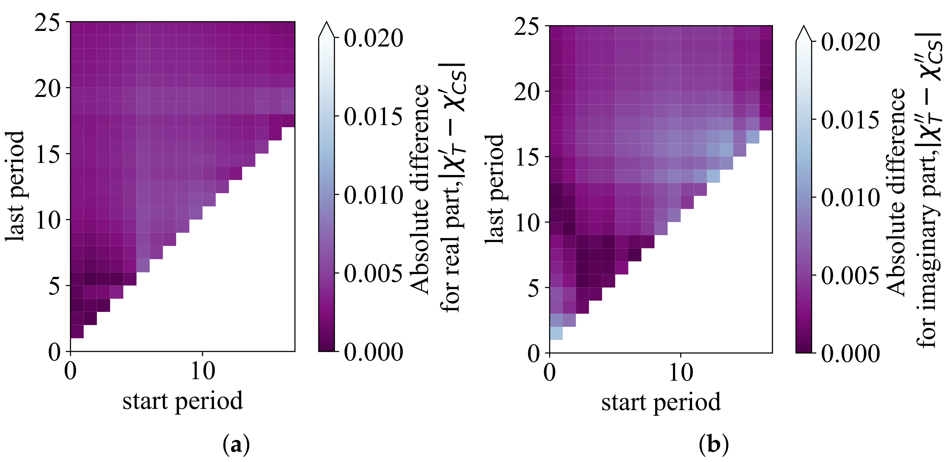
The Langevin dynamics equations should be solved until the time moment that corresponds to at least 22 periods of the AC magnetic field. Obtained dynamic magnetization should be averaged over all calculated periods, excluding at least the first four ones.

2.

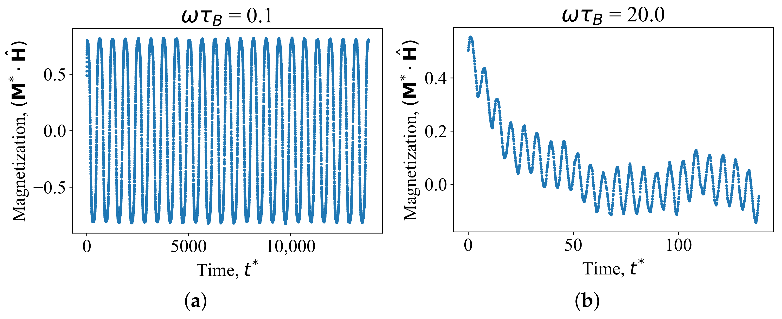
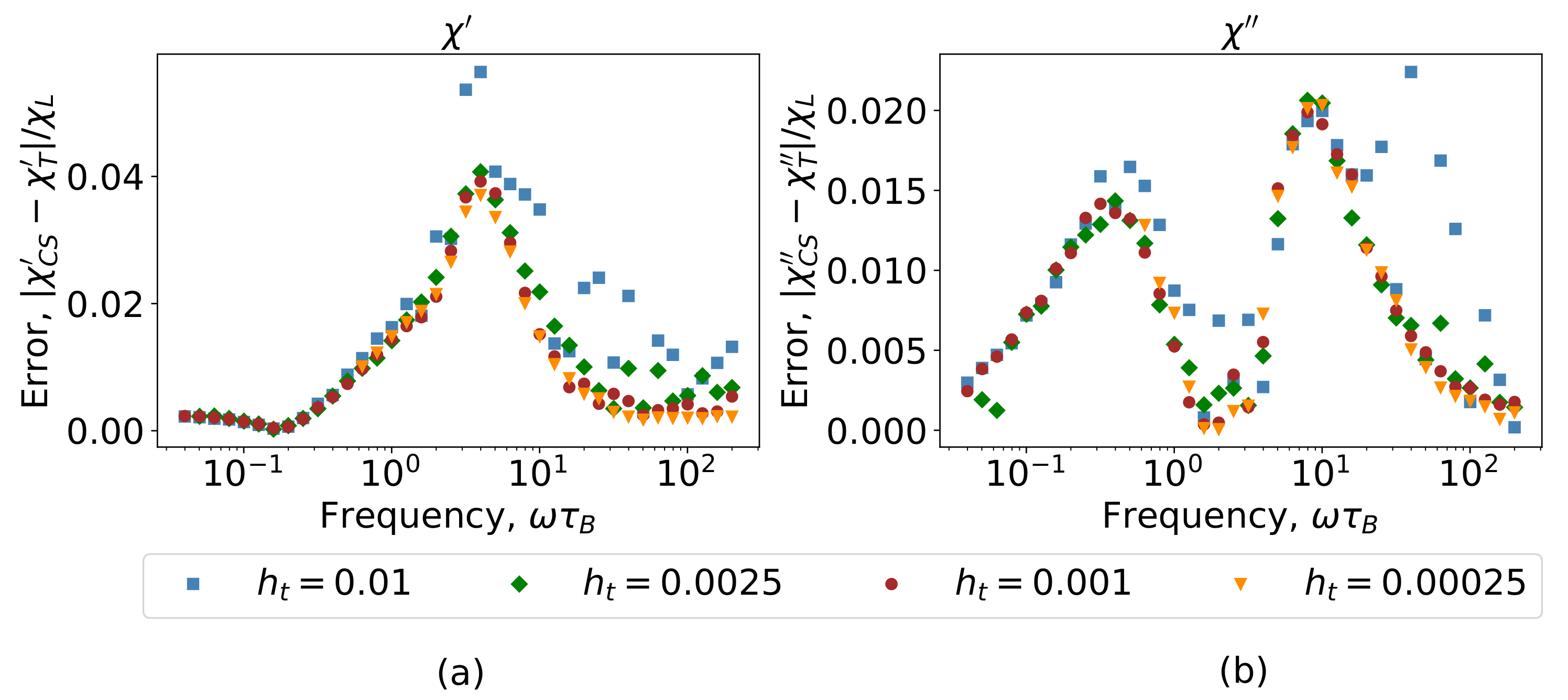
It is necessary to use different time steps in different frequency ranges: $h_t=0.0025$ if $\omega {\tau }_B\in [{10}^{-2},{10}^{-1})$, $h_t=0.001$ if $\omega {\tau }_B\in [{10}^{-1},1)$, $h_t=0.00025$ if $\omega {\tau }_B\in [1,{10}^2]$.

3.

The step size $h_{int}$ has to be the same order as $h_t$—for example, $h_{int}=5h_t$.

These recommendations with a time step decrement starting from a certain frequency were used to determine the dynamic susceptibility of an ensemble of noninteracting magnetic particles distributed in a medium with different viscosities of a carrier liquid. The viscosity is modeled by friction constant ${\Gamma }_R^{*}$ in Equations (6)–(8). The results for different friction constants are shown in Figure 7. The results for $\alpha =5$ can be found in Figure 7a; Figure 7b shows the data for $\alpha =10$. Lines correspond to the theoretical results obtained using Equation (10); symbols are chosen for the computer simulation data. Blue squares and lines correspond to the real and imaginary susceptibility for the friction constant ${\Gamma }_R^{*}=20$. For ${\Gamma }_R^{*}=40$, we used green circles and lines, and red rhombi and lines are chosen for the real and imaginary susceptibility for ${\Gamma }_R^{*}=80$. Increasing viscosity of the medium leads to a shift in the maximum of the imaginary part of the susceptibility to the low-frequency region; the value of the maximum does not depend on the medium viscosity. The plateau in the region of low frequencies of the real part of the susceptibility is longer for systems with lower viscosity. An increase of the amplitude of the AC field leads to a decrease in the values of the real and imaginary parts of the susceptibility, and hence to a decrease in the dynamic magnetic response of the system. The latter is confirmed by experimental data [39].

In Figure 8, the dynamic susceptibility of an ensemble of interacting magnetic particles is shown. Computer simulation results plotted by symbols are shown in comparison with the reference Yoshida–Enpuku theory (10) for noninteracting particles plotted by lines. Blue circles correspond to the real part of the susceptibility; orange squares are chosen for the imaginary part. Solid and dashed black lines are the real and imaginary parts of the susceptibility obtained in the reference theory correspondingly. Figure 8a contains the data for the Langevin parameter $\alpha =5$; Figure 8b is for $\alpha =10$. In Figure 8b, it is seen that the dipole–dipole interaction is suppressed by the dipole–field energy, and the susceptibilities of the interacting and noninteracting systems almost coincide. A similar behavior of the magnetic susceptibility at large amplitudes was described in the work for a system of immobilized interacting superparamagnetic particles [40]. With an increase of the amplitude of the AC field, dipole–dipole interactions begin to appear; that leads to an increase of the susceptibility, which is demonstrated in Figure 8a.

4. Conclusions

In this work, we have shown that the arising computational errors in the LD computer simulation of the dynamic susceptibility of a ferrofluid in a high-amplitude alternating magnetic field at high frequencies can be minimized by carefully adjusting the input parameters of the numerical algorithm, namely the time step $h_t$ for the solution stochastic Equations (6) and (7), the time step $h_{int}$ for calculation of integrals (9), and the number of calculation periods. Despite the fact that the exact values of input parameters depend on the system under consideration, we have given practical recommendations that make it possible to obtain reliable results of the dynamic susceptibility of a ferrofluid in an AC field of high amplitude $5\le \alpha \le 10$ in a wide frequency range, at least $\omega {\tau }_B\le {10}^{-2}$. As a criterion for assessing the reliability of the obtained computer simulation results, we chose a good agreement between the computer simulation data of dynamic susceptibility and the Yoshida–Enpuku theory (10). Recommendations are described in detail in the Results and Discussion sections and include (1) using different time steps in different frequency ranges for calculating dynamic magnetization, (2) solving the Langevin dynamics equations until the moment of time that corresponds to at least 22 periods of the external magnetic field, (3) using the averaged magnetization over all calculated periods, excluding the first few periods, and (4) increasing the integration step $h_{int}$ in comparison with the step $h_t$. All of these recommendations allow us to accumulate reliable statistics. Using these recommendations, we simulate the dynamic susceptibility of a ferrofluid with different viscosity, concentration, and intensity of interparticle dipole–dipole interactions in a wide range of amplitudes and frequencies of the AC field.

References

1. Wu, S.; Hu, W.; Ze, Q.; Sitti, M.; Zhao, R. Multifunctional magnetic soft composites: A review. Multifunct. Mater. 2020, 3, 042003. [Google Scholar] [CrossRef]
2. Menzel, A.M. Tuned, driven, and active soft matter. Phys. Rep. 2015, 554, 1–45. [Google Scholar] [CrossRef] [Green Version]
3. Arain, M.B.; Bhatti, M.M.; Zeeshan, A.; Alzahrani, F.S. Bioconvection Reiner-Rivlin Nanofluid Flow between Rotating Circular Plates with Induced Magnetic Effects, Activation Energy and Squeezing Phenomena. Mathematics 2021, 9, 2139. [Google Scholar] [CrossRef]
4. Zhang, X.; Sun, L.; Yu, Y.; Zhao, Y. Flexible Ferrofluids: Design and Applications. Adv. Mater. 2019, 31, 1903497. [Google Scholar] [CrossRef] [PubMed]
5. Pankhurst, Q.; Thanh, N.; Jones, S.; Dobson, J. Progress in applications of magnetic nanoparticles in biomedicine. J. Phys. D Appl. Phys. 2009, 42, 224001. [Google Scholar] [CrossRef] [Green Version]
6. Dutz, S.; Buske, N.; Landers, J.; Gräfe, C.; Wende, H.; Clement, J. Biocompatible magnetic fluids of co-doped iron oxide nanoparticles with tunable magnetic properties. Nanomaterials 2020, 10, 1019. [Google Scholar] [CrossRef] [PubMed]
7. Dutz, S.; Hergt, R. Magnetic nanoparticle heating and heat transfer on a microscale: Basic principles, realities and physical limitations of hyperthermia for tumour therapy. Int. J. Hyperth. 2013, 29, 790–800. [Google Scholar] [CrossRef] [PubMed]
8. Gopika, M.; Lahiri, B.; Anju, B.; Philip, J.; Savitha Pillai, S. Magnetic hyperthermia studies in magnetite ferrofluids based on bio-friendly oils extracted from Calophyllum inophyllum, Brassica juncea, Ricinus communis and Madhuca longifolia. J. Magn. Magn. Mater. 2021, 537, 168134. [Google Scholar] [CrossRef]
9. Lahiri, B.; Ranoo, S.; Muthukumaran, T.; Philip, J. Magnetic hyperthermia in water based ferrofluids: Effects of initial susceptibility and size polydispersity on heating efficiency. AIP Conf. Proc. 2018, 1942, 040019. [Google Scholar]
10. Gleich, B.; Weizenecker, J. Tomographic imaging using the nonlinear response of magnetic particles. Nature 2005, 435, 1214–1217. [Google Scholar] [CrossRef]
11. Dieckhoff, J.; Kaul, M.; Mummert, T.; Jung, C.; Salamon, J.; Adam, G.; Knopp, T.; Ludwig, F.; Balceris, C.; Ittrich, H. In vivo liver visualizations with magnetic particle imaging based on the calibration measurement approach. Phys. Med. Biol. 2017, 62, 3470–3482. [Google Scholar] [CrossRef]
12. Salamon, J.; Dieckhoff, J.; Kaul, M.; Jung, C.; Adam, G.; Möddel, M.; Knopp, T.; Draack, S.; Ludwig, F.; Ittrich, H. Visualization of spatial and temporal temperature distributions with magnetic particle imaging for liver tumor ablation therapy. Sci. Rep. 2020, 10, 7480. [Google Scholar] [CrossRef] [PubMed]
13. Raikher, Y.L.; Shliomis, M.I. The effective field method in the orientational kinetics of magnetic fluids. Adv. Chem. Phys. 1994, 87, 595–751. [Google Scholar]
14. Fock, J.; Balceris, C.; Costo, R.; Zeng, L.; Ludwig, F.; Hansen, M. Field-dependent dynamic responses from dilute magnetic nanoparticle dispersions. Nanoscale 2018, 10, 2052–2066. [Google Scholar] [CrossRef] [Green Version]
15. Debye, P. Polar Molecules; Chemical Catalog Company: New York, NY, USA, 1929. [Google Scholar]
16. Fröhlich, H. Theory of Dielectrics: Dielectric Constant and Dielectric Loss; Clarendon Press: Oxford, UK, 1987. [Google Scholar]
17. Yoshida, T.; Enpuku, K. Simulation and quantitative clarification of AC susceptibility of magnetic fluid in nonlinear Brownian relaxation region. Jpn. J. Appl. Phys. 2009, 48, 127002. [Google Scholar] [CrossRef]
18. Coffey, W.T.; Kalmykov, Y.P.; Wei, N. Nonlinear normal and anomalous response of non-interacting electric and magnetic dipoles subjected to strong AC and DC bias fields. Nonlinear Dyn. 2015, 80, 1861–1867. [Google Scholar] [CrossRef]
19. Raikher, Y.; Stepanov, V. Power losses in a suspension of magnetic dipoles under a rotating field. Phys. Rev. E 2011, 83, 021401. [Google Scholar] [CrossRef]
20. Djardin, P.; Kalmykov, Y.; Kashevsky, B.; El Mrabti, H.; Poperechny, I.; Raikher, Y.; Titov, S. Effect of a dc bias field on the dynamic hysteresis of single-domain ferromagnetic particles. J. Appl. Phys. 2010, 107, 073914. [Google Scholar] [CrossRef]
21. Batrudinov, T.; Ambarov, A.; Elfimova, E.; Zverev, V.; Ivanov, A. Theoretical study of the dynamic magnetic response of ferrofluid to static and alternating magnetic fields. J. Magn. Magn. Mater. 2017, 431, 180–183. [Google Scholar] [CrossRef]
22. Lebedev, A.; Stepanov, V.; Kuznetsov, A.; Ivanov, A.; Pshenichnikov, A. Dynamic susceptibility of a concentrated ferrofluid: The role of interparticle interactions. Phys. Rev. E 2019, 100, 032605. [Google Scholar] [CrossRef]
23. Lebedev, A.; Kantorovich, S.; Ivanov, A.; Arefyev, I.; Pshenichnikov, A. Weakening of magnetic response experimentally observed for ferrofluids with strongly interacting magnetic nanoparticles. J. Mol. Liq. 2019, 277, 762–768. [Google Scholar] [CrossRef]
24. Ivanov, A.O.; Zverev, V.S.; Kantorovich, S.S. Revealing the signature of dipolar interactions in dynamic spectra of polydisperse magnetic nanoparticles. Soft Matter 2016, 12, 3507–3513. [Google Scholar] [CrossRef] [PubMed] [Green Version]
25. Ivanov, A.; Camp, P. Theory of the dynamic magnetic susceptibility of ferrofluids. Phys. Rev. E 2018, 98, 050602. [Google Scholar] [CrossRef] [Green Version]
26. Berkov, D.V.; Iskakova, L.Y.; Zubarev, A.Y. Theoretical study of the magnetization dynamics of nondilute ferrofluids. Phys. Rev. E 2009, 79, 021407. [Google Scholar] [CrossRef] [PubMed] [Green Version]
27. Rusanov, M.; Zverev, V.; Elfimova, E. Dynamic magnetic susceptibility of a ferrofuid: The influence of interparticle interactions and AC field amplitude. Phys. Rev. E 2021, 104, 044604. [Google Scholar] [CrossRef]
28. Hansen, J.; McDonald, I. Theory of Simple Liquids, 3rd ed.; Academic Press: Burlington, MA, USA, 2006. [Google Scholar]
29. Batrudinov, T.; Nekhoroshkova, Y.; Paramonov, E.; Zverev, V.; Elfimova, E.; Ivanov, A.; Camp, P. Dynamic magnetic response of a ferrofluid in a static uniform magnetic field. Phys. Rev. E 2018, 98, 052602. [Google Scholar] [CrossRef] [Green Version]
30. Sindt, J.O.; Camp, P.J.; Kantorovich, S.S.; Elfimova, E.A.; Ivanov, A.O. Influence of dipolar interactions on the magnetic susceptibility spectra of ferrofluids. Phys. Rev. E 2016, 93, 063117. [Google Scholar] [CrossRef] [Green Version]
31. Allen, M.P.; Tildesley, D.J. Computer Simulation of Liquids; Clarendon Press: Oxford, UK, 1987. [Google Scholar]
32. Tuckerman, M.; Berne, B.J.; Martyna, G.J. Reversible multiple time scale molecular dynamics. J. Chem. Phys. 1992, 97, 1990–2001. [Google Scholar] [CrossRef] [Green Version]
33. Omelyan, I. Numerical integration of the equations of motion for rigid polyatomics: The matrix method. Comput. Phys. Commun. 1998, 109, 171–183. [Google Scholar] [CrossRef] [Green Version]
34. Martys, N.S.; Mountain, R.D. Velocity Verlet algorithm for dissipative-particle-dynamics-based models of suspensions. Phys. Rev. E 1999, 59, 3733–3736. [Google Scholar] [CrossRef]
35. Weik, F.; Weeber, R.; Szuttor, K.; Breitsprecher, K.; de Graaf, J.; Kuron, M.; Landsgesell, J.; Menke, H.; Sean, D.; Holm, C. ESPResSo 4.0—An extensible software package for simulating soft matter systems. Eur. Phys. J. Spec. Top. 2019, 227, 1789–1816. [Google Scholar] [CrossRef] [Green Version]
36. Cerda, J.J.; Ballenegger, V.; Lenz, O.; Holm, C. P3M algorithm for dipolar interactions. J. Chem. Phys. 2008, 129, 234104. [Google Scholar] [CrossRef] [PubMed] [Green Version]
37. Brown, J.W.F. Thermal Fluctuations of a Single-Domain Particle. Phys. Rev. 1963, 130, 1677–1686. [Google Scholar] [CrossRef]
38. Kalambet, Y.; Kozmin, Y.; Samokhin, A. Comparison of integration rules in the case of very narrow chromatographic peaks. Chemom. Intell. Lab. Syst. 2018, 179, 22–30. [Google Scholar] [CrossRef]
39. Dieckhoff, J.; Eberbeck, D.; Schilling, M.; Ludwig, F. Magnetic-field dependence of Brownian and Néel relaxation times. J. Appl. Phys. 2016, 119, 043903. [Google Scholar] [CrossRef]
40. Ambarov, A.V.; Zverev, V.S.; Elfimova, E.A. Numerical modeling of the magnetic response of interacting superparamagnetic particles to an ac field with arbitrary amplitude. Model. Simul. Mater. Sci. Eng. 2020, 28, 085009. [Google Scholar] [CrossRef]
Figure 1. Dynamic magnetization of noninteracting magnetic particles under AC field with the amplitude α = 5 . The rotational friction constant is Γ R * = 40 , and the AC field angular frequencies ω τ B are: (a)— ω τ B = 0.1 ; (b)— ω τ B = 20.0 . Each magnetization curve contains 22 periods of the AC field.
Mathematics 09 02581 g001
Figure 2. Absolute difference between theoretical χ T and computer simulation χ C S data of the (a) real and (b) imaginary parts of the dynamic susceptibility at the AC field angular frequency ω τ B = 20.0 for the system with α = 5 , Γ R * = 40 in dependence on the number of computational periods. The last period shows the number of periods of the AC field over which the averaging of the magnetization was carried out for calculating the susceptibility; the start period is the number of the first periods of the calculation, which are omitted during averaging. Computer simulations were performed with the time step h t = 0.00025 . Theoretical values of the dynamic susceptibility were calculated from Equation (10): χ T ( ω τ B ) = 0.004 , χ T ( ω τ B ) = 0.055 .
Mathematics 09 02581 g002
Figure 3. Dynamic susceptibility χ / χ L as a function of a reduced field frequency ω τ B for AC field amplitudes (a) α = 5 and (b) α = 10 . Lines are from the Yoshida–Enpuku theory [17] (Equation (10)), symbols are computer simulation results. Computer simulations were performed with time steps h t = 0.01 , h t = 0.0025 , h t = 0.001 and h t = 0.00025 .
Mathematics 09 02581 g003
Figure 4. Difference between theoretical χ T and computer simulation χ C S data of the (a) real and (b) imaginary parts of the dynamic susceptibility from the Figure 3b for the AC field amplitude α = 10 . Different colors and shapes of symbols correspond to different time steps h t = 0.01 , h t = 0.0025 , h t = 0.001 , and h t = 0.00025 .
Mathematics 09 02581 g004
Figure 5. Dynamic susceptibility χ / χ L as a function of a reduced field frequency ω τ B for AC field amplitudes (a) α = 5 and (b) α = 10 . Lines are from the Yoshida–Enpuku theory (10); symbols are computer simulation results. The integral (9) is calculated by different time steps h i n t = 0.1 (blue squares) and h i n t = 0.005 (green circles); h t = 0.001 .
Mathematics 09 02581 g005
Figure 6. The modulus of the difference between the (a) real and (b) imaginary parts of the susceptibility calculated from LD simulations for different time steps h 1 and h 2 : (a) Δ χ ( h 1 , h 2 ) = χ ( h 1 ) χ ( h 2 ) , (b) Δ χ ( h 1 , h 2 ) = χ ( h 1 ) χ ( h 2 ) . The absolute deviation is shown by horizontal dashed lines. Susceptibility values correspond to the system from Figure 3b, h i n t , i = 5 h i , i { 1 , 2 } .
Mathematics 09 02581 g006
Figure 7. Dynamic susceptibility χ / χ L of noninteracting magnetic particles distributed in a medium with different viscosities of a carrier liquid as a function of a field frequency ω t 0 for AC field amplitude (a) α = 5 and (b) α = 10 . Symbols correspond to the computer simulation data; lines are chosen for theoretical results (Equation (10)). Filled symbols and solid lines are the real part of the susceptibility; unfilled symbols and dashed lines are the results for its imaginary part. Different colors and shapes of symbols are chosen for different friction constants Γ R * .
Mathematics 09 02581 g007
Figure 8. Dynamic susceptibility χ / χ L as a function of a field frequency ω τ B for the AC field amplitude (a) α = 5 and (b) α = 10 obtained for the friction constant Γ R * = 80 . Lines correspond to the Yoshida–Enpuku theory (10) for noninteracting particles; symbols are the computer simulation data for interacting particles with χ L = 1 .
Mathematics 09 02581 g008
Publisher’s Note: MDPI stays neutral with regard to jurisdictional claims in published maps and institutional affiliations.