An Empirical Equation for Failure Pressure Prediction of High Toughness Pipeline with Interacting Corrosion Defects Subjected to Combined Loadings Based on Artificial Neural Network

Abstract

Conventional pipeline corrosion assessment methods for failure pressure prediction do not account for interacting defects subjected to internal pressure and axial compressive stress. In any case, the failure pressure predictions are conservative. As such, numerical methods are required. This paper proposes an alternative to the computationally expensive numerical methods, specifically an empirical equation based on Finite Element Analysis (FEA). FEA was conducted to generate training data for an ANN after validating the method against full scale burst test results from past research. An ANN with four inputs and one output was developed. The equation was developed based on the weights and biases of an ANN model trained with failure pressure from the FEA of a high toughness pipeline for various defect spacings, defect depths, defect lengths, and axial compressive stresses. The proposed model was validated against actual burst test results for high toughness materials, with a R² value of 0.99. Extensive parametric study was subsequently conducted to determine the effects of defect spacing, defect length, defect depth, and axial compressive stress on the failure pressure of the pipe. The results of the empirical equation are comparable to the results from numerical methods for the pipes and loadings considered in this study.

1. Introduction

1.1. Overview of Pipelines in the Oil and Gas Industry

Pipelines are widely utilized for upstream oil and gas operations for the transportation of hydrocarbon from the reservoir to onshore processing facilities. On average, a pipeline stretches across hundreds of kilometers, operating at high pressures and temperatures. This harsh environment results in pipe wall degradation, also known as corrosion [1]. In a pristine pipe, the hoop stress is distributed evenly throughout the pipe. However, in the presence of corrosion defects, the hoop stress distribution is nonuniform [2,3,4].

When fluid flows through a pipeline, internal pressure is exerted on the pipe wall causing circumferential expansion which results in the contraction of the pipe in the longitudinal direction due to Poisson’s effect [5,6,7]. This condition subjects the pipeline to axial compressive stress. Strain builds up at the region of defect, making it the most critical region in the pipeline [8,9]. In the region of defect, the deepest defect experiences the highest stress. When the stress exceeds the true ultimate tensile strength of the pipe, the pipe fails prematurely. The failure pressure of a pipeline is significantly influenced by the length and depth of the corrosion defect when subjected to axial compressive stress [10,11,12], especially in the presence of interacting defects. It is therefore crucial that the integrity of a pipeline is assessed periodically to ensure a safe and efficient operation.

1.2. Pipeline Integrity Assessment Methods

Developing a corrosion assessment method that is applicable for all types of corrosion defects as well as pipeline grades is challenging due to the complexity of the corrosion defect geometry and differences in tensile properties of materials [13,14,15,16,17]. As such, different assessment methods are used for different scenarios. Furthermore, various assumptions are made to simplify the assessment. As such, the failure pressure prediction of a pipe for each corrosion assessment method differs due to these simplifications.

By redefining the Folias factor and flow stress equations of the ASME B31G method, the Modified ASME B31G method was developed. In this method, an arbitrary shape correction factor is applied instead of the parabolic area assumption. This enables the method to be applied to corrosion defects that are longer than the limits given in the ASME B31G method. The SHELL 92 method also utilizes the same Folias factor as the ASME B31G method. However, this method produces predictions that are relatively conservative due to the flow stress assumption of the method [16].

The RSTRENG method, also known as the effective area method, is used in assessing defects up to 0.8 t. This method represents the corrosion defect region with a river bottom profile that enables failure pressure prediction with greater accuracy using the discrete method [16,18]. The Pipe Corrosion Criterion (PCORRC) method is based on a finite element study that was validated using burst test results.

The ASME B31G, Modified B31G, SHELL 92, and RSTRENG methods were developed based on the NG-18 as the fundamental equation. In these methods, it is assumed that the tensile property of a pipe material determines the pipe failure mechanism [2,14,15]. However, the governing assumption of the DNV-RP-F101 code, which was also developed based on the NG-18 equation, is that the failure of the pipe is due to plastic collapse (plastic flow), where the ultimate tensile strength is the flow stress. This governing assumption is also applied to the PCORRC method that was developed based on numerical studies. In all these methods, the corrosion depth and longitudinal length are considered and are independent of the width of the corrosion. The conservatism in these methods due to the assumptions, simplifications, and safety factor leads to unwarranted repairs and premature replacement of a pipeline, incurring unnecessary costs [9,19].

For pipes subjected to internal pressure and axial compressive stress, the DNV corrosion assessment code is the most comprehensive code [2]. The DNV code allows for failure pressure prediction of single and interacting corrosion defects subjected to internal pressure only, and single defects subjected to internal pressure and axial compressive stress [15]. The DNV code has been compared against actual full scale burst pressure tests for medium toughness pipes with material grades ranging from API 5L X42 to API 5L X65. Nevertheless, the failure pressure predictions based on this code are conservative. This conservatism is primarily due to the use of the ultimate tensile strength, σ_UTS, rather than the true ultimate tensile strength, σ×_UTS, of the material [9], since the rupture point of a material is represented by the true ultimate tensile strength of the material [2].

As this method is developed for medium toughness pipes, utilizing it for high toughness pipes may result in inaccurate failure pressure predictions [9]. Hence, an alternative failure pressure prediction method is necessary to overcome the limitations of this failure pressure assessment method, which are summarized in the points below:

• The DNV code does not incorporate axial compressive stress for the failure pressure assessment of interacting corrosion defects.
• The DNV code results in conservative failure pressure predictions.
• The DNV code results in inaccurate failure pressure predictions for high toughness pipes.

1.3. Finite Element Method (FEM) for Pipeline Failure Pressure Prediction

Due to the limitations of the assessment codes, numerical methods are utilized. The American Society of Mechanical Engineers categorized numerical methods such as FEM as a Level 3 assessment method, which is considered to be the most advanced assessment level [14]. FEM considers the uniaxial true stress-strain curve of a material, important for structures that change in geometry due to large displacements. As the pipe undergoes deformation, the equilibrium equations take into consideration the geometrical changes of the pipe as well as the nonlinear stress-strain relationship of the material. Strain hardening as well as elastic and plastic deformation of the material is accounted for in the assessment process, resulting in good failure pressure prediction [3].

The complex geometries of corrosion defects are often idealized as simple shapes in FEM for ease of assessment. The most common idealized defect shapes are rectangular, elliptical, parabolic, and in some cases conical shape [19,20,21,22]. Wang et al. [23] investigated the failure pressure difference between finite element models with rectangular defect and elliptical defect. The study found that there is an insignificant difference in failure pressure prediction between the two idealized defects. Conventional standards, such as the DNV code, commonly idealize corrosion defects as rectangular-shaped defects [13,15,24].

However, the accuracy of the failure pressures obtained using FEM is highly dependent on the proper choice of boundary conditions, material properties, and model features [21]. The meshing size of the model also plays an important role in the accuracy of the results. Smaller meshes result in high accuracy but consume longer simulation time. Hence, the modeling of the pipe has to be optimized to reduce simulation time without compromising the accuracy of the results [25]. The FEM results will be erroneous if any of the components are poorly defined, resulting in wrong failure pressure predictions. Hence, the FEM needs to be validated against actual burst test. This process can be very time consuming, especially when it involves the incorporation of axial compressive stress.

Even if the FEM is correct, it is computationally expensive. Many researchers apply the eXtended Finite Element Method (XFEM) in their studies to overcome the limitations of FEM in the field of fracture mechanics. Since damage mechanics is mesh dependent, XFEM allows pipeline failure prediction under various loading conditions without refining the mesh closer to the region of interest [26]. Using this approach, the mesh conformance of crack geometry is avoided [27]. Okodi et al. investigated the potential of XFEM to be used in crack propagation analysis and burst pressure prediction of pipelines [28]. It was found that XFEM can be effective in carrying out crack propagation analysis, as well as predicting pipeline burst pressure, but it was recommended that further parametric studies be done to come to a firm conclusion. Their study was further supported by Zhang et al., who investigated the failure pressure prediction of cracks in corrosion defects [29]. It was concluded that XFEM is useful for crack propagation analysis, whereby if FEM was applied, it would require extremely fine meshes. Hence, XFEM is suitable for problems with interior boundaries, discontinuities, or singularities because of the need of remeshing and high mesh densities [30]. In predicting the failure pressure of corroded pipelines using a stress-based von Mises criterion, the entire surface of the model coincides with the edge of the FEA [2,9,31,32]. In such cases, FEM is adequate [30].

FEM is widely utilized to analyze the stress distribution across pipes and identify the pressure at which the point of failure occurs for corroded pipelines. Colindres et al. investigated the effects of internal and external corrosion defects using the stress-based von Mises criterion using FEM. In their paper, they recommended FEM be utilized for complex corrosion defect cases in pipelines [31]. To reduce the computation time, quarter models are usually utilized with symmetric boundary conditions that treat the pipe as a whole during simulation. Despite this, a single simulation run can take hours to complete. As such, using FEM for the failure pressure prediction of multiple corroded pipelines subjected to internal pressure and axial compressive stress is not practical, especially in time critical situations.

To overcome this, a simple empirical solution with wide applicability, as an alternative to the DNV-RP-F101 equations, that is as accurate as a Level 3 assessment method is proposed. However, there is a nonlinear relationship between the geometry of a defect and axial compressive stress with the failure pressure of the corroded pipe [9]. The defect length, defect depth, and amount of axial compressive stress imposed on the pipe can occur in various combinations. As such, it is not trivial to develop the empirical equation, as large data will be required to analyze this nonlinear relationship. As such, this nonlinearity can be analyzed using FEM simulation and the data could be used to validate the equation [32].

An empirical equation, based on the weights and biases of an ANN trained using results from FEA, can be used to provide failure pressure predictions within seconds. Xu et al. [33] utilized FEA to generate training data for the development of an ANN to predict the failure pressure of a corroded pipe with a relative error percentage of less than 1%. A parametric study was conducted, and the data were used to train an ANN. There was an insignificant error between the experimental values and results obtained from the trained ANN. This approach was also followed by Lu and Liang [34], and Gholami et al. [35], who studied the effects of defect geometry on the failure pressure of a corroded pipe using FEM and used the data to train an ANN model. As such, FEM is a reliable method for obtaining training data for the development of an ANN. Based on the weights and biases of the trained ANN, an empirical equation can be developed with ease.

1.4. Artificial Neural Network (ANN) as a Pipeline Failure Pressure Assessment Method

Gurney [36] defined an ANN as an interconnected assembly of simple processing elements called nodes and the processing ability of the network is stored in the interunit connection strengths called weights which are obtained by learning a set of training patterns. A neural network mimics the synapses in a human brain by employing weights and biases to neurons in hidden layers of the neural network and reinitializes them until the neural network produces accurate results [37]. When this is achieved, the neural network is said to be trained. It is crucial that the training dataset consists of a sufficient number of inputs and corresponding outputs to minimize the error in the output of the neural network [38,39,40].

An ANN has the ability to learn, recognize, and infer from complex nonlinear data without requiring an explicit set of instruction [40,41]. A set of data that consists of one or more inputs and outputs is analyzed by the neural network using specific algorithms depending on the ANN type and purpose. An ANN is capable of learning directly from a set of training data, and regaining as well as extracting information from noisy data is one of the most important properties of it that has been proven to be very useful in the field of mechanical failure analysis [41].

Various studies on fracture toughness and fracture parameters utilizing ANN have been carried out by many researchers and this approach has shown promising results. A trained ANN was able to produce results that were very close to the training data fed to the ANN with an acceptable accuracy [41]. Furthermore, an ANN does not require simplifications or assumptions to process and learn from the training data. Moreover, the study conducted by Ince [42] to predict the fracture parameters of concrete using ANN proved that ANNs can also be utilized to carry out parametric studies.

The architecture of an ANN also depends on the type of data and desired output. Among the commonly used ANN architectures, a Feed Forward Neural Network (FFNN) is mostly utilized in predicting the failure pressure of corroded pipelines. This type of neural network paired with back propagation supervised learning algorithm is typically utilized as it examines the training data and generates an inferred function that can be applied to new scenarios [43,44,45]. This type of ANN architecture is modeled to learn from paired datasets where the model learns from one or more inputs and the corresponding output of the training dataset.

The utilization of ANN in the field of failure pressure assessment has improved over the years, resulting in more practical applications. In early applications of ANN, researchers took into account the physical, mechanical, operational, and environmental factors that influenced the residual strength of a pipeline [46]. However, obtaining a large training dataset for such cases is challenging. Shirzad et al. [47] and Senouci et al. [48] emphasized in their paper that an ANN model with a reasonable accuracy and robustness cannot be achieved with the lack of real-life data. Xu et al. conducted parametric studies using FEM to generate a training dataset for an ANN model to accurately predict the failure pressure of a high toughness pipe with a relative error of less than 2% [33]. Their results were supported by Lu and Liang [34] and Gholami et al. [35], who developed an ANN model based on data generated from FEA. It was proven that an ANN is highly capable of predicting the failure pressure of a corroded pipeline accurately.

This study aims to establish a correlation between defect geometries and failure pressure of high toughness corroded pipelines and develop an empirical corrosion assessment method for the failure prediction of high toughness corroded pipelines subjected to internal pressure and axial compressive stress. The empirical equation was developed based on the weights and biases of an ANN trained with values from parametric studies utilizing FEA. The equation was then validated against FE models with single defect corrosion and full-scale burst tests.

2. Methodology

2.1. Overview of Geometric Parameters, Assessment Factors, and Assumptions

In this study, four parameters, the defect length, defect depth, defect spacing, and axial compressive stress, were considered for the prediction of failure pressure of a pipe with interacting corrosion defects, with the defect width kept constant. These parameters are represented as normalized values. For the pipe model, a diameter of 300 mm, wall thickness of 10 mm, and length of 2000 mm were utilized. The corrosion defect geometry is represented as normalized values as listed in

Table 1. Corrosion defect geometry parameters.

Corrosion Defect Geometry	Value(s)
Normalized defect width, $w/t$	10
Normalized defect spacing, $s/\sqrt{Dt}$	0.0, 0.5, 1.0, 2.0
Normalized defect depth, $d/t$	0.0, 0.2, 0.4, 0.6, 0.8
Normalized defect length, $l/D$	0.0, 0.2, 0.4, 0.6, 0.8
Normalized axial compressive stress, σc/σy	0.0, 0.2, 0.4, 0.6, 0.8

. The output of the FEA is the failure pressure of the corroded pipe.

A calibrated safety factor approach (Part A) from the DNV-RP-F101 corroded pipeline assessment manual was used for the calculation of the failure pressure of pipes with interacting defect subjected to internal pressure and axial compressive stress. In this approach, the size of the defect depth and material properties must be specified [7]. The model prediction partial safety factor, ${\gamma }_m$, corrosion depth partial safety factor, ${\gamma }_d$, and usage factor, $\xi$, was set to 1.00 to represent a perfect pipe inspection method, exact corrosion defect depth, and a pristine pipe, respectively. The fractile value, ${\epsilon }_d$, and relative depth accuracy, acc_rel, was set to 0.00 to represent low tolerance and high confidence level corrosion inspection method, and high corrosion depth inspection accuracy with zero tolerance, respectively. The confidence level, conf, was set to 0.99 to represent 99% confidence level on corrosion defect dimensions.

2.2. Development of the Finite Element Method

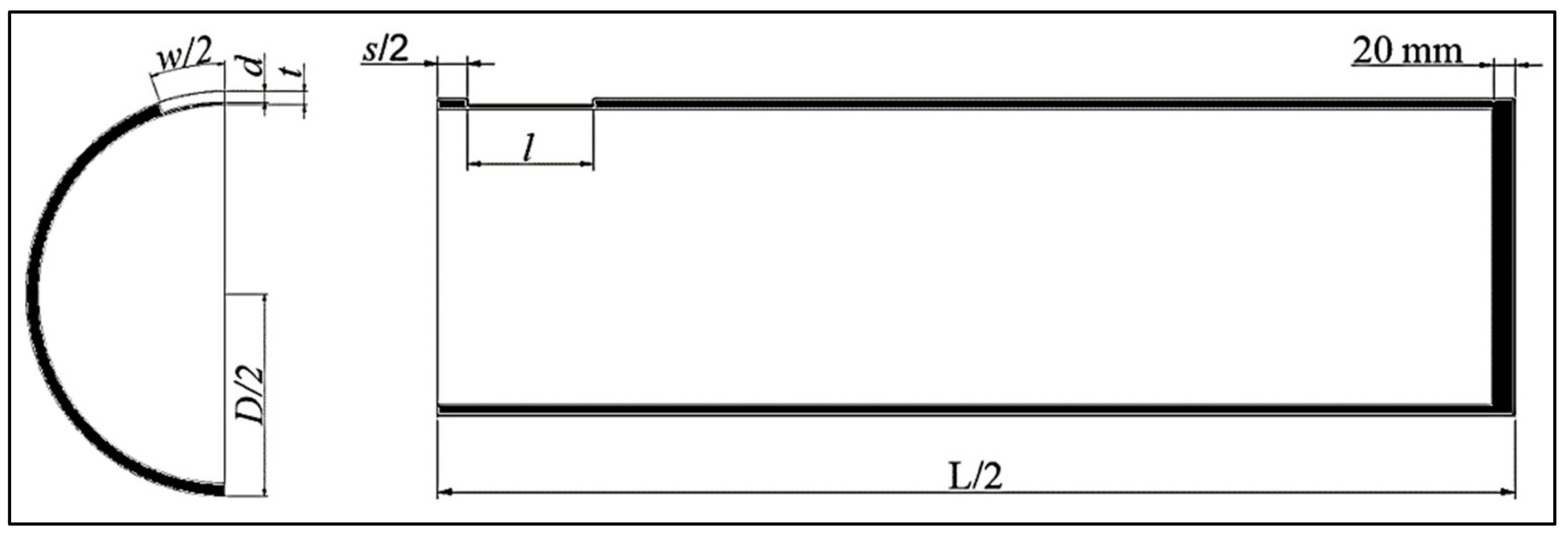
In this study, quarter models of the corroded pipes were used to reduce computation time during FEA, without compromising the accuracy of the results, as illustrated in Figure 1. The full length of the modeled pipe was set to 2000 mm to prevent end cap effects, while the pipe external diameter and wall thickness were set to be 300 mm and 10 mm, respectively. The pipes were modeled with endplates of 20 mm to ensure an even distribution of axial compressive stress across the pipe wall. A pair of rectangular-shaped corrosion defects, as utilized in the DNV method, was employed as it allows for a safer lower bound failure pressure prediction without compromising the accuracy [15,49,50,51,52].

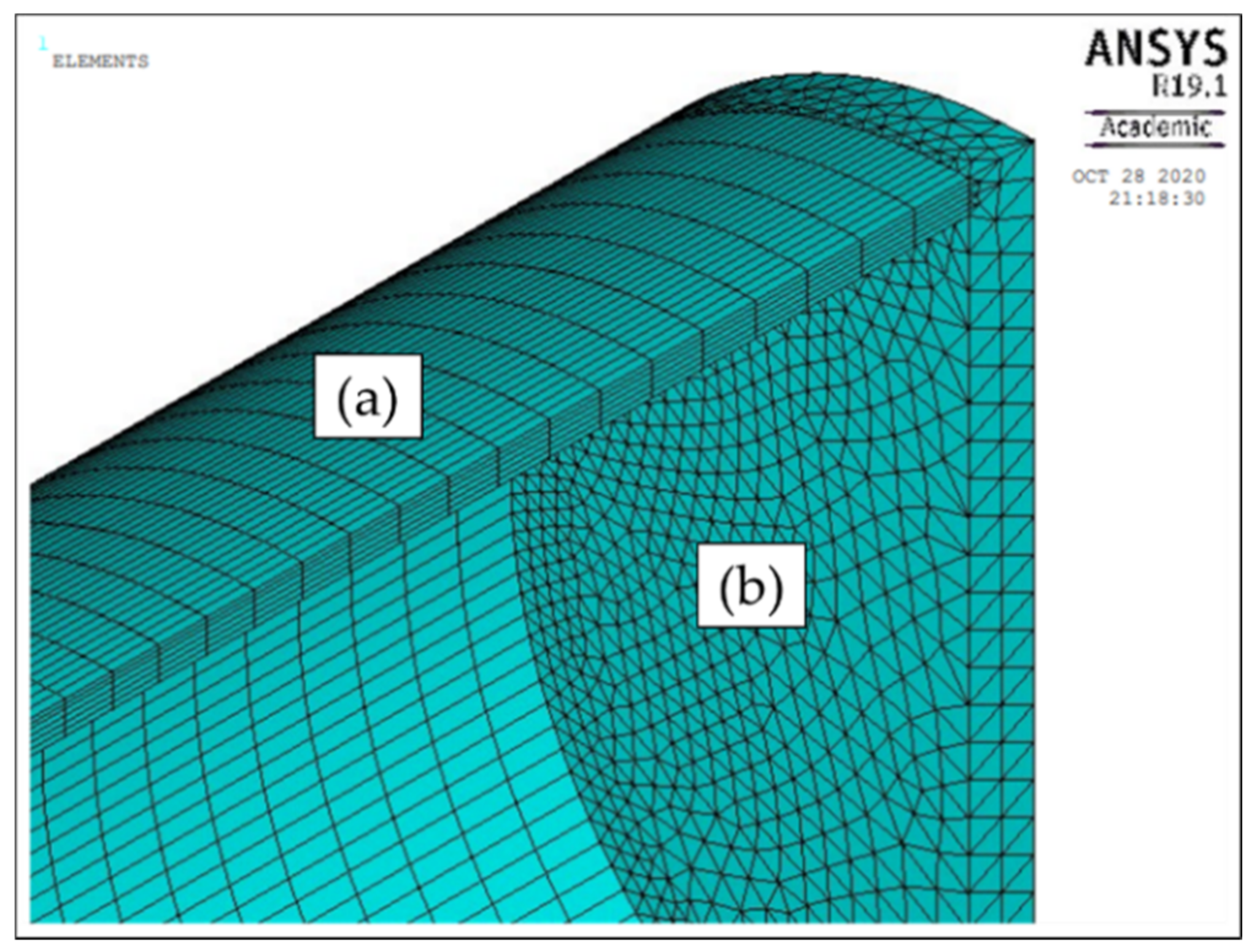
Solid elements were used for the meshing of the model instead of shell elements due to the thickness of the pipe wall, as solid elements represent the solid structure throughout, while shell elements are used to represent the outer surface of the object [23]. Hexahedral SOLID185 elements were used for the meshing of the pipe body and defect region, while tetrahedral SOLID186 elements were used for the rigid body. SOLID185 is defined by 8 nodes having three degrees of freedom while SOLID186 can tolerate irregular shapes such as curved boundaries. Both these elements cater for high stress stiffening, creep, large deflection, plasticity, swelling, and large strain [52]. The application of SOLID185 and SOLID186 elements on a pipe model is illustrated in Figure 2.

A convergence test was conducted to determine the number of layers for the meshing of the pipe model, as tabulated in

Table 2. Convergence test results for the optimum number of mesh layers at the defect region.

Number of Element Layers	$\mathbf{Normalized}\mathbf{Failure}\mathbf{Pressure},{\mathit{P}}_{\mathit{f}}/{\mathit{P}}_{\mathit{i}}$
1	0.92
2	0.93
3	0.95
4	0.95
5	0.95

. The number of layers at the defect region was set to be 3 while the length and depth of the mesh were set to be 2 mm, in line with the British Standards Institution (BSI) guidelines [53]. An aspect ratio of 0.5 was applied to the elements moving away from the defect region, with a total of 80 divisions. Before finalizing these mesh settings, a convergence test was conducted to ensure optimum computation time without compromising the accuracy of the FEM.

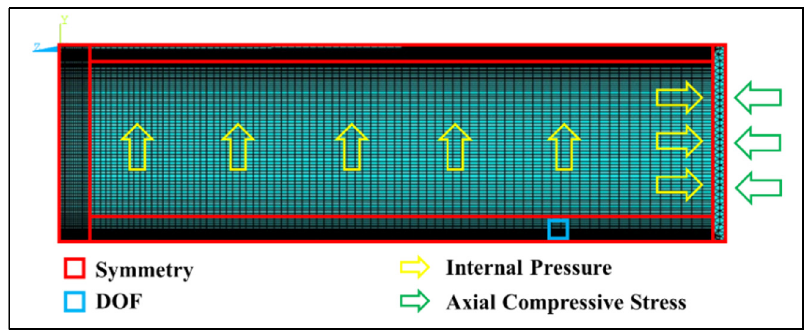
During FE simulations, appropriate boundary conditions were applied to ensure that the quarter model is treated as a whole model. Symmetric boundary conditions were imposed on each quarter model, as illustrated in Figure 3. To avoid unwanted rigid body movements, degree of freedom (DOF) constraints were applied in the x, y, and z directions at 4/5 of the quarter model length away from the region of interest (Figure 3). Internal pressure and axial compressive stress were applied using incremental ramped loading on the inner surface of the pipe and the outer surface of the rigid body, respectively (Figure 3).

The failure pressures were obtained by employing a series of linear steps to obtain an exact solution using the Newton–Raphson method. This method involves an iterative process to achieve convergence for a nonlinear problem. Initially, a solution is assumed, then the magnitude of the increment is determined. The trial solution is updated after every iteration based on the determined increment value and the iteration is repeated until convergence is achieved. A tolerance is set to terminate the solution procedure when the convergence criterion is satisfied [3].

The internal pressure and axial compressive stress were applied using incremental ramped loading on the inner surface of the pipe and the outer surface of the rigid body, respectively (Figure 3) using transient analysis. These loads were controlled using timesteps. For pipes subjected to internal pressure only, the internal pressure was applied incrementally throughout the timestep, as illustrated by Figure 4. As for pipes subjected to internal pressure and axial compressive stress, axial compressive stress was applied during the first timestep and in the second timestep, the pipe was subjected to internal pressure, as illustrated in Figure 5.

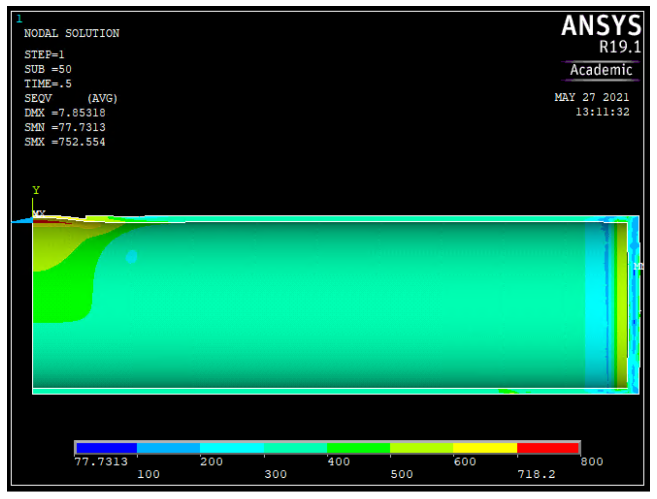
To determine the point of pipe failure, a stress-based criterion known as von Mises theory was used to analyze the stress distribution across the pipe during FEA. The material is said to have failed when the von Mises stress reaches the true ultimate tensile strength, $\sigma {\times }_{UTS}$, of the material [54]. This scenario is illustrated in Figure 6, where it can be observed that the region of defect is the most critical part of the pipe. The red region represents the area at which the von Mises stress exceeds the $\sigma {\times }_{UTS}$ of the material.

The von Mises theory that was used to analyze the effective stress, ${\sigma }_e$, is a function of hoop, ${\sigma }_h$, radial, ${\sigma }_r$, and axial stress, ${\sigma }_l$, as shown in Equation (1) [2]. When the effective stress reaches the true ultimate tensile strength of the material, the time step of the simulation is recorded and the corresponding pressure is calculated and recorded as the failure pressure of the pipe.

$${\sigma }_e=\sqrt{\frac{1}{2}\left[{\left({\sigma }_h-{\sigma }_r\right)}^2+{\left({\sigma }_h-{\sigma }_l\right)}^2+{\left({\sigma }_r-{\sigma }_l\right)}^2\right]}$$

(1)

2.3. Development of the Artificial Neural Network

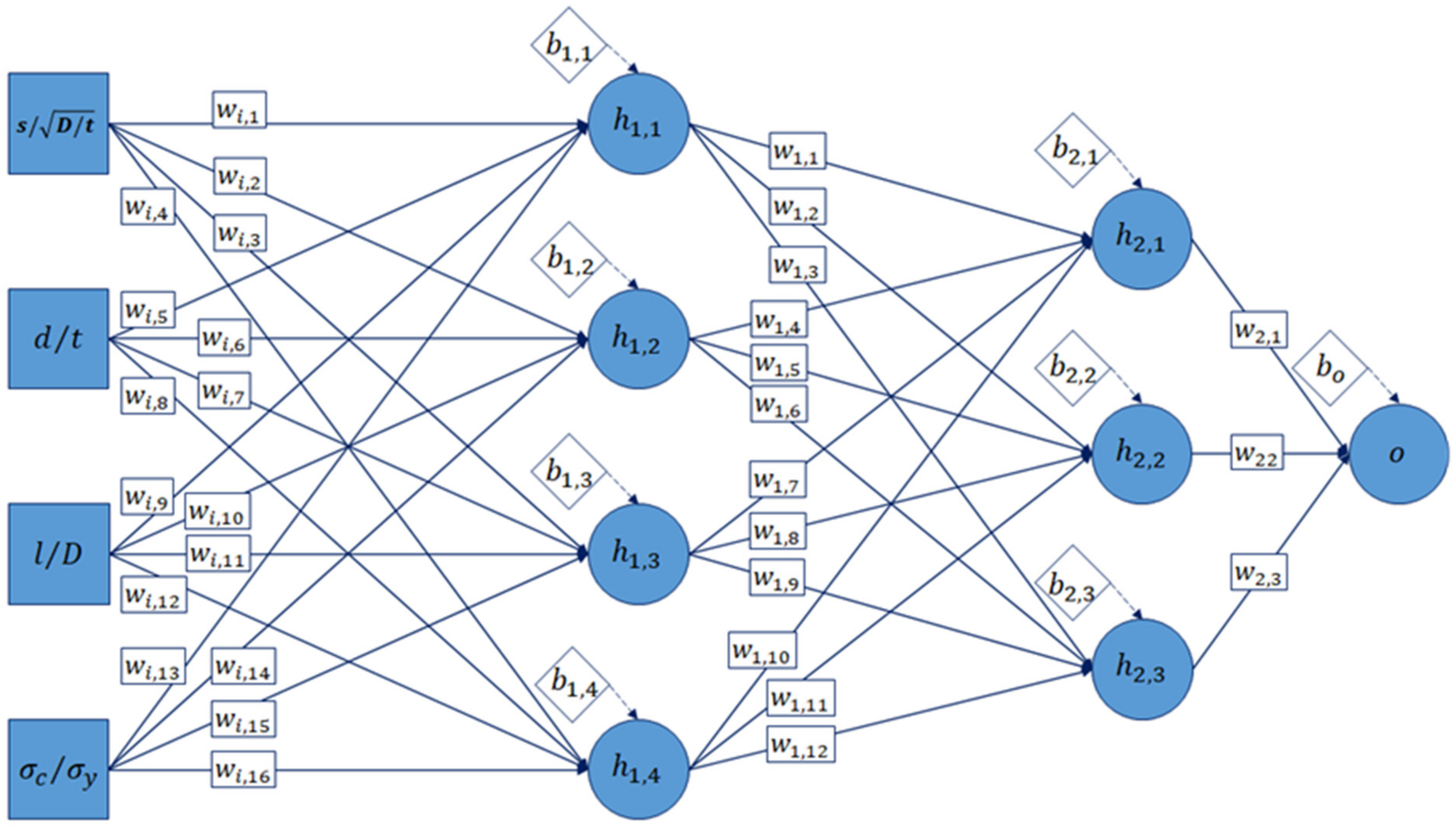
A feed forward neural network to model the relationship between the input and output based on a set of training data was developed using MathWorks MATLAB R2019b. The neural network was trained to receive four inputs, namely normalized defect spacing, defect depth, defect length, and axial compressive stress. The output is the normalized pipe failure pressure. The ANN was developed with two hidden layers. The first and second hidden layer consist of four and three neurons respectively, as illustrated in Figure 7. To optimize the number of hidden layers and neurons in each hidden layer, a convergence test based on the coefficient of determination (R²) value of the ANN model was carried out.

The training data for the ANN model were obtained from the FEA. The failure pressures of corroded pipes obtained using the FEM was normalized by the intact pressure of the pipe before it was used to train the ANN model. The training data consist of 241 sets, as tabulated in

Table 3. ANN training data.

$\mathit{s}/\sqrt{\mathit{D}\mathit{t}}$	${\left(\mathit{d}/\mathit{t}\right)}_{\mathbf{e}}$	${\left(\mathit{l}/\mathit{D}\right)}_{\mathbf{e}}$	${\mathit{\sigma }}_{\mathit{c}}/{\mathit{\sigma }}_{\mathit{y}}$
			0.0	0.2	0.4	0.6	0.8
0.0	0.0	0.0	1.00
0.0	0.2	0.4	0.95	0.94	0.90	0.84	0.72
		0.8	0.91	0.91	0.88	0.80	0.68
		1.2	0.89	0.88	0.86	0.79	0.66
		1.6	0.87	0.87	0.85	0.78	0.66
	0.4	0.4	0.87	0.86	0.83	0.76	0.63
		0.8	0.76	0.76	0.74	0.70	0.58
		1.2	0.72	0.71	0.69	0.66	0.56
		1.6	0.71	0.70	0.66	0.64	0.54
	0.6	0.4	0.75	0.74	0.72	0.68	0.51
		0.8	0.59	0.59	0.57	0.51	0.45
		1.2	0.53	0.51	0.50	0.47	0.42
		1.6	0.48	0.48	0.47	0.45	0.41
	0.8	0.4	0.58	0.56	0.52	0.45	0.41
		0.8	0.38	0.38	0.35	0.32	0.21
		1.2	0.31	0.29	0.26	0.25	0.20
		1.6	0.28	0.27	0.26	0.23	0.20
0.5	0.16	0.49	0.92	0.92	0.89	0.81	0.71
	0.18	0.89	0.89	0.88	0.86	0.80	0.68
	0.19	1.29	0.87	0.86	0.85	0.79	0.66
	0.19	1.69	0.85	0.85	0.84	0.78	0.66
	0.33	0.49	0.83	0.80	0.78	0.73	0.61
	0.36	0.89	0.74	0.72	0.71	0.68	0.58
	0.37	1.29	0.70	0.69	0.68	0.65	0.56
	0.38	1.69	0.68	0.68	0.66	0.64	0.56
	0.49	0.49	0.68	0.66	0.65	0.62	0.53
	0.54	0.89	0.56	0.56	0.54	0.51	0.45
	0.56	1.29	0.51	0.50	0.49	0.46	0.42
	0.57	1.69	0.49	0.49	0.47	0.46	0.41
	0.65	0.49	0.50	0.49	0.48	0.47	0.41
	0.72	0.89	0.36	0.35	0.34	0.29	0.26
	0.74	1.29	0.30	0.30	0.28	0.26	0.24
	0.76	1.69	0.28	0.27	0.26	0.25	0.24
1.0	0.14	0.58	0.93	0.92	0.89	0.84	0.71
	0.16	0.98	0.90	0.90	0.88	0.83	0.70
	0.17	1.38	0.88	0.88	0.86	0.79	0.68
	0.18	1.78	0.88	0.88	0.85	0.79	0.66
	0.27	0.58	0.91	0.84	0.80	0.75	0.64
	0.33	0.98	0.82	0.73	0.72	0.70	0.58
	0.35	1.38	0.77	0.71	0.69	0.66	0.57
	0.36	1.78	0.75	0.69	0.66	0.64	0.56
	0.41	0.58	0.78	0.71	0.70	0.65	0.54
	0.49	0.98	0.63	0.58	0.57	0.54	0.45
	0.52	1.38	0.56	0.51	0.50	0.48	0.44
	0.54	1.78	0.53	0.50	0.49	0.47	0.44
	0.55	0.58	0.58	0.54	0.51	0.51	0.43
	0.65	0.98	0.40	0.36	0.36	0.33	0.28
	0.69	1.38	0.33	0.30	0.28	0.28	0.25
	0.72	1.78	0.30	0.28	0.26	0.25	0.24
2.0	0.10	0.77	0.92	0.92	0.89	0.83	0.71
	0.14	1.17	0.90	0.89	0.88	0.83	0.70
	0.15	1.57	0.87	0.88	0.86	0.79	0.67
	0.16	1.97	0.88	0.88	0.84	0.79	0.66
	0.21	0.77	0.91	0.84	0.80	0.75	0.63
	0.27	1.17	0.82	0.75	0.72	0.70	0.57
	0.31	1.57	0.77	0.71	0.69	0.66	0.57
	0.33	1.97	0.75	0.69	0.66	0.63	0.56
	0.31	0.77	0.78	0.71	0.70	0.65	0.54
	0.41	1.17	0.62	0.58	0.57	0.54	0.45
	0.46	1.57	0.56	0.51	0.50	0.48	0.44
	0.49	1.97	0.53	0.50	0.48	0.47	0.43
	0.42	0.77	0.58	0.54	0.51	0.51	0.43
	0.55	1.17	0.40	0.36	0.36	0.34	0.29
	0.61	1.57	0.32	0.30	0.28	0.28	0.25
	0.65	1.97	0.29	0.28	0.26	0.24	0.24

. The normalized defect spacing, effective depth, effective length, axial compressive stress, and normalized failure pressure are represented by $\mathrm{s}/\sqrt{Dt}$, ${\left(d/t\right)}_e$, ${\left(l/D\right)}_e$, ${\sigma }_c/{\sigma }_y$, and $P_{nf,FEA}$, respectively.

A convergence test was carried out to determine the optimum number of hidden layers and neurons in each hidden layer. The convergence test was based on the regression analysis of the ANN model, where the target was to achieve an R² value of 0.99, with a minimum number of hidden layers and neurons. A total of 12 ANN models were developed and each of their coefficients of determination (R²) was recorded. Initially, the ANN model was trained using one hidden layer with one node. For each subsequent ANN model, the number of neurons in the first hidden layer was increased by 1. When the number of neurons in a hidden layer reached 4, a new hidden layer with one node was added to the subsequent model. As this model is designed to receive four inputs, the maximum number hidden layers and neurons in each hidden layer was set at four, to ensure that the empirical solution that was developed was not overly complex.

Table 4. Performances of the developed ANN models based on their coefficient of determinant.

Model	No. of Hidden Layers	No. of Neurons in Hidden Layer 1	No. of Neurons in Hidden Layer 2	No. of Neurons in Hidden Layer 3	R2 Value
1	1	1	-	-	0.93
2	1	2	-	-	0.93
3	1	3	-	-	0.94
4	1	4	-	-	0.94
5	2	4	1	-	0.95
6	2	4	2	-	0.98
7	2	4	3	-	0.99
8	2	4	4	-	0.99
9	3	4	4	1	0.97
10	3	4	4	2	0.96
11	3	4	4	3	0.93
12	3	4	4	4	0.91

summarizes the R² value obtained for each model developed.

Based on all the R² values obtained, it was found that Models 7 and 8 resulted in the most accurate failure pressure prediction. Both the models produced a R² value of 0.99. Model 7 consisted of four neurons in the first hidden layer and three neurons in the second hidden layer, having one less neuron than Model 8. As such, Model 7 was utilized for the development of an empirical solution to ensure the simplicity of the equations without compromising the accuracy of the outcome.

The regression plots of Model 7 extracted from MathWorks MATLAB R2019b that represent the training, validation, testing, and the combination of all the three plots are illustrated in Figure 8. The linear regression line of best fit of the output of the ANN is represented by the solid lines in the plot, with dashed lines representing the training data. Based on Figure 8, it was observed that the solid lines and dashed line in each plot almost overlap completely, indicating that Model 7 is highly capable of producing results that are similar to that of the training data.

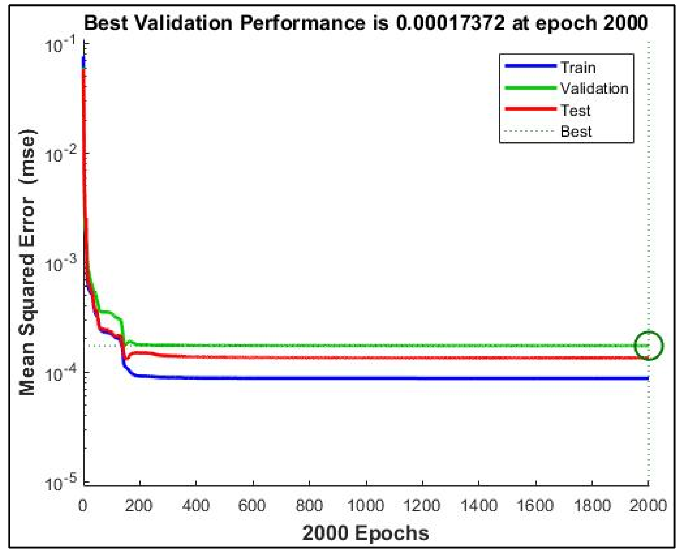
The number of epochs or iterations which determines the number of times the learning algorithm will learn from the entire training dataset was set to a maximum of 2000 with 1500 validation checks. Fifteen percent of the training dataset is reserved as the validation dataset and is not introduced to the neural network during training. After each iteration, the algorithm calculates the mean square error of the validation dataset, as illustrated in Figure 9. The iteration is stopped upon reaching the maximum number of epoch or validation checks. The weights and biases at the epoch that produces the best validation performance is chosen and applied to the ANN.

The ability of the ANN to produce outcomes close to the training data is measured using the coefficient of determination (R²) of the model. The R² value ranges from 0.0 to 1.0, with a greater R² value indicating a better goodness of fit, which is the distance between the fitted line of the ANN’s regression plot and the training data points.

2.4. Material Properties

A rate-independent plasticity model utilizing von Mises yield criterion and isotropic hardening rule was employed in the non-linear structural analysis. A high toughness pipe grade of API 5L X80 was utilized in this study and the mechanical properties of the pipe body as well as the end cap are summarized in

Table 5. Mechanical properties of the API 5L X80 [21].

Properties	Pipe Body	Pipe End Cap
Modulus of elasticity, E	210 GPa	210 TPa
Poisson’s ratio, υ	0.3	0.3
Yield strength, σy	531.0 MPa	-
Ultimate tensile strength, σu	655.0 MPa	-
True ultimate tensile strength, σ×u	718.2 MPa	-

. In this analysis, the endplate was assumed to be a rigid body that does not undergo deformation. The material properties of the pipe body are represented by a nonlinear true stress-strain curve of the material, as illustrated in Figure 10. To accommodate high material nonlinearity in the pipe body, material stress stiffening, large strain, and displacements were considered.

3. Validation of the Finite Element Method

Before carrying out FEA, the FEM was validated against an actual full scale burst test to ensure its accuracy and reliability. The validation was carried out based on burst tests conducted by Bjorney et al. and Benjamin et al. [55,56].

Table 6. FEM failure pressure validation against full scale burst tests by Bjorney et al. for single corrosion defect [55].

Grade	Specimen	d (mm)	l (mm)	w (mm)	σl (MPa)	Burst Pressure (MPa)	FEA Failure Pressure (MPa)	Percentage Difference (%)
X52	Test 1	5.15	243	154.5	0.0	23.2	22.95	−1.08
	Test 5	3.09	162	30.9	48.0	28.6	28.35	−0.87
	Test 6	3.09	162	30.9	84.0	28.7	27.00	−5.92

summarizes burst test results by Bjorney et al. for burst pressures of single corrosion defect subjected to internal pressure only, and combined loading (internal pressure and axial compressive stress) [57].

Table 7. FEM failure pressure validation against full scale burst tests by Benjamin et al. for interacting corrosion defects [56].

Grade	Specimen	$\mathit{d}$	$\mathit{l}$	$\mathit{w} \left(\mathbf{mm}\right)$	${\mathit{s}}_{\mathit{l}}\left(\mathbf{mm}\right)$	${\mathit{s}}_{\mathit{c}}\left(\mathbf{mm}\right)$	Burst Pressure (MPa)	FEA Failure Pressure (MPa)	Percentage Difference (%)
X80	IDTS 2	5.39	39.6	31.9	0.0	0.0	22.68	22.40	−1.23
	IDTS 3	5.32	39.6	31.9	20.5	0.0	20.31	20.12	−0.94
	IDTS 4	5.62	39.6	32.0	0.0	9.9	21.14	20.62	−2.46

summarizes burst test results by Benjamin et al. for burst pressures of interacting defects subjected to internal pressure only [56].

For single defects, the largest percentage difference between the failure pressure obtained using FEM and actual full scale burst tests was 5.92%. As for interacting defects, the largest percentage difference was 2.46%. A positive percentage difference indicates overestimation, while a negative value indicates conservatism. Based on the validation, it was observed that this method results in a slight conservatism that is within the range of 6%. Hence, it is evident that the FEM is reliable to be used as a failure pressure data generation tool for the training of the ANN.

To ensure a good correlation between the intact pressure obtained using FEM and theoretical calculations, the intact pressure, $P_i$, value was compared with the maximum hoop stress theory represented by Equation (2) [2]. Based on this theory, the intact pressure of the pristine pipe is 51.3 MPa and the intact pressure of the same pipe obtained using FEM was 50.94 MPa, with a percentage difference of −0.70%. There is therefore a strong correlation between these two methods.

$$P_i=\frac{{\mathsf{\sigma }}_{UTS} t}{r_i}$$

(2)

where $r_i$ is the pipe internal radius.

4. Results and Discussion

4.1. Comparison of Pipe Failure Pressure Prediction Using FEA and DNV Method

The DNV method was primarily developed to assess the integrity of medium toughness pipelines, as the validation of this method was based on full-scale burst tests conducted on pipes of grades API 5L X45 to API 5L X65. This method incorporates internal pressure and axial compressive stress for the failure pressure prediction of pipelines with single corrosion defects. However, only 7.25% of the validation tests considered axial compressive stress. As such, it can be concluded that the validation of the method for corroded pipes subjected to both internal pressure and axial compressive stress is not as comprehensive as the validation of the method for the assessment of corroded pipes subjected to internal pressure only [15].

As for interacting defects, this method considers internal pressure only. Based on Figure 11, the DNV method results in conservative failure pressure predictions compared to the FEM for API 5L X80 pipes with interacting corrosion defects subjected to internal pressure only. It was observed that for defect depths of 0.20 to 0.60, the conservativeness of the DNV method is more significant, with a percentage difference ranging from −14.29% to −9.59%. As the defect depth is increased to 0.80, the conservativeness of the DNV method reduces, with a percentage difference ranging from −11.34% to −5.11%.

Theoretically, the failure pressure of a corroded pipe with two longitudinally aligned corrosion defects in close proximity is lower than that of a pipe with single corrosion defect of the same dimensions [57]. This is caused by the stress and strain disturbances that occur in each corrosion defect. As each defect causes a disruption in the distribution of stress and strain across the pipe, an overlap region of stress and strain concentration is created [58,59]. This results in a significant decrease in failure pressure of the corroded pipe. Based on Figure 12, for FEA, it is observed that there is an increase in the failure pressure of the corroded pipe when the normalized defect spacing is increased from 0.0 to 1.2 for normalized defect depths of 0.20 to 0.80. The failure pressure begins to increase as the overlap region reduces in size, due to an increase in the defect spacing. When the overlap region becomes smaller, the interaction between the defects reduces and the defects can be treated as single defects.

However, when the DNV method was used, it was observed that failure pressures were conservative by a range of 14.4 to 18.9% for normalized defect depths of 0.2 to 0.8. Above a normalized defect spacing of 0.8, the failure pressure begins to plateau. However, based on FEA, the failure pressure begins to plateau only at a defect spacing of 1.2. This shows the conservativeness of the DNV method when used to assess the failure pressure of high toughness steels. Overly conservative predictions result in unwarranted and premature pipe repairs that are costly [19].

4.2. Development of an Empirical Equation for the Failure Pressure Prediction of a Corroded Pipeline

The development of the empirical equation to predict the failure pressure of a pipe with corrosion defects was based on the weights and biases of the ANN model represented by Equations (3)–(5).

$$\left[\begin{array}{c}{\mathrm{h}}_{1,1}\\ {\mathrm{h}}_{1,2}\\ {\mathrm{h}}_{1,3}\\ {\mathrm{h}}_{1,4}\end{array}\right]=\left[\begin{array}{cccc}{\mathrm{w}}_{i,1}& {\mathrm{w}}_{i,5}& {\mathrm{w}}_{i,9}& {\mathrm{w}}_{i,13}\\ {\mathrm{w}}_{i,2}& {\mathrm{w}}_{i,6}& {\mathrm{w}}_{i,10}& {\mathrm{w}}_{i,14}\\ {\mathrm{w}}_{i,3}& {\mathrm{w}}_{i,7}& {\mathrm{w}}_{i,11}& {\mathrm{w}}_{i,15}\\ {\mathrm{w}}_{i,4}& {\mathrm{w}}_{i,8}& {\mathrm{w}}_{i,12}& {\mathrm{w}}_{i,16}\end{array}\right]\left[\begin{array}{c}{\left(s/\sqrt{D/t}\right)}_n\\ {\left(d/t\right)}_n\\ {\left(l/d\right)}_n\\ {\left(\sigma c/\sigma y\right)}_n\end{array}\right]+\left[\begin{array}{c}{\mathrm{b}}_{1,1}\\ {\mathrm{b}}_{1,2}\\ {\mathrm{b}}_{1,3}\\ {\mathrm{b}}_{1,4}\end{array}\right]$$

(3)

$$\left[\begin{array}{c}{\mathrm{h}}_{2,1}\\ {\mathrm{h}}_{2,2}\\ {\mathrm{h}}_{2,3}\end{array}\right]=\left[\begin{array}{cccc}{\mathrm{w}}_{1,1}& {\mathrm{w}}_{1,4}& {\mathrm{w}}_{1,7}& {\mathrm{w}}_{1,10}\\ {\mathrm{w}}_{1,2}& {\mathrm{w}}_{1,5}& {\mathrm{w}}_{1,8}& {\mathrm{w}}_{1,11}\\ {\mathrm{w}}_{1,3}& {\mathrm{w}}_{1,6}& {\mathrm{w}}_{1,9}& {\mathrm{w}}_{1,12}\end{array}\right]\left[\begin{array}{c}a\left({\mathrm{h}}_{1,1}\right)\\ a\left({\mathrm{h}}_{1,2}\right)\\ a\left({\mathrm{h}}_{1,3}\right)\\ a\left({\mathrm{h}}_{1,4}\right)\end{array}\right]+\left[\begin{array}{c}{\mathrm{b}}_{2,1}\\ {\mathrm{b}}_{2,2}\\ {\mathrm{b}}_{2,3}\end{array}\right]$$

(4)

$$o_n=\left[\begin{array}{ccc}{\mathrm{w}}_{2,1}& {\mathrm{w}}_{2,2}& {\mathrm{w}}_{2,3}\end{array}\right]\left[\begin{array}{c}a\left({\mathrm{h}}_{2,1}\right)\\ a{(\mathrm{h}}_{2,2})\\ a{(\mathrm{h}}_{2,3})\end{array}\right]+\left[{\mathrm{b}}_o\right]$$

(5)

The ANN model normalizes the input values so that the values fall within the range of −1 to 1 before the values at the input neurons are multiplied by the respective weights and transferred to the neuron in the next layer. The normalized input values, $i_n$, can be calculated using Equation (6). Likewise, the output value, $o$, is also a normalized value. Hence, it needs to be denormalized using Equation (7).

$$i_n=\frac{\left(i_{n, max}-i_{n, min}\right)\left(i-i_{min}\right)}{\left(i_{max}-i_{min}\right)}+i_{n, min}$$

(6)

where

• $i_{n, max}$ is the maximum normalized input value,
• $i_{n, min}$ is the minimum normalized input value,
• $i$ is the input value,
• $i_{min}$ is the minimum input value of the training data, and
• $i_{max}$ is the maximum input value of the training data.

$$o=\frac{\left(o_n-o_{n, min}\right)\left(o_{max}-o_{min}\right)}{\left(o_{n, max}-o_{n, min}\right)}+o_{min}$$

(7)

where

• $o_n$ is the normalized output value,
• $o_{n,min}$ is the normalized minimum output value of the training data,
• $o_{n,max}$ is the normalized maximum output value of the training data,
• $o_{max}$ is the maximum output value of the training data, and
• $o_{min}$ is the minimum output value of the training data.

The steps involved in predicting the failure pressure of a pipeline with corrosion defect(s) are summarized below:

• Step 1: Calculation of the normalized effective length and depth of defect.

  $${\left(l/D\right)}_e=\frac{l_1+\left(s_1+l_2\right)}{t}$$

  (8)

  $${\left(d/t\right)}_e=\frac{\left(\frac{d_1{l}_1+d_2{l}_2}{l_{1,2}}\right)}{D}$$

  (9)
• Step 2: Normalization of input parameters.

  $${\left(s/\sqrt{D/t}\right)}_n=\frac{2{\left(s/\sqrt{D/t}\right)}_i}{3}-1$$

  (10)

  $${\left(l/D\right)}_e{}_n=\frac{2{\left(l/D\right)}_e}{2.15}-1$$

  (11)

  $${\left(d/t\right)}_e{}_n=2.5{\left(d/t\right)}_e-1$$

  (12)

  $${\left(\sigma c/\sigma y\right)}_n=2.5{\left(\sigma c/\sigma y\right)}_i-1$$

  (13)
• Step 3: Calculation of the normalized output value.

  $$\left[\begin{array}{c}{\text{h}}_{1,1}\\ {\text{h}}_{1,2}\\ {\text{h}}_{1,3}\\ {\text{h}}_{1,4}\end{array}\right]=\left[\begin{array}{c}-0.0830{\left(s/\sqrt{D/t}\right)}_n+0.2350{\left(l/D\right)}_e{}_n+1.4834{\left(d/t\right)}_e{}_n-1.9408{\left(\sigma c/\sigma y\right)}_n+2.2349\\ 0.2086{\left(s/\sqrt{D/t}\right)}_n-0.1390{\left(l/D\right)}_e{}_n+0.1719{\left(d/t\right)}_e{}_n+0.0065{\left(\sigma c/\sigma y\right)}_n-0.2576\\ -0.07195{\left(s/\sqrt{D/t}\right)}_n-2.645{\left(l/D\right)}_e{}_n-0.50324{\left(d/t\right)}_e{}_n-0.1314{\left(\sigma c/\sigma y\right)}_n-1.6399\\ -0.2208{\left(s/\sqrt{D/t}\right)}_n+0.1131{\left(l/D\right)}_e{}_n-0.7073{\left(d/t\right)}_e{}_n-0.0425{\left(\sigma c/\sigma y\right)}_n-0.6017\end{array}\right]$$

  (14)

  $$\left[\begin{array}{c}{\mathrm{h}}_{2,1}\\ {\mathrm{h}}_{2,2}\\ {\mathrm{h}}_{2,3}\end{array}\right]=\left[\begin{array}{c}0.0208a\left({\mathrm{h}}_{1,1}\right)+1.0157a\left({\mathrm{h}}_{1,2}\right)-0.2254a\left({\mathrm{h}}_{1,3}\right)-2.2751a\left({\mathrm{h}}_{1,4}\right)-2.5736\\ 0.3627a\left({\mathrm{h}}_{1,1}\right)+3.0005a\left({\mathrm{h}}_{1,2}\right)+0.0389a\left({\mathrm{h}}_{1,3}\right)+1.9307a\left({\mathrm{h}}_{1,4}\right)+1.7659\\ 2.3000a\left({\mathrm{h}}_{1,1}\right)+0.6237a\left({\mathrm{h}}_{1,2}\right)+1.2367a\left({\mathrm{h}}_{1,3}\right)-1.7914a\left({\mathrm{h}}_{1,4}\right)-4.5105\end{array}\right].$$

  (15)

  $$o_n=-2.5645a{(\mathrm{h}}_{2,1})+0.9479a{(\mathrm{h}}_{2,2})+1.1226a{(\mathrm{h}}_{2,3})-1.2962$$

  (16)

The values of $a\left({\mathrm{h}}_{1,1}\right)$ to $a\left({\mathrm{h}}_{2,3}\right)$ are calculated using Equation (17).

$$a\left({\mathrm{h}}_{x,y}\right)=\frac{2}{1+e^{-2\left({\mathrm{h}}_{x,y}\right)}}-1$$

(17)

• Step 4: Denormalization of output value, $P_{nf,Eq}$

  $$P_{nf,Eq}=0.385o_n+0.615$$

  (18)
• Step 5: Calculation of failure pressure, $P_{f,Eq}$.

  $$P_i=\frac{\sigma {\times }_{UTS}t}{r_i}$$

  (19)

  $$P_{f,Eq}=P_{nf,Eq}\times P_i$$

  (20)

4.3. Evaluation of the New Corroded Pipeline Failure Pressure Assessment Method

Since the equations in the newly developed corrosion assessment method were extracted from the ANN, the R² value of the new method is similar to that of the ANN, which is 0.999. This indicates that the method results in failure pressure predictions that are very close to the results obtained using FEA, which was used as the training data for the ANN model. Based on the maximum hoop stress theory, the calculation of the intact pressure of the pristine pipe model resulted in a value of 51.30 MPa, while the intact pressure obtained using FEM was 50.94 MPa. The intact pressure of the pristine pipe obtained from the newly developed failure pressure assessment method was calculated to be 51.36 MPa. The comparison of the intact pressure values obtained using the three methods are summarized in

Table 8. Comparison of the intact pressure values of the pristine pipe.

Maximum Hoop Stress Theory (A) (MPa)	FEM (B) (MPa)	Newly Developed Method (C) (MPa)	Percentage Difference between (A) and (C) (%)	Percentage Difference between (B) and (C) (%)
51.30	50.94	51.36	0.12	0.84

. There is good correlation between the three methods, with the percentage difference between the failure pressure obtained using the maximum hoop stress and the empirical equation is 0.12%, while the percentage difference between the failure pressure obtained using FEM and the empirical equation is 0.84%.

Figure 13 depicts the percentage difference between the failure pressure predicted using FEM and the empirical equation for the parameters used to train the ANN. The percentage differences fall within −9.90% to 0.67%, with a standard deviation of 2.22. Since the percentage differences fall within 4.5 standard deviations of the mean, the probability of obtaining a failure pressure with a percentage error greater than 9.99% is 1 in 147,160. Only 1.24% of the 241 datasets resulted in overestimation with a maximum percentage difference of only 0.67%. Hence, it can be said that this method is reliable.

Due to the lack of data on full scale burst tests of high toughness pipes subjected to internal pressure and axial compressive stress for interacting defects, FEM was used to further validate the new failure pressure prediction method based on a set of arbitrary data for API 5L X80 material with a σ×_UTS value of 718.2 MPa.

Table 9. Comparison of the failure pressure obtained using FEA and the empirical equation.

$\mathit{s}/\sqrt{\mathit{D}/\mathit{t}}$	$\mathit{d}/\mathit{t}$	$\mathit{l}/\mathit{D}$	$\mathit{\sigma }\mathit{c}/\mathit{\sigma }\mathit{y}$	${\mathit{P}}_{\mathit{n}\mathit{f},\mathit{F}\mathit{E}\mathit{A}}$	${\mathit{P}}_{\mathit{n}\mathit{f},\mathit{E}\mathit{q}}$	Percentage Difference (%)
0.25	0.65	0.09	0.30	0.93	0.91	−2.28
0.25	0.65	0.09	0.60	0.84	0.84	0.02
0.25	1.45	0.10	0.30	0.91	0.89	−1.72
0.25	1.85	0.10	0.30	0.90	0.89	−1.05
0.25	1.85	0.10	0.60	0.83	0.81	−2.17
0.25	0.65	0.28	0.30	0.82	0.78	−4.51
0.25	0.65	0.28	0.60	0.72	0.73	0.35
0.25	1.45	0.34	0.60	0.68	0.66	−2.32
0.25	1.45	0.44	0.60	0.59	0.57	−3.21
0.25	1.45	0.48	0.30	0.58	0.55	−4.39
0.25	0.65	0.51	0.60	0.54	0.53	−1.32
0.25	1.45	0.53	0.60	0.51	0.48	−5.86
0.25	0.45	0.72	0.50	0.40	0.37	−7.54
0.25	0.65	0.74	0.60	0.31	0.28	−8.99
0.25	1.45	0.77	0.50	0.26	0.24	−8.02
0.25	1.45	0.77	0.60	0.26	0.23	−8.63
0.30	1.05	0.47	0.30	0.62	0.57	−7.34
0.30	0.65	0.27	0.30	0.83	0.79	−4.63
0.40	1.47	0.43	0.60	0.58	0.58	−0.39
0.40	1.87	0.53	0.50	0.52	0.49	−5.63
0.70	0.73	0.37	0.30	0.73	0.70	−4.28
0.70	1.53	0.50	0.60	0.53	0.50	−5.25
0.70	1.93	0.75	0.50	0.26	0.24	−5.90
0.90	0.76	0.43	0.50	0.63	0.61	−3.62
0.90	1.56	0.20	0.30	0.85	0.82	−3.58
1.00	0.58	0.40	0.20	0.71	0.71	−0.09
0.50	0.89	0.60	0.40	0.45	0.43	−4.09
0.80	1.75	0.30	0.70	0.66	0.64	−2.35
0.20	0.45	0.20	0.30	0.89	0.86	−3.46
0.30	0.65	0.40	0.60	0.68	0.63	−6.95
0.40	1.45	0.60	0.30	0.45	0.43	−5.47
0.80	1.05	0.30	0.60	0.72	0.69	−3.52
0.90	0.65	0.20	0.30	0.89	0.85	−4.72
1.00	1.47	0.40	0.60	0.60	0.59	−0.90
1.20	1.87	0.60	0.40	0.41	0.39	−4.94

summarizes the parametric details, the failure pressure predictions using FEM and the empirical equation, and the percentage difference between the methods. A negative percentage difference indicates a conservative prediction, while a positive value indicates overestimation.

Based on Table 9, the Root Mean Square Error (RMSE) of the regression analysis conducted on the obtained results is 0.01, indicating that the predicted failure pressure value is very close to the failure pressure obtained using FEA. The percentage difference between these two methods falls between −8.99% and 0.35%. The predicted failure pressures fall within the 4.5 sigma range of 9.99%. This is true for normalized defect spacings of 0.00 to 2.00, normalized effective defect lengths of 0.00 to 1.97, normalized effective defect depths of 0.00 to 0.80, and normalized axial compressive stress of 0.00 to 0.80.

4.4. Extensive Parametric Studies Using the Empirical Equation

The empirical equation was used to conduct an extensive parametric study to determine the effects of defect spacing, defect depth, defect length, and axial compressive stress on an API 5L X80 corroded pipe with interacting corrosion defects. The parameters used in this study and the results are represented in the graphs below. In this parametric study, the failure pressure of pipes subjected to internal pressure only was used as reference data to study the effects of normalized defect spacing, normalized defect length, normalized defect depth, and normalized axial compressive stress on the normalized failure pressure of a pipe when axial compressive stress was introduced.

4.4.1. Effects of Defect Spacing on the Failure Pressure of a Pipe with Interacting Defects

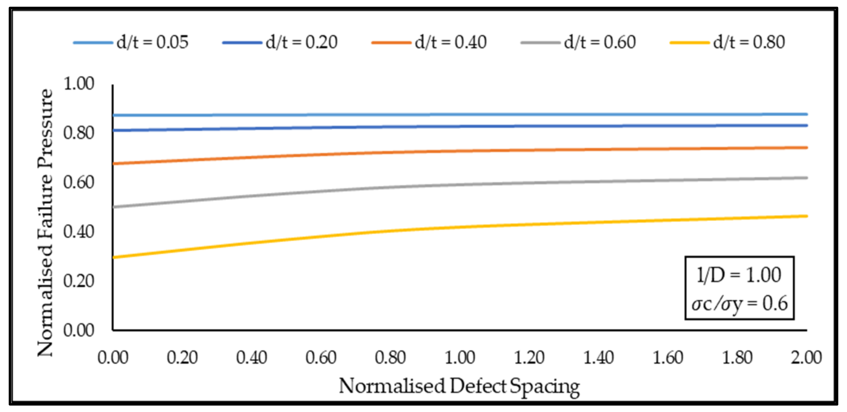
Based on Figure 14, at a constant normalized defect length of 1.00 and axial compressive stress of 0.60, the normalized failure increases as the normalized defect spacing was increased from 0.00 to 1.60. However, this increase is more significant for normalized defect depths of 0.60 to 0.80. The maximum normalized pressure drop observed was 55.12% for a normalized defect depth of 0.80. These results were expected as in the presence of interacting defects, there is a region of stress overlap which causes the failure pressure to be lower than that of a single defect. The normalized defect spacing has an increasingly significant effect on the normalized failure pressure of a pipe with interacting corrosion defects as the depth of the corrosion increases. This pattern was also observed for normalized defect depths of 0.05, 0.20, 0.40, and 0.80.

4.4.2. Effects of Defect Depth on the Failure Pressure of a Pipe with Interacting Defects

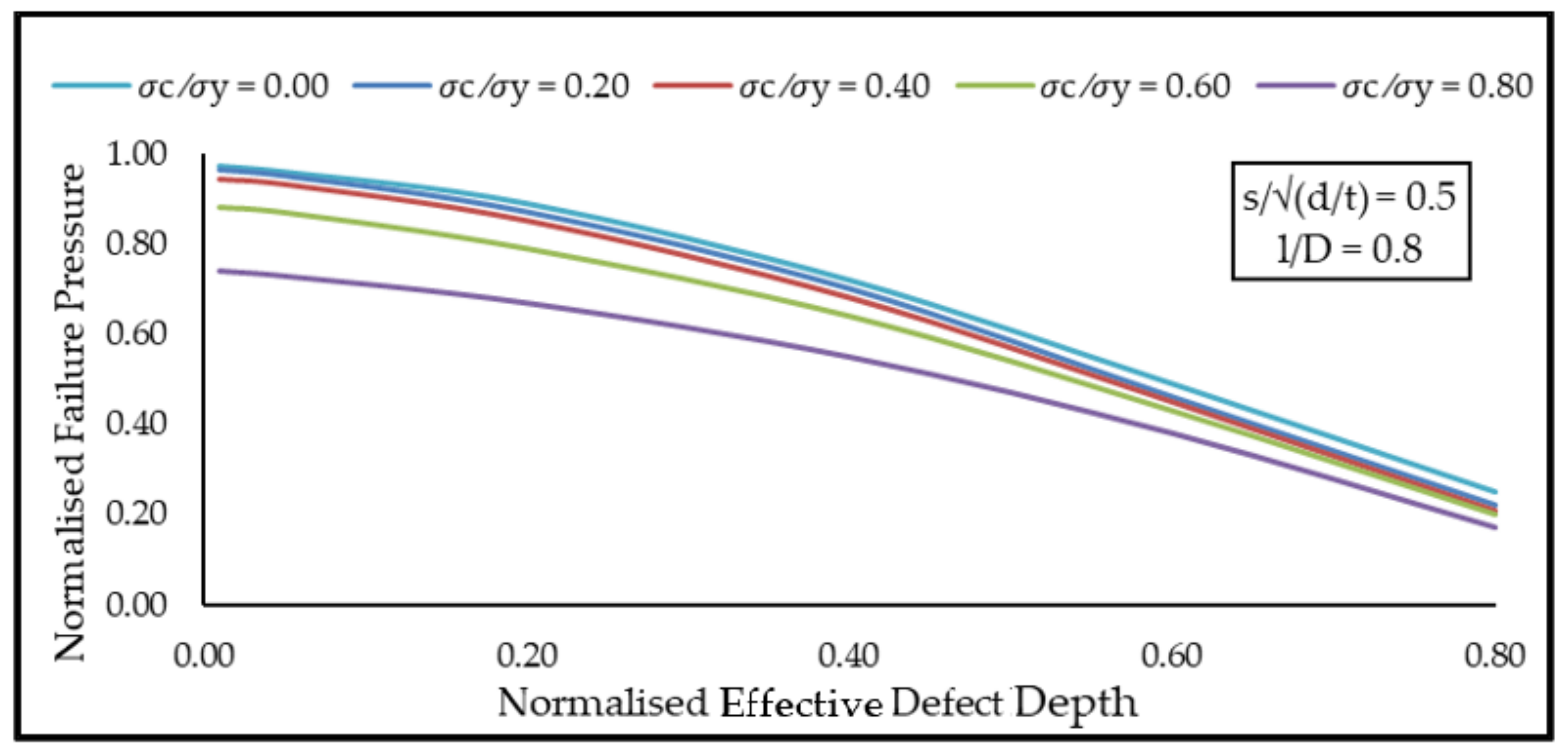
Based on Figure 15, at a constant normalized effective defect length of 0.80 and normalized defect spacing of 0.5, the normalized failure pressure decreases drastically as the normalized effective defect depth was increased for normalized axial compressive stress values of 0.00 to 0.80. The maximum normalized pressure drop observed based on normalized axial compressive stress was 76.29% at a normalized axial compressive stress value of 0.40. This indicates that the normalized effective defect depth has a high influence on the normalized failure pressure of a pipe. As the normalized effective defect depth approaches a value of 0.80, the normalized failure pressure begins to converge to a point. This pattern was also observed for effective defect lengths of 0.05, 0.20, 0.40, 0.60, 1.00, and 1.20, as well as for normalized defect spacings of 1.00 and 2.0.

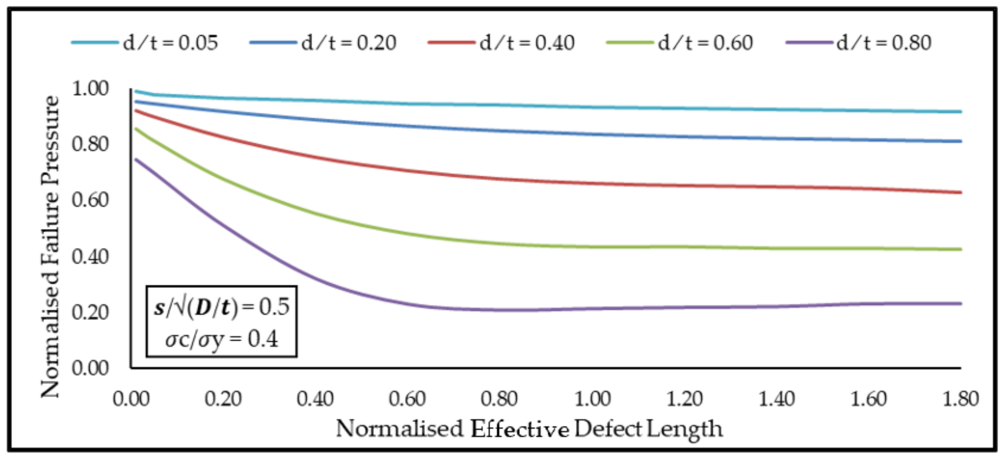
Based on Figure 16, at a constant normalized defect spacing of 0.5 and normalized axial compressive stress of 0.40, the influence of normalized effective defect depth on the decrease in normalized failure pressure can be observed in more detail as the normalized effective defect lengths are increased from 0.05 to 1.80. Generally, it was observed that the normalized failure pressure decreases gradually as the normalized effective defect depth was increased. The maximum normalized failure pressure reduction observed based on normalized effective defect lengths of 0.00 to 1.80 was 74.73% for a normalized effective defect length of 1.60. As the normalized effective defect depth is increased from 0.0 to 0.8, the decrease in failure pressure is more drastic for increasing values of normalized effective defect length. This indicates that the normalized effective defect depth greatly influences the normalized failure pressure of a pipe under axial loading and internal stress. This pattern was also observed for normalized axial compressive stress values of 0.2, 0.6, and 0.8, as well as for normalized defect spacings of 1.00 and 2.00.

4.4.3. Effects of Defect Length on the Failure Pressure of a Pipe with Interacting Defects

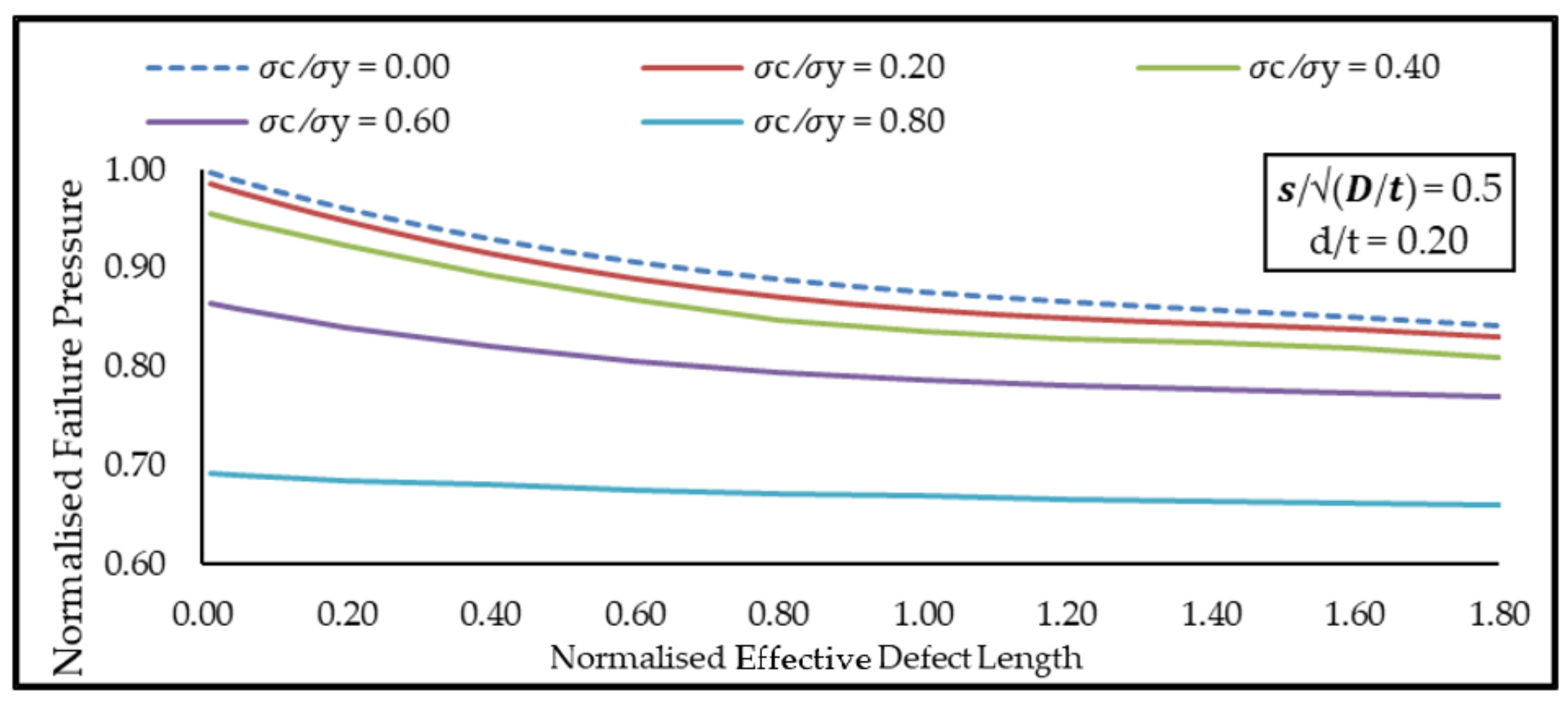
Based on Figure 17, for normalized effective defect lengths of 0.05 to 1.80, the decrease in normalized failure pressure was observed to be more significant for normalized axial compressive stress values of 0.00 to 0.60 for normalized effective defect lengths of 0.05 to 0.40. For increasing values of normalized effective defect lengths, it was observed that the failure pressure decreased by a maximum of 15.31% for a normalized axial compressive stress of 0.20. This pattern is similar for a normalized effective defect depth of 0.05 and 0.40 with a maximum normalized failure pressure decrease of 8.16% and 30.85%, respectively.

This decrease is more significant as the normalized effective defect length is increased for normalized effective defect depth values of 0.60 and 0.80. Under these conditions, the maximum decrease in failure pressure was 48.86% and 67.57%, respectively, for normalized axial compressive stress values of 0.00 to 0.80. A drastic decrease in the normalized failure pressure for normalized effective defect lengths of 0.00 to 0.80 was observed indicating that the normalized effective defect length significantly influences the failure pressure of a pipe when the normalized effective defect depth ranges from 0.60 to 0.80. For the case of normalized defect depth of 0.80, the decrease in failure pressure is illustrated in Figure 18. Furthermore, it was also observed that the normalized failure pressure plateaus, as the normalized effective defect length increases from 0.80 to 1.80, as depicted in Figure 17 and Figure 18. This pattern was also observed for normalized defect spacings of 1.00 and 2.00.

Based on Figure 19, at a constant normalized axial compressive stress of 0.40, the influence of normalized effective defect length on the decrease in normalized failure pressure is more significant as the normalized effective defect depths are increased from 0.00 to 0.80. Since the maximum decrease in normalized failure pressure was only 10.00% for normalized effective defect depths of 0.05 to 0.20 when the normalized effective defect length was increased from 0.00 to 1.80, it indicates that the influence of normalized effective defect length is insignificant under these conditions. As the normalized effective defect length was increased from 0.80 to 1.80 for each of the normalized effective defect depth values, it was observed that its influence on normalized failure pressure was also insignificant. The maximum drop in normalized failure pressure in this region was only 9.65%. This indicates that for normalized effective defect depths of 0.00 to 0.80, normalized effective defect lengths of 0.00 to 0.80 significantly influence the normalized failure pressure. This pattern was observed to be similar for all other values of normalized defect spacings and normalized axial compressive stresses investigated in this parametric study.

4.4.4. Effects of Axial Compressive Stress on the Failure Pressure of a Pipe with Interacting Defects

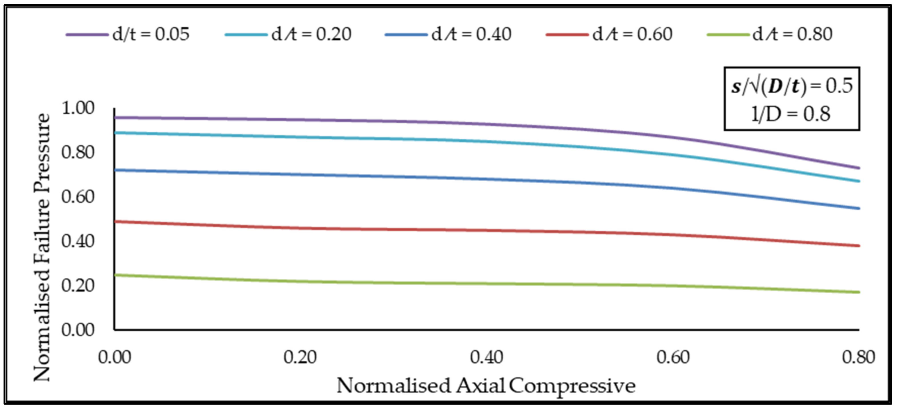
Based on Figure 20, at a constant normalized defect spacing of 0.5 and normalized effective defect length of 0.80, the normalized failure pressure decreases insignificantly for normalized axial compressive stress values of 0.0 to 0.4 for normalized effective defect depth values of 0.05 to 0.60. Under these conditions, the maximum normalized failure pressure decrease was observed to be only 5.41% at a normalized effective defect depth of 0.40. For a normalized effective defect depth of 0.80, this reduction in failure pressure was observed to be comparatively higher with a 17.86% decrease in failure pressure for normalized axial compressive stress values of 0.00 to 0.40. For normalized axial compressive stress values of 0.40 to 0.60, the normalized failure pressure drops significantly by a maximum of 22.09% for a normalized effective defect depth of 0.40 at a normalized axial compressive stress of 0.80. This indicates that when a normalized axial compressive stress value of 0.4 to 0.8 is imposed on a pipe, it causes a significant decrease in the normalized failure pressure of the pipe. This pattern was also observed for all other normalized effective defect length values as well as normalized defect spacings of 1.00 and 2.00.

4.5. Recommendations for Future Studies

The empirical equation is applicable for the prescribed range and material only. Future studies using a greater number of ANN training datasets that consist of different types of material and varying parameters of corrosion defects should be done to increase the robustness and application of the equation.

5. Conclusions

An empirical equation for failure pressure prediction of corroded high toughness pipelines with interacting defects subjected to internal pressure and axial compressive stress was developed. The obtained results proved that ANNs are capable of accurately predicting the failure pressure of a corroded pipeline, provided that it has been trained sufficiently, and is suitable to be used as a tool to develop empirical equations based on its weights and biases. By doing so, a level 3 corrosion assessment method can be reduced to a level 1 assessment level complexity which allows the user to carry out failure pressure calculations easily using a single spreadsheet.

The equation predicted failure pressures for API 5L X80 pipes with a R² value of 0.99 for normalized defect spacings of 0.00 to 2.00, normalized effective defect lengths of 0.00 to 1.97, normalized effective defect depths of 0.00 to 0.80, and normalized axial compressive stress of 0.00 to 0.80, for API 5L X80 pipe grade. This equation is therefore suitable for the failure pressure prediction of high toughness pipes ranging from API 5L X80 material with normalized defect length, normalized defect depth, and normalized axial compressive stress that are within the mentioned ranges.

References

1. Ren, L.; Jiang, T.; Jia, Z.-G.; Li, D.-S.; Yuan, C.-L.; Li, H.-N. Pipeline corrosion and leakage monitoring based on the distributed optical fiber sensing technology. Measurement 2018, 122, 57–65. [Google Scholar] [CrossRef]
2. Arumugam, T.; Karuppanan, S.; Ovinis, M. Finite element analyses of corroded pipeline with single defect subjected to internal pressure and axial compressive stress. Mar. Struct. 2020, 72, 102746. [Google Scholar] [CrossRef]
3. Belachew, C.T.; Ismail, M.C.; Karuppanan, S. Burst Strength Analysis of Corroded Pipelines by Finite Element Method. J. Appl. Sci. 2011, 11, 1845–1850. [Google Scholar] [CrossRef]
4. Cosham, A.; Palmer, A.; Hopkins, P. The Assessment of Corrosion in Pipeline-Guidance in the Pipeline Defect Assessment Manual (PDAM). In Proceedings of the 2004 in Pipeline Pigging and Integrity Management Conference, Amsterdam, The Netherlands, 17–18 May 2004; pp. 1–18. [Google Scholar]
5. Ahammed, M.; Melchers, R. Probabilistic analysis of underground pipelines subject to combined stresses and corrosion. Eng. Struct. 1997, 19, 988–994. [Google Scholar] [CrossRef]
6. Chauhan, V.; Swankie, T.D.; Espiner, R.; Wood, I. Developments in Methods for Assessing the Remaining Strength of Corroded Pipelines. In NACE Corrosion 2009 Conference Expo; NACE International: Houston, TX, USA, 2009; pp. 1–29. [Google Scholar]
7. Mokhtari, M.; Melchers, R. A new approach to assess the remaining strength of corroded steel pipes. Eng. Fail. Anal. 2018, 93, 144–156. [Google Scholar] [CrossRef]
8. Fekete, G.; Varga, L. The effect of the width to length ratios of corrosion defects on the burst pressures of transmission pipelines. Eng. Fail. Anal. 2012, 21, 21–30. [Google Scholar] [CrossRef]
9. Kumar, S.V.; Karuppanan, S.; Ovinis, M. Failure Pressure Prediction of High Toughness Pipeline with a Single Corrosion Defect Subjected to Combined Loadings Using Artificial Neural Network (ANN). Metals 2021, 11, 373. [Google Scholar] [CrossRef]
10. Dewanbabee, H.; Das, S. Structural Behavior of Corroded Steel Pipes Subject to Axial Compression and Internal Pressure: Experimental Study. J. Struct. Eng. 2013, 139, 57–65. [Google Scholar] [CrossRef]
11. Li, X.; Chen, Y.; Zhou, J. Plastic Interaction Relations for Corroded Steel Pipes under Combined Loadings. Earth Space 2010, 3328–3344. [Google Scholar] [CrossRef]
12. Seyfipour, I.; Bahaari, M.R. Analytical study of subsea pipeline behaviour subjected to axial load in free-span location. J. Mar. Eng. Technol. 2018, 4177, 1–8. [Google Scholar] [CrossRef]
13. Amaya-Gómez, R.; Sanchez-Silva, M.; Bastidas-Arteaga, E.; Schoefs, F.; Muñoz, F. Reliability assessments of corroded pipelines based on internal pressure—A review. Eng. Fail. Anal. 2019, 98, 190–214. [Google Scholar] [CrossRef]
14. American Society of Mechanical Engineers. Manual for Determining the Remaining Strength of Corroded Pipelines: Supplement to ASME B31 Code for Pressure Piping; American Society of Mechanical Engineers: New York, NY, USA, 2015. [Google Scholar]
15. DNV. Recommended Practice DNV-RP-F101; DNV: Oslo, Norway, 2017. [Google Scholar]
16. Gao, J.; Yang, P.; Li, X.; Zhou, J.; Liu, J. Analytical prediction of failure pressure for pipeline with long corrosion defect. Ocean Eng. 2019, 191, 106497. [Google Scholar] [CrossRef]
17. Kiefner, J.F.; Vieth, P.H. A Modified Criterion for Evaluating the Remaining Strength of Corroded Pipe; Elsevier Ocean Engineering Series; Elsevier: Amsterdam, The Netherlands, 1989. [Google Scholar]
18. Chauhan, V.; Brister, J. A Review of Methods for Assessing the Remaining Strength of Corroded Pipelines. 2009. Available online: https://primis.phmsa.dot.gov/matrix/FilGet.rdm?fil=5278 (accessed on 24 September 2021).
19. Chiodo, M.S.; Ruggieri, C. Failure assessments of corroded pipelines with axial defects using stress-based criteria: Numerical studies and verification analyses. Int. J. Press. Vessel Pip. 2009, 86, 164–176. [Google Scholar] [CrossRef]
20. Filho, J.E.A.; Machado, R.; Bertin, R.J.; Valentini, M. On the failure pressure of pipelines containing wall reduction and isolated pit corrosion defects. Comput. Struct. 2014, 132, 22–33. [Google Scholar] [CrossRef]
21. De Andrade, E.Q.; Benjamin, A.C.; Machado, P.R.S.; Pereira, L.C.; Jacob, B.; Carneiro, E.G.; Guerreiro, J.N.C.; Silva, R.C.C.; Noronha, D.B. Finite Element Modeling of the Failure Behavior of Pipelines Containing Interacting Corrosion Defects. ASME Int. 2006, 47497, 315–325. [Google Scholar]
22. Netto, T.A.; Ferraz, U.; Estefen, S. The effect of corrosion defects on the burst pressure of pipelines. J. Constr. Steel Res. 2005, 61, 1185–1204. [Google Scholar] [CrossRef]
23. Wang, Y.-L.; Li, C.-M.; Chang, R.-R.; Huang, H.-R. State evaluation of a corroded pipeline. J. Mar. Eng. Technol. 2016, 15, 88–96. [Google Scholar] [CrossRef]
24. Amaya-Gómez, R.; Sanchez-Silva, M.; Bastidas-Arteaga, E.; Schoefs, F.; Muñoz, F. Integrity assessment of corroded pipelines using dynamic segmentation and clustering. Process Saf. Environ. Prot. 2019. [Google Scholar] [CrossRef]
25. Karuppanan, S.; Aminudin, A.; Wahab, A. Burst Pressure Estimation of Corroded Pipeline with Interacting Defects Using Finite Element Analysis. J. Appl. Sci. 2012, 12, 2626–2630. [Google Scholar] [CrossRef] [Green Version]
26. Shahzamanian, M.; Lin, M.; Kainat, M.; Yoosef-Ghodsi, N.; Adeeb, S. Systematic literature review of the application of extended finite element method in failure prediction of pipelines. J. Pipeline Sci. Eng. 2021, 1, 241–251. [Google Scholar] [CrossRef]
27. Mondal, B.C.; Dhar, A.S. Burst pressure assessment of corroded pipelines using fracture mechanics criterion. Eng. Fail. Anal. 2019, 104, 139–153. [Google Scholar] [CrossRef]
28. Okodi, A.; Lin, M.; Yoosef-Ghodsi, N.; Kainat, M.; Hassanien, S.; Adeeb, S. Crack propagation and burst pressure of longitudinally cracked pipelines using extended finite element method. Int. J. Press. Vessel Pip. 2020, 184, 104115. [Google Scholar] [CrossRef]
29. Zhang, X.; Okodi, A.; Tan, L.; Leung, J.; Adeeb, S. Failure Pressure Prediction of Cracks in Corrosion Defects Using XFEM. Pipeline Facil. Integr. 2020, 1, 1–8. [Google Scholar] [CrossRef]
30. Singh, A.; Kumar, J.; Dhull, V.; Bhardwaj, D. Comparative study of FEM and XFEM. Int. J. Emerg. Technol. 2013, 4, 47–55. [Google Scholar]
31. Sun, J.; Cheng, Y.F. Assessment by finite element modeling of the interaction of multiple corrosion defects and the effect on failure pressure of corroded pipelines. Eng. Struct. 2018, 165, 278–286. [Google Scholar] [CrossRef]
32. Colindres, S.C.; Méndez, G.T.; Velázquez, J.C.; Cabrera-Sierra, R.; Angeles-Herrera, D. Effects of depth in external and internal corrosion defects on failure pressure predictions of oil and gas pipelines using finite element models. Adv. Struct. Eng. 2020, 23, 3128–3139. [Google Scholar] [CrossRef]
33. Ghiţă, C.; Pop, N.; Cioban, H. Quasi-Static behavior as a limit process of a dynamical one for an anisotropic hardening material. Comput. Mater. Sci. 2012, 52, 217–225. [Google Scholar] [CrossRef]
34. Xu, W.-Z.; Li, C.B.; Choung, J.; Lee, J.-M. Corroded pipeline failure analysis using artificial neural network scheme. Adv. Eng. Softw. 2017, 112, 255–266. [Google Scholar] [CrossRef]
35. Lu, L.; Liang, L. Numerical investigation of corroded middle-high strength pipeline subjected to combined internal pressure and axial compressive loading. Energy Sci. Eng. 2021, 9, 798–811. [Google Scholar] [CrossRef]
36. Gholami, H.; Shahrooi, S.; Shishesaz, M. Predicting the Burst Pressure of High-Strength Carbon Steel Pipe with Gouge Flaws Using Artificial Neural Network. J. Pipeline Syst. Eng. Pr. 2020, 11, 04020034. [Google Scholar] [CrossRef]
37. Gurney, K. An Introduction to Neural Networks; CRC Press: Boca Raton, FL, USA, 1997. [Google Scholar]
38. Haque, M.E.; Sudhakar, K.V. Prediction of corrosion–fatigue behavior of DP steel through artificial neural network. Int. J. Fatigue 2001, 23, 1–4. [Google Scholar] [CrossRef]
39. Song, H.; Zhang, Y.; Yin, X.; Wang, L.; Wang, W.; Xia, F. How to improve the prediction accuracy of the ANN model to underground water content effectively. Int. Symp. Water Resour. Environ. Prot. 2011, 1, 350–353. [Google Scholar] [CrossRef]
40. Tomasz, R. Tomographic Imaging in Environmental, Industrial and Medical Applications; University of Economics and Innovation: Lublin, Poland, 2019. [Google Scholar]
41. Svozil, D.; Kvasnicka, V.; Pospichal, J. Introduction to multi-layer feed-forward neural networks. Chemom. Intell. Lab. Syst. 1997, 39, 43–62. [Google Scholar] [CrossRef]
42. Nasiri, S.; Khosravani, M.R.; Weinberg, K. Fracture mechanics and mechanical fault detection by artificial intelligence methods: A review. Eng. Fail. Anal. 2017, 81, 270–293. [Google Scholar] [CrossRef]
43. Ince, R. Prediction of fracture parameters of concrete by Artificial Neural Networks. Eng. Fract. Mech. 2004, 71, 2143–2159. [Google Scholar] [CrossRef]
44. Xu, W.-Z.; Li, C.B.; Choung, J.; Lee, J.-M. Residual strength calculation & residual life prediction of general corrosion pipeline. Eng. Fail. Anal. 2019, 1, 1–8. [Google Scholar] [CrossRef] [Green Version]
45. Wen, K.; He, L.; Liu, J.; Gong, J. An optimization of artificial neural network modeling methodology for the reliability assessment of corroding natural gas pipelines. J. Loss Prev. Process. Ind. 2019, 60, 1–8. [Google Scholar] [CrossRef]
46. Shuai, Y.; Shuai, J.; Liu, C. Research on the reliability methods of corroded pipeline. Pet. Sci. Bull. 2017, 2, 288–297. [Google Scholar]
47. Zangenehmadar, Z.; Moselhi, O. Assessment of Remaining Useful Life of Pipelines Using Different Artificial Neural Networks Models. J. Perform. Constr. Facil. 2016, 30, 04016032. [Google Scholar] [CrossRef]
48. Shirzad, A.; Tabesh, M.; Farmani, R. A comparison between performance of support vector regression and artificial neural network in prediction of pipe burst rate in water distribution networks. KSCE J. Civ. Eng. 2014, 18, 941–948. [Google Scholar] [CrossRef]
49. El-Abbasy, M.S.; Senouci, A.; Zayed, T.; Mirahadi, F.; Parvizsedghy, L. Artificial neural network models for predicting condition of offshore oil and gas pipelines. Autom. Constr. 2014, 45, 50–65. [Google Scholar] [CrossRef]
50. Chen, Y.; Zhang, H.; Zhang, J.; Liu, X.; Li, X.; Zhou, J. Failure assessment of X80 pipeline with interacting corrosion defects. Eng. Fail. Anal. 2015, 47, 67–76. [Google Scholar] [CrossRef]
51. Cosham, A.; Hopkins, P.; Macdonald, K. Best practice for the assessment of defects in pipelines—Corrosion. Eng. Fail. Anal. 2007, 14, 1245–1265. [Google Scholar] [CrossRef]
52. Cronin, D.; Pick, R.J. Prediction of the failure pressure for complex corrosion defects. Int. J. Press. Vessel Pip. 2002, 79, 279–287. [Google Scholar] [CrossRef]
53. ANSYS. ANSYS Theory Reference; ANSYS Inc.: Canonsburg, PA, USA, 2019. [Google Scholar]
54. Wiesner, C.; Maddox, S.; Xu, W.; Webster, G.; Burdekin, F.; Andrews, R.; Harrison, J. Engineering critical analyses to BS 7910—The UK guide on methods for assessing the acceptability of flaws in metallic structures. Int. J. Press. Vessel Pip. 2000, 77, 883–893. [Google Scholar] [CrossRef]
55. Bjørnøy, O.H.; Sigurdsson, G.; Cramer, E. Residual Strength of Corroded Pipelines, DNV Test Results. In Proceedings of the Tenth (2000) International Offshore and Polar Engineering Conference, Seattle, WA, USA, 28 May–2 June 2000; Volume II, pp. 1–7. [Google Scholar]
56. Benjamin, A.C.; Freire, J.L.F.; Vieira, R.D.; Diniz, J.L.C.; De Andrade, E.Q. Burst Tests on Pipeline Containing Interacting Corrosion Defects. Int. Conf. Offshore Mech. Arctic Eng. 2005, 403–417. [Google Scholar] [CrossRef]
57. Terán, G. Failure Pressure Estimations for Pipes with Combined Corrosion Defects on the External Surface: A Comparative Study. Int. J. Electrochem. Sci. 2017, 12, 10152–10176. [Google Scholar] [CrossRef]
58. Chen, Y.; Zhang, H.; Zhang, J.; Li, X.; Zhou, J. Failure analysis of high strength pipeline with single and multiple corrosions. Mater. Des. 2015, 67, 552–557. [Google Scholar] [CrossRef]
59. Arumugam, T.; Rosli, M.K.A.M.; Karuppanan, S.; Ovinis, M.; Lo, M. Burst capacity analysis of pipeline with multiple longitudinally aligned interacting corrosion defects subjected to internal pressure and axial compressive stress. SN Appl. Sci. 2020, 2, 1–11. [Google Scholar] [CrossRef]
Figure 1. An annotated quarter pipe model used for FEA.
Mathematics 09 02582 g001
Figure 2. (a) Hexahedral SOLID185 elements used to mesh the pipe body and defect region, and (b) tetrahedral SOLID186 elements used to mesh the endplate.
Mathematics 09 02582 g002
Figure 3. Application of symmetrical boundary conditions, internal pressure, axial compressive stress, and DOF constraints for quarter pipe models.
Mathematics 09 02582 g003
Figure 4. Application of internal pressure during FEA.
Mathematics 09 02582 g004
Figure 5. Application of internal pressure and axial compressive stress during FEA.
Mathematics 09 02582 g005
Figure 6. Equivalent von Mises stress (MPa) map of the corroded pipe after failure.
Mathematics 09 02582 g006
Figure 7. Architecture of the ANN model.
Mathematics 09 02582 g007
Figure 8. Regression plots of Model 7.
Mathematics 09 02582 g008
Figure 9. Validation performance of Model LID7.
Mathematics 09 02582 g009
Figure 10. True stress-strain curve for API 5L X80 steel [21].
Mathematics 09 02582 g010
Figure 11. Normalized failure pressure predictions of FEA and DNV for API 5L X80 pipe subjected to internal pressure only for interacting defects with a normalized defect spacing of 0.5.
Mathematics 09 02582 g011
Figure 12. Normalised failure pressure predictions of FEA and DNV for API 5L X80 pipe subjected to internal pressure only for interacting defects.
Mathematics 09 02582 g012
Figure 13. Probability distribution of the percentage error obtained using the newly developed failure pressure prediction method and FEM based on the parameters of the ANN training data.
Mathematics 09 02582 g013
Figure 14. Normalized failure pressure predictions based on the empirical equation against various normalized defect spacing for multiple normalized defect depths at constant normalized defect length of 1.00 and normalized axial compressive stress of 0.60.
Mathematics 09 02582 g014
Figure 15. Normalized failure pressure predictions of the new assessment method against various normalized defect depth for multiple axial compressive stresses at a constant normalized defect spacing of 0.5 and normalized defect length of 0.80.
Mathematics 09 02582 g015
Figure 16. Normalized failure pressure predictions based on the empirical equation against various normalized defect depths for multiple normalized defect lengths at constant normalized defect spacing of 0.5 and normalized axial compressive stress of 0.40.
Mathematics 09 02582 g016
Figure 17. Normalized failure pressure predictions based on the empirical equation against various normalized defect lengths for multiple axial compressive stresses at constant normalized defect spacing of 0.5 and normalized defect depth of 0.20.
Mathematics 09 02582 g017
Figure 18. Normalized failure pressure predictions based on the empirical equation against various normalized defect lengths for multiple axial compressive stresses at constant normalized defect depth of 0.80.
Mathematics 09 02582 g018
Figure 19. Normalized failure pressure predictions of the new assessment method against various normalized defect lengths for multiple normalized defect depths at constant normalized defect spacing of 0.5 and normalized axial compressive stress of 0.40.
Mathematics 09 02582 g019
Figure 20. Normalized failure pressure predictions based on the empirical equation against various normalized axial compressive stresses for multiple normalized defect depths at constant normalized defect spacing of 0.5 and normalized defect length of 0.60.
Mathematics 09 02582 g020